YOLO-Fine: One-Stage Detector of Small Objects Under Various Backgrounds in Remote Sensing Images


Abstract

1. Introduction
2. Related Studies
3. Methodology
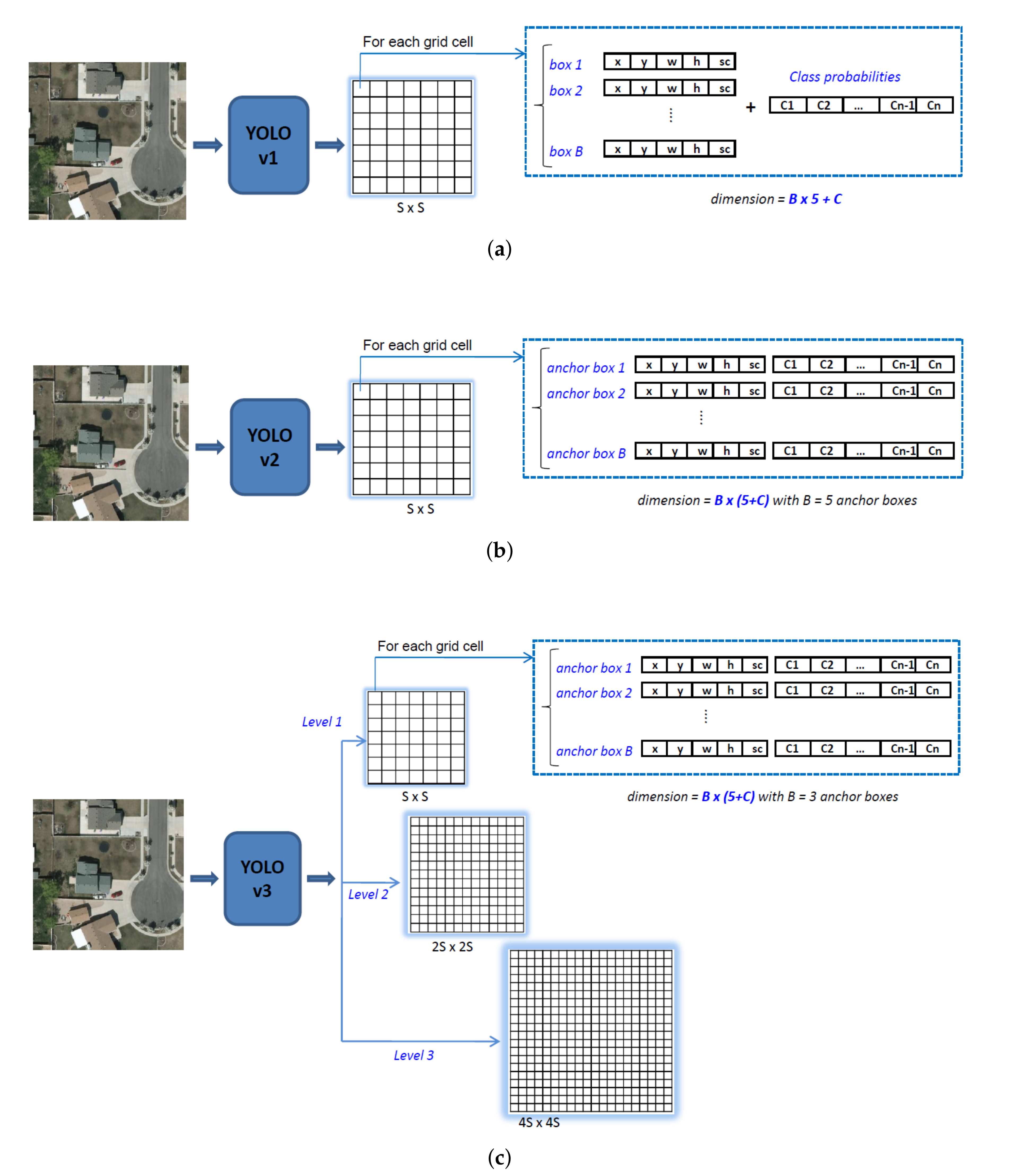
3.1. Inspiration from the YOLO Family
3.2. Proposed Model: YOLO-Fine
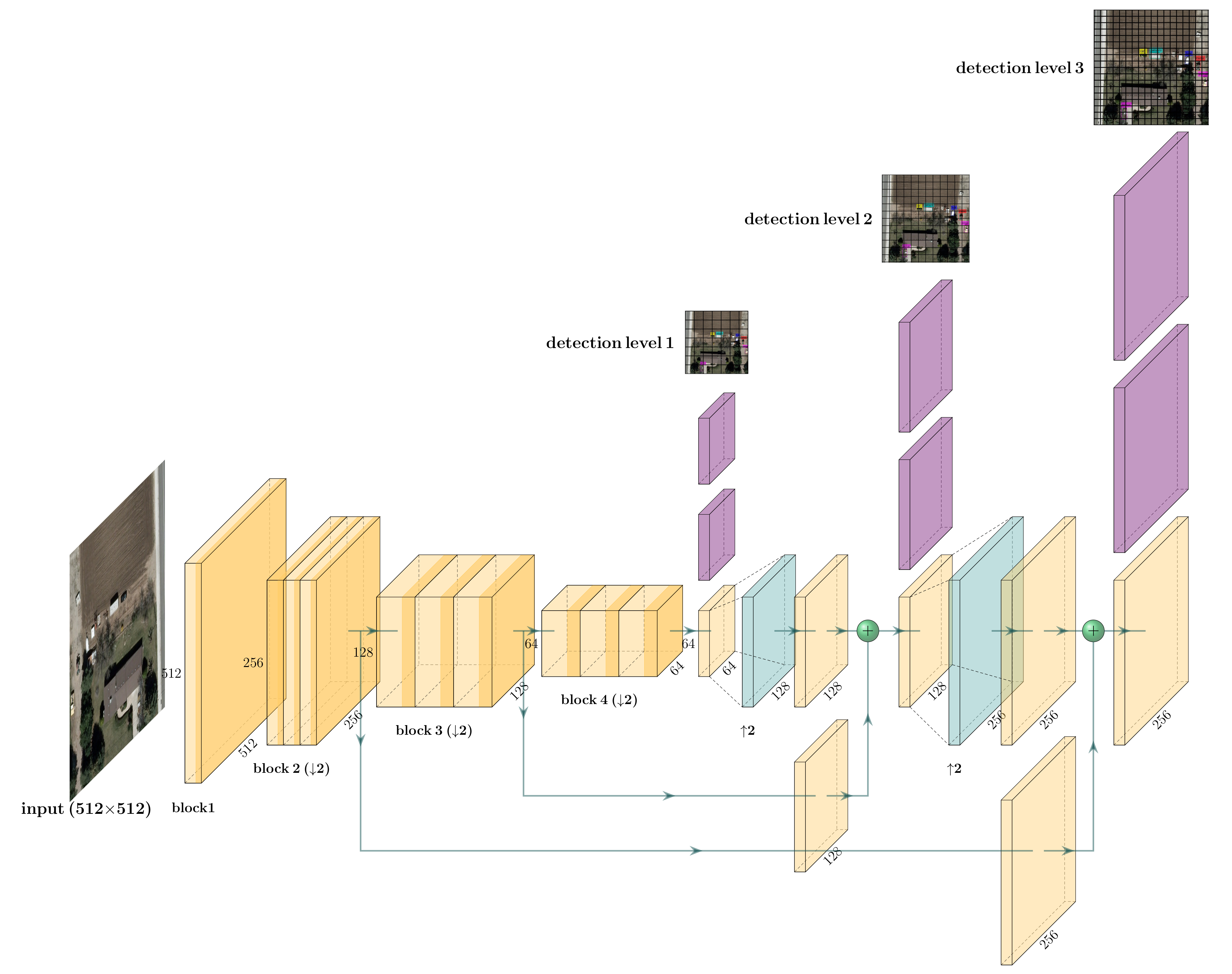
- While YOLOv3 is appealing for operational contexts due to its speed, its performance in detecting small objects remains limited because the input image is divided into three detection grids with subsampling factors of 32, 16, and eight. As a result, YOLOv3 is not able to detect objects measuring less than eight pixels per dimension (height or width) or to discriminate two objects that are closer than eight pixels. The ability of YOLOv3 to detect objects of a wide range of sizes is relevant in numerous computer vision applications, but not in our context of small object detection in remote sensing. The highly sub-sampled layers are then not necessary anymore, thus our first proposition is to remove two coarse detection levels related to large-size objects often observed in natural images. We replace them by two finer detection levels dedicated to lower sub-sampling factors of four and two with skip connections to the corresponding feature maps from high-level layers to those from low-level layers but with very high spatial resolution. The objective is to refine the object search grid in order to be able to recognize and discriminate objects smaller than eight pixels per dimension from the image. Moreover, objects that are relatively close (such as building blocks, cars in a parking, small boats in a harbor, etc.) could be better discriminated.
- In order to facilitate the storage and implementation within an operational context, we also attempt to remove unnecessary convolutional layers from the backbone Darknet-53. Based on our experiments, we found that the last two convolutional blocks of Darknet-53 include a high number of parameters (due to the high number of filters), but are not useful to characterize small objects due to their high subsampling factors. Removing these two blocks results in both a reduction of the number of parameters in YOLO-fine (making it lighter) and of the feature extracting time required by the detector.
- The three-level detection (that does not exist in YOLOv1 and YOLOv2) strongly helps YOLOv3 to search and detect objects at different scales in the same image. However, this comes with a computational burden for both YOLOv3 and our YOLO-fine. Moreover, when refining the search grid, the training and prediction times will also increase from which the compromise between detection accuracy and computing time. The reason that we maintain the three detection levels in YOLO-fine is to make YOLO-fine able to provide good results for various sizes of very small and small objects, as well as provide at least equivalent performance to YOLOv3 on medium or larger objects (i.e., the largest scale of YOLO-fine is the smallest of YOLOv3). To this end, thanks to the efficient behavior of YOLO in general, our YOLO-fine architecture remains able to perform detection in real-time using GPU. We report this accuracy/time trade-off later in the experimental study.
4. Experimental Study
4.1. Datasets
4.1.1. VEDAI
4.1.2. MUNICH
4.1.3. XVIEW
4.2. Experimental Setup and Evaluation Criteria
- Intersection over Union (IoU) is one of the most widely used criteria in the literature to evaluate the object detection task. This criterion measures the overlapping ratio between the detected box and the ground truth box. IoU varies between 0 (no overlap) and 1 (total overlap) and decides if the predicted box is an object or not (according to a threshold to be set). Within our specific case of small object detection, the IoU threshold should be set very low. In our experiments, this threshold was set to for all of the detectors.
- Precision, Recall, F1-score, and mean average precision (mAP) are widely used criteria to evaluate the performance of a model. We remind they are computed, as follows:with TP, FP, and FN denoting True Positive, False Positive, and False Negative, respectively.
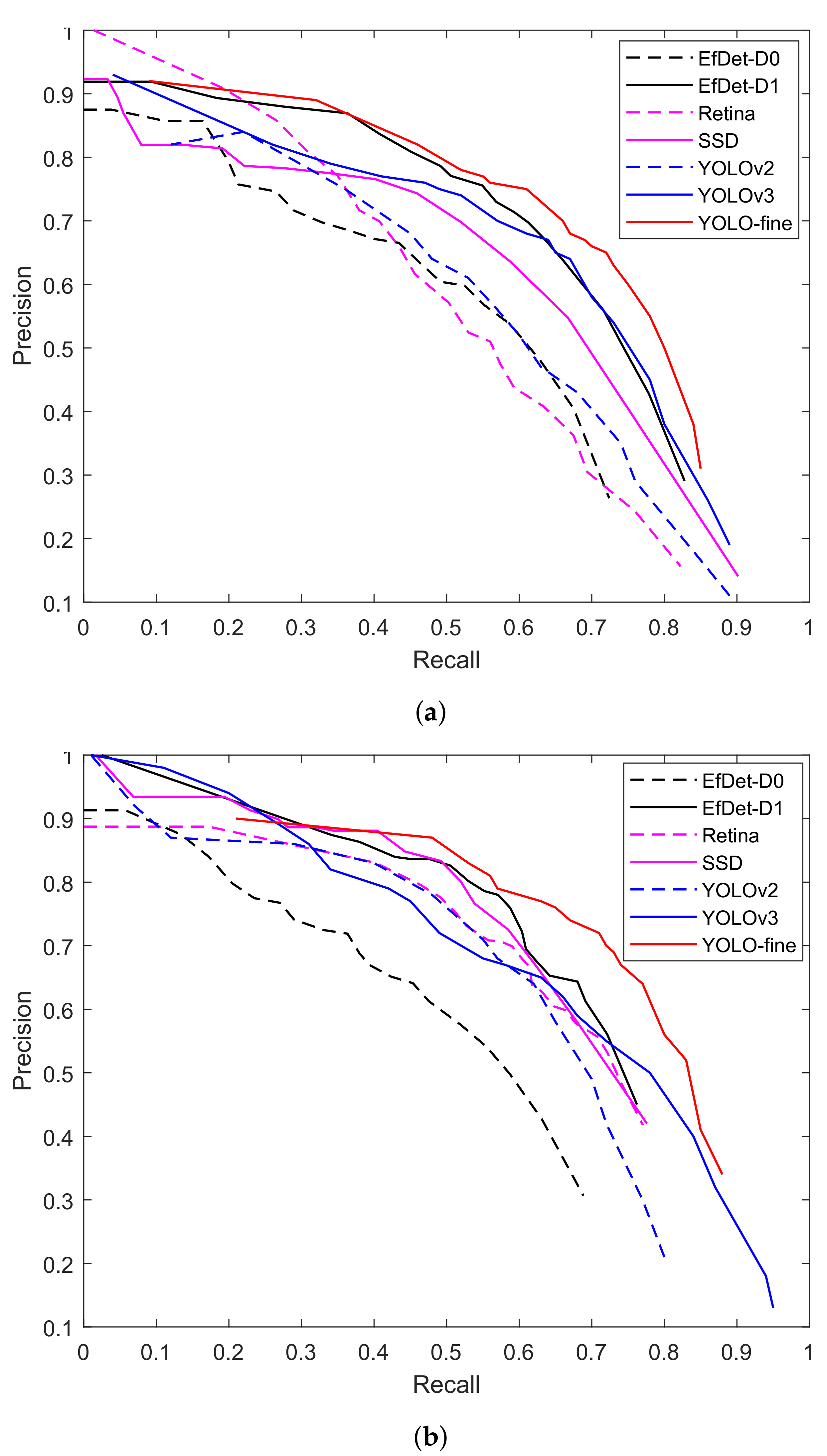
- Precision/Recall curve plots the precision in function of the recall rate. It is a decreasing curve. When we lower the threshold of the detector (the confidence index), the recall increases (as we will detect more objects), but the precision decreases (as our detections are more likely to be false alarms), and vice versa. The visualization of the precision/recall curve gives us a global vision of the compromise between precision and recall.
4.3. Detection Performance
4.3.1. VEDAI512 Color and Infrared
4.3.2. VEDAI1024 Color and Infrared
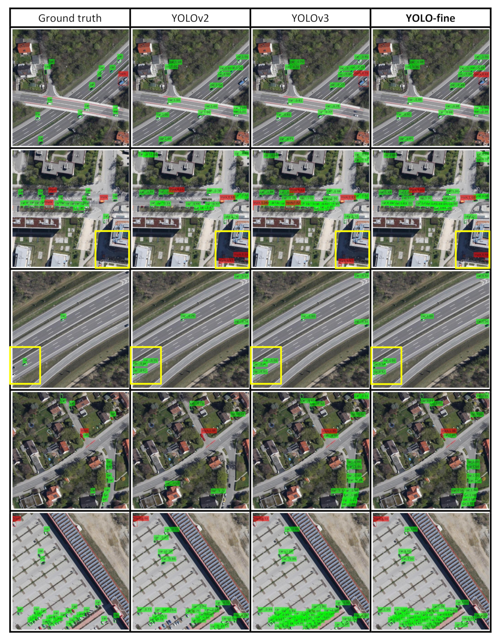
4.3.3. MUNICH
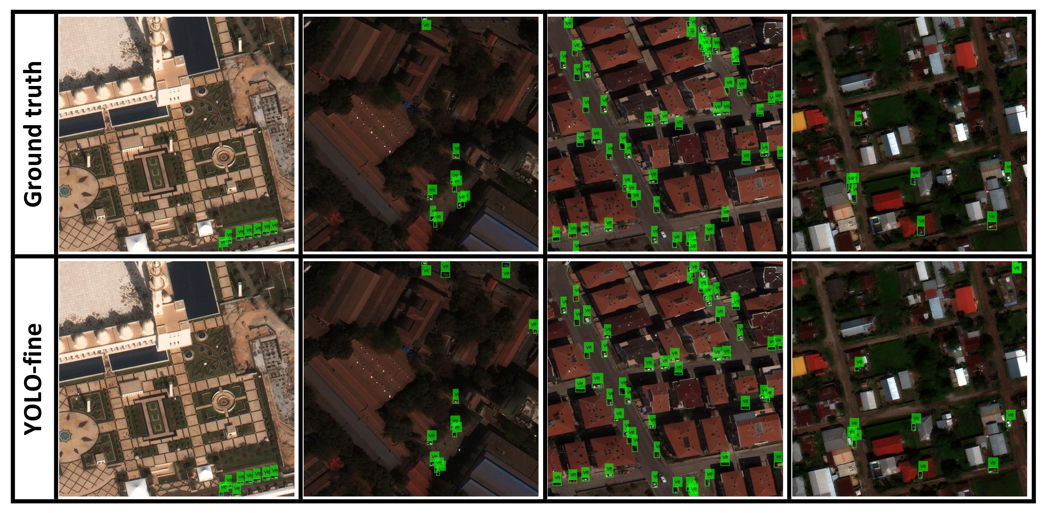
4.3.4. XVIEW
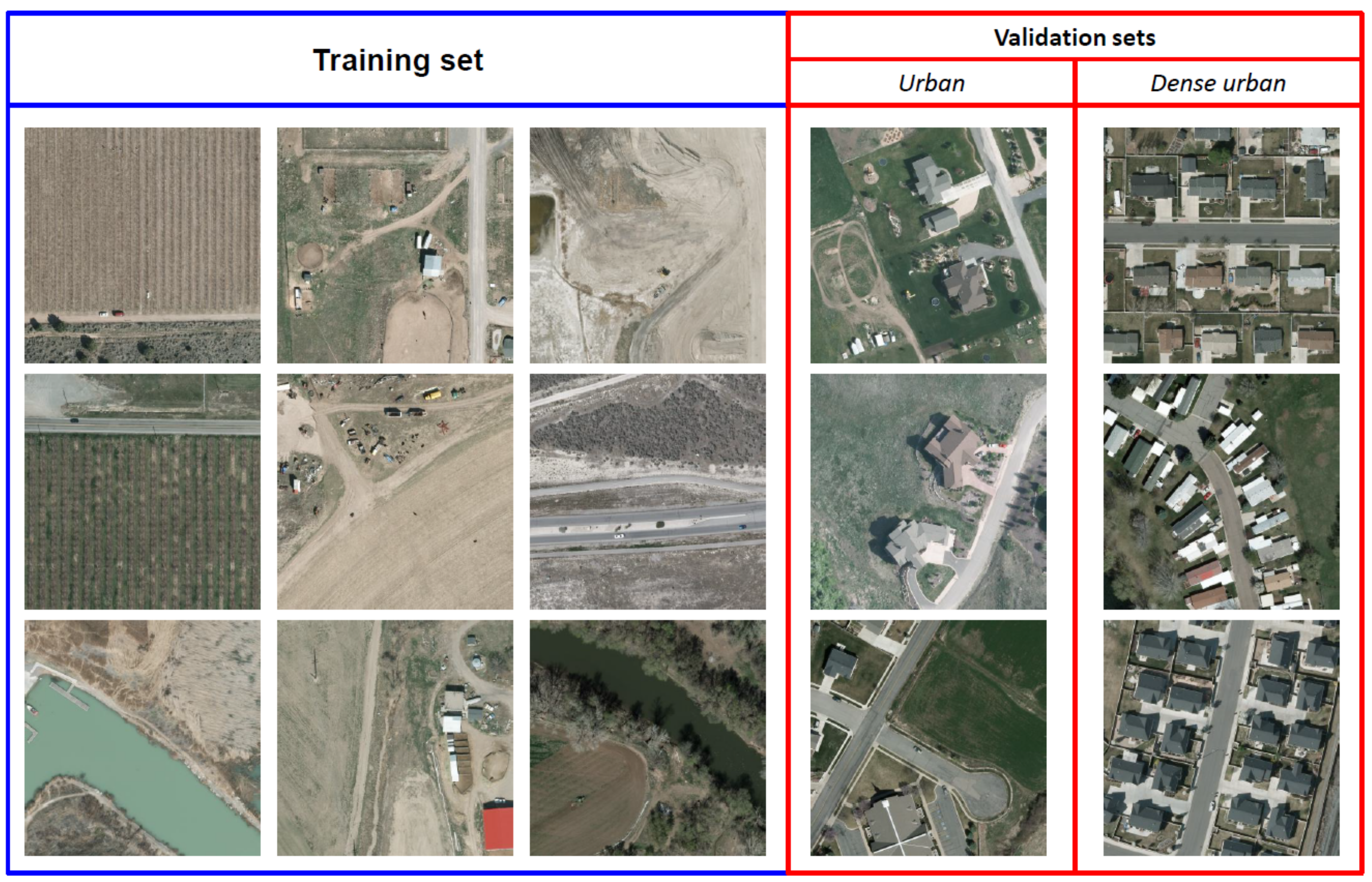
4.4. Effect of New Backgrounds in Validation Sets
4.4.1. Setup
4.4.2. Results
5. Conclusions and Future Works
Author Contributions
Funding
Conflicts of Interest
References
- Zou, Z.; Shi, Z.; Guo, Y.; Ye, J. Object detection in 20 years: A survey. arXiv 2019, arXiv:1905.05055. [Google Scholar]
- Liu, L.; Ouyang, W.; Wang, X.; Fieguth, P.; Chen, J.; Liu, X.; Pietikäinen, M. Deep learning for generic object detection: A survey. Int. J. Comput. Vis. 2020, 128, 261–318. [Google Scholar] [CrossRef]
- Jiao, L.; Zhang, F.; Liu, F.; Yang, S.; Li, L.; Feng, Z.; Qu, R. A survey of deep learning-based object detection. IEEE Access 2019, 7, 128837–128868. [Google Scholar] [CrossRef]
- Girshick, R.; Donahue, J.; Darrell, T.; Malik, J. Rich feature hierarchies for accurate object detection and semantic segmentation. In Proceedings of the IEEE Conference on Computer Vision and Pattern Recognition (CVPR), Columbus, OH, USA, 23–28 June 2014; pp. 580–587. [Google Scholar]
- Girshick, R. Fast R-CNN. In Proceedings of the IEEE International Conference on Computer Vision, Santiago, Chile, 7–13 December 2015; pp. 1440–1448. [Google Scholar]
- Ren, S.; He, K.; Girshick, R.; Sun, J. Faster R-CNN: Towards real-time object detection with region proposal networks. In Proceedings of the Advances in Neural Information Processing Systems (NIPS), Montreal, QC, Canada, 7–12 December 2015; pp. 91–99. [Google Scholar]
- Dai, J.; Li, Y.; He, K.; Sun, J. R-FCN: Object detection via region-based fully convolutional networks. In Proceedings of the Advances in Neural Information Processing Systems (NIPS), Barcelona, Spain, 5–10 December 2016; pp. 379–387. [Google Scholar]
- Lin, T.Y.; Dollár, P.; Girshick, R.; He, K.; Hariharan, B.; Belongie, S. Feature pyramid networks for object detection. In Proceedings of the IEEE Conference on Computer Vision and Pattern Recognition (CVPR), Honolulu, HI, USA, 21–26 July 2017; pp. 2117–2125. [Google Scholar]
- He, K.; Gkioxari, G.; Dollár, P.; Girshick, R. Mask R-CNN. In Proceedings of the IEEE International Conference on Computer Vision (ICCV), Venice, Italy, 22–29 October 2017; pp. 2961–2969. [Google Scholar]
- Redmon, J.; Divvala, S.; Girshick, R.; Farhadi, A. You Only Look Once: Unified, real-time object detection. In Proceedings of the IEEE Conference on Computer Vision and Pattern Recognition (CVPR), Las Vegas, NV, USA, 27–30 June 2016; pp. 779–788. [Google Scholar]
- Redmon, J.; Farhadi, A. YOLO9000: Better, Faster, Stronger. In Proceedings of the IEEE Conference on Computer Vision and Pattern Recognition (CVPR), Honolulu, HI, USA, 21–26 July 2017; pp. 6517–6525. [Google Scholar]
- Redmon, J.; Farhadi, A. Yolov3: An incremental improvement. arXiv 2018, arXiv:1804.02767. [Google Scholar]
- Liu, W.; Anguelov, D.; Erhan, D.; Szegedy, C.; Reed, S.; Fu, C.Y.; Berg, A.C. SSD: Single shot multibox detector. In Proceedings of the European Conference on Computer Vision (ECCV), Amsterdam, The Netherlands, 11–14 October 2016; pp. 21–37. [Google Scholar]
- Shen, Z.; Liu, Z.; Li, J.; Jiang, Y.G.; Chen, Y.; Xue, X. DSOD: Learning deeply supervised object detectors from scratch. In Proceedings of the IEEE International Conference on Computer Vision (ICCV), Venice, Italy, 22–29 October 2017; pp. 1919–1927. [Google Scholar]
- Lin, T.Y.; Goyal, P.; Girshick, R.; He, K.; Dollár, P. Focal loss for dense object detection. In Proceedings of the IEEE International Conference on Computer Vision, Venice, Italy, 22–29 October 2017; pp. 2980–2988. [Google Scholar]
- Kong, T.; Sun, F.; Yao, A.; Liu, H.; Lu, M.; Chen, Y. Ron: Reverse connection with objectness prior networks for object detection. In Proceedings of the IEEE Conference on Computer Vision and Pattern Recognition, Honolulu, HI, USA, 21–26 July 2017; pp. 5936–5944. [Google Scholar]
- Zhao, Q.; Sheng, T.; Wang, Y.; Tang, Z.; Chen, Y.; Cai, L.; Ling, H. M2det: A single-shot object detector based on multi-level feature pyramid network. In Proceedings of the AAAI Conference on Artificial Intelligence, Honolulu, HI, USA, 27 January–1 February 2019; Volume 33, pp. 9259–9266. [Google Scholar]
- Tan, M.; Pang, R.; Le, Q.V. Efficientdet: Scalable and efficient object detection. In Proceedings of the IEEE/CVF Conference on Computer Vision and Pattern Recognition, Seattle, WA, USA, 16–18 June 2020; pp. 10781–10790. [Google Scholar]
- Saito, S.; Aoki, Y. Building and road detection from large aerial imagery. SPIE/IS&T Electron. Imaging 2015, 9405, 94050K. [Google Scholar]
- Cheng, G.; Wang, Y.; Xu, S.; Wang, H.; Xiang, S.; Pan, C. Automatic road detection and centerline extraction via cascaded end-to-end convolutional neural network. IEEE Trans. Geosci. Remote Sens. 2017, 55, 3322–3337. [Google Scholar] [CrossRef]
- Chen, F.; Ren, R.; Van de Voorde, T.; Xu, W.; Zhou, G.; Zhou, Y. Fast automatic airport detection in remote sensing images using convolutional neural networks. Remote Sens. 2018, 10, 443. [Google Scholar] [CrossRef]
- Chen, X.; Xiang, S.; Liu, C.L.; Pan, C.H. Vehicle detection in satellite images by hybrid deep convolutional neural networks. IEEE Geosci. Remote Sens. Lett. 2014, 11, 1797–1801. [Google Scholar] [CrossRef]
- Tang, T.; Zhou, S.; Deng, Z.; Lei, L.; Zou, H. Arbitrary-oriented vehicle detection in aerial imagery with single convolutional neural networks. Remote Sens. 2017, 9, 1170. [Google Scholar] [CrossRef]
- Froidevaux, A.; Julier, A.; Lifschitz, A.; Pham, M.T.; Dambreville, R.; Lefèvre, S.; Lassalle, P. Vehicle detection and counting from VHR satellite images: Efforts and open issues. arXiv 2019, arXiv:1910.10017. [Google Scholar]
- Wu, Y.; Ma, W.; Gong, M.; Bai, Z.; Zhao, W.; Guo, Q.; Chen, X.; Miao, Q. A Coarse-to-Fine Network for Ship Detection in Optical Remote Sensing Images. Remote Sens. 2020, 12, 246. [Google Scholar] [CrossRef]
- Kellenberger, B.; Marcos, D.; Tuia, D. Detecting mammals in UAV images: Best practices to address a substantially imbalanced dataset with deep learning. Remote Sens. Environ. 2018, 216, 139–153. [Google Scholar] [CrossRef]
- Shiu, Y.; Palmer, K.; Roch, M.A.; Fleishman, E.; Liu, X.; Nosal, E.M.; Helble, T.; Cholewiak, D.; Gillespie, D.; Klinck, H. Deep neural networks for automated detection of marine mammal species. Sci. Rep. 2020, 10, 1–12. [Google Scholar] [CrossRef] [PubMed]
- Cheng, G.; Han, J. A survey on object detection in optical remote sensing images. ISPRS J. Photogramm. Remote Sens. 2016, 117, 11–28. [Google Scholar] [CrossRef]
- Zhu, X.X.; Tuia, D.; Mou, L.; Xia, G.S.; Zhang, L.; Xu, F.; Fraundorfer, F. Deep learning in remote sensing: A comprehensive review and list of resources. IEEE Geosci. Remote Sens. Mag. 2017, 5, 8–36. [Google Scholar] [CrossRef]
- Li, K.; Wan, G.; Cheng, G.; Meng, L.; Han, J. Object detection in optical remote sensing images: A survey and a new benchmark. ISPRS J. Photogramm. Remote Sens. 2020, 159, 296–307. [Google Scholar] [CrossRef]
- Razakarivony, S.; Jurie, F. Vehicle detection in aerial imagery: A small target detection benchmark. J. Vis. Commun. Image Represent. 2016, 34, 187–203. [Google Scholar] [CrossRef]
- Liu, K.; Mattyus, G. DLR 3k Munich Vehicle Aerial Image Dataset. 2015. Available online: https://pba-freesoftware.eoc.dlr.de/MunichDatasetVehicleDetection-2015-old.zip (accessed on 4 August 2020).
- Lam, D.; Kuzma, R.; McGee, K.; Dooley, S.; Laielli, M.; Klaric, M.; Bulatov, Y.; McCord, B. XView: Objects in context in overhead imagery. arXiv 2018, arXiv:1802.07856. [Google Scholar]
- Tong, K.; Wu, Y.; Zhou, F. Recent advances in small object detection based on deep learning: A review. Image Vis. Comput. 2020, 103910. [Google Scholar] [CrossRef]
- Eggert, C.; Brehm, S.; Winschel, A.; Zecha, D.; Lienhart, R. A closer look: Small object detection in faster R-CNN. In Proceedings of the 2017 IEEE International Conference on Multimedia and Expo (ICME), Hong Kong, China, 10–14 July 2017; IEEE: Piscataway, NJ, USA, 2017; pp. 421–426. [Google Scholar]
- Cao, C.; Wang, B.; Zhang, W.; Zeng, X.; Yan, X.; Feng, Z.; Liu, Y.; Wu, Z. An improved faster R-CNN for small object detection. IEEE Access 2019, 7, 106838–106846. [Google Scholar] [CrossRef]
- Cao, G.; Xie, X.; Yang, W.; Liao, Q.; Shi, G.; Wu, J. Feature-fused SSD: Fast detection for small objects. In Proceedings of the Ninth International Conference on Graphic and Image Processing (ICGIP 2017), Qingdao, China, 14–16 October 2017; International Society for Optics and Photonics: Bellingham, WA, USA, 2018; Volume 10615, p. 106151E. [Google Scholar]
- Cui, L.; Ma, R.; Lv, P.; Jiang, X.; Gao, Z.; Zhou, B.; Xu, M. Mdssd: Multi-scale deconvolutional single shot detector for small objects. arXiv 2018, arXiv:1805.07009. [Google Scholar] [CrossRef]
- Zhang, S.; Wen, L.; Bian, X.; Lei, Z.; Li, S.Z. Single-shot refinement neural network for object detection. In Proceedings of the IEEE Conference on Computer Vision and Pattern Recognition, Salt Lake City, UT, USA, 18–22 June 2018; pp. 4203–4212. [Google Scholar]
- Guan, L.; Wu, Y.; Zhao, J. Scan: Semantic context aware network for accurate small object detection. Int. J. Comput. Intell. Syst. 2018, 11, 951–961. [Google Scholar] [CrossRef]
- Ren, Y.; Zhu, C.; Xiao, S. Small object detection in optical remote sensing images via modified faster R-CNN. Appl. Sci. 2018, 8, 813. [Google Scholar] [CrossRef]
- Ding, P.; Zhang, Y.; Deng, W.J.; Jia, P.; Kuijper, A. A light and faster regional convolutional neural network for object detection in optical remote sensing images. ISPRS J. Photogramm. Remote Sens. 2018, 141, 208–218. [Google Scholar] [CrossRef]
- Zhang, S.; He, G.; Chen, H.B.; Jing, N.; Wang, Q. Scale adaptive proposal network for object detection in remote sensing images. IEEE Geosci. Remote Sens. Lett. 2019, 16, 864–868. [Google Scholar] [CrossRef]
- Zhang, W.; Wang, S.; Thachan, S.; Chen, J.; Qian, Y. Deconv R-CNN for small object detection on remote sensing images. In Proceedings of the IEEE International Geoscience and Remote Sensing Symposium (IGARSS), Valencia, Spain, 22–27 July 2018; pp. 2483–2486. [Google Scholar]
- Ren, Y.; Zhu, C.; Xiao, S. Deformable Faster R-CNN with aggregating multi-layer features for partially occluded object detection in optical remote sensing images. Remote Sens. 2018, 10, 1470. [Google Scholar] [CrossRef]
- Yan, J.; Wang, H.; Yan, M.; Diao, W.; Sun, X.; Li, H. IoU-adaptive deformable R-CNN: Make full use of IoU for multi-class object detection in remote sensing imagery. Remote Sens. 2019, 11, 286. [Google Scholar] [CrossRef]
- Xia, G.S.; Bai, X.; Ding, J.; Zhu, Z.; Belongie, S.; Luo, J.; Datcu, M.; Pelillo, M.; Zhang, L. DOTA: A large-scale dataset for object detection in aerial images. In Proceedings of the IEEE Conference on Computer Vision and Pattern Recognition (CVPR), Salt Lake City, UT, USA, 18–22 June 2018; pp. 3974–3983. [Google Scholar]
- Liu, J.; Yang, S.; Tian, L.; Guo, W.; Zhou, B.; Jia, J.; Ling, H. Multi-component fusion network for small object detection in remote sensing images. IEEE Access 2019, 7, 128339–128352. [Google Scholar] [CrossRef]
- Pang, J.; Li, C.; Shi, J.; Xu, Z.; Feng, H. R2CNN: Fast tiny object detection in large-scale remote sensing images. IEEE Trans. Geosci. Remote Sens. 2019, 57, 5512–5524. [Google Scholar] [CrossRef]
- Yang, X.; Yang, J.; Yan, J.; Zhang, Y.; Zhang, T.; Guo, Z.; Sun, X.; Fu, K. SCRDet: Towards more robust detection for small, cluttered and rotated objects. In Proceedings of the IEEE International Conference on Computer Vision (ICCV), Seoul, Korea, 3 November–27 October 2019; pp. 8232–8241. [Google Scholar]
- Liu, M.; Wang, X.; Zhou, A.; Fu, X.; Ma, Y.; Piao, C. UAV-YOLO: Small Object Detection on Unmanned Aerial Vehicle Perspective. Sensors 2020, 20, 2238. [Google Scholar] [CrossRef]
- Zhao, K.; Ren, X. Small aircraft detection in remote sensing images based on YOLOv3. In Proceedings of the International Conference on Electrical Engineering, Control and Robotics (EECR), Guangzhou, China, 12–14 January 2019; Volume 533. [Google Scholar]
- Nina, W.; Condori, W.; Machaca, V.; Villegas, J.; Castro, E. Small ship detection on optical satellite imagery with YOLO and YOLT. In Proceedings of the Future of Information and Communication Conference (FICC), San Francisco, CA, USA, 5–6 March 2020; pp. 664–677. [Google Scholar]
- Xie, Y.; Cai, J.; Bhojwani, R.; Shekhar, S.; Knight, J. A locally-constrained YOLO framework for detecting small and densely-distributed building footprints. Int. J. Geogr. Inf. Sci. 2020, 34, 777–801. [Google Scholar] [CrossRef]
- Van Etten, A. You Only Look Twice: Rapid multi-scale object detection in satellite imagery. arXiv 2018, arXiv:1805.09512. [Google Scholar]
- Huang, Z.; Wang, J.; Fu, X.; Yu, T.; Guo, Y.; Wang, R. DC-SPP-YOLO: Dense connection and spatial pyramid pooling based YOLO for object detection. Inf. Sci. 2020, 522, 241–258. [Google Scholar] [CrossRef]
- Li, C. High Quality, Fast, Modular Reference Implementation of SSD in PyTorch. 2018. Available online: https://github.com/lufficc/SSD (accessed on 4 August 2020).
- Massa, F.; Girshick, R. Maskrcnn-Benchmark: Fast, Modular Reference Implementation of Instance Segmentation and Object Detection Algorithms in PyTorch. 2018. Available online: https://github.com/facebookresearch/maskrcnn-benchmark (accessed on 4 August 2020).


| Parameters | Models | |||
|---|---|---|---|---|
| YOLO [10] | YOLOv2 [11] | YOLOv3 [12] | YOLO-Fine (Ours) | |
| Number of layers | 31 | 31 | 106 | 68 |
| Multilevel prediction | - | - | 3 levels | 3 levels |
| Anchor boxes | - | 5 | 3 | 3 |
| 416 × 416 | 320 × 320 | |||
| Input image size | 448 × 448 | 544 × 544 | 416 × 416 | 512 × 512 |
| 608 × 608 | 608 × 608 | |||
| Size of weight file | 753 MB | 258 MB | 237 MB | 18 MB |
| Parameters | Datasets | |||
|---|---|---|---|---|
| VEDAI1024 | VEDAI512 | MUNICH | XVIEW | |
| Number of images | 1200 | 1200 | 1566 | 7.4 k |
| in the train set | 1089 | 1089 | 1226 | 5.5 k |
| in the validation set | 121 | 121 | 340 | 1.9 k |
| Number of classes | 8 | 8 | 2 | 1 |
| Number of objects | 3757 | 3757 | 9460 | 35 k |
| Spatial resolution | 12.5 cm | 25 cm | 26 cm | 30 cm |
| Object size (pixels) | 16 → 40 | 8 → 20 | 8 → 20 | 6 → 15 |
| (a) Classwise accuracy and mean average precision. Best results in bold. | |||||||||
| Model | Car | Truck | Pickup | Tractor | Camping | Boat | Van | Other | mAP |
| SSD | 73.92 | 49.70 | 67.31 | 52.03 | 57.00 | 41.52 | 53.36 | 39.99 | 54.35 |
| EfficientDet(D0) | 64.45 | 38.63 | 51.57 | 27.91 | 57.14 | 17.19 | 15.34 | 27.81 | 37.50 |
| EfficientDet(D1) | 69.08 | 61.20 | 65.74 | 47.18 | 69.08 | 33.65 | 16.55 | 36.67 | 51.36 |
| Faster R-CNN | 72.91 | 48.98 | 66.38 | 55.61 | 61.61 | 30.29 | 35.95 | 35.34 | 50.88 |
| RetinaNet(50) | 60.61 | 35.98 | 63.82 | 19.36 | 65.16 | 21.55 | 46.60 | 09.51 | 40.33 |
| YOLOv2 | 72.65 | 50.24 | 62.83 | 67.46 | 56.53 | 42.33 | 60.95 | 56.73 | 58.72 |
| YOLOv3 | 75.22 | 73.53 | 65.69 | 57.02 | 59.27 | 47.20 | 71.55 | 47.20 | 62.09 |
| YOLOv3-tiny | 64.11 | 41.21 | 48.38 | 30.04 | 42.37 | 24.64 | 68.25 | 40.77 | 44.97 |
| YOLOv3-spp | 79.03 | 68.57 | 72.30 | 61.67 | 63.41 | 44.26 | 60.68 | 42.43 | 61.57 |
| YOLO-fine | 76.77 | 63.45 | 74.35 | 78.12 | 64.74 | 70.04 | 77.91 | 45.04 | 68.18 |
| (b) Overall evaluation metrics. Best result of F1-score in bold. | |||||||||
| Model | TP | FP | FN | Precision | Recall | F1-Score | |||
| SSD | 188 | 81 | 178 | 0.69 | 0.51 | 0.59 | |||
| EfficientDet(D0) | 198 | 143 | 168 | 0.58 | 0.54 | 0.56 | |||
| EfficientDet(D1) | 250 | 164 | 116 | 0.60 | 0.68 | 0.64 | |||
| Faster R-CNN | 260 | 277 | 106 | 0.48 | 0.71 | 0.57 | |||
| RetinaNet(50) | 216 | 236 | 150 | 0.47 | 0.59 | 0.52 | |||
| YOLOv2 | 209 | 162 | 157 | 0.56 | 0.57 | 0.57 | |||
| YOLOv3 | 246 | 139 | 120 | 0.64 | 0.67 | 0.66 | |||
| YOLOv3-tiny | 163 | 151 | 203 | 0.52 | 0.45 | 0.48 | |||
| YOLOv3-spp | 244 | 103 | 122 | 0.69 | 0.67 | 0.68 | |||
| YOLO-fine | 258 | 133 | 108 | 0.67 | 0.70 | 0.69 | |||
| (a) Classwise accuracy and mean average precision. Best results in bold. | |||||||||
| Model | Car | Truck | Pickup | Tractor | Camping | Boat | Van | Other | mAP |
| SSD | 78.72 | 51.27 | 65.50 | 55.98 | 59.25 | 42.99 | 61.21 | 36.68 | 56.45 |
| EfficientDet(D0) | 64.48 | 44.08 | 51.57 | 27.72 | 53.32 | 18.88 | 4.94 | 24.59 | 36.20 |
| EfficientDet(D1) | 78.72 | 51.43 | 63.86 | 43.11 | 68.79 | 17.80 | 42.99 | 27.92 | 49.33 |
| Faster R-CNN | 75.24 | 48.87 | 62.95 | 35.55 | 60.14 | 31.07 | 39.20 | 13.11 | 45.77 |
| RetinaNet(50) | 73.58 | 44.50 | 65.98 | 21.65 | 64.37 | 32.93 | 28.04 | 22.20 | 44.16 |
| YOLOv2 | 73.47 | 57.18 | 68.67 | 46.25 | 63.70 | 34.71 | 36.55 | 22.35 | 50.36 |
| YOLOv3 | 85.58 | 56.46 | 79.12 | 54.77 | 55.79 | 55.02 | 75.96 | 38.49 | 62.65 |
| YOLOv3-tiny | 66.63 | 34.36 | 56.28 | 37.42 | 43.70 | 31.59 | 75.52 | 31.30 | 46.72 |
| YOLOv3-spp | 84.23 | 71.54 | 73.12 | 55.92 | 65.08 | 50.07 | 70.00 | 38.52 | 63.56 |
| YOLO-fine | 79.68 | 80.97 | 74.49 | 70.65 | 77.09 | 60.84 | 63.56 | 37.33 | 68.83 |
| (b) Overall evaluation metrics. Best result of F1-score in bold. | |||||||||
| Model | TP | FP | FN | Precision | Recall | F1-Score | |||
| SSD | 196 | 59 | 170 | 0.76 | 0.53 | 0.63 | |||
| EfficientDet(D0) | 188 | 139 | 178 | 0.57 | 0.51 | 0.54 | |||
| EfficientDet(D1) | 233 | 125 | 133 | 0.65 | 0.63 | 0.64 | |||
| Faster R-CNN | 247 | 314 | 119 | 0.44 | 0.67 | 0.53 | |||
| RetinaNet(50) | 248 | 180 | 118 | 0.58 | 0.67 | 0.62 | |||
| YOLOv2 | 203 | 84 | 163 | 0.71 | 0.55 | 0.62 | |||
| YOLOv3 | 241 | 146 | 125 | 0.62 | 0.66 | 0.64 | |||
| YOLOv3-tiny | 176 | 181 | 190 | 0.49 | 0.48 | 0.49 | |||
| YOLOv3-spp | 239 | 129 | 127 | 0.65 | 0.65 | 0.65 | |||
| YOLO-fine | 262 | 112 | 104 | 0.70 | 0.72 | 0.71 | |||
| Color Version | Infrared Version | |||||||
|---|---|---|---|---|---|---|---|---|
| Model | Precision | Recall | F1-Score | mAP | Precision | Recall | F1-Score | mAP |
| SSD | 0.76 | 0.69 | 0.72 | 70.91 | 0.76 | 0.70 | 0.73 | 69.83 |
| EfficientDet(D0) | 0.75 | 0.89 | 0.77 | 70.68 | 0.77 | 0.75 | 0.76 | 69.79 |
| EfficientDet(D1) | 0.79 | 0.80 | 0.79 | 74.01 | 0.78 | 0.78 | 0.78 | 71.23 |
| Faster R-CNN | 0.64 | 0.81 | 0.71 | 70.22 | 0.47 | 0.69 | 0.56 | 56.41 |
| RetinaNet(50) | 0.59 | 0.75 | 0.66 | 61.47 | 0.60 | 0.80 | 0.69 | 67.59 |
| YOLOv2 | 0.66 | 0.73 | 0.69 | 65.72 | 0.68 | 0.67 | 0.68 | 63.16 |
| YOLOv3 | 0.74 | 0.79 | 0.76 | 73.11 | 0.8 | 0.72 | 0.76 | 71.01 |
| YOLOv3-tiny | 0.65 | 0.58 | 0.61 | 55.55 | 0.66 | 0.58 | 0.62 | 55.36 |
| YOLOv3-spp | 0.79 | 0.76 | 0.77 | 75.04 | 0.78 | 0.74 | 0.76 | 73.70 |
| YOLO-fine | 0.79 | 0.77 | 0.78 | 76.00 | 0.80 | 0.74 | 0.76 | 75.17 |
| Model | Car | Truck | mAP | Precision | Recall | F1-Score |
|---|---|---|---|---|---|---|
| SSD | 99.31 | 95.83 | 97.57 | 0.98 | 0.97 | 0.98 |
| EfficientDet(D0) | 92.72 | 89.09 | 90.90 | 0.98 | 0.82 | 0.90 |
| EfficientDet(D1) | 97.65 | 94.78 | 96.22 | 0.98 | 0.82 | 0.90 |
| Faster-RCNN | 90.96 | 94.92 | 92.94 | 0.96 | 0.92 | 0.94 |
| RetinaNet(50) | 80.89 | 78.81 | 79.85 | 0.76 | 0.74 | 0.75 |
| YOLOv2 | 70.23 | 89.28 | 79.76 | 0.90 | 0.59 | 0.71 |
| YOLOv3 | 99.15 | 96.59 | 97.87 | 0.84 | 0.99 | 0.91 |
| YOLOv3-tiny | 92.28 | 93.57 | 92.92 | 0.81 | 0.92 | 0.86 |
| YOLOv3-spp | 96.39 | 94.77 | 95.58 | 0.90 | 0.88 | 0.89 |
| YOLO-fine | 99.93 | 99.45 | 99.69 | 0.96 | 1.00 | 0.98 |
| Model | Precision | Recall | F1-Score | mAP |
|---|---|---|---|---|
| SSD | 0.80 | 0.62 | 0.70 | 68.09 |
| EfficientDet(D0) | 0.84 | 0.78 | 0.81 | 82.45 |
| EfficientDet(D1) | 0.80 | 0.75 | 0.78 | 82.51 |
| Faster R-CNN | 0.50 | 0.72 | 0.59 | 57.01 |
| RetinaNet(50) | 0.70 | 0.21 | 0.33 | 34.84 |
| YOLOv2 | 0.75 | 0.41 | 0.53 | 47.68 |
| YOLOv3 | 0.77 | 0.74 | 0.75 | 78.93 |
| YOLOv3-tiny | 0.66 | 0.61 | 0.64 | 62.03 |
| YOLOv3-spp | 0.81 | 0.73 | 0.77 | 77.34 |
| YOLO-fine | 0.87 | 0.72 | 0.79 | 84.34 |
| Weight Size | Prediction Time/Image (ms) | Number of Frames/Second (FPS) | ||||||
|---|---|---|---|---|---|---|---|---|
| Model | (MB) | BFLOPS | Titan X | RTX 2080ti | V100 | Titan X | RTX 2080ti | V100 |
| YOLOv2 | 202.4 | 44.44 | 17.6 | 11.9 | 10.4 | 57 | 84 | 97 |
| YOLOv3 | 246.3 | 98.92 | 26.9 | 14.5 | 11.4 | 37 | 69 | 88 |
| YOLOv3-tiny | 34.7 | 8.25 | 5.7 | 5.2 | 4.6 | 176 | 193 | 215 |
| YOLOv3-spp | 250.5 | 99.50 | 28.5 | 15.5 | 11.9 | 35 | 64 | 84 |
| YOLO-fine | 18.5 | 63.16 | 29.5 | 18.1 | 11.9 | 34 | 55 | 84 |
| Parameters | Set | ||
|---|---|---|---|
| Train Set | Validation Set 1 | Validation Set 2 | |
| Environment | rural, forest, desert | urban | dense urban |
| Number of images | 870 | 232 | 143 |
| Number of objects | 2142 | 815 | 797 |
| from class Car | 716 | 279 | 381 |
| from class Truck | 248 | 42 | 17 |
| from class Pickup | 505 | 235 | 215 |
| from class Tractor | 147 | 40 | 3 |
| from class Camping | 151 | 132 | 113 |
| from class Ship | 87 | 38 | 45 |
| from class Van | 63 | 25 | 13 |
| from class Other | 208 | 24 | 10 |
| Perfomance | Background 1 | Background 2 | ||||
|---|---|---|---|---|---|---|
| YOLOv2 | YOLOv3 | YOLO-Fine | YOLOv2 | YOLOv3 | YOLO-Fine | |
| car | 52.48 | 70.42 | 75.23 | 61.58 | 77.55 | 81.32 |
| truck | 27.71 | 56.53 | 68.08 | 46.49 | 55.86 | 61.29 |
| pickup | 49.63 | 63.74 | 73.78 | 32.77 | 53.02 | 60.93 |
| tractor | 52.23 | 47.81 | 68.52 | 38.67 | 44.44 | 41.67 |
| camping | 46.62 | 56.81 | 62.84 | 43.49 | 51.58 | 62.40 |
| boat | 38.76 | 55.13 | 63.07 | 0.93 | 21.56 | 22.28 |
| van | 19.58 | 62.26 | 59.85 | 8.39 | 42.44 | 53.18 |
| other | 15.24 | 32.17 | 30.79 | 15.29 | 2.50 | 6.61 |
| mAP | 37.78 | 55.68 | 62.79 | 30.95 | 43.37 | 48.71 |
| Precision | 0.59 | 0.66 | 0.67 | 0.60 | 0.69 | 0.63 |
| Recall | 0.41 | 0.54 | 0.68 | 0.40 | 0.54 | 0.65 |
| F1-score | 0.48 | 0.60 | 0.67 | 0.48 | 0.60 | 0.64 |
© 2020 by the authors. Licensee MDPI, Basel, Switzerland. This article is an open access article distributed under the terms and conditions of the Creative Commons Attribution (CC BY) license (http://creativecommons.org/licenses/by/4.0/).
Share and Cite
Pham, M.-T.; Courtrai, L.; Friguet, C.; Lefèvre, S.; Baussard, A. YOLO-Fine: One-Stage Detector of Small Objects Under Various Backgrounds in Remote Sensing Images. Remote Sens. 2020, 12, 2501. https://doi.org/10.3390/rs12152501
Pham M-T, Courtrai L, Friguet C, Lefèvre S, Baussard A. YOLO-Fine: One-Stage Detector of Small Objects Under Various Backgrounds in Remote Sensing Images. Remote Sensing. 2020; 12(15):2501. https://doi.org/10.3390/rs12152501
Chicago/Turabian StylePham, Minh-Tan, Luc Courtrai, Chloé Friguet, Sébastien Lefèvre, and Alexandre Baussard. 2020. "YOLO-Fine: One-Stage Detector of Small Objects Under Various Backgrounds in Remote Sensing Images" Remote Sensing 12, no. 15: 2501. https://doi.org/10.3390/rs12152501
APA StylePham, M.-T., Courtrai, L., Friguet, C., Lefèvre, S., & Baussard, A. (2020). YOLO-Fine: One-Stage Detector of Small Objects Under Various Backgrounds in Remote Sensing Images. Remote Sensing, 12(15), 2501. https://doi.org/10.3390/rs12152501