Abstract
In surface mining, rockfall can seriously threaten the safety of personnel located at the base of highwalls and cause serious damage to equipment and machinery. Close-range photogrammetry for the continuous monitoring of rock surfaces represents a valid tool to efficiently assess the potential rockfall hazard and estimate the risk in the affected areas. This work presents an autonomous terrestrial stereo-pair photogrammetric monitoring system developed to observe volumes falling from sub-vertical rock faces located in surface mining environments. The system has the versatility for rapid installation and quick relocation in areas often constrained by accessibility and safety issues and it has the robustness to tolerate the rough environmental conditions typical of mining operations. It allows the collection of synchronised images at different periods with high-sensitivity digital single-lens reflex cameras, producing accurate digital surface models (DSM) of the rock face. Comparisons between successive DSMs can detect detachments and surface movements during defined observation periods. Detailed analysis of the changes in the rock surface, volumes and frequency of the rocks dislodging from the sub-vertical rock surfaces can provide accurate information on event magnitude and return period at very reasonable cost and, therefore, can generate the necessary data for a detailed inventory of the rockfall spatial-temporal occurrence and magnitude. The system was first validated in a trial site, and then applied on a mine site located in NSW (Australia). Results were analysed in terms of multi-temporal data acquired over a period of seven weeks. The excellent detail of the data allowed trends in rockfall event to be correlated to lithology and rainfall events, demonstrating the capability of the system to generate useful data that would otherwise require extended periods of direct observation.
1. Introduction
Rock mass instabilities involving the detachment of rocks of various sizes from vertical or sub-vertical rock faces created during resource exploitation activities represent a significant safety hazard for personnel and machinery located at the base of rock walls [1]. Robust monitoring and thorough geostructural characterization of the rock walls are most important for the early identification of the potential hazards and for an efficient risk assessment and management approach. This is particularly relevant to manage safety and ensure the continuity of the production in areas where highwalls are subjected to rapid changes over time (sometime only 3 to 4 weeks) in response to the mining activity.
Over the last few decades, qualitative and quantitative hazard methodologies have been proposed to assess the hazards associated with rockfall phenomena along transportation corridors, below mountain slopes and on mines sites [2]. While qualitative methods rely on the qualitative ranking of attributes (or classes) of the rock surface and apply well for extended surfaces, quantitative approaches require a significant amount of data to conduct site-specific rockfall energy (intensity)–frequency analyses. Qualitative site-specific observations, or historical data, and trajectory simulations generally infer frequency–magnitude curves. Precursory rockfall events (when observed) and correlations of rockfall occurrence with weather conditions, have also been recognised to provide valid support to hazard and risk assessments and to extrapolate subsequent instability rates [3,4]. While observations on the role of weather, and in particular rainfall events, in rockfall potential detachment, date back to the early 1960s [5,6,7], the quantification of this relationship has been addressed in more recent research [8,9,10]. Most of these studies recognise quite a variability (randomness) in the accumulation of rockfalls in correspondence to a rapid increase in cumulative rainfall, both in short and long term (several years) databases. Therefore, probabilistic models have been proposed to predict rockfall temporal variability according to different weather triggers [8,11,12]. One of the main open issues remains the ability to gather real-time topographic and structural data of the potentially affected areas to support the correlations and reduce the uncertainties.
Spatial data models are nowadays commonly employed to extract the rock mass geo-structural feature data, to monitor rock slopes activities and to predict their evolution [13,14]. Several surveying and monitoring techniques have been proposed over the last few decades to improve prediction capabilities and design appropriate mitigation measures in the areas potentially affected. In particular, proximity remote sensing techniques have been adopted into well-established monitoring systems for rock mechanics applications. However, the choice of the most suitable technique is based on site-specific environmental conditions, accessibility and dimensions of the monitored surface (e.g., object), expected accuracy and spatial/temporal resolution of the data, and finally, but not least, available budgets [15].
Traditional topographical methods obtain frequency and intensity data by measuring the coordinates of selected target locations at different periods and the difference in their positions between consecutive models. These methods have the advantage of being very accurate (0.2–2.0 cm) with potential for automation [16,17]. However, an inherent drawback is the sparseness of measurements, that provides only pointwise (a priori defined) observations. This represents a significant issue for the identification of unanticipated rock slope instabilities, such as rockfalls, for which more detailed digital surface models (DSM) are required [18].
Alternatively, detailed three-dimensional (3D) models of rock slopes [19] can be successfully obtained by satellite, airborne and ground-based (GB) platforms such as Synthetic Aperture Radar Interferometry (InSAR), Light Detection and Ranging (LiDAR) and photogrammetry [18]. These systems allow for high-resolution data acquisition, device portability and easy and fast data processing. Additionally, systematic data acquisition can enhance the implementation of effective early warning systems for slope instability [20,21,22,23]. GB InSAR systems and terrestrial LiDAR (also known as terrestrial laser scanning, TLS) have been successfully applied for rockfall monitoring in civil and mining applications over the last two decades [13,14,24,25,26,27,28,29,30,31,32,33]. Recently, Kromer et al. [34,35] proposed applying TLS acquisition combined with change detection processing workflows for rockfall assessment and forecasting. Periodic measurements were used to build a database of failure events including location, volume and kinematics of potential rockfalls. Similarly, Williams et al. [36] captured rockfall magnitude–frequency data from a single viewpoint TLS, highlighting the influence of temporal acquisition rate on the magnitude of the events and on the uncertainty of volumetric calculation. The results are quite accurate (from few mm to 1 cm), allowing the monitoring of specific sections of a rock face with high spatial resolution remotely and continuously in near-real time, regardless of the atmospheric conditions. However, complexity and costs associated to such systems often represent a limitation to their application.
Photogrammetry, which features simplicity of components and high scalability, represents a valid cost-effective alternative solution. It has been long used to periodically monitor the evolution of landslides or evolving slope instabilities, from aerial images [37] and from the ground [38]. The dislodgment of rocks from a rock surface can be efficiently obtained by comparison of 3D models built at different periods. Additionally, recent Structure from Motion (SfM) and Multi-View Stereo (MVS) processing ‘pipelines’ have significantly marked the automatic generation of accurate and high spatial resolution dense point clouds enabling real or near-real time 3D measurements [39]. The use of photogrammetry in various surface mining applications has nowadays become a mainstream practice [40,41,42,43]. More recently, on-site permanent installations of cameras for monitoring purposes have received increased attention in the scientific literature [44,45,46,47,48,49,50,51,52].
In 2014, Roncella et al. [46] presented a high-resolution, fixed-base, stereo-photogrammetry monitoring system to record the displacement of a landslides located in the European Alps. In the current study, the system proposed by Roncella et al. [46] is further developed and customised to account for rough environmental conditions typical of mining operations, such as dust, vibrations, extreme temperature variation and strong winds. The system is designed with the versatility for rapid installation and a quick relocation in areas often constrained by limited accessibility, sudden operational changes and safety issues. Typical artificially-created, sub-vertical rock walls (also named highwalls) in surface mining are prone to frequent changes in rockfall hazard in response to mining activity. The hazard zoning of a given highwall should therefore be updated according to the constantly evolving worked areas and mine planning. As an example, a quick and cost-effective quantitative rockfall hazard assessment can be required at the base of a specific highwall section to design the appropriate mitigation measures where maintenance activity or excavation of underground entries is required. Frequency–magnitude curves derived from collected data need to be quickly obtained. For this purpose, accurate real-time change detection of the rock surface tracked by comparing models collected at different periods in time, are essential for a detailed inventory of the spatial-temporal occurrence and magnitude of the events.
A proposed system, including hardware and software design, is herein presented. The system configuration, installation and automatic processing are described in detail. The application of the system is firstly validated on a sub-vertical trial surface. A test site located in a surface coal mine located in NSW, Australia, is then used to demonstrate its application. A DSM quality assessment is carried out accounting for accuracy and repeatability comparing stereo photogrammetric models acquired at scheduled times. Results are analysed in terms of multi-temporal data acquired by the photogrammetric system over a period of seven weeks.
2. Materials and Methods
2.1. Photogrammetric Monitoring System
The photogrammetric monitoring system consists of two stand-alone units that acquire images simultaneously at scheduled times. The units were specifically designed for the rugged open-pit mining environment. They consist of three main components: a camera box, a battery box and a solar panel. Figure 1 shows a schematic representation of a unit.

Figure 1.
Schematic representation of a single unit consisting of camera box, battery box and solar panel.
Each unit consists of an IP67 (International Protection Class) weatherproof box containing a digital single-lens reflex (DSLR) camera, a single board microprocessor and an uninterruptible power supply (UPS). A full format Nikon D810 with a resolution of 36.3 megapixels (7360 × 4912 pixel) equipped with a fixed 50 mm focal length optics (AF-S Nikkor 50 mm f/1.8G Lens) is used. The DSLR camera has a large sensitivity range from ISO 32 to ISO 51,200 allowing for low-light and night-time acquisition [53]. A circular aperture sealed with thin tempered glass is located on one side of the IP67 box to allow the camera to see through the box. The camera is connected to a Raspberry Pi 3 Model B (RPi3B) single board computer (quad core 1.2 GHz, 1 GB RAM) which controls the acquisition parameters. The RPi3B has an integrated wireless LAN (WLAN) module that allows system connection to an external WI-FI network from where it can be controlled. A close-up of the inside of the camera box including all the installed components is shown in Figure 2a. Each unit is powered by a 60 W solar panel and a pack of two 26 Ah batteries. The batteries are stored in an IP66 enclosure box and connected to the camera box and the solar panel with a two-core power cable rated for 60 °C. The additional UPS battery in the camera box preserves the single board microprocessor and the camera from sudden shutdowns in the event that the main power supply is interrupted. A 5/8″ prism mounting screw is fixed on the outside of the camera box (i.e., top of the lid) allowing the temporary installation of a survey prism or Global Navigation Satellite System (GNNS) receiver to measure the precise coordinates of the camera box. The prism mounting screw is installed directly above the nodal point of the camera system to limit the lever arm (especially along its horizontal components) between the camera principal point and the measurable point. It should be noted, however, that such eccentricity vector is accurately estimated in an ad-hoc calibration procedure (see Section 2.2), and its influence on the exterior orientation procedure of the system is considered regardless of its mounting position.
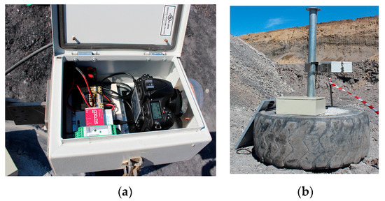
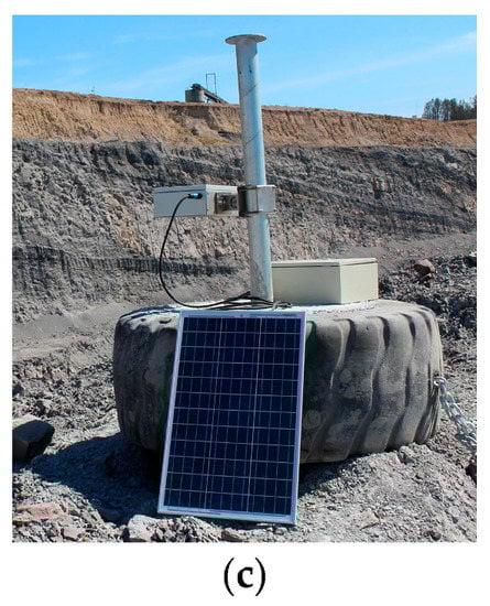
Figure 2.
The photogrammetric system: (a) inside view of the camera box, (b) left and (c) right unit installed in front of the highwall.
To allow the easy and flexible installation of the system, the camera box is supported by a mounting-arm which can be clamped to a cylindrical steel pole. The arm allows adjustment for tilt, roll and yaw, i.e., setting the orientation of the camera, by fine-tuning the regulation screws mounted on the arm itself. In the current application, the pole is cast into an old rubber tyre filled with concrete to act as a solid base (Figure 2b,c). The tyre has an overall diameter of 1.5 m and a width of 0.52 m, with the weight of the concrete filled tyre being about 2 tonnes. Such a solid foundation is required to limit the movements of the system that might occur due to wind gusts. Once the tyres and poles are set to the preferred location, the system components can be installed.
2.2. System Calibration and Installation
To ensure an accurate 3D reconstruction from the acquired images, all relevant geometric parameters of the optical system of each camera box need to be quantified. These include interior orientation (IO) and exterior orientation (EO) parameters. The IO parameters (principal distance, image coordinates of principal points, distortion parameters) control the reconstruction of the projection path of the rays through the optics. The EO parameters (camera position and orientation) are needed to orient the image reference space with respect to the object reference system. In photogrammetric applications, such parameters can generally be inferred indirectly through a bundle block adjustment (BBA) procedure using ground control points (GCP). However, if the depth of the scene is narrow and the image network consists of few cameras only (in this case just two), strong correlation between the parameters is expected, which can significantly increase unwanted systematic reconstruction errors. The use of several well-distributed GCPs is required to limit some of those unwanted systematic effects [47]. Given the mining environment where this system was installed, which entailed restricted access to the rock surface for safety reasons, the installation of physical GCPs located on the rock surfaces was not practical. The adoption of natural features as GCPs could also be considered [54]; however, their accurate identification in the image is often time consuming and potentially unreliable when the rock surface presents repeated or poorly distinguished patterns. To overcome these issues, the current study utilised a two-stage calibration procedure. Firstly, the IO parameters were estimated in a controlled environment. Secondly, a set of specific geometric parameters for the camera box, which allowed the identification of the site-specific EO parameters from a limited number of on-site measurements, was estimated in a separate calibration procedure. Both procedures are briefly described in the following paragraphs.
A rotating calibration panel with 72 coded targets is used to estimate the IO parameters (Figure 3a). Images of the panel are acquired from several positions around it. By rotating the camera around its optical axis (+90°, 0°, −90°) correlation between IO and EO parameters is prevented (Figure 3b). It should be noted that the protective glass located in front of the camera optics introduces additional distortions. Provided the thickness of the protective glass is small and the optical axis of the camera is approximately orthogonal to the glass surface, the additional distortion introduced by the glass itself is correctly modelled by the first radial term of Brown’s model [55]. Consequently, as long as the relative position between the camera and the protective glass do not change, the total distortion can be computed and accounted for. Hence, the calibration procedure must be performed with the camera box closed and with the camera fixed in its final operational position inside the box.
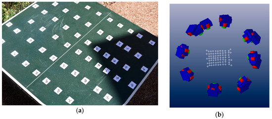
Figure 3.
(a) Example of an image of the calibration panel and (b) camera network used for the calibration procedure of the interior orientation parameters.
From a practical point of view, the calibration procedure can be tricky, even if the focal length of the cameras is not very long (50 mm). The camera lenses should be set to infinity, which requires considering a sufficient distance from the calibration panel to allow sharp pictures according to the depth of field of the lens. At the same time, to ensure an optimal calibration, the size of the calibration panel should be big enough to fill the entire picture frame. In this case a calibration panel of 1.40 × 1.6 m was used. If focusing at infinity during the panel calibration procedure is impractical, a site specific calibration procedure should be considered for the proper estimation of the IO parameters (especially for the principal distance).
The estimation of the EO parameters is based on pre-computed photogrammetric information and site-specific topographic measurements. First, the orientation of the camera with respect to the box that contains it is determined using a calibration procedure in a controlled environment. This consists of taking pictures of a calibration board, similar to the one used during the calibration of the IO parameters, and measuring the corresponding position of the camera box (i.e., the coordinates of the prism attached to the camera box) with a total station. The box is moved around the calibration board and the procedure is repeated several times to increase redundancy of the estimation model. Then, the EO parameters of each image are computed by space resection using the known GCPs. This allows for the estimation of the eccentricity vector, i.e., the vector between the measured location of the prism with respect to the camera perspective centre [56]. The last step needs to be conducted on site after installation of the system and it consists of measuring the coordinates of at least one GCP and the coordinates of each camera box with either a GNSS receiver or a total station. By combining this site-specific topological information with the pre-computed eccentricity vector, the absolute EO can be estimated [57]. In the case that no GCPs are provided, there is insufficient information to compute a rigid body transformation able to georeference the image block, which, in this case, consists only of tie-points. The available data (the location of one end of the eccentricity vector) allow partial EO parameter estimation (i.e., estimation of the scale only), which is sufficient if the rotations and actual position of the rock wall are not required. For instance, if only the size of the detaching blocks after a rock fall event is required, the arbitrariness of the reference system is not a limitation. However, a very simple way to overcome the issue of measuring GCPs is the installation of an inclinometer in one of the camera boxes. This allows direct measurement of the rotation that would fix the only free (rank-deficient) degree of freedom of the BBA procedure (i.e., the rotation around the line connecting the two ends of the eccentricity vector).
The installation procedure of the system can be summarised in eight main steps as follows:
- Positioning of the mounting poles and bases in the desired locations.
- Mounting of the camera boxes on to the poles.
- Connection of the camera boxes to their power supply (solar panel and batteries).
- Trial set-up of the camera boxes towards the section of the rock wall to be monitored.
- Acquisition of preliminary images from each camera to check overlap and focus.
- Final fixing of the orientation of the cameras by locking the regulation screws on the mounting bracket.
- Determination of the position of the camera boxes using a retroreflective prism or GNSS antenna mounted on the camera boxes (Figure 4). If full georeferencing is required, at least one GCP on the rock wall must also be measured.
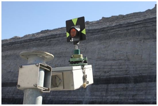 Figure 4. Retro-reflective prism mounted on the camera box at the time of the on-site installation of the system.
 - Acquisition of an initial stereo-pair for subsequent offline estimation of the site-specific EO parameters.
After the successful installation, the stereo-pair images were automatically acquired by the system by means of a Python script and the open-source library gPhoto2 (http://www.gphoto.org). The acquisition frequency and the acquisition parameters were defined in a trigger table, which is uploaded onto each system. Synchronicity of the system is guaranteed by a network time protocol (NTP) server which was accessed via the site WI-FI network. Once collected, the stereo-pair images were automatically uploaded onto a remote FTP server where they could be accessed for offline image processing.
2.3. Image Processing
Figure 5 shows the general workflow of the monitoring system. The main part of the image processing, including the dense matching and the 3D reconstruction of the DSM, is performed by a software package developed by the University of Parma, named Slope Monitor (SM). The images are always resampled, removing the distortion effects, at the beginning of the procedure to make the subsequent procedure easier and faster. In particular, a BBA of the first acquired stereo-pair is performed using the GCPs (if available) and the measured positions of the prism mounted on the camera and collected during the on-site survey. This procedure allows estimation of the site-specific EO parameters, which will be considered as fixed for all of the subsequent operations. At the end of the procedure, the DSM of the rock slope is reconstructed. This first DSM serves as the reference model for all subsequent image processing routines. It is used as an approximate 3D reconstruction of all subsequent acquisitions to accelerate the dense matching procedure, i.e., the initial DSM provides approximate information that allows the parallax search space to be limited during the matching procedure, which significantly reduces the computational cost of this step [58].
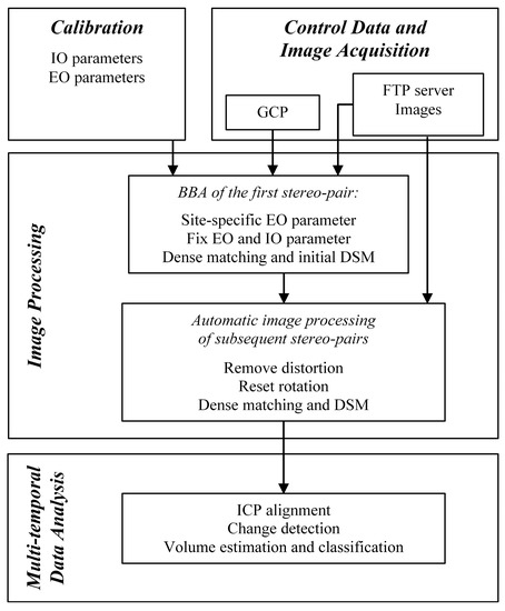
Figure 5.
General workflow of the monitoring system.
The general 3D reconstruction pipeline for any subsequent acquisition consists of three additional steps. First, as stated before, the incoming images are resampled according to the lens distortion values estimated during the IO parameter calibration procedure to remove image distortion. This makes all the subsequent image operations faster and allows for a simpler co-registration of image and 3D reconstruction data. Second, unwanted rotations of the cameras are corrected. Small unwanted variations in the camera attitude are very frequent (e.g., due to consolidation of the ground or working activity, such as blasting operations) and implicate a change of the EO parameters. Instead of computing a new set of EO parameters for each stereo-pair, which is impractical due to the intrinsic deficient rigidity of the image block geometry (see Section 2.2), the camera movement is assimilated to a small rotation around the camera centre (possible translations can be considered negligible). Its effect is then removed from the image using the procedure described in Roncella and Forlani [57]. Assuming the camera is rotating around its centre of perspective, a homographic transformation can track the movement of image plane features between the reference (i.e., the first, not rotated image) and the current image. Some corresponding points between the reference and the rotated image are used to compute such a transformation, which is subsequently applied to the rotated image. This means the new image is resampled to a condition ‘projectively’ equivalent to the initial configuration, i.e., the one that the initial computed EO parameters refer to.
Finally, the stereo-pair images are processed by a dense matching (DM) algorithm to obtain a 3D reconstruction of the rock face. Slope Monitor provides three DM processing options. The first two options are an in-house developed Least Squares matching procedure and a semi-global matching routine. Both techniques and their implementation are described in depth in Dell’Asta et al. [59]. The third option consists of interacting with the commercial software package Agisoft Photoscan, substituted in 2019 with Metashape [60], via Python scripting and using its matching routines. Whichever matching algorithm is used, at the end of the DM procedure a dense point cloud of the rock wall is obtained which is further triangulated to obtain a DSM. It should be noted that the point cloud is obtained by sampling the image points of the stereo pair on a regular grid. Therefore, the points are equally spaced in image projection.
2.4. Multi-Temporal Data Analysis
After processing of the stereo-pair images and the generation of the DSM of the new acquisitions, the multi-temporal data analysis can be performed (last task in Figure 5). The first step in this analysis consists of aligning the DSM of the new acquisition with the DSM of the previous stereo-pair using an Iterative Closest Point (ICP) algorithm. This is necessary to minimise the effect of possible systematic deformations of the DSM (e.g., due to small variation of the IO parameters between the acquisitions). The ICP is performed using the open-source package CloudCompare [61]. Then, a change detection algorithm similar to the one described in van Veen et al. [30] is applied to detected possible dislodged rocks. In particular, the cloud-to-mesh distance calculation algorithm of CloudCompare is used to calculate the distance between the two models. The next step consists of identifying potential rockfalls and eliminating changes detected due to noise and accuracy limitations in the DSM.
The minimum identifiable rockfall size depends on the ground sampling distance (GSD) and the expected measurement accuracy of the system. The GSD of an image can be calculated as in equation [1]:
where is the object distance (distance from the camera to the rock face), is the pixel size of the sensor (for the Nikon D810 it corresponds to 4.89 µm/pixel) and is the focal length of the lens (50 mm). The expected depth accuracy can be estimated by equation [2,62]:
where is the measurement precision of the image coordinates (assumed to be ±1 pixel [63]) and is the base length (i.e., distance between the two cameras). Three criteria are used to identify effective rockfalls. First, it is assumed that areas with distances between the models bigger than are potential rockfall. Second, the number of vertices in each identified area is checked and only areas with more than 25 vertices are considered. This corresponds to an area of about 5 × 5 the GSD. All other areas are considered noise and disregarded. Figure 6 shows an example of a segment of the rock face after change detection with areas indicating potential rockfalls. The final criterion is a visual inspection on the 3D model and the images of the identified area by a trained operator. If the visual inspection confirms that the area is indeed a missing block, the relevant vertices of both models (reference model and new model) are merged, exported and labelled for further post-processing.
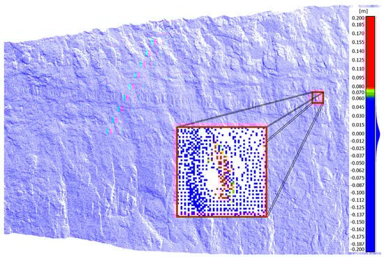
Figure 6.
Segmentation of the missing rock that has been dislodged for further calculation of the volume. Changes (i.e., maximum distances between the two compared point clouds in metres) are highlighted in red. Blue indicates no change.
The final step of the analysis consists of determining volume and shape characteristics of all identified rockfalls. This is obtained by analysing the labelled exported point clouds that define the blocks. First, the point cloud is analysed to identify the axis that corresponds to the greatest moment of inertia. Then, the point cloud is transformed (i.e., rigid rotation and translation) into a new local reference system with origin in the centre of gravity and with coordinate axes aligned with the principal axes of inertia, with the z axis defined as the principal axis corresponding to the highest moment of inertia. According to Bonneau et al. [64], the use of the side lengths of the bounding box of a point cloud can result in an overestimation of the block volume and inaccurate shape characterisation. Hence, the block volume is calculated by rasterising the point cloud (raster size equal to GSD), considering the points from the reference and new model separately, and using a mapping plane orthogonal to the local z direction. The volume of the block is given by summing the volumes between the reference and the comparison cell of the two rasters. Finally, the principal dimensions of the block corresponding to the longest (a), intermediate (b) and shortest (c) orthogonal axes are estimated from the point cloud of the block. The shape classification proposed by Sneed and Folk [65] based on the ratios b/a, c/a and (a-b)/(a-c) is used. Although initially developed for pebbles, it is a very common classification scheme for rockfall fragments [30,64]. The ratios are plotted on a ternary diagram (Figure 7) where blocks can be classified into 10 different shape classes: C (compact), CP (compact-platy), CB (compact-bladed), CE (compact-elongated), P (platy), B (bladed), E (elongated), VP (very platy), VB (very bladed), VE (very elongated).
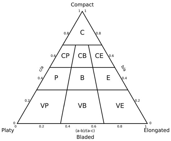
Figure 7.
Triangular shape classification diagram proposed by Sneed and Folk (1958) with 10 classes: C (compact), CP (compact-platy), CB (compact-bladed), CE (compact-elongated), P (platy), B (bladed), E (elongated), VP (very platy), VB (very bladed), VE (very elongated).
3. System Validation
An assessment of the accuracy and repeatability of the DSM generated by the system was conducted in an abandoned sandstone quarry at Pilkington Reserve in Newcastle (NSW, Australia). The quarry walls expose very thickly bedded, medium grained sandstones with sub-vertical joint spacing of 2 to 6 m in two primary directions. The majority of exposed faces are smooth joint surfaces, with smaller areas where excavation has broken through intact rock. The exposed rock face is about 80 m long and has an average height of about 6 m. A section of the wall 6 m high and 13 m long was considered for validating the system, as shown in Figure 8.
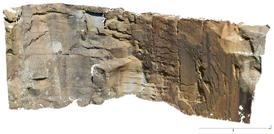
Figure 8.
Digital surface model of the portion of the wall considered in the analysis excluding the vegetated areas.
The photogrammetric system was set up on tripods pointing to the wall. The cameras were placed 20 m away from the wall with a base length of 8 m in a slightly convergent geometric configuration. The resulting GSD according to Equation [1] is approximately 1.96 mm/pixel. The depth accuracy according to Equation [2] is about 5 mm (2.5 GSD). Although, in actual operational conditions, the monitoring system would most likely be installed much further from the face to frame a much wider rock wall area (and the GSD would be much greater), the Pilkington site was considered the best option for system validation given its easy and safe accessibility and the availability of an accurate reference TLS point cloud [54]. In the following analysis, all the validation results will be presented both in metric (mm) and GSD proportional units, so that relevant results can be easily transferred to other image blocks with similar geometric configuration (i.e., ) but with much greater distances from the object.
A time window from 3:50 pm to 4:50 pm was considered and images were taken every 15 min, resulting in a total of five acquisitions (3:50 pm, 4:05 pm, 4:20 pm, 4:35 pm, 4:50 pm). The acquisition parameters such as ISO, aperture and shutter speed were the same for all acquisitions and for both cameras.
Dense point clouds with an average density of 8.4 points/cm2 were generated for each acquisition period, using the two DM algorithms implemented in Slope Monitor (SM) and the one implemented in Agisoft PhotoScan (PS). Note that since the Least Squares Matching and Semi-global Matching algorithms implemented in SM provided basically identical results, only results from the Least Squares Matching algorithm are presented. The obtained DSMs were then compared with the reference TLS data. Considering the photogrammetric precision of the point coordinates (about 5 mm), assuming Equation [2] can also be applied for the estimation of the DSM precision, and the TLS point cloud accuracy (about 4 mm), from the comparison of the two data sets a root mean squared error (RMSE) of the distances between the two reconstructions of about 6.4 mm (3.3 GSD) should be expected. It should be noted that, according to general requirements for accuracy assessment (see for instance [66]) the reference data should be at least three times more precise than the expected precision of the tested dataset. However, at this distance, photogrammetry and laser scanning provide similar precision. Table 1 provides a summary of the accuracy check between the TLS data and all photogrammetric models. The data indicate that the models generated with SM give results very close to the expected accuracy if not slightly better whereas PS seems to give results with an accuracy slightly above the expected. Nevertheless, both results are not far off the expected accuracy of 5.8 mm and the results generated with SM are about 20% better than expected.

Table 1.
Summary of the accuracy check between the TLS data and the photogrammetric models obtained with SlopeMonitor (SM) and Agisoft PhotoScan (PS).
It should be noted that the comparison between photogrammetric and TLS data might be affected by systematic errors or deformations of one or both the data sources. However, as far as a change detection application is concerned, where per-period discrepancies rather than absolute coordinates have to be identified, systematic effects should be reciprocally cancelled in the comparison. For this purpose, and as an additional validation check, each of the four models collected at 4:05 pm, 4:20 pm, 4:35 pm and 4:50 pm was also compared to the first photogrammetric model (3:50 pm). Table 2 shows the comparisons of the RMSE of the distances obtained for both software packages. Results show that the RMSE of the distances for SM is below 1 GSD whereas it is almost 2 GSD for PS.
Table 2.
Summary of the repeatability check of the photogrammetric models obtained with SlopeMonitor (SM) and Agisoft PhotoScan (PS).
The results of the comparisons conducted on the trial test highlight the capability of the system to produce accurate and repeatable 3D models. Indeed, the image processing algorithm implemented in the photogrammetric system generates accurate DSMs as per the expected precision calculated by Equation [2]. Nevertheless, it seems that SM provides slightly better results than PS and hence, in all the following analyses, only the generated DSMs with SM are used.
4. Application
The system was deployed in a coal mine located in the Hunter Valley (New South Wales, Australia) to evaluate its usefulness in obtaining temporal-spatial data on the occurrence of rockfall events. As rockfall events from rock faces are both rapid and random, it is impractical to capture data on the size, shape and timing of events by simple observation, and so, such data are relatively scarce. The system described here has great potential to now make such data accessible.
4.1. Site Description
The studied highwall exposes a 50 m high section of the Permian Wittingham Coal Measures containing the upper and lower Liddell coal seams. The upper ~10 m comprises the weathered zone, where the geological materials (including the upper Liddell seam) are highly to extremely weathered and their texture is extensively degraded (soil-like). Hence, the upper 10 m of the wall was cut back to a low angle (45° slope angle) and a bench was formed at its base, at the top of the unweathered material. This upper part is not considered in the analysis.
The 70 m long, studied section of the main highwall face, striking 75–255°, was formed by presplit blasting at an average slope angle of 74°, and it comprises a 26 m thick stratigraphic interval of predominantly fine to medium sandstones and siltstone, with minor claystone, as shown in Figure 9a. The ~1.4 m thick lower Liddell coal seam passes through the upper half of the main face (below the bench), dipping to the south (left to right) at about 7°. Sandstone comprises about 60% of the total vertical thickness, with siltstones comprising about 35% and coal the remaining 5%, although the proportions of sandstone and siltstone do vary across the face due to the dip of the strata and some lateral lithology changes. The siltstones mostly occur directly above and below the coal seam, with sandstones occurring at the top and bottom of the section. The rock face is quite heavily fractured from a combination of closely spaced joints (up to five sets are present) and blast damage. The face had been exposed and had stood without modification for a period of 14 months prior to this study so that a great many rockfalls had already occurred, as was evident from the build-up of debris at its base.
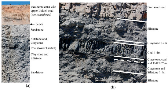
Figure 9.
(a) Full geological sequence with (b) lithological detail adjacent to coal seam.
Of specific interest are the lithological characteristics immediately above and below the coal seam (Figure 9b) which were logged in detail by the exploration geologists on the site as claystones (from internal mine records), with the underlying claystone recognised to have some tuffaceous content, which often corresponds to a high smectite content [67,68,69]. Also of interest is the distinctive fracturing in the coal seam, which is only weakly laminated, but which displays clean, closely spaced jointing (cleating) that is continuous throughout the entire thickness of the seam (Figure 9a).
4.2. System Installation and Set-Up Validation
The photogrammetric system described in Section 2 was installed in front of the rock wall and data was collected for 46 days. The two units were positioned on top of a berm of waste rock located opposite the wall at an approximate distance from the wall of around 110 m (given the variation of the wall geometry within the monitored section, the distance Z varied between 100 and 120 m). The two cameras had a base length of 28 m and they were orientated in a slight convergent pose to ensure maximum overlap. The GSD and the depth precision were 1.1 cm and 4.2 cm, respectively. Figure 10a,b show the left and right images of the portion of rock wall captured by the left and right camera, respectively. A reflector prism was set up on each unit to measure its precise position by means of a total station. As pointed out in Section 2.2, a single GCP is generally sufficient to determine the absolute orientation of the image block. Nevertheless, in this case, 15 natural GCPs widely distributed on the surface of the wall were surveyed on the rock face using a reflectorless total station (Leica MS60) shortly after the system installation. Redundancy in the number of GCPs was required as natural features can sometimes be unreliable as GCPs (i.e., they can easily be misidentified during image orientation). In addition, a validation with an external dataset (e.g., a TLS scan as in this case) requires additional effort (e.g., more GCPs). In fact, particularly with the considered acquisition set-up (i.e., long focal length, single stereo-pair) possible correlations between orientation parameters might introduce unwanted deformation in the 3D reconstruction (as pointed out in Section 3). As long as the comparison is performed on DSMs acquired with the same system, this possible systematic deformation reciprocally cancels out, but if the photogrammetric models are to be compared to a TLS point cloud, such deformation should be limited using more GCPs.
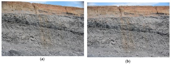
Figure 10.
Example of (a) left and (b) right captured by the monitoring system.
Images acquired at 12:00 pm and 2:00 pm during the first 11 days of monitoring (period between 8 February 2018 and 21 February 2018) were adopted to assess the accuracy and repeatability of the DSMs generated by the system. Different lighting conditions were experienced with prevalent sunny days, but also with cloudy and hazy days. Some stereo-pairs had to be excluded from the analysis due to issues with data transmission (i.e., some images were corrupted). A total of 21 stereo-pairs were considered in the analysis.
The data accuracy was assessed by comparing the point clouds with a TLS scan (Leica C10) acquired on the day of the installation. The TLS measurement noise (ca. 4 mm) is considered negligible compared to the expected system accuracy of 4.2 cm estimated using Eq. [2]. The TLS point cloud was triangulated and the mesh compared to the point clouds obtained using SM. Two different matching resolution levels were used with the main difference being the number of generated points (an average 1.25 million vs. 4.3 million points per point cloud). The comparisons showed similar results for all the point clouds with an average RMSE of the distances from the reference (TLS) DSM of 2.6 cm (2.4 GSD) for both levels of resolution. Overall, the RMSE varied from 2.4 to 2.8 cm. This indicated that the results were more accurate than expected, and similarly to Section 3, highlighted the excellent performance of the system and the implemented algorithms under real conditions. Since the accuracy seemed to be much higher than expected, for block fall identification (see next section) the maximum RMSE observed (2.8 cm), rather than the expected precision evaluated using equation [2] (4.2 cm), was adopted for computing the change detection threshold.
A repeatability analysis was also conducted as a relevant indicator of the system’s performance for change detection of rockfall events. For this purpose, all point clouds were compared to the first one (12:00 pm of the first day). In this case, the comparison illustrated the influence of the matching resolution level. The average RMSE of the distances for the higher resolution models was 2.1 cm, ranging from 1.4 (same day 2:00 pm) to 2.4 cm (last day). The values for the lower resolution models were slightly higher with an average RMSE of 2.2 cm (2 GSD) and a range from 1.5 to 2.8 cm. As a final check, the same analysis was performed separately for the point clouds generated with the images acquired on 12:00 pm and 2:00 pm. The results of the RMSE did not change, indicating that small variations in the lighting conditions do not affect the repeatability of the results.
4.3. Multi-Temporal Data Analysis
The acquired images were analysed to evaluate the effectiveness of the system for change detection and volume estimation in the context of the temporal and spatial occurrence of rockfall events. The data were aggregated to correspond to four specific periods between February and March 2018, defined according to the climatic events observed in that period, so that the influence of the significant rainfalls (or not) on the detachment/dislodgement of rocks from the rock face could be considered. The defined study periods (A1 to A4) are indicated on the rainfall records shown in Figure 11. Period A1 (11 days) is characterised by an absence of rainfall (dry); period A2 (17 days) recorded three major (>10 mm) and two minor rainfall events (total of 99 mm; wet); period A3 (8 days) is a dry period immediately following the rain (short-term dry); and period A4 (10 days) is a subsequent dry period (long-term dry). Table 3 shows the date and rainfall details for the four periods (A1 to A4).
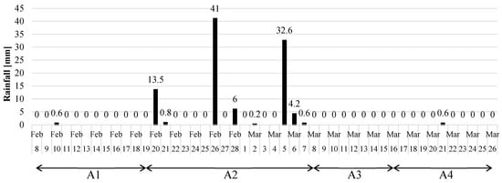
Figure 11.
Rainfall recorded with indication of the selected monitoring periods used in the comparison.
Table 3.
Key information related to the monitoring periods.
The images used to reconstruct 3D surfaces for the selected periods were consistently those collected at midday in order to have similar lighting conditions and to assure good quality images. Rockfalls during the period were identified at locations where there was a significant difference between the 3D surface model at the beginning (Reference Model) and end (Comparison Model) of the period. The change detection procedure used involved subtraction of successive 3D models to look for significant differences between the two surface models. The threshold for the change detection algorithm was set to 5.6 cm (twice the maximum RMSE observed), i.e., only areas with distances bigger than 5.6 cm were considered as potential rockfall events. The value was set in accordance with the level of accuracy estimated in Section 4.2. Then, by exploring the extent of the surfaces over which a discrepancy greater than 6 cm prevailed, both the volume and the shape of the missing block could be estimated. The lithology of the block was determined by cross referencing its position with the distribution of lithologies exposed in the wall.
5. Results and Discussion
Figure 12 shows the size and position of rockfall events (significant changes in the 3D surface models during a period) recorded during the study. It is clear that more and larger rockfalls occurred during periods A2 and A4, whilst fewer, smaller rockfalls occurred during periods A1 and A3. It is also evident that rockfalls are more frequent from, and adjacent to the coal seam in the middle of the face, and less frequent from the top and bottom of the face.
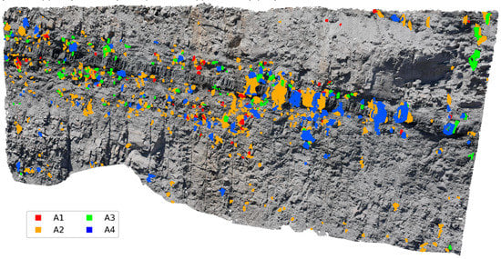
Figure 12.
Sites of individual rockfall detections on the studied wall, colour-coded to indicate the period in which they occurred.
Table 4 is a summary of inferred rockfall events, as a function of period, size and lithology. Note that the frequency values are normalised on a weekly basis, so they are comparable regardless of the differing period lengths. The quantitative data corroborate the trends observed in Figure 12; that the wet and long-term dry periods have higher rockfall event frequency, and larger maximum block volumes, than the initial dry and short-term dry periods. Furthermore, the increased event frequency in the wet and long-term dry periods is evident not only in the total for all layers, but also for each individual lithology.
Table 4.
Summary of the recorded information at the study site.
On first consideration, it may seem inconsistent that very wet and very dry conditions should both promote greater rockfall frequencies than less extreme conditions; however, the high level of specific detail in the data from this study allows for a detailed consideration of how this happens to be. Looking closely at the data in Table 4, it is apparent that the highest frequency of events occurs in the siltstone/claystone units. There are argillaceous materials which are moderately to highly clay-rich. This makes them prone to degradation, slaking and swelling when exposed to free water, and when exposed to intense drying after being wetted. During the wet period A2, combined actions of physical erosion, swelling and spalling destabilise fragments of these argillaceous rocks, allowing them to fall. Then, when drying occurs, the same materials shrink, causing fractures to propagate and their mechanical support to reduce, also promoting their destabilisation. As might be expected, the effects of these mechanisms increase as the severity of drying increases. Hence, periods without rain but also without intense drying are most favourable to preserve stability in these units.
Figure 13 presents the volume–frequency relationship for each lithology considering the whole monitoring period, and it confirms that small and very small fragments of siltstone and claystone are the most common rockfall event. It also shows that detachments of these materials in volumes greater than 0.25 m3 did not occur at any time during the study. By contrast, detachments of coal fragments are much less frequent, but when they occur, they are relatively much more likely to be substantially larger fragments. To explain this, it is necessary to re-examine Figure 9 which shows the precarious relationship between the coal seam and the water-sensitive lithologies of siltstone, and especially the claystones [70]. From Figure 9, it is evident that the claystone units either side of the coal seam are prone to preferential spalling and loss, causing the coal seam to become unsupported, particularly at its base (note the shadows caused by the overhanging coal seam at its base in Figure 9b). Unlike the siltstones and claystones which fracture and spall readily [71,72], the coal seam is coherent, except for the pervasive vertical cleats. Hence, when a portion of the coal becomes destabilised, it detaches as a prism or slice of coal, potentially through the full thickness of the seam.
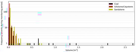
Figure 13.
Volume–frequency (total number of events during the monitoring period) relation of rockfall events per material recorded over all monitoring periods.
Figure 14 further considers the volume frequency data of Figure 13, but now with comparison of behaviours in the four periods A1–A4, and it reveals that there is a consistent but different relationship for each period when plotted in log-log space. The data confirm that periods A2 and A4 have similar volume frequency behaviour, and the frequency of events in these periods is very much greater than in periods A1 and A3.
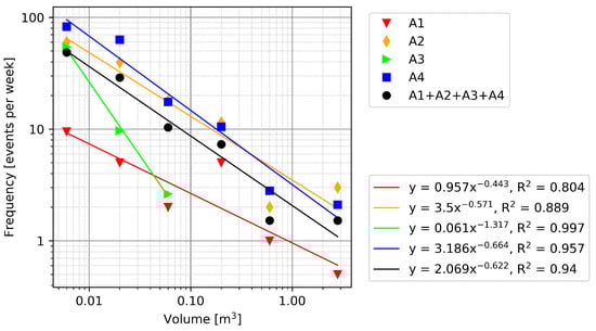
Figure 14.
Volume–frequency (normalised by week) diagram for the study site.
As described previously, the system detailed in this paper allows not only for the detection of detachments, but also estimates of their size and shape. Figure 15 shows the detachments for periods A1 to A4 plotted on the shape classification diagram of Sneed and Folk [65]. The size of fragments has been grouped into four categories, indicated by proportionately larger symbols, and the lithology of fragments is indicated by different colours.
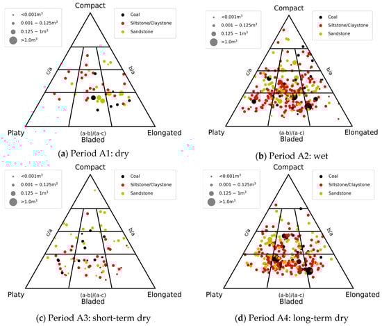
Figure 15.
Rockfall events recorded during each monitoring period categorised by shape, size and material for periods (a) A1, (b) A2, (c) A3 and (d) A4.
Again, it is evident that periods A2 and A4 display the greatest numbers of individual detachments, and that detachments in siltstone and claystone are more likely, whilst larger detachments are more likely to occur from the coal seam. Siltstone/claystone detachments larger than 0.125 m3 are rare, whereas detachments larger than 0.125 m3 are most likely to be coal blocks, and detachments greater than 1 m3 were only observed from the coal seam.
Figure 15 indicates that few of the detachments in any lithology were inclined to be compact, and, in particular, detachments of blocks of coal tended to be either bladed or elongated. Further re-examination of Figure 9 provides an explanation for this. As the Lower Liddell coal seam is a single bed of coal with only weakly developed laminations, and pervasive vertical cleating developed in two orthogonal directions, it has a tendency to detach slices and prisms over its full thickness (~1.4 m) in a single event, when destabilised by the fretting of the claystone from its base. This explains both the larger size and elongated shape of the coal detachments. By contrast, the siltstone and claystone tend to degrade to produce smaller flakes and spalls, which also tend not to be compact, but which are likely to be smaller, and just as likely to be platy as they are to be bladed or elongated. Sandstone, however, is more likely to produce blocks which are joint-controlled (refer also to Figure 10), and hence, are more likely to be compact, and this is evident in the detachments of all periods but particularly in A3.
6. Conclusions
An autonomous terrestrial stereo-pair photogrammetric monitoring system was developed to collect volumes and frequency of rocks detaching from sub-vertical rock faces in surface mining environments, and it is described in this paper. The system was specifically developed to provide a low-cost and effective solution that can be efficiently applied to areas often constrained by accessibility and safety and to account for the rough environmental conditions that are typical of mining operations. The total cost of the system including software is about AUD 20,000, which is considerably less compared to alternative monitoring systems such as LiDAR and GB InSAR. The system collects synchronised stereo-pair images at different periods that are readily used to produce accurate DSMs of the rock surfaces that can support automatic detection of detachments and surface movements during defined periods of observation. A thorough validation campaign, comprising application to a convenient test site and deployment of the system to monitor a highwall during actual mining operations in an active mine, demonstrated that the system provides reliable and accurate results over time. In the example presented in this paper, the interval between images was chosen to examine the impact of environmental conditions on rockfall frequency. There is no reason, however, why a much shorter interval could not be chosen to observe (for example) the rocks detached during a single mine blasting event.
The system is confirmed as an effective means of achieving difficult-to-obtain data on rockfall size-shape-frequency, with the capacity to reliably detect detached blocks as small as 200 cm3 in volume. Clear and explicable trends are evident from the data acquired despite the relatively short data record, which was limited by the rapidly changing physical environment of the operating coal mine. It is expected that a longer data record would lead to more and clearer trends in rockfall event likelihood to be established.
In interpreting the data in this study, it is important to appreciate that the data strictly describes the size and shape of detached rock masses, which do not necessarily equate to the size and shape of the blocks of rock that fell. As the detachments were inferred from the difference between 3D models at the beginning and end of each period, it is possible that some detachments occurred as progressive events over a period of days, rather than as a single event. It is also likely that some of the detachments, whilst a single event, produced many smaller blocks simultaneously which fell independently, rather than a single larger block. In addition, given the size of the wall, most of the blocks fragmented during their fall or at impact with the mine floor, making measurements of blocks on the floor irrelevant. These remain details to be researched.
An obvious enhancement through future work would be to fully automate the change detection procedure, which at this time requires intervention by a human operator. Full automation would significantly reduce human interaction [and subjectivity] in the identification of rock fall events. The addition of fully automated processing, to accommodate incremental comparisons of successive images at intervals as short as 15 min, would allow a more detailed correlation of rockfalls to rainfall both as and after it occurs, as well as to different times of the day, allowing other factors, such as exposure to direct sunlight, etc., to be considered.
Author Contributions
Conceptualization, A.G., K.T. and R.R.; methodology, R.R., K.T. and S.F.; software, R.R., F.D. and M.S.; validation, M.S., K.T., R.R., A.G. and F.D.; formal analysis, M.S., K.T. and R.R.; investigation, A.G., R.R., K.T., S.F. and M.S.; resources, S.B., and A.G.; writing—original draft preparation, M.S., A.G., K.T. and R.R.; writing—review and editing, A.G., S.F., R.R., K.T.; supervision, A.G. and R.R.; project administration, A.G.; funding acquisition, A.G., R.R., S.F. and S.B. All authors have read and agreed to the published version of the manuscript.
Funding
This research was funded by the Australian Research Council (grant number LP160100370).
Acknowledgments
The authors would like to acknowledge Glencore for providing the test site and personnel for the assistance during the system installation and Ecometer s.n.c (www.ecometer.it) for providing materials.
Conflicts of Interest
The authors declare no conflict of interest. The funders had no role in the design of the study; in the collection, analyses, or interpretation of data; in the writing of the manuscript, or in the decision to publish the results.
References
- Giacomini, A.; Thoeni, K.; Lambert, C.; Booth, S.; Sloan, S.W. Experimental study on rockfall drapery systems for open pit highwalls. Int. J. Rock Mech. Min. Sci. 2012, 56, 171–181. [Google Scholar] [CrossRef]
- Ferrari, F.; Giacomini, A.; Thoeni, K. Qualitative Rockfall Hazard Assessment: A Comprehensive Review of Current Practices. Rock Mech. Rock Eng. 2016, 49, 2865–2922. [Google Scholar] [CrossRef]
- Royán, M.J.; Abellán, A.; Jaboyedoff, M.; Vilaplana, J.M.; Calvet, J. Spatio-temporal analysis of rockfall pre-failure deformation using Terrestrial LiDAR. Landslides 2014, 11, 697–709. [Google Scholar] [CrossRef]
- Macciotta, R.; Hendry, M.; Cruden, D.M.; Blais-Stevens, A.; Edwards, T. Quantifying rock fall probabilities and their temporal distribution associated with weather seasonality. Landslides 2017, 14, 2025–2039. [Google Scholar] [CrossRef]
- Terzaghi, K. Stability of steep slopes on hard unweathered rock. Geotechnique 1962, 12, 251–270. [Google Scholar] [CrossRef]
- Bjerrum, L.; Jørstad, F.A.; Jørstad, F.A. Stability of Rock Slopes in Norway; Norges Geotekniske Institute: Oslo, Norway, 1968. [Google Scholar]
- Peckover, F.L. Treatment of Rock Falls on Railway Lines; American Railway Engineering Association: Montreal, QC, Canada, 1972. [Google Scholar]
- Delonca, A.; Gunzburger, Y.; Verdel, T. Statistical correlation between meteorological and rockfall databases. Nat. Hazards Earth Syst. Sci. 2014, 14, 1953–1964. [Google Scholar] [CrossRef]
- Collins, B.D.; Stock, G.M. Rockfall triggering by cyclic thermal stressing of exfoliation fractures. Nat. Geosci. 2016, 9, 395–400. [Google Scholar] [CrossRef]
- Macciotta, R. Review and latest insights into rock fall temporal variability associated with weather. Proc. Inst. Civ. Eng. Geotech. Eng. 2019, 172, 556–568. [Google Scholar] [CrossRef]
- Krautblatter, M.; Moser, M. A nonlinear model coupling rockfall and rainfall intensity based on a four year measurement in a high Alpine rock wall (Reintal, German Alps). Nat. Hazards Earth Syst. Sci. 2009, 9, 1425–1432. [Google Scholar] [CrossRef]
- Macciotta, R.; Martin, C.D.; Edwards, T.; Cruden, D.M.; Keegan, T. Quantifying weather conditions for rock fall hazard management. Georisk 2015, 9, 171–186. [Google Scholar] [CrossRef]
- Jaboyedoff, M.; Oppikofer, T.; Abellán, A.; Derron, M.H.; Loye, A.; Metzger, R.; Pedrazzini, A. Use of LIDAR in landslide investigations: A review. Nat. Hazards 2012, 61, 5–28. [Google Scholar] [CrossRef]
- Abellán, A.; Oppikofer, T.; Jaboyedoff, M.; Rosser, N.J.; Lim, M.; Lato, M.J. Terrestrial laser scanning of rock slope instabilities. Earth Surf. Process. Landf. 2014, 39, 80–97. [Google Scholar] [CrossRef]
- Scaioni, M.; Longoni, L.; Melillo, V.; Papini, M. Remote Sensing for Landslide Investigations: An Overview of Recent Achievements and Perspectives. Remote Sens. 2014, 6, 9600–9652. [Google Scholar] [CrossRef]
- Jaboyedoff, M.; Ornstein, P.; Rouiller, J.-D. Design of a geodetic database and associated tools for monitoring rock-slope movements: The example of the top of Randa rockfall scar. Nat. Hazards Earth Syst. Sci. 2004, 4, 187–196. [Google Scholar] [CrossRef]
- Bertacchini, E.; Capra, A.; Castagnetti, C.; Corsini, A. Atmospheric corrections for topographic monitoring systems in landslides. In Proceedings of the FIG Working Week 2011, Marrakesh, Morocco, 18–22 May 2011; pp. 1–15. [Google Scholar]
- Ferrero, A.M.; Forlani, G.; Roncella, R.; Voyat, H.I. Advanced Geostructural Survey Methods Applied to Rock Mass Characterization. Rock Mech. Rock Eng. 2009, 42, 631–665. [Google Scholar] [CrossRef]
- Delacourt, C.; Allemand, P.; Berthier, E.; Raucoules, D.; Casson, B.; Grandjean, P.; Pambrun, C.; Varel, E. Remote-sensing techniques for analysing landslide kinematics: A review. Bull. Soc. Geol. Fr. 2007, 178, 89–100. [Google Scholar] [CrossRef]
- Casagli, N.; Catani, F.; Del Ventisette, C.; Luzi, G. Monitoring, prediction, and early warning using ground-based radar interferometry. Landslides 2010, 7, 291–301. [Google Scholar] [CrossRef]
- Travelletti, J.; Delacourt, C.; Allemand, P.; Malet, J.P.; Schmittbuhl, J.; Toussaint, R.; Bastard, M. Correlation of multi-temporal ground-based optical images for landslide monitoring: Application, potential and limitations. ISPRS J. Photogramm. Remote Sens. 2012, 70, 39–55. [Google Scholar] [CrossRef]
- Casagli, N.; Frodella, W.; Morelli, S.; Tofani, V.; Ciampalini, A.; Intrieri, E.; Raspini, F.; Rossi, G.; Tanteri, L.; Lu, P. Spaceborne, UAV and ground-based remote sensing techniques for landslide mapping, monitoring and early warning. Geoenviron. Disasters 2017, 4, 1–23. [Google Scholar] [CrossRef]
- Michoud, C.; Bazin, S.; Blikra, L.H.; Derron, M.H.; Jaboyedoff, M. Experiences from site-specific landslide early warning systems. Nat. Hazards Earth Syst. Sci. 2013, 13, 2659–2673. [Google Scholar] [CrossRef]
- Sturzenegger, M.; Keegan, T.; Wen, A.; Willms, D.; Stead, D.; Edwards, T. LiDAR and discrete fracture network modeling for rockslide characterization and analysis. In Engineering Geology for Society and Territory; Springer: Berlin/Heidelberg, Germany, 2015; Volume 6, pp. 223–227. [Google Scholar]
- Guidelines for Slope Performance Monitoring; Sharon, R., Eberhardt, E., Eds.; CSIRO Publishing: Clayton, Australia, 2020; ISBN 9781486310999. [Google Scholar]
- Farina, P.; Leoni, L.; Babboni, F.; Coppi, F.; Mayer, L.; Ricci, P. IBIS-M, an Innovative Radar for Monitoring Slopes in Open-Pit Mines. In Proceedings of the Interrnational Symposium on Rock Slope Stability in Open Pit Mining and Civil Engineering, Vancouver, BC, Canada, 18–21 September 2011. [Google Scholar]
- Severin, J.; Eberhardt, E.; Leoni, L.; Fortin, S. Development and application of a pseudo-3D pit slope displacement map derived from ground-based radar. Eng. Geol. 2014, 181, 202–211. [Google Scholar] [CrossRef]
- Abellán, A.; Calvet, J.; Vilaplana, J.M.; Blanchard, J. Detection and spatial prediction of rockfalls by means of terrestrial laser scanner monitoring. Geomorphology 2010, 119, 162–171. [Google Scholar] [CrossRef]
- Ferrero, A.M.; Migliazza, M.; Roncella, R.; Segalini, A. Rock cliffs hazard analysis based on remote geostructural surveys: The Campione del Garda case study (Lake Garda, Northern Italy). Geomorphology 2011, 125, 457–471. [Google Scholar] [CrossRef]
- van Veen, M.; Hutchinson, D.J.; Kromer, R.; Lato, M.; Edwards, T. Effects of sampling interval on the frequency—magnitude relationship of rockfalls detected from terrestrial laser scanning using semi-automated methods. Landslides 2017, 14, 1579–1592. [Google Scholar] [CrossRef]
- Lato, M.; Diederichs, M.S.; Hutchinson, D.J.; Harrap, R. Optimization of LiDAR scanning and processing for automated structural evaluation of discontinuities in rockmasses. Int. J. Rock Mech. Min. Sci. 2009, 46, 194–199. [Google Scholar] [CrossRef]
- Oppikofer, T.; Jaboyedoff, M.; Pedrazzini, A.; Derron, M.H.; Blikra, L.H. Detailed DEM analysis of a rockslide scar to characterize the basal sliding surface of active rockslides. J. Geophys. Res. Earth Surf. 2011, 116, 1–22. [Google Scholar] [CrossRef]
- Klappstein, B.; Bonci, G.M.W.; Maston, W. Implementation of Real Time Geotechnical Monitoring at an Open Pit Mountain Coal Mine, Western Canada. In Proceedings of the International Multidisciplinary Symposium UNIVERSITARIA SIMPRO, Petrosani, Romania, 10–11 October 2014; pp. 250–262. [Google Scholar]
- Kromer, R.A.; Abellan, A.; Hutchinson, D.J.; Lato, M.; Chanut, M.-A.; Dubois, L.; Jaboyedoff, M. Automated Terrestrial Laser Scanning with Near Real-Time Change Detection—Monitoring of the Séchilienne Landslide. Earth Surf. Dyn. Discuss. 2017, 1–33. [Google Scholar] [CrossRef]
- Kromer, R.A.; Rowe, E.; Hutchinson, J.; Lato, M.; Abellán, A. Rockfall risk management using a pre-failure deformation database. Landslides 2018, 15, 847–858. [Google Scholar] [CrossRef]
- Williams, J.G.; Rosser, N.J.; Hardy, R.J.; Brain, M.J.; Afana, A.A. Optimising 4-D surface change detection: An approach for capturing rockfall magnitude-frequency. Earth Surf. Dyn. 2018, 6, 101–119. [Google Scholar] [CrossRef]
- Casson, B.; Delacourt, C.; Baratoux, D.; Allemand, P. Seventeen years of the “La Clapière” landslide evolution analysed from ortho-rectified aerial photographs. Eng. Geol. 2003, 68, 123–139. [Google Scholar] [CrossRef]
- Liu, W.C.; Huang, W.C. Close range digital photogrammetry applied to topography and landslide measurements. Int. Arch. Photogramm. Remote Sens. Spat. Inf. Sci.—ISPRS Arch. 2016, 41, 875–880. [Google Scholar] [CrossRef]
- Thoeni, K.; Santise, M.; Guccione, D.E.; Fityus, S.; Roncella, R.; Giacomini, A. Use of low-cost terrestrial and aerial imaging sensors for geotechnical applications. Aust. Geomech. J. 2018, 53, 101–122. [Google Scholar]
- Sturzenegger, M.; Stead, D. Close-range terrestrial digital photogrammetry and terrestrial laser scanning for discontinuity characterization on rock cuts. Eng. Geol. 2009, 106, 163–182. [Google Scholar] [CrossRef]
- Lato, M.J.; Vöge, M. Automated mapping of rock discontinuities in 3D lidar and photogrammetry models. Int. J. Rock Mech. Min. Sci. 2012, 54, 150–158. [Google Scholar] [CrossRef]
- Thoeni, K.; Irschara, A.; Giacomini, A. Efficient photogrammetric reconstruction of highwalls in open pit coal mines. In Proceedings of the 16th Australasian Remote Sensing and Photogrammetry Conference Proceedings, Melbourne, Australia, 25 August–1 September 2012; pp. 85–90. [Google Scholar]
- Tannant, D. Review of Photogrammetry-Based Techniques for Characterization and Hazard Assessment of Rock Faces. Int. J. Geohazards Environ. 2015, 1, 76–87. [Google Scholar] [CrossRef]
- Travelletti, J.; Malet, J.-P.; Schmittbuhl, J.; Toussaint, R.; Bastard, M. Multi-temporal terrestrial photogrammetry for landslide monitoring. In Proceedings of the Mountain Risks International Conference, Firenze, Italy, 24–26 November 2010; pp. 183–191. [Google Scholar]
- Motta, M.; Gabrieli, F.; Corsini, A.; Manzi, V.; Ronchetti, F.; Cola, S. Landslide Displacement Monitoring from Multi-Temporal Terrestrial Digital Images: Case of the Valoria Landslide Site. In Landslide Science and Practice; Margottini, C., Canuti, P., Sassa, K., Eds.; Springer: Berlin/Heidelberg, Germany, 2013; Volume 2, pp. 73–78. [Google Scholar]
- Roncella, R.; Forlani, G.; Fornari, M.; Diotri, F. Landslide monitoring by fixed-base terrestrial stereo-photogrammetry. ISPRS Ann. Photogramm. Remote Sens. Spat. Inf. Sci. 2014, 2, 297–304. [Google Scholar] [CrossRef]
- James, M.R.; Robson, S. Mitigating systematic error in topographic models derived from UAV and ground-based image networks. Earth Surf. Process. Landforms 2014, 39, 1413–1420. [Google Scholar] [CrossRef]
- Eltner, A.; Kaiser, A.; Castillo, C.; Rock, G.; Neugirg, F.; Abellán, A. Image-based surface reconstruction in geomorphometry-merits, limits and developments. Earth Surf. Dyn. 2016, 4, 359–389. [Google Scholar] [CrossRef]
- Mallalieu, J.; Carrivick, J.L.; Quincey, D.J.; Smith, M.W.; James, W.H.M. An integrated Structure-from-Motion and time-lapse technique for quantifying ice-margin dynamics. J. Glaciol. 2017, 63, 937–949. [Google Scholar] [CrossRef]
- Parente, L.; Chandler, J.H.; Dixon, N. Optimising the quality of an SfM-MVS slope monitoring system using fixed cameras. Photogramm. Rec. 2019, 34, 408–427. [Google Scholar] [CrossRef]
- Kromer, R.; Walton, G.; Gray, B.; Lato, M.; Group, R. Development and optimization of an automated fixed-location time lapse photogrammetric rock slope monitoring system. Remote Sens. 2019, 11, 1890. [Google Scholar] [CrossRef]
- Blanch, X.; Abellan, A.; Guinau, M. Point Cloud Stacking: A Workflow to Enhance 3D Monitoring Capabilities Using Time-Lapse Cameras. Remote Sens. 2020, 12, 1240. [Google Scholar] [CrossRef]
- Santise, M.; Thoeni, K.; Roncella, R.; Diotri, F.; Giacomini, A. Analysis of low-light and night-time stereo-pair images for photogrammetric reconstruction. Int. Arch. Photogramm. Remote Sens. Spat. Inf. Sci.—ISPRS Arch. 2018, 42, 1015–1022. [Google Scholar] [CrossRef]
- Thoeni, K.; Guccione, D.E.; Santise, M.; Giacomini, A.; Roncella, R.; Forlani, G. The potential of low-cost RPAs for multi-view reconstruction of sub-vertical rock faces. ISPRS—Int. Arch. Photogramm. Remote Sens. Spat. Inf. Sci. 2016, XLI-B5, 909–916. [Google Scholar] [CrossRef]
- Brown, D.C. Close-Range Camera Calibration. Photogramm. Eng. Remote Sensing 1971, 37, 855–866. [Google Scholar]
- Forlani, G.; Pinto, L. GPS-assisted adjustment of terrestrial blocks. In Proceedings of the 5th International Symposium on Mobile Mapping Technology, Padua, Italy, 29–31 May 2007. [Google Scholar]
- Roncella, R.; Forlani, G. A fixed terrestrial photogrammetric system for landslide monitoring. In Modern Technologies for Landslide Monitoring and Prediction; Springer: Berlin/Heidelberg, Germany, 2015; pp. 43–67. [Google Scholar]
- Lucas, B.D.; Kanade, T. An Iterative Image Registration Technique with an Application to Stereo Vision. In Proceedings of the 7th International Joint Conference on Artificial Intelligence, San Francisco, CA, USA, 24–28 August 1981; pp. 674–679. [Google Scholar]
- Dall’Asta, E.; Thoeni, K.; Santise, M.; Forlani, G.; Giacomini, A.; Roncella, R. Network Design and Quality Checks in Automatic Orientation of Close-Range Photogrammetric Blocks. Sensors 2015, 15, 7985–8008. [Google Scholar] [CrossRef]
- Agisoft Methashape 2020. Available online: https://www.agisoft.com/ (accessed on 1 June 2020).
- CloudCompare (Version 2.10.2) (GPL Software) 2020. Available online: https://www.danielgm.net/cc/ (accessed on 1 June 2020).
- Kraus, K.; Harley, I.A.; Kyle, S. Photogrammetry; De Gruyter: Berlin, Germany, 2011; ISBN 978-3-11-089287-1. [Google Scholar]
- Luhmann, T.; Robson, S.; Kyle, S.; Boehm, J. Close-Range Photogrammetry and 3d Imaging. In The Photogrammetric Record, 2nd ed.; De Gruyter: Berlin, Germany, 2014; Volume 29, pp. 125–127. [Google Scholar]
- Bonneau, D.A.; Jean Hutchinson, D.; DiFrancesco, P.M.; Coombs, M.; Sala, Z. Three-dimensional rockfall shape back analysis: Methods and implications. Nat. Hazards Earth Syst. Sci. 2019, 19, 2745–2765. [Google Scholar] [CrossRef]
- Sneed, E.D.; Folk, R.L. Pebbles in the Lower Colorado River, Texas a Study in Particle Morphogenesis. J. Geol. 1958, 66, 114–150. [Google Scholar] [CrossRef]
- Höhle, J.; Potuckova, M. Assessment of the Quality of Digital Terrain Medels; No. 60; European Spatial Data Research: Leuven, Belgium, 2011; p. 85. [Google Scholar]
- Diessel, C. Tuffs and Tonsteins in the Coal Measures of New South Wales, Australia. In Proceedings of the Dixieme Congres International de Stratigraphie et de Geologie du Carbonifere, Madrid, Spain, 12–17 September 1983; pp. 197–210. [Google Scholar]
- Seedsman, R. Claystones of the Newcastle Coal Measures; NERDDC Project C0902; NERDDC: Canberra, Australia, 1989; p. 749. [Google Scholar]
- Hajdarwish, A.; Shakoor, A.; Wells, N.A. Investigating statistical relationships among clay mineralogy, index engineering properties, and shear strength parameters of mudrocks. Eng. Geol. 2013, 159, 45–58. [Google Scholar] [CrossRef]
- Erguler, Z.A.; Ulusay, R. Assessment of physical disintegration characteristics of clay-bearing rocks: Disintegration index test and a new durability classification chart. Eng. Geol. 2009, 105, 11–19. [Google Scholar] [CrossRef]
- Van Eeckhout, E.M. The mechanisms of strength reduction due to moisture in coal mine shales. Int. J. Rock Mech. Min. Sci. Geomech. 1976, 13, 61–67. [Google Scholar] [CrossRef]
- Molinda, G.M.; Oyler, D.C.; Gurgenli, H. Identifying moisture sensitive roof rocks in coal mines. In Proceedings of the 25th International Conference Ground Control Mining, Morgantown, WY, USA, 1–3 August 2006; pp. 57–64. [Google Scholar]
© 2020 by the authors. Licensee MDPI, Basel, Switzerland. This article is an open access article distributed under the terms and conditions of the Creative Commons Attribution (CC BY) license (http://creativecommons.org/licenses/by/4.0/).