Abstract
Light Detection and Ranging (LiDAR), a comparatively new technology in the field of underwater surveying, has principally been used for taking precise measurement of undersea structures in the oil and gas industry. Typically, the LiDAR is deployed on a remotely operated vehicle (ROV), which will “land” on the seafloor in order to generate a 3D point cloud of its environment from a stationary position. To explore the potential of subsea LiDAR on a moving platform in an environmental context, we deployed an underwater LiDAR system simultaneously with a multibeam echosounder (MBES), surveying Kingston Reef off the coast of Rottnest Island, Western Australia. This paper compares and summarises the relative accuracy and characteristics of underwater LiDAR and multibeam sonar and investigates synergies between sonar and LiDAR technology for the purpose of benthic habitat mapping and underwater simultaneous localisation and mapping (SLAM) for Autonomous Underwater Vehicles (AUVs). We found that LiDAR reflectivity and multibeam backscatter are complementary technologies for habitat mapping, which can combine to discriminate between habitats that could not be mapped with either one alone. For robot navigation, SLAM can be effectively applied with either technology, however, when a Global Navigation Satellite System (GNSS) is available, SLAM does not significantly improve the self-consistency of multibeam data, but it does for LiDAR.
1. Introduction
The diversity and extent of benthic habitats are of great interest to ocean resource managers, marine ecologists, conservationists, and others who wish to sustainably exploit the ocean’s resources [1]. This is particularly true in vulnerable, high-biodiversity areas, such as reefs [2], whose condition can have far reaching effects on benthic communities [3].
Mapping of reef areas is crucial for scientists studying changing reef environments and reef ecology [4]. Detailed bathymetric maps can help measure changes in reef structure over time [5], can lead to a better understanding of reef impacts, and inform solutions for remediation. Conventional mapping of reefs is conducted either using divers [6], acoustically from a surface vessel [7] or photogrammetrically using a Remotely Operated Vehicle (ROV) or Autonomous Underwater Vehicles AUV system [8] equipped with cameras to provide a photomosaic.
Rapid, high-resolution reconnaissance of benthic environments will permit rapid response to environmental challenges, such as pollution or flood events [9], reducing risks and costs associated with harm minimisation and remediation. Often this work is undertaken using multibeam echo sounders (MBES; [10]), however the resolution of these systems can be too coarse to detect individuals of invasive species, such as the Crown of Thorns starfish [11].
The development of underwater Light Detection and Ranging LiDAR systems for infrastructure inspection ([12,13]) opens an opportunity to survey at a very high resolution. These systems are typically designed to operate from a fixed platform and, hence, experience operational delays when surveying large areas, although recent developments have seen this technology deployed from a moving platform [14].
Time, money, and hazards are significant constraints on the gathering of high-resolution data over broad regions of the seafloor. Autonomous underwater vehicles (AUVs) are a way of mitigating these constraints, [15]. The ability to simultaneously map and navigate potentially complex environments without the benefit of Global Navigation Satellite System GNSS or other external positioning is crucial to the success of these robots [16]. Underwater simultaneous localisation and mapping SLAM algorithms require 3D sensors to operate effectively. Potential technologies suitable for SLAM include stereo camera systems, structured light-type approaches [17], multibeam echosounders, and underwater LiDAR, [18]. There are reasons to believe that LiDAR is the superior choice, due to resolution, z-accuracy, and speed of acquisition of points [19,20].
In a study into technology developments for high-resolution benthic mapping, Filisetti et al. [21] articulate the benefits of subsea LiDAR, particularly for its advantages in resolution and accuracy. The study identifies the key strengths and differences of the different technology used to create benthic habitat maps. These include the differences in the effective ranges between light (short range) and sound (long range) technologies, and the contrast between acoustic and green laser reflectivity for identifying the substrate being observed.
For LiDAR, addressing the issue of georeferencing of the deployment platform will improve data acquisition capability in the underwater environment. Acquiring measurements with LiDAR requires accurate knowledge of the relative position of the laser source and sensor, and any discrepancies in angle or position are amplified by the high resolution and precision of the laser range finder. These positional changes are difficult to track in the underwater environment, as relative position sensors must be used to calculate the expected global position, compounding errors for longer mission times.
The combined LiDAR and sonar survey of Kingston Reef was a collaborative project between Commonwealth Scientific and Industrial Research Organisation (CSIRO) and 3D at Depth Pty Ltd. (3DAD). The goal of the collaboration was to simultaneously map a rocky reef environment with Multi-Beam Echo-Sounder (MBES) and LiDAR, using the EM2040c multibeam echosounder and the 3DAD LiDAR device from a moving (boat-mounted) platform. Earlier studies of MBES and airborne LiDAR have found that both technologies have benefits for the mapping of nearshore reef environments [22,23]. The potential benefits of combining various remote sensing technologies for improved benthic habitat discrimination are significant [24], and one of the aims of this work is to expand that body of knowledge.
This work was done to test the hypotheses:
- Is deployment of scanning LiDAR from a moving platform feasible from a technical perspective?
- Does the fusing of LiDAR and sonar data provide enhanced information for the purpose of benthic habitat mapping?
- Can simultaneous localisation and mapping (SLAM) techniques feasibly be applied with LiDAR and sonar sensors? What are the merits of each technology for this application?
2. Study Area and Data
The survey took place at Kingston Reef, near the city of Perth, Western Australia, between 29th of January and the 2nd of February 2018, mobilising out of Hillarys Mariner. Figure 1a–c provide an overview of the study area. It consists of shallow (8–12 m), clear water whose chief feature is the rocky limestone Kingston Reef, which is surrounded by sand and seagrass outcrops. Kingston reef is covered by corals and macroalgae. The reef lies within 200 m of Rottnest Island, off the coast of Perth, Western Australia. On the day of the survey the seas were calm, with very low wind and currents. Conditions were more-or-less ideal for this type of survey, so did not play a part in the testing carried out below.
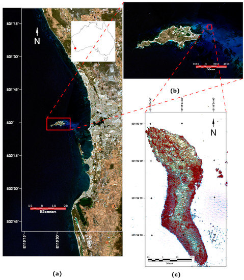
Figure 1.
(a) The City of Perth, Western Australia, the study area lies approximately 20 km west of the city. Inset shows the location in Australia. (b) Rottnest Island, with the survey area near Kingston Reef the red rectangle to the right. (c) Close-up of aerial photograph of Kingston Reef (0.2 m GSD).
Section 2.1 and Section 2.2 provide the technical details of the 3DAD SL2 LiDAR and Kongsberg EM2040c Multibeam Echosounder (MBES) systems, which were co-located on a pole with the iXblue Remotely Operated underwater Vehicle Inertial Navigation System (ROVINS) unit [25] to increase positional accuracy. Additionally, global position values were provided to the ROVINS by a CNAV 3050 GNSS, [26].
The MBES transducer, the SL2, and the ROVINS INS were mounted compactly and rigidly together, to maximise the consistency of the two data streams (see Figure 2). This allowed the relative placement of the sensors to be very accurately determined, and the close placement of the components ensured that these placements were rigid and unchanging throughout the survey.
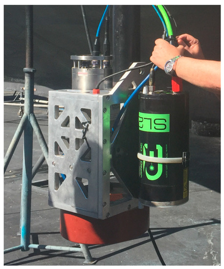
Figure 2.
View of the mounting system showing the 3DAD SL2 unit, the ROVINS, and the sonar transducer.
The shake-down and patch test were performed over a pipeline located off the coast of Perth, near Marmion Marine Park. Patch testing [27], the purpose of which is to determine the residual misalignment between the EM2040c and ROVINS reference frames, showed that the colocation of the sensors on a specifically machined high-precision sonar mount would provide bathymetric data of high quality. Calculated values for pitch, roll, and yaw between the reference frames yielded zero corrections.
2.1. Subsea LiDAR
The 3D at depth Subsea LiDAR 2 (SL2) sensor [28] used to perform the Kingston Reef survey is a time-of-flight range finding laser system. It has a stated range of 2 to 45 m (dependent on turbidity), with a range accuracy of ±4 mm over this range. In stationary mode, the “frame” of the sensor can capture a window of 30 × 30 degrees, and the whole sensor can rotate 340 degrees. A full frame of data consists of up to 1450 × 1450 points, although fewer points can be captured more rapidly. The laser-beam divergence is approximately 0.02 × 0.02 degrees, which means that the beams will overlap if the window is reduced. At a nominal 10 m water depth the diameter of the area illuminated by the laser beam is approximately 3.5 mm.
To use the SL2 to capture LiDAR from a moving platform, a single row of the frame is chosen and repeatedly scanned, with the forward motion of the vessel providing the second degree of freedom of the swath. For the data analysed here, the scanline pointing forward at 15 degrees was chosen, and the number of points sampled along this line was 296. To scan a single line of 296 points took approximately 8 ms.
Ideally, a map of the water turbidity would be consulted to ensure that the SL2 is able to function through the full range of the study area, but this was unavailable at the time of the study. The Secchi depth plays an important role in determining the useful range of this instrument, however, on the day of the survey, qualitative observations from the vessel ascertained that the water was remarkably clear, and the range of depths (8–12 m) proved to be well within the capabilities of the LiDAR system.
2.2. Multibeam Echosounder
Multibeam echosounder data were acquired using a Kongsberg EM2040c [29], operated at a constant frequency of 300 kHz with a 1.25 × 1.25-degree beam width. The EM2040c was operated in a single-head configuration, to permit colocation with the LiDAR system and ensure downward-facing orientation (see Figure 2). Positioning and motion compensation were provided by a ROVINS inertial navigation system also mounted to the pole. The EM2040c generates 400 sonar beams per ping in a fan-shaped array, thus resolution of the system varies with water depth. At a nominal 10 m water depth, the diameter of the area insonified by the multibeam is approximately 218 mm. The quoted raw range resolution of the EM2040c is 20.5 mm (27 µs pulse), with an accuracy within 10 mm.
2.3. Aerial Photography
For reference and bench-marking purposes, aerial photography was available over the Kingston Reef site. The aerial photography was captured as part of the Urban Monitor Program to acquire annual imagery over Perth and its surrounding environs [30]. The imagery is 20 cm resolution. The aerial photographs were taken with a Vexcel Ultracam [31], in January of 2016 as part of the flyovers of Rottnest Island. Figure 1c shows the aerial photography used for this study. The photography was deglinted using the method of Hedley et al. [32].
2.4. Underwater Photography
Ground truth data consist of two transects over the area with a towed video camera system, [33]. The transects were acquired by CSIRO in March 2014, but, as this is a protected marine park, the environment there has changed very little over this time.
The towed camera housing was equipped with an Ultra-Short Base Line (USBL) device to enable it to be accurately located relative to the GNSS on board the vessel. The towed video housing uses a Bosch LTC0630 camera [34]. Examples of the different habitats photographed in the area are shown in Figure 3.
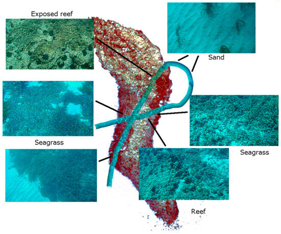
Figure 3.
Showing the principal habitats identified in the survey region.
By using the direction of travel of the camera and assuming a downward-pointing aspect, the individual frames of the video can be approximately geo-registered to aid in the identification of seafloor cover types. The geo-registration was used to roughly mosaic the video frames, so that a broad overview of the locations of habitat types could be formed. The mosaics can be laid over the other data using image processing software, such as Earth Resource (ER) Mapper [35]. The geo-registered mosaics were used to identify habitats in the aerial imagery. In Figure 3, seafloor covers are identified and marked on the aerial photograph, with the mosaicked video frames overlaid.
3. Technical Attributes of the LiDAR and MBES Data
The LiDAR data were delivered by 3D at Depth as geo-registered text files containing both depth and uncalibrated returned intensity. Ideally, to best calculate and assess the LiDAR reflectivity, full waveform data should be examined. That was not possible for the current survey, however both returned laser intensity and depth information for this dataset were provided by 3DAD.
The MBES data were processed through CSIRO’s standard processing stream. The MBES raw slant ranges were reduced to geo-registered depth measurements using the same postprocessed (NavLab; [36]) attitude and navigation that was applied to the geo-registered LIDAR. Raw slant ranges were corrected for sound velocity. The postprocessed ellipsoid height data were reduced to the Australian Height Datum (AHD) by applying geoid ellipsoid separation values from the AUSGeoid09 grid file available form Geoscience Australia [37]. These heights were further reduced from the reference point to the waterline of the vessel. This vertical and horizontal information was used to produce geo-registered point data.
The backscatter data were processed using the method of Kloser and Keith [38], which standardises the multibeam backscatter data, correcting for incidence angle, differing responses due to salinity and temperature and differences in insonified area due to sloping ground. In Figure 4, rasterised versions of the main survey area are shown, with LiDAR depth, LiDAR intensity, MBES depth, and MBES backscatter all displayed in order to show the extent and qualitative characteristics of the data.
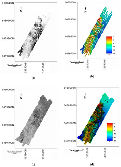
Figure 4.
(a) Light Detection and Ranging (LiDAR) intensity, (b) LiDAR bathymetry, (c) multibeam backscatter, and (d) multibeam bathymetry. Note that the LiDAR intensity and multibeam echosounder (MBES) are relative values so unscaled. All images are in SUTM50 projection.
In addition to the main dataset (KRX_Main), two additional datasets were also captured: the KRX_Lines dataset and the KRX_Star dataset, acquired to test SLAM on the data. Figure 5 shows these supplementary LiDAR datasets.
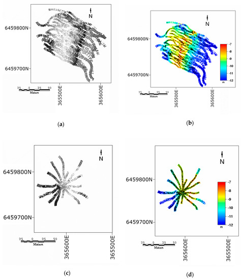
Figure 5.
(a) KRX Lines intensity, (b) KRX Lines bathymetry, (c) KRX Star intensity, and (d) KRX Star bathymetry. Note that the LiDAR intensity relative values are unscaled. All images in SUTM50 projection.
Below we present an analysis and results comparing the technical qualities of the LiDAR and MBES data. We note that this is an experimental setup, and that LiDAR has not previously been collected from a moving vessel in this fashion. It is likely that some of the observed deficiencies in the LiDAR data will be rectified in future surveys of this type. The observations presented below will enhance this process.
3.1. Comparison of LiDAR and MBES Resolution
In this subsection we compare the horizontal and vertical resolution of the LiDAR and MBES data. As EM2040c MBES is an established technology for bathymetric measurements and meets International Hydrographic Organisation (IHO) standards for hydrography, such as IHO S-44 [39]; this was considered to be the benchmark for both vertical and horizontal accuracy. To capture the variance of the two datasets, we took the standard deviation of a small patch of sand in the north of the main survey using data binned at 0.1 m. The depth of the sand patch is between 10 and 10.5 m. We found that the SD of the LiDAR and sonar data were 0.089 m for the sonar and 0.119 m for the LiDAR over this patch, indicating that the datasets have similar variance.
3.1.1. Horizontal Resolution and Accuracy
Since the points do not fit directly onto a raster grid, the horizontal resolution was measured by taking the mean distance between the scan lines and the mean distance between the points within a scanline to produce an average cross-track and along-track resolution, summarized in Table 1.

Table 1.
Mean spacing to 8 nearest neighbours for each dataset.
The LiDAR point spacing is closer across-track than the point spacing of the sonar but is approximately double the sonar in the along-track direction. This suggests that a higher scanning frequency should be employed on the lidar to bring the cross-track and along-track resolutions into closer agreement. Also note that the point spacing is not directly representative of the devices’ resolutions, since the footprint of the sensor pings are also very different.
Obtaining a qualitative gauge of the relative accuracy of the two data sources required a consistent horizontal spacing between the two. This was achieved by amalgamating the datasets to a common grid with 0.10 m spacing by taking the mean of all datapoints that fall into a particular grid. A 0.10 m spacing was chosen, as this approximately matched the insonified footprint of the sonar and enabled almost every pixel to contain a point sample from each dataset, thus minimising the need for interpolation. To assess the relative (rather than absolute) horizontal positioning accuracy of the two datasets, a set of ground control points were selected. The ground control points are selected where easily identified features are present, such as highly contrasting edges between sand and reef. To account for human errors in the selection of points, 15 points were chosen, so that the errors are averaged over many selections. Figure 6a,b show the 15 points superimposed over the LiDAR and multibeam depths, respectively.
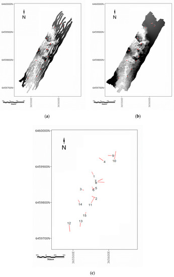
Figure 6.
15 matching control points are manually selected. (a) LiDAR and (b) MBES. (c) Displacement between multibeam and LiDAR control points exaggerated by a factor of 100. Coordinates in SUTM50.
The difference between the matching control points on each dataset are then calculated. In Figure 6c a quiver plot shows the direction of the difference between the LiDAR and MBES control points. The directions are exaggerated by a factor of 100 to enhance the display. The root-mean-square (RMS) of the lengths is approximately 0.116 m, which is less than the insonified footprint of the sonar. This, along with the fact that there is no systematic pattern in the directions of the residuals, indicates that there is no significant difference between the geolocation of these two datasets.
3.1.2. Vertical Comparison
Plots were then produced of LiDAR depth vs multibeam depth (Figure 7a) and the difference between the MBES and LiDAR depth ((Figure 7b). The median absolute difference between the lidar depth and the multibeam depth is 0.03 m, which is about double the quoted raw range resolution of the sonar.
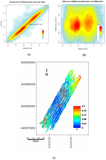
Figure 7.
(a) Plot of MBES depths verses LiDAR depths. (b) Difference between LiDAR depths and MBES depths. (c) Absolute difference in depth between MBES depths and LiDAR depths (SUTM50).
Figure 7c shows a map of the absolute difference in depth between the multibeam and the LiDAR. Although the LiDAR was amalgamated up to 0.1 m pixels, the detailed structure visible on the map reveals that the LiDAR is picking up more features compared to the MBES. This is because the footprint of the sonar beam is larger than the distance between beam centres. The system misses some details, because its footprint spans gaps in the reef, which the LiDAR––even with pixels amalgamated––can resolve.
3.2. Analysis of LiDAR Intensity
For habitat mapping and, potentially, for SLAM tasks, LiDAR reflectivity [40] provides an additional source of information. We differentiate here between LiDAR intensity, as provided by 3DAD, which is the strength of the returned signal and reflectivity, is a property of the seafloor, and––in simple terms––is the ratio of reflected to incident light intensity, from the surface in the absence of other effects. In an underwater environment it is challenging to calculate seamless LiDAR reflectivity, because the light beam diverges as it travels on its journey, and the water column attenuates and scatters the signal exponentially with distance.
3.2.1. LiDAR Intensity Saturation
In the geo-registered intensity data from this survey, there were many pixels that were saturated to their maximum value of 2047. 3DAD also supplied range–angle–angle (.raa) files separately, which consisted of point-cloud data (the range and pointing angles of the laser), along with a column indicating whether the point is saturated. These data contained a greater range of reflectivity values than the registered product, and we noted that the pixels that are flagged as “saturated” still have a changing reflectance value in the .raa files, possibly the result of a gamma function applied to the high numbers.
The saturated pixels are predominantly bright sandy areas of the image, including sandy pockets on the raised reef bed, and extensive sandy, low-lying areas. For the KRX_Main dataset, approximately 12% of the pixels were saturated (Figure 8a), which is to say that 12% of the pixels could not be binned without including a saturated point. All the remaining pixels had no saturated pixels, or the saturated pixels were excluded during binning. The saturated values indicate that the detector-gain settings were probably set too high for the clear water conditions and the relatively low-range imaging that was performed for this survey.
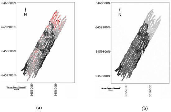
Figure 8.
(a) Red pixels are flagged as saturated. (b) LiDAR reflectivity corrected for dispersion and water column attenuation (SUTM50).
3.2.2. Water Column Attenuation and Beam Spreading
The LiDAR intensity provided by 3DAD has a clear dependence on the sensor–target distance, as illustrated in Figure 9a. The raw intensity image shows that areas in the deep water appear darker than their true reflectivity. This means that substrata that have similar reflectivity appear different, which will confound automated classification methods. In the case of Kingston Reef, the rocky reef is a prominent feature above the deeper sandy areas. Even though this macroalgae-covered reef is darker than the surrounding areas, the raw intensity shows that it is relatively bright, due to its proximity to the sensor.
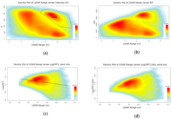
Figure 9.
Density plots of (a) provided intensity (P) vs LiDAR range (sand pixels enclosed in polygon), (b) vs LiDAR range, (c) vs LiDAR depth for sand pixels only (with fitted line), and (d) vs LiDAR range.
According to Philips and Koerber [41], the received power of the LiDAR detector is given by:
where:
- n is the refractive index of the water,
- k is the effective attenuation coefficient for the laser light through the water column,
- D is the sensor–target distance,
- A is the area of the detector,
- is the target substrate reflectance (divided by steradians when assuming a Lambertian target),
- is the power of the transmitted pulse.
Equation (1) is a simplification of the pulsed LiDAR equation from [41]. It has been simplified by removing the loss at the air–water interface (since the whole mechanism is underwater) and removing the time dependence; we are considering the pulse at the instant it is received.
We are, therefore, ignoring time-based effects, such as pulse smearing for the purpose of this analysis. The goal of the following is to estimate the reflectivity of the substrate, , uncorrupted by other effects, if possible. We assume that the provided “intensity” is a scaled version of in Equation (1). To remove the effect of the spreading LiDAR beam over distance (i.e., dispersion), the intensity data are multiplied by the square of the distance:
The effect of this is shown in Figure 9b, where all of the saturated pixels have been excluded from the analysis, and we work with LiDAR ranges from the .raa file, not depths. Note that most of the range-based effects have now been removed from the LiDAR intensity.
Taking logs of Equation (2) gives:
There are two broadly divisible populations of points: the reef (i.e., non-sand), sitting between 8 and 10 m depth as a raised plateau, and sand, sitting mostly below 10 m of depth. To normalise for attenuation effects by fitting to Equation (3), it is necessary to identify a population of pixels that each have similar target reflectance and then make the assumption that is a constant for that population. This allows the fitting of a linear equation with , , and .
We assume that the sand represents a population of roughly equal substrate reflectance. To determine the effective attenuation coefficient, a robust line is fitted to the data enclosed by the polygon in (Figure 9a), which is identified as the sand population. Figure 9c shows a density plot of against the sensor–target distance for the sand pixels only, with the saturated pixel values removed. It was necessary to subtract the minimum value from the reflectance to ensure that every number was positive, as the supplied reflectance data were arbitrarily scaled.
In the log space, the slope of this line is the coefficient . In fitting the robust line to the sand pixels, we observed a small r-squared value of 0.03, partly because the sand is not a pure colour, but mainly because the effect of water column attenuation in the clear water was quite low compared to the dispersion effect.
To remove the effect of attenuation, this slope is multiplied by depth and subtracted from the log transformed data, which is subsequently re-exponentiated to recover the original scale. The outcome is a constant multiple of with the effects of attenuation through the water column removed, as shown in Figure 8b. Note that we derived and applied the correction to the non-saturated pixels and then filled the holes with nearest neighbour interpolation. Observe that the reef and sand are far more uniformly coloured, which is consistent with them being similar materials.
4. SLAM
In the field of robotics, simultaneous localisation and mapping (SLAM) is the computational problem in which a map of an unknown environment is created based on a range information provided by a sensor (e.g., LiDAR or sonar) on a moving agent and, at the same time, the map is used to improve the localization of the agent. There are many challenges to employing SLAM in underwater environments with an AUV [16,42]. Note that the present paper is devoted to an exploration and comparison of underwater SLAM using LiDAR and sonar technology, and we make no claim of using or improving the most up-to-date SLAM techniques.
The SLAM algorithm employed here [43,44] was originally designed to work with accurate and dense range data provided by LiDAR sensors in air, using an industrial grade Inertial Measurement Unit (IMU) to provide pose estimates. Over the years, it has successfully been tested and evaluated using different modalities of range sensors, including sonars and multiple grades of inertial systems.
The algorithm works by optimizing over a sliding window of surface elements commonly known as surfels. These are features extracted directly from the point cloud. For each new iteration, the algorithm projects all the new range data into the global frame, according to a motion prior-generated from Inertial Measurement Unit (IMU) and/or basic pose estimates from external motion sensors. Then, the point cloud is split up into cubic bins called voxels. Voxels are built with spatial and temporal constraints such that a new surfel is generated for each new 3D scan of the same area. Surfels with a similar position and orientation but different time of observation are matched with a k-Nearest Neighbours (k-NN) search in a correspondence step.
Once the matching is finished, the correspondences are used to build constraints for the optimization step. The optimization procedure calculates corrections of the trajectory estimation in order to minimize the distance of two similar surfels along their mean normal. Deviations from the IMU/INS measurements are penalized to ensure smoothness of the trajectory. Finally, continuity with the previous trajectory outside of the window is enforced through initial condition constraints. Matched constraints are formed and interpolated for the discrete optimization problem. The optimization problem is solved with iterative reweighted least squares estimator. To minimize drift, the algorithm stores a set of past surfel views as fixed views, which contain surfels that were observed during a defined time span out of the window. New fixed views are stored whenever significant translational or rotational movement occurred since the last fixed view.
For the case examined here, at any given time, , the sensor (LiDAR or sonar) has a position, and an orientation, , which combine to make the six parameters of the sensor’s trajectory. For a given range measurement, (from either the LiDAR or the sonar), the trajectory implies a projection of that range measurement to a point in 3D space. Any inaccuracy in the trajectory will produce an error in the projected 3D point.
To estimate the trajectory of the sensor, the trajectory measured by the INS and GNSS is added to the offsets between the sensor and those devices. The set of six offsets between the sensor and INS/GNSS centre are called the extrinsic parameters of the system (or just “the extrinsics”). The trajectory measured by the INS/GNSS plus the (estimated or measured) extrinsics define the nominal trajectory, which is the baseline and starting estimate for further refinement. In general, SLAM algorithms provide a method to improve the nominal trajectory by matching revisited features in the projected points. If the same feature, projected from different parts of the trajectory, does not lie at the same 3D position, it implies an error in the trajectory.
There are two possible causes of error in the sensor trajectory, the first is an error in the extrinsics, or relative positions and orientations of the sensors compared to the GNSS and INS. Fixing an error in the extrinsics involves estimating a correction for the positions and orientations, , and applying it for every time . The result of applying this correction is called the calibrated trajectory, and the resulting 3D projection of the ranges is the calibrated projection.
The second cause of error is due to the INS and GNSS inaccurately estimating the trajectory; these errors are caused by an accumulated drift over time. To fix this, a different adjustment to every point on the trajectory is required; this is the output of the SLAM algorithm. The trajectory adjusted this way is called the SLAM trajectory.
To evaluate the performance of the SLAM trajectory compared to the nominal and calibrated trajectories, we collected a 16-point star dataset by executing transects up to 100 m with the objective of maximizing both the MBES and LiDAR data overlap. The SLAM algorithm was used in two different ways: firstly, it was used to get a better estimation of the extrinsics, the six offsets between the INS/GNSS, and the relevant sensor (multibeam and underwater LiDAR); and, secondly, it was applied to the dataset to get an improved trajectory estimation using the corrected extrinsics.
4.1. Using Subsea LiDAR
Figure 10a shows an overview of the underwater LIDAR dataset, KRX-Star, collected during the eight transects coloured according to the depth. It shows in detail a 16 × 11 m central section of the star where most of the overlap takes place. Only the raw trajectory is shown, since they all look very similar due to the accuracy of the GNSS/INS instruments.
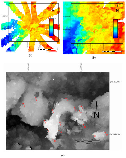
Figure 10.
Underwater 16-point star dataset with the raw trajectory projection for (a) LiDAR and (b) MBES. (c) Control points used to assess the effectiveness of simultaneous localisation and mapping (SLAM). Background is nominal LiDAR depth, shown in grey scale to highlight the control points (SUTM50).
4.2. Multibeam Echosounder
Figure 10b shows an overview of the MBES data collected during the eight transects, coloured according to the depth. The central section with most of the overlap is approximately 64 × 37 m. It is not readily apparent from the imagery, but close inspection shows that features are better defined on the calibrated trajectory compared to the raw one, although the MBES was not accurately modelled to take into account the particularities of the sensor beams’ footprints. The projected data appear identical when using the calibrated or SLAM trajectories.
4.3. Evaluating the Performance of SLAM for LiDAR and Sonar Devices
We take two different approaches to evaluate the performance of the SLAM algorithms on the LiDAR and sonar datasets, a direct method using manually selected ground control points (GCP’s) and a consistency-based errors metric from the current literature.
4.3.1. GCP Approach
To evaluate the performance of the SLAM algorithm on the LiDAR and sonar datasets, the output point clouds were again rasterised onto a 0.1 m grid. A set of 15 high-contrast control points were chosen manually in the central overlapping region (see Figure 10c) and a 11 × 11 neighbourhood window of each control point was extracted to form exemplars using the nominal point cloud projections.
For each of the nominal, calibrated, and SLAM projection results, an automated search was performed to find the location in each arm of the star that best matched the exemplars. The matching was determined using the normalised cross-correlation function [45] over the window. After matching the points at the pixel level, subpixel matching was performed using bilinear interpolation to achieve the best estimates possible for the control point locations in each of the strips and for each dataset. To ensure that well-matched points were used, only matches that had a normalised cross-correlation score of 0.9 or more were considered for the remainder of the analysis.
To assess how well the control points agree within a given dataset, we calculated the standard deviation (SD) for each of the 15 control points with more than two matches from different arms of the star. Table 2 summarises the results for the LiDAR and sonar datasets.
Table 2.
Consistency of LiDAR control points expressed as root-mean-square (RMS) distance from the mean of each set of matched control points.
For the LiDAR dataset, the differences in the nominal projections of control points have mean SD of 0.065 m. By using SLAM to improve the extrinsics calibration to get a better estimation of the INS and LiDAR relative poses, the mean SD improves to 0.058 m. The projection from the SLAM trajectory with the corrected extrinsics lowers the mean SD to 0.036 m, which is less than the along-track spacing of the dataset (0.063 m).
For the sonar dataset, the mean SD of control points for the nominal projection, 0.124 m, is improved by the extrinsics calibration and SLAM trajectories to 0.093 m and 0.079 m, respectively. However, since the MBES insonified area is of a similar magnitude, it is not clear that the SLAM technique provides a significant improvement beyond the extrinsics calibration using this evaluation technique (as both improvements would be considered “subpixel”). Additional data collection in a controlled environment that contains grid markers and objects of known size would be required to explore whether the algorithm improves the nominal sensor specifications.
4.3.2. Consistency Metric Approach
To further illuminate the consistency of the various versions of the sonar and LiDAR datasets in their nominal, calibrated, and SLAM’d versions, we implemented the method of Roman and Singh [46]. This method is a point-based error metric that can be used to evaluate self-consistency where map regions have been imaged multiple times.
In our case, the metric can be calculated for every pixel where the pixel and its neighbours have been scanned by more than one revisit of the scanner. Each revisit of the scanner creates a distinct cloud of points, called a surface patch.
The method proceeds by determining the set-wise distance between each point and the nearest points on any other overlapping surface patch. The metric is then given for each bin (in our case, pixels) by largest set-wise distance amongst the entire set of maps, contributing points to that pixel and its neighbours. According to [46], the method is less effected by the choice of bin size than other consistency measures. Figure 11 shows the results of implementing the Roman and Singh method. Table 3 summarises the results. The consistency-based error metric shows trends that agree with the previous method of evaluating the datasets, i.e., that the nominal, calibrated, and SLAM’d datasets are increasingly self-consistent, and that the SLAM does not provide a lot of improvement in the sonar consistency.
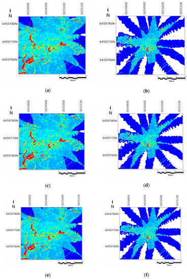
Figure 11.
(a) Nominal sonar. (b) Nominal LiDAR. (c) Calibrated sonar. (d) Calibrated LiDAR. (e) SLAM’d sonar. (f) SLAM’d LiDAR.
Table 3.
Statistics for the Roman and Singh consistency-based error metric for the 3 LiDAR datasets.
5. Benthic Habitat Mapping
To demonstrate the value of incorporating both LiDAR reflectivity and multibeam backscatter into a benthic habitat classification, we have provided a classification of the combined LiDAR and MBBS data. The classification is performed by selecting training sites according to the available ground truth (Figure 3). The LiDAR reflectivity is calibrated according to the procedure in Section 3.2.2 (note that this has changed the scale of the LiDAR Reflectivity). Saturated points have been removed and filled in with nearest neighbour interpolation.
The ground truth data lead to the choice of four different substrata for classification purposes, with the following qualities:
- Sand: Consists of bright material that is soft, with little texture on the aerial image. This has high LiDAR reflectivity and low backscatter.
- Seagrass: This grows on the sand, so tends to also be a soft substrate, however it is much darker. Has low backscatter and low reflectance compared to sand.
- Exposed reef/sand veneer over reef: A hard material that is bright. This will have a high backscatter and a high reflectivity.
- Reef with macro algae: This is relatively dark and hard. It, therefore, has a low reflectivity (compared to sand) but a high backscatter.
The training sites selected consist of rectangles of various sizes, depending on the benthic habitat that is being trained on. Figure 12a shows a plot of the means of the 29 training sites that were selected. In Table 4 the total number of training sites and pixels for each cover type are shown.
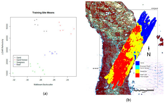
Figure 12.
(a) Classification scheme for combined LiDAR reflectivity and multibeam backscatter data. (b) A classified map produced with LiDAR reflectivity and multibeam backscatter (SUTM50).
Table 4.
The number sites and pixels for each training class.
To perform the classification, a random sample of 100 pixels from each of the training data were selected to train a maximum likelihood classifier (MLC; [47]), with an additional 50 pixels chosen from the remaining ground truth data for validation. The classifier was then used to train the remaining pixels in the image, while the validation data were used to perform estimates of the accuracy (see Table 5). We performed three classifications, one using just the LiDAR reflectivity, a second with only the MBBS, and a third with both.
Table 5.
Confusion matrix for the maximum likelihood classifier.
After the MLC was performed, a majority filter of size 5 × 5 pixels was passed over the classified image to smooth out some of the speckle and fill the gaps in between swaths. Figure 12b shows the results of the classification using both the reflectivity and the backscatter. This appears to be a sensible result, as it is consistent with the ground truth and additional data that are available in this study.
The plot in Figure 12a suggests that the Sand and Seagrass classes are difficult to resolve without the inclusion of LiDAR reflectivity, since they have very similar hardness. On the other hand, the Sand and Sand Veneer/Exposed Reef classes have very similar reflectivity, suggesting that the MBBS plays an important role in discriminating between them. These hypotheses are backed up by the confusion matrices for the classification performed with only backscatter and with only LiDAR, shown in the bottom rows of Table 5. The combination of LiDAR reflectivity and MBBS allows separation between classes that would not have been possible with either one alone.
6. Discussion and Future Work
We analysed and compared the specifications for simultaneously acquired ship-mounted LiDAR and multibeam data. To our knowledge, no surveys of this type have been previously conducted; although both systems have been simultaneously mounted on an ROV [14], a detailed comparison of the data sources has not been published.
In the context of underwater SLAM collecting LiDAR, multibeam, and INS data with the same spatial and temporal constraints, provides an opportunity to examine the two technologies under the same conditions, ensuring a fair comparison of the results.
The subsea LiDAR data have superior spatial resolution to the sonar, the LiDAR footprint is 25 times smaller, which allowed greater detail to be resolved on the seafloor. In the case of MBES, increasing the point density will not increase the resolution of the data, because the footprints of the beams overlap, so there is blurring between neighbouring point samples.
The horizontal agreement between the LiDAR and multibeam data is quite good, but the registration was not completely independent since the multibeam data were provided to 3DAD before delivery of the LiDAR data.
There was a fair proportion of saturated pixels in the bright sandy regions, which lead to some data loss. This could be resolved by varying the gain of the LiDAR according to the reflectivity of the target, using either a physical or empirical model. A variable detector gain (whose value is recorded in the metadata) and a heuristic for setting it would allow for a greater range of reflectivity values to be recorded without saturation. Since this data collection was performed, the 3D at Depth LiDAR now has a “Real Time Viewer” that allows the operator to identify saturation while collecting the data and, therefore, make corrections in real time.
SLAM has been successfully evaluated on both the LiDAR and multibeam datasets. In both cases it has improved the accuracy of the relative position of the INS and each sensor head, increasing the quality of the dataset when projected from the trajectory. For the case of MBES sonar, the results show that SLAM does not significantly improve the trajectory estimation on a high-end GNSS and INS system, which is typically used as a ground truth for mapping algorithms. However, it would provide improved accuracy when the navigation system is not available, such as on ROVs or AUVs. For the LiDAR data, the SLAM did provide a significant improvement, regardless of the availability of the GNSS; further analysis is required to identify why the results for LiDAR and sonar are different.
As future work on this topic we will perform multimodal SLAM using both the multibeam LiDAR readings, which requires accurate sensor modelling of the multibeam sonar to account for the energy distribution of each of the beams’ footprints.
Airborne LiDAR and sonar have been analysed and compared for habitat mapping purposes [22], but it was not simultaneously acquired from the same platform with a shared INS as here. In [48], the authors explore the use of optical (IKONOS) and dual frequency side-scan sonar for mapping reef environments. They found a significant misclassification between seagrass and algae-covered habitats when only using the optical data. When using the acoustic data, their seagrass had the poorest discrimination of all the classes, being confused with sandy habitats with some rubble. There was a significant improvement in mapping all classes when both acoustic and optical data were used.
It has been demonstrated that the LiDAR reflectivity and MBBS are complementary data sources for habitat mapping, allowing for more classes to be mapped than either one alone. This is because the acoustic reflectivity (i.e., MBES backscatter) and green laser reflectivity are independent measurements that can be used to characterise seafloor substrata. Future work with more ground truth will allow for further quantitative analysis to confirm this.
A disadvantage of current time-of-flight subsea LiDAR systems is that they have been developed for deep-water metrology applications for industries that build and maintain subsea infrastructure [21]. Whilst these systems can be mounted on moving platforms, they have primarily been designed for use in a fixed station setting to monitor large survey areas, utilising reference locations to be systematically moved to different fixed points around the survey area. The design priorities are for very high accuracy and range, along with the ability to withstand great depths and hostile deep-water environments. This increases their cost considerably, while not necessarily being an advantage for shallow water benthic habitat mapping missions, where centimetre accuracy is likely to be sufficient. A systems-engineering approach to integration of the LiDAR onto a moving platform is likely to provide superior results, given that the SL2 is designed to capture stationary frames. We have shown that a light-weight LiDAR system with the ability to be rapidly deployed from a moving platform may enhance the speed and accuracy of benthic habitat mapping and enable improved navigation in the absence of GNSS or other absolute localisation techniques.
In future work, we will be developing experimental green laser setups to provide further insights into the pulse detection and reflectivity calculations from subsea LiDAR systems. An understanding of the full waveform, rather than just the processed outputs from a commercial system, will provide the flexibility needed to set pulse detections based on brightness and to adjust the detector dynamics to avoid saturation, enabling superior habitat mapping and robot navigation. Ultimately, a purpose-built, low-cost, shallow-water system will allow more flexibility to experiment on AUV systems in coral-reef environments.
Author Contributions
Conceptualization, S.C., T.J.M. and A.M.; methodology, S.C., E.H. and T.J.M.; software, S.C.; validation, S.C. and C.E.; investigation, M.B., A.F., S.E. and G.C.; data curation, M.B.; writing—original draft preparation, S.C.; writing—review and editing, S.C., C.E., T.J.M. and S.E.; All authors have read and agreed to the published version of the manuscript.
Funding
This research received no external funding.
Acknowledgments
Adam Lowry for helping to conceive the survey, helping to install the SL2, and operating the SL2 on the voyage. Steve Harris and Pat Fournier at Neptune Marine Services for lending us a data transmission cable for the ROVINS at short notice. Dave Donohue from iXBlue for lending us the Delph INS dongle for processing the LiDAR data. Ryan Crossing for technical support on the vessel. Engineering Technical Services (ETS) at CSIRO Hobart for manufacture of test equipment used to mount instruments. This work was funded by the CSIRO’s Active Integrated Matter (AIM) Future Science Platform.
Conflicts of Interest
The authors declare no conflict of interest.
References
- Kritzer, J.; DeLucia, M.-B.; Greene, E.; Shumway, C.; Topolski, M.; Thomas-Blate, J.; Chiarella, L.; Davy, K.; Smith, K. The importance of benthic habitats for coastal fisheries. BioScience 2016, 66, 274–284. [Google Scholar] [CrossRef]
- Piacenza, S.E.; Barne, A.K.; Benkwit, C.E.; Boersma, K.S.; Cerny-Chipman, E.B.; Ingeman, K.E.; Kindinger, T.L.; Lee, J.D.; Lindsley, A.J.; Reimer, J.N.; et al. Patterns and Variation in Benthic Biodiversity in a Large Marine Ecosystem. PLoS ONE 2015, 10, e0135135. [Google Scholar] [CrossRef] [PubMed]
- Chong-Seng, K.; Mannering, T.; Pratchett, M.; Bellwood, D.; Graham, N. The influence of coral reef benthic condition on associated fish assemblages. PLoS ONE 2012, 7, e42167. [Google Scholar] [CrossRef] [PubMed]
- Komyakova, V.; Jones, G.; Munday, P. Strong effects of coral species on the diversity and structure of reef fish communities: A multi-scale analysis. PLoS ONE 2018, 13, e0202206. [Google Scholar] [CrossRef] [PubMed]
- Ostrander, G.; Armstrong, K.; Knobbe, E.; Gerace, D.; Scully, E. Rapid transition in the structure of a coral reef community: The effects of coral bleaching and physical disturbance. Proc. Natl. Acad. Sci. USA 2000, 97, 5297–5302. [Google Scholar] [CrossRef] [PubMed]
- Mellin, C.S.; Anthony, K.; Brown, S.; Caley, M.; Johns, K.; Osborne, K.; Puotinen, M.; Thompson, A.; Wolff, N.; Fordham, D.; et al. Spatial resilience of the Great Barrier Reef under cumulative disturbance impacts. Glob. Chang. Biol. 2019, 25, 2431–2445. [Google Scholar] [CrossRef] [PubMed]
- Bridge, T.; Beaman, R.; Done, T.; Webster, J. Predicting the location and spatial extent of submerged coral reef habitat in the Great Barrier Reef World Heritage Area, Australia. PLoS ONE 2012, 7, e48203. [Google Scholar] [CrossRef]
- Marouchos, A.; Dunbabin, M.; Muir, B.; Babcock, R. A shallow water AUV for benthic and water column observations. In Proceedings of the IEEE Oceans 2015—Genoa, Genoa, Italy, 18–21 May 2015. [Google Scholar]
- Day, J. The need and practice of monitoring, evaluating and adapting marine planning and management—Lessons from the Great Barrier Reef. Mar. Policy 2008, 32, 823–831. [Google Scholar] [CrossRef]
- Zieger, S.; Stieglitz, T.; Kininmonth, S. Mapping reef features from multibeam sonar data using multiscale morphometric analysis. Mar. Geol. 2009, 264, 209–217. [Google Scholar] [CrossRef]
- Kayal, M.; Vercelloni, J.; de Loma, T.L.; Bosserelle, P.; Chancerelle, Y.; Geoffroy, S. Predator crown-of-thorns starfish (acanthaster planci) outbreak, mass mortality of corals, and cascading effects on reef fish and benthic communities. PLoS ONE 2012, 7, e47363. [Google Scholar] [CrossRef]
- Marine Technology. 3D at Depth Completes 300 Offshore LiDAR Metrologies. 2018. Available online: https://www.marinetechnologynews.com/news/depth-completes-offshore-LiDAR-556673 (accessed on 3 April 2019).
- O’Byrne, M.; Pakrashi, V.; Schoefs, F.; Ghosh, B. A comparison of image based 3d recovery methods for underwater inspections. In Proceedings of the 7th European Workshop on Structural Health Monitoring, Nantes, France, 8–11 July 2014. [Google Scholar]
- McLeod, D.; Jacobson, J.; Hardy, M.; Embry, C. Autonomous inspection using an underwater 3d LiDAR. In Proceedings of the MTS/IEEE Oceans, San Diego, CA, USA, 23–27 September 2013. [Google Scholar]
- Turner, J.A.; Babcock, R.C.; Hovey, R.; Kendrick, G.A. AUV-based classification of benthic communities of the Ningaloo shelf and mesophotic areas. Coral Reefs 2018, 37, 763–778. [Google Scholar] [CrossRef]
- Guth, F.; Silveira, L.; Botelho, S.; Drews, P.; Ballester, P. Underwater SLAM: Challenges, state of the art algorithms and a new biologically-inspired approach. In Proceedings of the 5th IEEE RAS/EMBS International Conference on Biomedical Robotics and Biomechatronics, Sao Paulo, Brazil, 12–15 August 2014. [Google Scholar]
- Rodrgues, M.; Kormann, M.; Schuhler, C.; Tomek, P. Structured light techniques for 3D surface reconstruction in robotic tasks. In Advances in Intelligent Systems and Computing; Kacprzyk, J., Ed.; Springer: Heidelberg, Germany, 2013; pp. 805–814. [Google Scholar]
- Massot-Campos, M.; Oliver-Codina, G. Optical sensors and methods for underwater 3D reconstruction. Sensors 2015, 15, 31525–31557. [Google Scholar] [CrossRef] [PubMed]
- Chong, T.J.; Tang, X.J.; Leng, C.H.; Yogeswaran, M.; Ng, O.E.; Chong, Y.Z. Sensor technologies and simultaneous localization and mapping (SLAM). Proc. Comput. Sci. 2015, 76, 174–179. [Google Scholar] [CrossRef]
- Burguera, A.; González, Y.; Oliver, G. Sonar sensor models and their application to mobile robot localization. Sensors 2009, 9, 10217–10243. [Google Scholar] [CrossRef]
- Filisetti, A.; Marouchos, A.; Martini, A.; Martin, T.; Collings, S. Developments and applications of underwater LiDAR systems in support of marine science. In Proceedings of the OCEANS 2018 MTS/IEEE Charleston, Charleston, SC, USA, 22–25 October 2018. [Google Scholar]
- Costa, B.; Battista, T.; Pittman, S. Comparative evaluation of airborne LiDAR and ship-based multibeam sonar bathymetry and intensity for mapping coral reef ecosystems. Remote Sens. Environ. 2009, 113, 1082–1100. [Google Scholar] [CrossRef]
- Kotilainen, A.; Kaskela, A. Comparison of airborne LiDAR and shipboard acoustic data in complex shallow water environments: Filling in the white ribbon zone. Mar. Geol. 2017, 385, 250–259. [Google Scholar] [CrossRef]
- Collings, S.; Campbell, N.; Keesing, J. Quantifying the discriminatory power of remote sensing technologies for benthic habitat mapping. Int. J. Remote Sens. 2019, 40, 2717–2738. [Google Scholar] [CrossRef]
- iXblue. ROVINS Datasheet. 2014. Available online: https://www.ixblue.com/sites/default/files/datasheet_file/ixblue-ps-rovins-02-2014-web.pdf (accessed on 28 March 2019).
- Oceaneering. C-Nav3050 GNSS Reciever. 2018. Available online: https://www.oceaneering.com/datasheets/C-Nav-C-Nav3050.pdf (accessed on 5 September 2019).
- Gueriot, D.J.; Daniel, S.; Maillard, E. The patch test: A comprehensive calibration tool for multibeam echosounders. In Proceedings of the OCEANS 2000 MTS/IEEE Conference and Exhibition, (Cat. No.00CH37158), Providence, RI, USA, 11–14 September 2000. [Google Scholar]
- 3D at Depth. SL2 Product Sheet. 2019. Available online: https://www.3datdepth.com/product/sl2-LiDAR-laser (accessed on 28 March 2019).
- Kongsberg. EM2040C Multibeam Echo Sounder Data Sheet. 2014. Available online: https://www.kongsberg.com/globalassets/maritime/km-products/product-documents/369468_em2040c_product_specification.pdf (accessed on 31 October 2019).
- Caccetta, P.; Collings, S.; Devereux, A.; Hingee, K.; McFarlane, D.; Traylen, A.; Wu, X.; Zhou, Z. Monitoring land surface and cover in urban and peri-urban environments using digital aerial photography. Int. J. Digit. Earth 2016, 9, 457–475. [Google Scholar] [CrossRef]
- Vexcel. The Vexcel UltraCam Large Format Digital Aerial Camera. 2004. Available online: https://www.geoshop.hu/images/static/UltracamD_UCD_brochure.pdf (accessed on 28 March 2019).
- Hedley, J.; Harborne, A.; Mumby, P. Simple and robust removal of sun glint for mapping shallow-water benthos. Int. J. Remote Sens. 2005, 26, 2107–2112. [Google Scholar] [CrossRef]
- Underwood, M.; Sherlock, M.; Marouchos, A.; Forcey, K.; Cordell, J. A portable shallow-water optic fibre towed camera system for coastal benthic assessment. In Proceedings of the OCEANS 2018 MTS/IEEE Charleston, Charleston, SC, USA, 22–25 October 2018. [Google Scholar]
- Bosch. LTC0630 Camera Datasheet. 2013. Available online: http://resource.boschsecurity.com/documents/Data_sheet_enUS_2012582795.pdf (accessed on 31 October 2019).
- Hexagon Geospatial. ER Mapper Brochure. 2019. Available online: https://www.hexagongeospatial.com/brochure-pages/erdas-ermapper-professional-benefit-brochure (accessed on 29 May 2020).
- Gade, K. NavLab, a generic simulation and post-processing tool for navigation. Eur. J. Navig. 2004, 2, 21–59. [Google Scholar] [CrossRef]
- Geoscience Australia, “AUSGeoid09,”. 2009. Available online: https://s3-ap-southeast-2.amazonaws.com/geoid/AUSGeoid09_V1.01.gsb (accessed on 29 July 2020).
- Kloser, R.; Keith, G. Seabed multi-beam backscatter mapping of the Australian continental margin. Acoust. Aust. 2013, 41, 65–72. [Google Scholar]
- IHO. Standards for Hydrographic Surveys, 5th ed.; Special Publication No. 44; International Hydrographic Bureau: Monaco, 2008. [Google Scholar]
- Kopilevich, Y.; Feygels, V.; Tuell, G.; Surkov, A. Measurement of ocean water optical properties and seafloor reflectance with scanning hydrographic operational airborne lidar survey (SHOALS): I. Theoretical background. In Proceedings of the SPIE Conference on Optics and Photonics 2005, Remote Sensing of the Coastal Oceanic Environment, San Diego, CA, USA, 31 July–4 August 2005; Volume 5885. [Google Scholar]
- Phillips, D.M.; Koerber, B.W. A theoretical study of an airborne laser technique for determining sea water turbidity. Aust. J. Phys. 1984, 37, 75. [Google Scholar] [CrossRef]
- Barkby, S.; Williams, S.; Pizarro, O.A.J.M. A featureless approach to efficient bathymetric SLAM using distributed particle mapping. J. Field Robot. 2011, 28, 19–39. [Google Scholar] [CrossRef]
- Bosse, R.; Zlot, M. Continuous 3d scan-matching with a spinning 2D laser. In Proceedings of the International Conference on Robotics and Automation, Kobe, Japan, 12–17 May 2009. [Google Scholar]
- Bosse, M.; Zlot, R.; Flick, P. Zebedee: Design of a spring-mounted 3D range sensor with application to mobile mapping. IEEE Trans. Robot. 2012, 5, 1104–1119. [Google Scholar] [CrossRef]
- Kraus, K. Photogrammetry; Dummler: Bonn, Germany, 1997; Volume 2: Advanced Methods and Applications; Available online: https://www.worldcat.org/title/photogrammetry-vol-2-advanced-methods-and-applications/oclc/59385641 (accessed on 30 July 2020).
- Roman, C.; Singh, H. Consistency based error evaluation for deep sea bathymetric mapping with robotic vehicles. In Proceedings of the International Conference on Robotics and Automation, Orlando, FL, USA, 15–19 May 2006; IEEE: Piscataway, NJ, USA, 2006. [Google Scholar]
- Hastie, T.; Tibshirani, R.; Friedman, J. The Elements of Statistical Learning; Springer: New York, NY, USA, 2001. [Google Scholar]
- Malthus, T.; Karpouzli, E. On the Benefits of Using Both Dual Frequency Side Scan Sonar and Optical Signatures for the Discrimination of Coral Reef Benthic Communities. Advances in Sonar Technology. 2009, pp. 165–190. Available online: https://www.intechopen.com/books/advances_in_sonar_technology/on_the_benefits_of_using_both_dual_frequency_side_scan_sonar_and_optical_signatures_for_the_discrimi (accessed on 30 July 2020).
© 2020 by the authors. Licensee MDPI, Basel, Switzerland. This article is an open access article distributed under the terms and conditions of the Creative Commons Attribution (CC BY) license (http://creativecommons.org/licenses/by/4.0/).