Internal Wave Dark-Band Signatures in ALOS-PALSAR Imagery Revealed by the Standard Deviation of the Co-Polarized Phase Difference

Abstract

Analysis of synthetic aperture radar (SAR) images in L-band of short-period internal waves (IWs), and classification of their radar signatures is presented by means of a polarimetric data set from ALOS-PALSAR mission. We choose the polarimetric feature named standard deviation(std) of the co-polarized phase difference (CPD) to identify fundamental differences in SAR signatures of internal waves, and divided them into three different classes, according to their backscattered modulation depths and morphology as well as the std CPD, namely: double-signed, single-negative, and single-positive signatures, for IW normalized image transects that display, respectively, signatures in the form of bright/dark, dark, and bright bands that correspond to positive/negative, negative, or positive variations of radar backscatter. These radar power types of signatures have a counterpart in the std CPD normalized transects, and in this paper we discuss those correlations and decorrelations. We focus in the single-negative type of signature, that is dark bands on gray background, and show that the std CPD is greatly enhanced over the troughs and rear slopes of those IWs. It is suggested that such behavior is consistent with the presence of surface slicks owing to enhanced surfactant concentration. Furthermore, those single-negative SAR signatures appear at locations where and when biological productivity is enhanced. It is found that the modulation depths associated to the std CPD is higher than the one associated to the HH-polarized radar backscatter for single-negative signatures propagating in the range direction, while the reverse occurs for the other types of signatures.

1. Introduction

Internal waves (IWs) are widespread, distributed around the world’s oceans as the result of the variety of ways they can be generated (including from nonlinear disintegration of internal tides, lee waves, resonance, tidal beams, buoyant near-surface plumes, etc; see e.g., [1]). The diversity of the generation mechanisms, environmental conditions, and locations produce waves with wavelengths ranging from few tens of meters to kilometers; however, all reasonably described by some solitary wave theory. The IWs propagate in the ocean along the pycnocline, i.e., a water column portion characterized by a sharp change in density resulting, typically, from temperature and/or salinity vertical gradients. They connect large-scale tides to smaller scale turbulence and retain their form for a long time period after their generation [1].

The IWs are important for heat exchange in the vertical, as well as nutrients vertical exchange and other properties between shelf and the open ocean, playing a key role in biological primary production [2] and in the understanding of the climate system evolution. Furthermore, they have an economical importance since they can represent a risk to offshore drilling operations [1], or possibly be relevant for aquaculture activities.

Research efforts concerning IWs are often based on satellite observations since they provide insights into their generation, propagation, and dissipation mechanisms as well as render the two-dimensional horizontal structure of the IWs. Within this context, the systematic observation of IWs by means of synthetic aperture radar (SAR) is widely reported in the literature [3,4,5], as well as the variety of factors that impacts their signatures in that imagery [3,6,7]. IWs interact with the ocean surface and modify their roughness, appearing on SAR imagery typically as alternating series of quasi-periodic bright and dark linear or curvilinear bands on a gray background. The bright and dark bands result from variations in the subsurface currents associated with the IWs and their interaction with the ocean surface wind waves. These interactions produce, respectively, a convergent (rough) and divergent (smooth) surface zone [3,4]. The signatures of IWs in the form of bright/dark bands were discussed by [3] based on the weak hydrodynamic interaction and Bragg scattering theory using L-band SAR imagery. Although this theory is capable to describe quite well the IWs signatures on co-polarized SAR measurements (i.e., HH and VV channel), studies developed by [8] using copolarized C-band SAR imagery show that the contribution of non-polarized scattering caused by breaking waves is not negligible. Furthermore, their signature patterns can be affected by parameters related to the IWs themselves (mode, half-width, amplitude, and background currents) and to environmental parameters. The latter includes the wind conditions and the presence of surface films [6,9].

Considering the influence of the wind speed on the IW patterns, under low wind conditions (i.e., lower than 2 m/s) the IWs show up as predominant bright intensity variations [6]; while, under wind speeds higher than 2 m/s and along the satellite track direction (i.e., IWs propagating in the radar azimuth direction), the dark signatures are predominant [6]. For wind speed higher than 2 m/s and across track direction (i.e., range propagating IWs), the IW patterns commonly observed are both alternating bright/dark and predominant dark signatures [6].

An observer watching the ocean when winds are low (i.e., below 6–7 m/s) would soon notice that some areas of the surface appear smoother than adjacent areas. These smooth areas, called surface slicks, are often visible as long bands also identifiable from space [6,10,11] with high-resolution remote sensing techniques such as SAR. Ocean slicks are believed to be primarily composed of naturally occurring surface-active substances (surfactants) which concentrate in the form of films on the surface. Very often they occur in regions of increased biological activity such as coastal and estuarine waters, near the polar ice boundaries or near oceanic fronts. The primary source of surfactants are exudates from phytoplankton or zooplankton grazing [12,13,14]. Surfactants are concentrated in a film form in the sea surface micro-layer, the boundary layer between the ocean and the atmosphere defined as the uppermost 50–100 micrometers [14]. Surfactants can modify physical properties of the ocean by altering surface tension in response to small changes of surface area caused by the compression or dilation of the local surface as ripple waves propagate by [11,15,16]. The effect includes dampening of short gravity-capillary waves. Horizontal convergences due to current field variations at the ocean surface, such as those due to the orbital velocity of IWs, can compress the surfactant materials and form a surface-elastic film and these films can become concentrated enough to also attenuate surface waves.

The surface films interact with the internal wave currents causing changes on the IWs patterns on SAR imagery. According to [6,9] the surface film concentration is enhanced in convergence zones associated to the IWs; while it is reduced in the divergent zones. Thus, since the damping properties associated to the surface films reduce the small Bragg resonant waves resulting in a smaller percentage of radar signal to be scattered back to the radar system, the IWs patterns can be seen as dark bands, the bright bands being either absent or strongly attenuated as a result of film modulation [6].

In this paper we consider mainly L-band ALOS-PALSAR image data at small to moderate incidence angles, i.e., 22 to 25 degrees, and hence it is assumed that Bragg scattering can account, to first order, for radar signatures in these conditions [3]. Following the pioneer results revealed in [3], the radar modulation depths as well as its form (bright and dark bands that we denominate double-sign signatures in this article), do capture most of the IW signatures that have been observed in L-band SARs. However, there are many instances when the L-band signatures of IWs appear as dark bands on a gray background, as in the case of Figure 1, the usually companion bright bands being either absent or strongly attenuated. This fact is consistent with film slick effects proposed in [6] for C-band SARs, but it is also applicable to L-band (see [6] and their Figure 13). Here we discuss in some detail dark-band signatures such as those in Figure 1, which we denominate single-negative signatures, using a method known as the standard deviation of the co-polarized phase difference [17,18]. In this framework, it is well known that the SAR polarimetry provides extra benefits for a range of marine applications [17,18] and in the literature several polarimetric features measuring the departure from the almost deterministic sea surface Bragg scattering have been proposed [18].

The polarimetric feature named standard deviation (std) of the co-polarized phase difference (CPD) is related to the scattering properties of the observed scene and it is considered a measure of the complex correlation between the co-polarized channels. The latter polarimetric feature has been recognized to be very effective for surface slick observation purposes discriminating an oil slick from a weak-damping surfactant film [19]. Furthermore, the standard deviation of the CPD has been shown almost independent of the estimation window size and unbiased when low correlation of co-polarized channels applies [19,20]. It is important to highlight that the std CPD behavior is affected by incidence angle, noise equivalent sigma zero (NESZ), and meteo-marine conditions as discussed by [21,22,23].

In this paper, further insights on the effects of the surface films on the IW patterns in SAR imagery are analyzed by means of the std CPD for the first time in literature. The theoretical background is presented in Section 2. In Section 3, the study area is presented as well as the SAR data set and the ancillary information are described. The experimental results and discussion are presented in Section 4. Finally, the conclusion is shown in Section 5.

2. Theoretical Background

The complete Scattering matrix S is measured by a fully-polarimetric SAR. Taking into account the horizontal–vertical linearly polarized electric fields, S can be expressed as in [24]

$$S=\left(\begin{array}{cc}{S}_{HH}& S_{HV}\\ S_{VH}& S_{VV}\end{array}\right)$$

(1)

The scattering amplitude, i.e., each complex element of S, is expressed as

$$S_{sq}={\left|S_{sq}\right|}^{e^{j{\varphi }_{sq}}}$$

(2)

where $\left\{sq\right\}=\left\{HV\right\}$. Upon the assumption of reciprocity (i.e., the two cross-polarized terms are equal, $S_{HV}=S_{VH}$ [24]), we can write Equation (1) as

$$S=e^{j{\varphi }_{VV}}\left(\begin{array}{cc}{S}_{HH}{e}^{j{\varphi }_{CPD}}& S_{HV}{e}^{j{\varphi }_{XPD}}\\ S_{HV}{e}^{j{\varphi }_{XPD}}& S_{VV}\end{array}\right)$$

(3)

where

$${\varphi }_{CPD}=\angle S_{HH}{S}_{VV}^{*}={\varphi }_{HH}-{\varphi }_{VV}$$

(4)

and

$${\varphi }_{XPD}=\angle S_{HV}{S}_{VV}^{*}={\varphi }_{HV}-{\varphi }_{VV}$$

(5)

are, respectively, the CPD and cross-polarized phase difference, where ∠ and ${}^{*}$ stand for the phase part and complex conjugate operator, respectively. For most natural targets, the XPD probability density function (pdf) follows approximately a uniform distribution over $\left[-\pi ,\pi \right]$ [25], therefore, it contains less specific information related to the target. The analytical expression of the CPD pdf is given by [26,27]

$$p\left({\varphi }_{CPD}\right)=\frac{\left(1-{\rho }^2\right)\mathsf{\Gamma }\left(2N\right)}{2\left(N+\frac{1}{2}\right)\sqrt{\pi }\mathsf{\Gamma }\left(N\right)}{\left(\frac{1}{1-{\beta }^2}\right)}^{\frac{N+\frac{1}{2}}{2}}{L}_{N-\frac{3}{2}}^{-N-\frac{1}{2}}\left(-\beta \right)$$

(6)

where

$$\beta =\rho cos\left({\varphi }_{CPD}-{\mu }_{{\varphi }_{CPD}}\right)$$

(7)

and N is the number of looks, $\rho$ is the correlation of the co-polarized channels, $L\left(·\right)$ and $\mathsf{\Gamma }\left(·\right)$ are the first kind-Legendre and Gamma functions, respectively. Considering $0<\rho <1$, the CPD pdf resembles a Gaussian bell with mean represented by ${\mu }_{{\varphi }_{CPD}}$ and standard deviation henceforth denominated by ${\sigma }_{{\varphi }_{CPD}}$. The increasing N or $\rho$ implies that the CPD pdf becomes narrower. Thus, when $\rho$ tends to 0, the CPD pdf is uniformly distributed between $\left[-\pi ,\pi \right]$; otherwise, when $\rho$ tends to 1, the CPD pdf tends to a Dirac delta function. The ${\sigma }_{{\varphi }_{CPD}}$ is inversely proportional to $\rho$ [19,26,27].

Considering a homogeneous sea surface where the Bragg scattering applies, the cross-polarized scattering amplitudes are almost negligible, a low depolarizing effect is expected as well as a high correlation between the co-polarized channels. Thus, a low ${\sigma }_{{\varphi }_{CPD}}$ value is expected, i.e., ${\sigma }_{{\varphi }_{CPD}}$ tends to 0°. A surface slick damps the small scale ocean wave structures causing a departure from the conventional sea surface Bragg scattering. In this scenario higher depolarization effects occur as well as a lower correlation between the co-polarized channels are expected. Thus, higher ${\sigma }_{{\varphi }_{CPD}}$ values apply [19,28]. Please note that according to a different theory [23] the behavior of a wide range of polarimetric features (including the ${\sigma }_{{\varphi }_{CPD}}$) over both the slicked and unperturbed sea surface can be adequately explained accounting only to Bragg scattering and the noise effect, i.e., the “non-Bragg” theory is not needed to be evoked.

As reported in literature [21,23], the decreasing signal to noise ratio, SNR, (both signal-to-additive and -multiplicative) plays an important role in broadening the $p\left({\varphi }_{CPD}\right)$, i.e., the ${\sigma }_{{\varphi }_{CPD}}$ increases with decreasing SNR. However, it was pointed out by [21,22] that the ${\sigma }_{{\varphi }_{CPD}}$ is less influenced by environmental parameters such as wind (under low to moderate) and sea state conditions.

3. Study Area and Data Set

The study areas are located in the Andaman Sea of the Indian Ocean (offshore the coast of Myanmar and Malaysia) and the Galapagos Marine Reserve (GMR) of the eastern Pacific Ocean. In the Andaman Sea, IW signatures have been observed on both SAR and optical imagery. The region shows complex solitons as well as soliton interactions as a result of widely IW potential sources that are operating simultaneously in close proximity (e.g., internal tides, sills between islands and underwater volcanic seamounts) [29,30]. According to [31], the IWs interact strongly with surface waves, resulting in surface rips (short, choppy, and breaking waves). The phytoplankton biomass shows a variable spatial distribution, where the higher concentration is found near the shore and river mouths (for example, Malacca Strait and Myanmar estuaries), as well as a seasonal pattern, i.e., the highest concentration occurs during the winter (November–February) and the lowest during the summer (March–May) [32,33].

The GMR of the Pacific Ocean is known for being a complex transition zone that is under the influence of tropical, subtropical and upwelled water, where slicks, riplles and IWs are widely observed [34,35]. Based on satellite imagery, a complex distribution of IWs both between the Galapagos Islands and away from the archipelago is reported in [29]. The IWs are pointed in [35] as an important source of upwelling in the archipelago. In [34], upwelling nutrient-rich water zones are correlated to productive habitats, with higher phytoplancton biomass concentration than the surrounding areas. According to these authors, from 2002 to 2007, a seasonal pattern in the phytoplankton biomass peak is observed in the region, where, in south of 0.75°N, a peak is observed around September and another peak in March. Furthermore, the phytoplankton biomass is also affected by the El Niño-Southern Oscillation events, i.e., the GMR experiences a reduction in the phytoplankton biomass during the El Niño events (reduction in topographic upwelling) and an increase during cooling events (sea surface temperature anomaly at 0.8 °C).

The SAR data set is composed by 9 Single Look Complex (SLC) L-band ALOS-PALSAR (APL) polarimetric scenes acquired between April 2007 and March 2011 (i.e., 2 images acquired in Andaman Sea and the others in GMR), with incidence angles ranging from about 22° to 25°. All images were acquired in ascending passing. The APL system was launched in January 2006 by the Japan Aerospace and Exploration Agency (JAXA) and operated at center frequency of 1.27 GHz with near range NESZ of −29 dB. The APL was operational until May 2011. The APL data scenes are provided by the Alaska Satellite Facility Distributed Active Archive Center (ASF DAAC) supported by NASA (https://search.asf.alaska.edu). Figure 2 shows 5 APL excerpt images where IW signatures are present. Furthermore, general information about the APL system and an overview of the SAR data set are presented in

Table 1. General information on synthetic aperture radar (SAR) imagery and overview of the data set.

SAR Sensor, Frequency (GHz)	ALOS PALSAR, 1.27
Imaging Mode	Polarimetric
Slant Range × Azimuth Resolution	30 × 10
Nominal NERZ (dB)	−29
Images ID	Data Collection	AOI Range (°)	Wind Speed (m/s)	Wind Direction (°)	Location
1	2007.04.14	22.81–23.85	4.75	245.12	Andaman Sea
2	2007.04.14	22.76–23.28	7.42	129.55	Andaman Sea
3	2009.03.14	24.50–25.05	5.11	73.87	GMR
4	2009.08.16	23.42–24.26	8.40	166.52	GMR
5	2009.08.28	22.95–25.04	4.90	179.04	GMR
6	2009.09.14	22.79–25.05	6.18	166.58	GMR
7	2010.12.01	22.79–25.04	7.54	188.61	GMR
8	2011.03.20	23.54–25.03	4.82	85.20	GMR
9	2011.03.20	23.48–25.06	4.64	80.52	GMR

.

The wind information is acquired from the NCEP-DOE AMIP-II Reanalysis (R-2) data, i.e., National Centers for Environmental Prediction—Department of Energy Atmospheric Model Intercomparison Project (https://psl.noaa.gov/data/gridded/data.ncep.reanalysis2.html). The NCEP-DOE AMIP-II Reanalysis (R-2) is an updated 6-hourly global analysis series from 1979 to present and uses an improvement forecast model and data assimilation system. The 10 m height wind reanalysis u and v components are provided by NOAA Earth System Research Laboratory’s (ESRL) Physical Science Division (PSD) with spatial resolution of 2.00° latitude × 1.75° longitude [36]. The SAR images were acquired under moderate wind conditions (i.e., wind speed ranging from about 4.5 to 8.5 m/s). The wind information is organized on Table 1.

The chlorophyll-a (CHL-a) concentration is acquired from the NASA Goddard Space Flight Center, Ocean Ecology Laboratory, Ocean Biology Processing Group (https://oceandata.sci.gsfc.nasa.gov/MODIS-Aqua/Mapped/Monthly/4km/chlor_a/). The CHL-a concentration is calculated using an empirical relationship derived from in situ measurements of CHL-a and remote sensing reflectances (Rrs) in the blue-to-green region of the visible spectrum from the Moderate Resolution Imaging Spectroradiometer (MODIS) instrument aboard the AQUA satellite. We used the MODIS Aqua Level 3 monthly products (binned, with 4 km in spatial resolution) [37]. The CHL-a concentration in the study areas associated to the SAR images are within the range from 0.11 to 2.12 mg/m³.

4. Experimental Results and Discussion

The APL scenes are radiometrically calibrated and the ${\varphi }_{CPD}$ is calculated according to Equation (4). The ${\sigma }_{\varphi CPD}$ is estimated using a 5 × 5 sliding window. The full-polarized intensity channels are pre-processed to reduce speckle using a 5 × 5 average moving window.

For each scene of our data set, one IW profile is selected. However, since the IW patterns of two particular scenes differ significantly in type within a single scene in different locations, two profiles are selected for those scenes (i.e., Image ID 5 and Image ID 9), in total 11 IW signature profiles.

In order to compare the IW profiles and to study the IWs signatures quantitatively, the IW contrast, $\delta$, is defined as follows

$$\delta =\frac{l-l_0}{l_0}$$

(8)

where $\delta$ is calculated for each selected IW profile, considering both HH- and VV-polarized intensity and ${\sigma }_{\varphi CPD}$ (respectively, referred in the text as ${\delta }_{{\sigma }_{HH}^0}$, ${\delta }_{{\sigma }_{VV}^0}$, and ${\delta }_{{\sigma }_{\varphi CPD}}$). Thus, l assumes the HH- and VV-intensity and ${\sigma }_{\varphi CPD}$ information within the IW profile, respectively. $l_0$ assumes the mean value associated to the background, which was calculated selecting a region of interest (ROI) representing the unperturbed sea surface for each SAR image composing the data set. Inside each ROI, we randomly selected 1000 pixels for calculating the mean HH- and VV-intensity and ${\sigma }_{\varphi CPD}$, respectively.

In addition, we propose a simple figure of merit defined as

$$\Delta ={\delta }_{max}-{\delta }_{min}$$

(9)

where ${\delta }_{max}$ and ${\delta }_{min}$ are the maximum and minimum $\delta$ values in the IW profile. This feature is proposed in order to measure and compare the IW modulation associated to the HH- and VV-intensity and ${\sigma }_{\varphi CPD}$, respectively, ${\Delta }_{{\sigma }_{HH}^0}$, ${\Delta }_{{\sigma }_{VV}^0}$, and ${\Delta }_{{\sigma }_{\varphi CPD}}$.

The flowchart of the methodological approach is shown in Figure 3. As represented in the flowchart, we conduced three different experiments, i.e., thread 1, 2, and 3 in the flowchart. In [6], the authors have identified three different kinds of IW contrast profiles, i.e., double and single-negative and -positive signatures. A scheme representing the three IW signature types is shown in Figure 4. Thus, since we identify the same type of signatures in our data set, the first experiment (i.e., thread 1) consists of splitting the IW contrast profiles into those three different classes and discuss the results following this rationality. The second experiment (i.e., thread 2) consists of calculating the SNR for each IW profile of our data set. In order to accomplish the analysis, for each IW profile, we split the SNR values into two different classes, i.e., IW crests and troughs. The third experiment (i.e., thread 3) comprises the analysis of chlorophyll-a concentration maps associated to each SAR image of our data set.

4.1. IW Signature Types Analysis

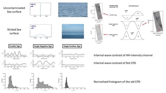
In this subsection, we analyze the results associated to the IW contrast profiles, which were classified into three different IW signature types, i.e., double sign, single-negative and positive. Please, see the thread 1 in the flowchart (Figure 3). The calculated $\Delta$ values for each IW contrast profiles composing our data set is shown in

Table 2. General view of the IW signature patterns and associated parameters. The double sign and single-negative and -positive signatures are presented, respectively as $+\setminus -$, −, and +.

Image ID	Profile ID	Signature Pattern	${\mathsf{\Delta }}_{{\mathit{\sigma }}_{\mathit{HH}}^0}$	${\mathsf{\Delta }}_{{\mathit{\sigma }}_{\mathit{VV}}^0}$	${\mathsf{\Delta }}_{{\mathit{\sigma }}_{\mathit{\varphi }\mathit{CPD}}}$	Correlation
1	1	$+\setminus -$	3.15	2.69	1.32	0.83
2	2	+	0.80	0.77	0.61	0.19
3	3	−	1.11	1.12	2.59	0.90
4	4	$+\setminus -$	1.99	1.80	0.84	0.34
5	5.1	+	0.47	0.39	0.20	0.13
	5.2	−	1.02	0.95	0.73	0.88
6	6	$+\setminus -$	0.77	0.62	0.31	0.38
7	7	$+\setminus -$	1.61	1.44	1.07	0.83
8	8	−	1.47	1.35	1.94	0.88
9	9.1	$+\setminus -$	2.10	1.67	0.97	0.27
	9.2	−	1.36	1.23	1.74	0.81

. Please, note that the ${\Delta }_{{\sigma }_{HH}^0}$ is higher than the ${\Delta }_{{\sigma }_{VV}^0}$ considering all profiles except the profile ID 3, which have ${\Delta }_{{\sigma }_{HH}^0}\approx {\Delta }_{{\sigma }_{VV}^0}$. Considering the tilted Bragg scattering (two-scale) model, higher IW HH-intensity modulations are expected [8,38]. Consequently, taking into account this rationality, the follow results are discussed considering only the HH-intensity channels. Furthermore, considering each IW profile, the correlations between ${\delta }_{{\sigma }_{HH}^0}$ and ${\delta }_{{\sigma }_{\varphi CPD}}$ are calculated and the results are also presented in Table 2.

• Double sign IW signatures
  We identify 5 HH-polarized contrast profiles that follow the double sign IW signature pattern. The ${\delta }_{{\sigma }_{HH}^0}$ profiles and their respective ${\delta }_{{\sigma }_{\varphi CPD}}$ are shown in Figure 5. Further details are listed in Table 2. The ${\delta }_{{\sigma }_{HH}^0}$ profiles have positive signatures more than 33% stronger than the negative ones. Please note that the ${\delta }_{{\sigma }_{\varphi CPD}}$ peaks are associated to the ${\delta }_{{\sigma }_{HH}^0}$ pits. As explained by the hydrodynamic theory related to IWs [3], the front and rear slope of the solitary wave are associated, respectively, with increasing and decreasing sea surface roughness (i.e., respectively, bright and dark band in SAR imagery). Considering the IW rear slope, the decreasing in the signal backscattered of the sea surface causes a consequent decreasing in the SNR values. Thus, since, as pointed by [21,22,23,39], the ${\sigma }_{\varphi CPD}$ over the sea surface tends to increase with decreasing SNR, the IW front and rear slopes are associated, respectively, with lower and higher ${\delta }_{{\sigma }_{\varphi CPD}}$ values (i.e., dark and bright bands in the ${\delta }_{{\sigma }_{HH}^0}$ images). The ${\Delta }_{{\sigma }_{HH}^0}$ varies between 0.77 and 3.15. Considering all IW signature profiles, the ${\Delta }_{{\sigma }_{\varphi CPD}}$ values are less than 50% lower than the ${\Delta }_{{\sigma }_{HH}^0}$ ones, i.e., varies between 0.31 and 1.32. The correlation between the ${\delta }_{{\sigma }_{HH}^0}$ and ${\delta }_{{\sigma }_{\varphi CPD}}$ values varies between 0.27 and 0.83, for double sign signatures.
• single-negative IW signatures
  Considering the single-negative signatures, 4 HH-polarized contrast profiles of our data set correspond to this class (or kind) of signature. The ${\delta }_{{\sigma }_{HH}^0}$ profiles and their corresponding ${\delta }_{{\sigma }_{\varphi CPD}}$ are depicted in Figure 6. The ${\delta }_{{\sigma }_{HH}^0}$ are mostly negative, as expected; while, the ${\delta }_{{\sigma }_{\varphi CPD}}$ are mostly positive. The ${\Delta }_{{\sigma }_{HH}^0}$ varies between 1.02 (Image ID 5) and 1.47 (Image ID 8). Please, see Table 2. The ${\Delta }_{{\sigma }_{\varphi CPD}}$ varies between 0.73 and 2.59. Note that, the ${\Delta }_{{\sigma }_{\varphi CPD}}$ are more than 22% higher than the corresponding ${\Delta }_{{\sigma }_{HH}^0}$ considering the range-propagating IW signatures, (i.e., Image ID 3, 8 and 9). The possible explanation for the higher ${\Delta }_{{\sigma }_{\varphi CPD}}$ associated to those single-negative IW signatures is the coupled effect of the hydrodynamic modulation (as discussed previously for the IW double sign signatures) and the role of surfactant films that enhance the co-polarized channel decorrelation, increasing the ${\sigma }_{\varphi CPD}$ values associated to the IW rear slope signatures. As demonstrated in [6], the IW negative contrast in radar power is stronger as surfactant film concentration (or film elasticity) increases. In another way, Image ID 5 has ${\Delta }_{{\sigma }_{\varphi CPD}}$ 30% lower than its corresponding ${\Delta }_{{\sigma }_{HH}^0}$. It is important to point out that the IW signature in Image ID 5 is propagating in azimuth direction. As discussed by [6], the azimuth-propagating IW signatures are many times dominated by single-negative signatures. We recall that we use the same model in [6] to explain the class of signatures reported in this paper. In the particular case of azimuthally propagating IWs, positive contrast variations are absent in the model, and the backscatter contrast is expected to be negative, in agreement with the observation in Figure 6b (top panel). This is a consequence of assuming Bragg scattering and hence the IW hydrodynamic modulation does not change significantly range propagating Bragg waves for azimuth propagating IWs. Thus, the lower values of ${\Delta }_{{\sigma }_{\varphi CPD}}$ in this case can be explained by the fact that the increasing decorrelation between the co-polarized channels associated to the IW rear slopes are due only to the surface film modulation effect.
  Please note that considering all single-negative IW signatures, the maximum and minimum ${\delta }_{{\sigma }_{\varphi CPD}}$ values are associated to the IW troughs and crests, respectively, and the correlation between the ${\delta }_{{\sigma }_{HH}^0}$ and ${\delta }_{{\sigma }_{\varphi CPD}}$ values are always higher than 0.81, for single-negative IW contrast.
• single-positive IW signatures
  We identify 2 HH-polarized contrast profiles that follow the single-positive IW signature. The ${\delta }_{{\sigma }_{HH}^0}$ profiles and their corresponding ${\delta }_{{\sigma }_{\varphi CPD}}$ are depicted in Figure 7. As expected, the ${\delta }_{{\sigma }_{HH}^0}$ values are mostly positive; while, considering image ID 2, the ${\delta }_{{\sigma }_{\varphi CPD}}$ signatures have a double sign pattern and, for image ID 5, the ${\delta }_{{\sigma }_{\varphi CPD}}$ values are mostly negative. The ${\Delta }_{{\sigma }_{HH}^0}$ are 0.80 (Image ID 2) and 0.47 (Image ID 5). Please, see Table 2. The ${\Delta }_{{\sigma }_{\varphi CPD}}$ for Image ID 2 and Image ID 5 are, respectively, 0.61 and 0.20, i.e., more than 23% lower than the ${\Delta }_{{\sigma }_{HH}^0}$. According to [6], when the wind speed is very low (<2 m/s), the IW can be imaged as bright bands only since the expected dark bands are lost in the dark SAR image background. Another complementary theory presented in [40] associates the IW single-positive signatures to either or both the following mechanisms: (1) generation of bound centimeter-decimeter waves with Bragg wavelengths; and (2) wave breaking. The latter mechanisms are the responsible by a positive contrast even on the IW rear slope due to the indirect contribution of meter-scale waves to the backscattered signal [41]. We note in passing that some advanced radar imaging models use a composite surface expansion, which account for long-wave–short-wave interaction terms resulting in upwind–downwind differences of the backscattered signal, and hence could explain single-positive signatures [42]. Thus, no decreasing in the sea surface backscattering related to the IW rear slope is expected as well as no increasing decorrelation between the co-polarized channels (consequently, no decreasing in the SNR values are expected), resulting in no clear modulation of the ${\sigma }_{\varphi CPD}$. Please note that, since Image ID 2 and Image ID 5 are not acquired under low wind condition (see Table 1), the second theory (i.e., the one accounting for wave breaking) is more reliable. Considering both images there is no clear correlation between ${\delta }_{{\sigma }_{HH}^0}$ and ${\delta }_{{\sigma }_{\varphi CPD}}$. This is confirmed by the lowest correlation between the ${\delta }_{{\sigma }_{HH}^0}$ and ${\delta }_{{\sigma }_{\varphi CPD}}$ (lower than 0.20).

In order to better understand the behavior of the std CPD associated to each type of IW contrast profiles, normalized histograms were computed and the results are shown in Figure 8. It is important to highlight that, for computing the histogram related to the IW single-negative sign signature, the azimuth-propagating IW image was not considered (because of its anomalous behavior as pointed out previously). It can be noted that the empirical statistical distribution of std CPD is different for each kind of IW contrast profile. For the double sign signatures (please, see Figure 8a), more than 50% of the std CPD values are concentrated between the range of 20° and 35°, being the mean and std values, respectively, 30° and 10°. Considering the single-negative sign signatures (see Figure 8b), the histogram is shifted to higher std CPD values, i.e., more than 50% of the std CPD values are concentrated within the range of 22° to 52°. Furthermore, the histogram becomes wider, with mean and std values of, respectively, 47° and 20°. The single-positive sign signatures (see Figure 8c) are associated to the most left-shifted histogram (i.e., shifted to lower std CPD values, with more than 50% of the std CPD values being within the range of 22° to 26°) as well as it has the narrowest histogram (mean and std values of, respectively, 24° and 4°). Since higher std CPD values are expected over the sea surface under the influence of slicks [19,20,21,43], the results related to the histograms analysis confirm the previous outcomes in this paper, principally, regarding the possible influence of surfactant films on the IW single-negative sign signatures.

4.2. Signal to Noise Ratio Analysis

In this subsection, we present the analysis of the SNR for each IW contrast profile of our data set. Please see the thread 2 in the flowchart presented in Figure 3. It was discussed in previous studies the manifestations of film slick formation related to IWs as well as the impact of those films on the IW signatures in SAR imagery [6,9]. In order to interpret the SAR imagery of IWs and to understand the role of film slicks in their signatures, the SNR must be accounted for. Hence, the SNR is calculated using the nominal NESZ associated to the APL sensor at off nadir angle 21.5° [44]. For each IW profile, we split the ${\sigma }^0$ values into two different classes, i.e., crests and troughs.

Figure 9 shows the SNR associated to the IW crests and troughs for each profile. The results are presented in the graphical format known as box plot, where the median SNR is represented by the horizontal line inside the box, while the first ($Q_1$) and third quartiles ($Q_3$) are, respectively, the lower and upper lines of the box. The minimum and maximum values excluding outliers are, respectively, the lower and higher short horizontal bars. The minimum and maximum values are calculated, respectively, using $Q_1-1.5IQR$ and $Q_3+1.5IQR$, where IQR is the interquartile range (i.e., $IQR=Q_3-Q_1$). Since we have identified three different types of HH-polarized contrast profiles, ${\delta }_{{\sigma }_{HH}^0}$, in our data set, i.e., double (Figure 9a) and single-negative and -positive signatures (respectively, Figure 9b,c), the results are organized according to the type of IW signature. Please note that the SNR associated to the VV channel is also shown, as well as the dashed red line representing the 3 dB threshold (below this threshold we consider the measurements as very low signal samples).

As expected, the median HH-channel SNR associated to the IW troughs are lower than the crests, consistently for all profiles. Considering the IW double sign signatures (Figure 9a), the SNR values are well above the 3 dB threshold for both IW crests and troughs. The SNR values associated to the IW single-negative signature profiles (Figure 9b) are well above the threshold for IW crests as well as for the IW troughs associated to Image 5 and 9; while, the SNR values are near the threshold for Image ID 8 and fall below the threshold for Image ID 3. The SNR values associated to single-positive signatures (Figure 9c) are well above the threshold considering both crests and troughs.

The highest separation in SNR statistics between IW crests and troughs are found for single-negative sign signatures; while, for single-positive signatures, the SNRs are very near for both crests and troughs. Note that, as expected, higher SNR values separability between the IW crest and troughs classes are associated to higher ${\delta }_{{\sigma }_{\varphi CPD}}$ modulation and higher correlation between the ${\delta }_{{\sigma }_{HH}^0}$ and ${\delta }_{{\sigma }_{\varphi CPD}}$ values. The SNR variability (i.e., the SNR standard deviation) associated to the IW troughs is higher than to the crests considering all profiles. The difference between the SNR variability associated to the IW crests and troughs is more evident for the single-negative signatures (Figure 9b), excluding Image ID 5, where IWs travel in azimuth direction. The difference is less evident for the single-positive signatures. As discussed previously maybe the large SNR variability associated to the single-negative signatures is mainly due to the damping properties of the surfactant layer that varies in space along the IW trains, and consequently along IW propagation direction (i.e., the surfactant concentration is different for the different solitons in the same IW train [9]) causing the large SNR variability related to the single-negative IW trough’s signatures, see Figure 9. This variability associated to the different damping properties of the surfactant layer is also discussed by [45]. The same analysis applies for VV channel. Please note that, as pointed out in other studies [23,45], the VV channel is less noise corrupted considering all profiles.

4.3. Biomass Production Validation

We present in this section the analysis of the chlorophyll-a maps associated to each SAR image of our data set as presented in the thread 3 in the flowchart, Figure 3. The biomass production by marine organisms in the oceanic environment, principally phytoplankton, is pointed out by marine biologists as the largest source of natural surfactant films at the sea surface [12,46]. Several studies discuss the capability of phytoplankton for producing surface-active materials as metabolic by-products [12,13]. The in situ production of organic substances by plankton and bacteria are the most important source of surface-active material in the marine environment and only about 10% of surfactants own their existence to anthropogenic input [47]. Laboratorial experiments conducted by [12] showed that surfactants are produced in culture media of species of marine phytoplankton depending on the age of culture and species. These authors conducted field experiments showing a positive correlation between surfactant activity in seawater column and phytoplankton production at several northern Adriatic Sea stations. Furthermore, space borne radar scatterometers have shown a strong reduction of the Normalized Radar Cross Section (NRCS) (6 to 20 dB) in areas where ocean color data show a high chlorophyll-a concentration [48]. In [49] it has been suggested that, natural slick coverage can be used as a proxy for ocean productivity. Here, we consider chlorophyll-a concentration as a proxy to the enhancement of surfactant film concentration (in more technical language, enhanced surface film pressure).

Figure 10 shows the CHL-a concentration associated to each SAR image of our data set. The results are presented in a graphical format known as box plot. The outliers are represented by the red plus signs. The outliers are considered when the elements are >1.5$IQR$ below the first quartile or above the third quartile. The sections with gray background are the ones identified as single-negative signatures of IWs propagating in range direction. The yellow background sections mean that the chlorophyll-a images are not useful owing to cloud coverage. Considering the double sign and single-positive IW signature types, the maximum CHL-a concentration excluding outliers is associated to Image ID 1 (0.87 mg/m³). It is important to highlight that the CHL-a product related to Image ID 1 is very cloud-covered, with contaminated pixels being about 50%. Therefore the value should be considered with caution. In fact we discard this measurement. For all the other images following these signature types, excluding outliers, the maximum CHL-a concentration is always equal or lower than 0.57 mg/m³. The values of CHL-a concentrations associated to the single-negative signatures with IWs traveling in the range direction (i.e., Image ID 3, 8, and 9, gray sections in Figure 10) have maximum CHL-a concentrations excluding outliers always equal or higher than 0.63 mg/m³ (Image ID 8). Excluding outliers, the maximum CHL-a concentration is found for Image ID 3, i.e., 1.1 mg/m³. Furthermore, the statistical distribution of the CHL-a concentration associated to these images are more evidently right-skewed than the others. Image ID 5, where the IW is traveling in the azimuth direction, is associated to the lower values of CHL-a concentration for the single-negative signatures. The latter image has maximum CHL-a concentration of 0.41 mg/m³. However, it is important to point out the CHL-a product for this image is jeopardized due to intense cloud-coverage, since the contaminated pixels are about 60%.

We note that, in general, the single-negative IW signatures (gray sections in Figure 10) present higher chlorophyll-a values, which also have a much larger number of outliers. We attribute the outlier values to possible phytoplankton blooms, which are translated into higher chlorophyll-a values. Note that the images are Level 3 monthly, indicating, in our view, that the outliers are true values, but not bad data. Hence, it is suggested that the elevated values of chlorophyll-a concentration in Image IDs 3, 8, and 9 are an indication of enhanced concentration of surfactant films. We stress that, this is consistent with our hypothesis for explaining the single-negative “dark-banded” IW signatures.

Figure 11 shows the frames of the SAR images associated to the IW single-negative sign signature overlaid onto the productive habitats of the GMR mapped by [34]. Please, note that the SAR scenes were acquired near the productive habitats. The IW profiles that have higher ${\Delta }_{{\sigma }_{\varphi CPD}}$ values (i.e., Image IDs 3, 8, and 9) are associated with SAR images acquired in March. To the south of 0.75°N, a biomass peak is observed around March [34], as presented previously in Section 3. These SAR images were also acquired during a weak and strong La Niña event, respectively, 2008/2009 (associated to Image ID 3) and 2010/2011 (associated to Image IDs 8 and 9).

5. Conclusions

A study aimed at investigating the IW signatures in SAR imagery by means of the polarimetric feature named std CPD was performed for the first time in literature. Experiments on actual SAR measurements were accomplished considering 9 L-band ALOS-PALSAR polarimetric scenes. The IW patterns were classified according to 3 different types of IW contrast profiles, i.e., double sign and single-negative and -positive signatures. The main outcomes of this study are summarized as follows:

• Considering the IW double sign signatures, the modulation associated to the std CPD is lower than the one associated to the HH- and VV-polarized intensity channels. The decreasing correlation between the co-polarized channels on the IW rear slope (higher std CPD values) is presumably due to the lower sea surface roughness (caused by hydrodynamic modulation) and, consequently, lower SNR.
• Taking into account the IW single-negative sign signatures, the modulation associated to the std CPD is higher than the one associated to HH- and VV-polarized intensity channels for the range-propagating IW signatures. Probably, the reason is the coupled effect of the hydrodynamic modulation and the surfactant films associated to the IW rear slopes and over the IW troughs, which admittedly decreases the correlation between the co-polarized channels (causing the raise of the std CPD values). In other way, for the azimuth-propagating IW signature, the std CPD is lower than the one associated to the HH-polarized intensity channel. The likely explanation is that the decreasing correlation between the co-polarized channels (and, consequently, the increase of the std CPD values) are mostly due to only one effect, i.e., the surfactant films present in the IW rear slope and over the IW trough.
• For the IW single-positive sign signatures, the modulation associated to the std CPD is lower than the one associated to the HH- and VV-polarized intensity channels. Since no decreasing in the IW rear slope sea surface backscattering is expected, no clear modulation of the std CPD is observed.

In this study we apply the same classification scheme used in [6] for C-band SAR images to IW signatures observed with the L-band ALOS-PALSAR. In [6], it was demonstrated that IWs appear as dark bands on a gray background in the presence of surface films, which were classified as single-negative sign signatures. In this study too, we observe dark signatures on a gray background for L-Band, and use the same classification scheme. We note in passing that the single-negative sign signatures were found in highly productive hot-spots off the Galapagos Islands, i.e., in the island-wakes prone to upwelling and in certain seasons. Nevertheless, this possible connection between surfactants from biologically productive areas and IW signatures needs further investigations.

The outcomes described in this paper may support the design of algorithms aimed at IWs automatic extraction and classification based on co-polarized coherent SAR measurement and the design of polarimetric SAR architectures that aim at observing a wide range of ocean features (e.g., ripples, oceanic fronts, river plumes, and IWs). In future work we may include the organization of field campaigns coincident with satellite SAR acquisitions, aimed at sampling surfactant films on the sea surface associated to IW features, and the extension of such analysis to a larger data set. The latter should include SAR images acquired with higher incidence angles and under different wind regimes such as very low and/or very high wind speed, as well as the use of SAR scenes acquired by different polarimetric sensors working in different frequencies (e.g., X- and C- Bands).

References

1. Jackson, C.R.; Da Silva, J.C.; Jeans, G. The generation of nonlinear internal waves. Oceanography 2012, 25, 108–123. [Google Scholar] [CrossRef]
2. Muacho, S.; Da Silva, J.; Brotas, V.; Oliveira, P. Effect of internal waves on near-surface chlorophyll concentration and primary production in the Nazaré Canyon (west of the Iberian Peninsula). Deep Sea Res. Part I Oceanogr. Res. Pap. 2013, 81, 89–96. [Google Scholar] [CrossRef]
3. Alpers, W. Theory of radar imaging of internal waves. Nature 1985, 314, 245–247. [Google Scholar] [CrossRef]
4. Apel, J.R. Oceanic internal waves and solitons. In An Atlas of Oceanic Internal Solitary Waves; Global Ocean Associates: Alexandria, VA, USA, 2002; pp. 1–40. [Google Scholar]
5. Magalhaes, J.M.; Da Silva, J.C.B.; Buijsman, M.C.; Garcia, C.A.E. Effect of the North Equatorial Counter Current on the generation and propagation of internal solitary waves off the Amazon shelf (SAR observations). Ocean Sci. 2016, 12, 243. [Google Scholar] [CrossRef] [Green Version]
6. Da Silva, J.; Ermakov, S.; Robinson, I.; Jeans, D.; Kijashko, S. Role of surface films in ERS SAR signatures of internal waves on the shelf: 1. Short-period internal waves. J. Geophys. Res. Ocean. 1998, 103, 8009–8031. [Google Scholar] [CrossRef]
7. Jackson, C.R.; da Silva, J.C.; Jeans, G.; Alpers, W.; Caruso, M.J. Nonlinear internal waves in synthetic aperture radar imagery. Oceanography 2013, 26, 68–79. [Google Scholar] [CrossRef] [Green Version]
8. Kudryavtsev, V.; Kozlov, I.; Chapron, B.; Johannessen, J. Quad-polarization SAR features of ocean currents. J. Geophys. Res. Ocean. 2014, 119, 6046–6065. [Google Scholar] [CrossRef] [Green Version]
9. Ermakov, S.; Salashin, S.; Panchenko, A. Film slicks on the sea surface and some mechanisms of their formation. Dyn. Atmos. Ocean. 1992, 16, 279–304. [Google Scholar] [CrossRef]
10. Gade, M.; Hühnerfuss, H.; Korenowski, G. Marine Surface Films; Springer: Berlin, Germany, 2006; Volume 1243. [Google Scholar]
11. Ermakov, S.A.; Sergievskaya, I.A.; Da Silva, J.C.; Kapustin, I.A.; Shomina, O.V.; Kupaev, A.V.; Molkov, A.A. Remote Sensing of Organic Films on the Water Surface Using Dual Co-Polarized Ship-Based X-/C-/S-Band Radar and TerraSAR-X. Remote Sens. 2018, 10, 1097. [Google Scholar] [CrossRef] [Green Version]
12. Žutić, V.; Ćosović, B.; Marčenko, E.; Bihari, N.; Kršinić, F. Surfactant production by marine phytoplankton. Mar. Chem. 1981, 10, 505–520. [Google Scholar] [CrossRef]
13. Kujawinski, E.B.; Farrington, J.W.; Moffett, J.W. Evidence for grazing-mediated production of dissolved surface-active material by marine protists. Mar. Chem. 2002, 77, 133–142. [Google Scholar] [CrossRef]
14. Wurl, O.; Miller, L.; Röttgers, R.; Vagle, S. The distribution and fate of surface-active substances in the sea-surface microlayer and water column. Mar. Chem. 2009, 115, 1–9. [Google Scholar] [CrossRef]
15. Hühnerfuss, H.; Alpers, W.; Jones, W.L.; Lange, P.A.; Richter, K. The damping of ocean surface waves by a monomolecular film measured by wave staffs and microwave radars. J. Geophys. Res. Ocean. 1981, 86, 429–438. [Google Scholar] [CrossRef]
16. Alpers, W.; Hühnerfuss, H. The damping of ocean waves by surface films: A new look at an old problem. J. Geophys. Res. Ocean. 1989, 94, 6251–6265. [Google Scholar] [CrossRef]
17. Dierking, W.; Skriver, H.; Gudmandsen, P. SAR polarimetry for sea ice classification. In Proceedings of the Workshop on POLinSAR—Applications of SAR Polarimetry and Polarimetric Interferometry, Frascati, Italy, January 2003; Volume 529. [Google Scholar]
18. Migliaccio, M.; Nunziata, F.; Buono, A. SAR polarimetry for sea oil slick observation. Int. J. Remote Sens. 2015, 36, 3243–3273. [Google Scholar] [CrossRef] [Green Version]
19. Migliaccio, M.; Nunziata, F.; Gambardella, A. On the co-polarized phase difference for oil spill observation. Int. J. Remote Sens. 2009, 30, 1587–1602. [Google Scholar] [CrossRef]
20. Velotto, D.; Migliaccio, M.; Nunziata, F.; Lehner, S. Dual-polarized TerraSAR-X data for oil-spill observation. IEEE Trans. Geosci. Remote Sens. 2011, 49, 4751–4762. [Google Scholar] [CrossRef]
21. Buono, A.; Nunziata, F.; de Macedo, C.R.; Velotto, D.; Migliaccio, M. A sensitivity analysis of the standard deviation of the Copolarized phase difference for sea oil slick observation. IEEE Trans. Geosci. Remote Sens. 2018, 57, 2022–2030. [Google Scholar] [CrossRef]
22. Buono, A.; de Macedo, C.R.; Nunziata, F.; Velotto, D.; Migliaccio, M. Analysis on the Effects of SAR Imaging Parameters and Environmental Conditions on the Standard Deviation of the Co-Polarized Phase Difference Measured over Sea Surface. Remote Sens. 2019, 11, 18. [Google Scholar] [CrossRef] [Green Version]
23. Espeseth, M.M.; Brekke, C.; Jones, C.E.; Holt, B.; Freeman, A. The impact of system noise in polarimetric SAR imagery on oil spill observations. IEEE Trans. Geosci. Remote Sens. 2020, 58, 4194–4214. [Google Scholar] [CrossRef]
24. Guissard, A. Mueller and Kennaugh matrices in radar polarimetry. IEEE Trans. Geosci. Remote Sens. 1994, 32, 590–597. [Google Scholar] [CrossRef]
25. Ulaby, F.; Sarabandi, K.; Nashashibi, A. Statistical properties of the Mueller matrix of distributed target. IEE Proc.-F 1992, 139, 136–146. [Google Scholar]
26. Joughin, I.R.; Winebrenner, D.P.; Percival, D.B. Probability density functions for multilook polarimetric signatures. IEEE Trans. Geosci. Remote Sens. 1994, 32, 562–574. [Google Scholar] [CrossRef]
27. Lee, J.S.; Hoppel, K.W.; Mango, S.A.; Miller, A.R. Intensity and phase statistics of multilook polarimetric and interferometric SAR imagery. IEEE Trans. Geosci. Remote Sens. 1994, 32, 1017–1028. [Google Scholar]
28. Schuler, D.; Lee, J.S. Mapping ocean surface features using biogenic slick-fields and SAR polarimetric decomposition techniques. IEEE Proc. Radar Sonar Navig. 2006, 153, 260–270. [Google Scholar] [CrossRef]
29. Jackson, C.R.; Apel, J. An atlas of internal solitary-like waves and their properties. Contract 2004, 14, 0176. [Google Scholar]
30. Magalhaes, J.M.; Da Silva, J.C. Internal solitary waves in the Andaman Sea: New insights from SAR imagery. Remote Sens. 2018, 10, 861. [Google Scholar] [CrossRef] [Green Version]
31. Osborne, A.; Burch, T. Internal solitons in the Andaman Sea. Science 1980, 208, 451–460. [Google Scholar] [CrossRef]
32. Doydee, P.; Saitoh, S.I.; Matsumoto, K. Variability of chlorophyll-a and SST at regional seas level in Thai waters using satellite data. J. Fish. Environ. 2010, 34, 35–44. [Google Scholar]
33. Suwannathatsa, S.; Wongwises, P. Chlorophyll distribution by oceanic model and satellite data in the Bay of Bengal and Andaman Sea. Oceanol. Hydrobiol. Stud. 2013, 42, 132–138. [Google Scholar] [CrossRef]
34. Schaeffer, B.A.; Morrison, J.M.; Kamykowski, D.; Feldman, G.C.; Xie, L.; Liu, Y.; Sweet, W.; McCulloch, A.; Banks, S. Phytoplankton biomass distribution and identification of productive habitats within the Galapagos Marine Reserve by MODIS, a surface acquisition system, and in-situ measurements. Remote Sens. Environ. 2008, 112, 3044–3054. [Google Scholar] [CrossRef]
35. Witman, J.D.; Brandt, M.; Smith, F. Coupling between subtidal prey and consumers along a mesoscale upwelling gradient in the Galapagos Islands. Ecol. Monogr. 2010, 80, 153–177. [Google Scholar] [CrossRef] [Green Version]
36. Kanamitsu, M.; Ebisuzaki, W.; Woollen, J.; Yang, S.K.; Hnilo, J.; Fiorino, M.; Potter, G. Ncep–doe amip-ii reanalysis (r-2). Bull. Am. Meteorol. Soc. 2002, 83, 1631–1644. [Google Scholar] [CrossRef]
37. NASA Goddard Space Flight Center; Ocean Ecology Laboratory; Ocean Biology Processing Group. Moderate-Resolution Imaging Spectroradiometer (MODIS) Aqua Chlorophyll a Data. Available online: https://oceandata.sci.gsfc.nasa.gov/MODIS-Aqua/Mapped/Monthly/4km/chlor_a/ (accessed on 7 July 2020).
38. Kudryavtsev, V.; Hauser, D.; Caudal, G.; Chapron, B. A semiempirical model of the normalized radar cross-section of the sea surface 1. Background model. J. Geophys. Res. Ocean. 2003, 108, FET-2. [Google Scholar] [CrossRef] [Green Version]
39. Alpers, W.; Holt, B.; Zeng, K. Oil spill detection by imaging radars: Challenges and pitfalls. Remote Sens. Environ. 2017, 201, 133–147. [Google Scholar] [CrossRef]
40. Da Silva, J.; Ermakov, S.; Robinson, I.; Potter, R. ERS SAR observations of long internal waves with positive backscatter signatures. In Proceedings of the IEEE 1999 International Geoscience and Remote Sensing Symposium. IGARSS’99 (Cat. No. 99CH36293), Hamburg, Germany, 28 June–2 July 1999; Volume 3, pp. 1481–1483. [Google Scholar]
41. Thompson, D.; Gasparovic, R. Intensity modulation in SAR images of internal waves. Nature 1986, 320, 345–348. [Google Scholar] [CrossRef]
42. Brandt, P.; Romeiser, R.; Rubino, A. On the determination of characteristics of the interior ocean dynamics from radar signatures of internal solitary waves. J. Geophys. Res. Ocean. 1999, 104, 30039–30045. [Google Scholar] [CrossRef] [Green Version]
43. Skrunes, S.; Brekke, C.; Jones, C.E.; Holt, B. A multisensor comparison of experimental oil spills in polarimetric SAR for high wind conditions. IEEE J. Sel. Top. Appl. Earth Obs. Remote Sens. 2016, 9, 4948–4961. [Google Scholar] [CrossRef] [Green Version]
44. Earth Observation Research and Application Center JAXA. ALOS Data Users Handbook, Revision C; Earth Observation Research and Application Center JAXA: Tokyo, Japan, 2008. [Google Scholar]
45. Nunziata, F.; de Macedo, C.; Buono, A.; Velotto, D.; Migliaccio, M. On the analysis of a time series of X–band TerraSAR–X SAR imagery over oil seepages. Int. J. Remote Sens. 2019, 40, 3623–3646. [Google Scholar] [CrossRef]
46. Wilson, W.; Collier, A. The production of surface-active material by marine phytoplankton cultures. J. Mar. Res. 1972, 30, 15–26. [Google Scholar]
47. Gašparović, B.; Kozarac, Z.; Saliot, A.; Ćosović, B.; Möbius, D. Physicochemical Characterization of Natural Andex-Situ Reconstructed Sea-Surface Microlayers. J. Colloid Interface Sci. 1998, 208, 191–202. [Google Scholar] [CrossRef] [PubMed] [Green Version]
48. Lin, I.I.; Alpers, W.; Liu, W.T. First evidence for the detection of natural surface films by the QuikSCAT scatterometer. Geophys. Res. Lett. 2003, 30. [Google Scholar] [CrossRef] [Green Version]
49. Garrett, W. Physicochemical effects of organic films at the sea surface and their role in the interpretation of remotely sensed imagery. In ONRL Workshop Proceedings: Role of Surfactant Films on the Interfacial Properties of the Sea Surface; Office of Naval Research London Branch: London, UK, 1986; pp. 1–17. [Google Scholar]
Figure 1. L-band ALOS-PALSAR image acquired on 2009.03.14 showing an example of an internal wave (IW) near Galapagos Island. (a) HH-polarized intensity channel (i.e., σ H H 0 ) image, (b) VV-polarized intensity channel (i.e., σ V V 0 ) image, where the blue line represents the selected IW profile; and (c) IW profile associated to HH- and VV-polarized intensity channels, where the black and gray dashed lines correspond to the mean value of the background associated to, respectively, HH- and VV-polarized intensity.
Remotesensing 12 02372 g001
Figure 2. The HH-intensity (left) and standard deviation of co-polarized phase difference (CPD) (right) ALOS-PALSAR (APL) excerpt images showing IW signatures related to: (a) Image ID 2 acquired in Andaman Sea on 2007.04.14; (b) Image ID 3 acquired in Galapagos Marine Reserve (GMR) on 2009.03.14; and (c) Image ID 5 acquired in GMR on 2009.08.28. The selected IW profiles and ROI representing the backgrounds are depicted in blue lines and red rectangles, respectively. Please, note that the profile ID numbers are depicted in the figures. More information about the images can be found in Table 1.
Remotesensing 12 02372 g002
Figure 3. Flowchart of the methodological approach, where thread 1, 2, and 3 represent, respectively, the analysis of the IW contrast profiles according to the IW signature type, the analysis of the signal to noise ratio (SNR), and the investigation of the chlorophyll-a concentration maps associated to each SAR image of our data set.
Remotesensing 12 02372 g003
Figure 4. Scheme representing the IW signature type and the its SAR morphology. The dashed black line represents a homogeneous sea surface background. The IW phase velocity is represented by the C vector.
Remotesensing 12 02372 g004
Figure 5. δ σ H H 0 and δ σ ϕ C P D profiles (upper and lower, respectively) associated to: (a) Image ID 1; (b) Image ID 4; (c) Image ID 6; (d) Image ID 7; and (e) Image ID 9 (Profile ID 9.1). The dotted green lines show the δ = 0 ; where l = l 0 .
Remotesensing 12 02372 g005
Figure 6. δ σ H H 0 and δ σ ϕ C P D profiles (upper and lower, respectively) associated to: (a) Image ID 3; (b) Image ID 5 (Profile ID 5.2); (c) Image ID 8; and (d) Image ID 9 (Profile ID 9.2). The dotted green lines show the δ = 0 ; where l = l 0 .
Remotesensing 12 02372 g006
Figure 7. δ σ H H 0 and δ σ ϕ C P D profiles (upper and lower, respectively) associated to: (a) Image ID 2; and (b) Image ID 5 (Profile ID 5.1). The dotted green lines show the δ = 0 ; where l = l 0 .
Remotesensing 12 02372 g007
Figure 8. Normalized histograms of the std CPD associated to: (a) double sign signatures; (b) single-negative sign signatures; and (c) single-positive sign signatures.
Remotesensing 12 02372 g008
Figure 9. SNR values presented in the format of box plot for both HH- and VV-intensity, respectively, upper and lower panels. For each profile, the classes are divided in IW crest (left) and troughs (right): (a) double sign IW signatures; (b) single-negative sign IW signatures; and (c) single-positive sign IW signatures. Please note that, for each box plot, the horizontal line inside the box represents the median SNR values and its first and third quartiles are represented by the lower and upper line of the box. The minimum and maximum SNR values excluding outliers are represented by the lower and higher short horizontal bars. The dashed red line represents the 3 dB SNR threshold.
Remotesensing 12 02372 g009
Figure 10. Chlorophyll-a (CHL-a) concentration values presented in the format of box plot associated to each SAR image of our data set. Please note that, for each box plot, the horizontal line inside the box represents the median CHL-a concentration and its first and third quartiles are represented by the lower and upper line of the box. The minimum and maximum CHL-a concentrations excluding outliers are represented by the lower and higher short horizontal bars. The outliers are represented by the red plus signs. The sections with gray background are the ones identified as single-negative signatures of IWs propagating in range direction. The yellow background sections mean that the chlorophyll-a images are not useful owing to cloud coverage.
Remotesensing 12 02372 g010
Figure 11. Frames of the SAR images associated to the IW single-negative sign signature (blue rectangles) overlaid to the productive habitats of the GMR indicated as gray shaded regions. The red dots show the region where the IW profiles were extracted. Adapted from Figure 10 in [34].
Remotesensing 12 02372 g011