Comparative Study of IoT-Based Topology Maintenance Protocol in a Wireless Sensor Network for Structural Health Monitoring

Abstract

A structural health monitoring (SHM) system is an approach for identifying the damages caused to various kinds of structures using different system functions and providing the necessary feedback about structure’s conditions. As civil structures are the backbone of our society, to determine its daily operations is a very important issue. The performance measurement of those structures is manual whereas a computer-based monitoring system could automatically assess the structural damages and identify its exact location. Recently, wireless sensor networks (WSNs) have attracted a great deal of attention for remote sensing applications due to flexibility to measure of various activity of large scale network. Since technology is advancing day by day, the overall cost of a monitoring system is also decreased. However, the major challenging fact of a WSNs is to provide scalability for covering a large area. The main question is arisen how much capable have of a monitoring system to turn off unnecessary nodes to save energy while there are no events detected. To support the scalability required of an existing network and save the node energy for future use, we propose a topology maintenance protocol integrated with construction to address the issue of a node’s energy consumption by placing it optimally and extending the monitoring system’s lifetime. As per the authors’ acknowledgement that, a little attention has been paid to developing such a hybrid approach. To mitigate node energy consumption issue with large scale support, an Internet of Things (IoT)-based maintenance approach is the best candidate for obtaining better system lifetime responses. Therefore, the main goal of this work is to develop an ‘on-the-fly’-based topology maintenance monitoring system, which can maintain a network’s infrastructure while gathering a node’s information to switch its state regularly when the present network is no longer optimal.

1. Introduction

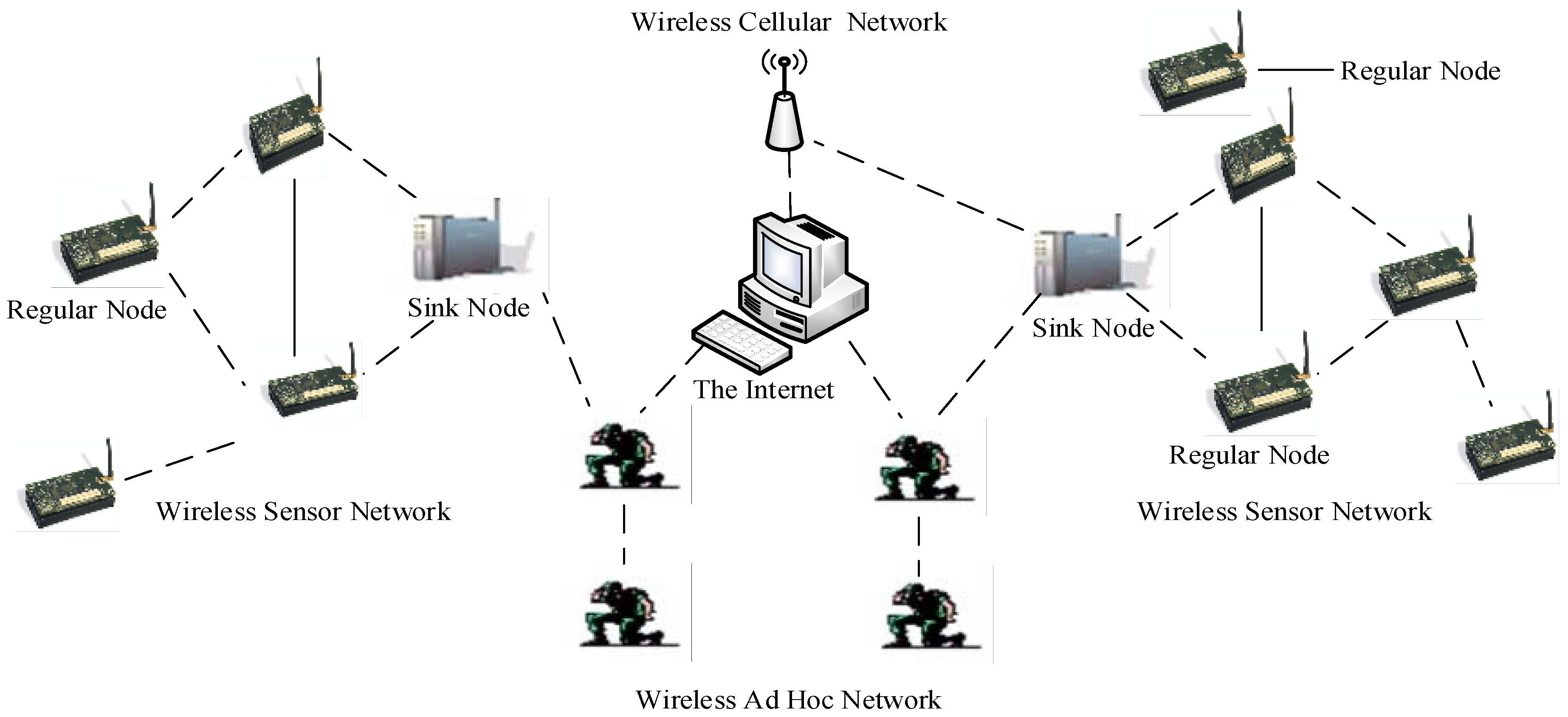
Structural health monitoring (SHM) is an emerging area of research that can automatically assess structural damage to buildings, aerospace vehicles, bridges, etc., with a system’s overall performance defined as changes to its material and/or geometric properties. Addressing several research problems in the multi-disciplinary research field has begun. Many researchers are trying to find a suitable method for resolving various challenging issues, such as the lifetime, scalability and maintenance of a remote sensing system, with wireless sensor networks (WSNs) providing the best solution for monitoring applications. In a real-time application, one of the big challenges concerning the monitoring of a large area is having an optimum salable network using 100 to 1000 nodes placed optimally. The general architecture of WSNs has been integrated with other technologies, such as wireless cellular networks, wireless ad hoc networks and other internet technologies, as depicted in Figure 1 [1] in which it can be seen that two types of wireless devices are usually used, a regular node and a sink. The number of applications of WSNs is constantly increasing, with new fields introduced by researchers. 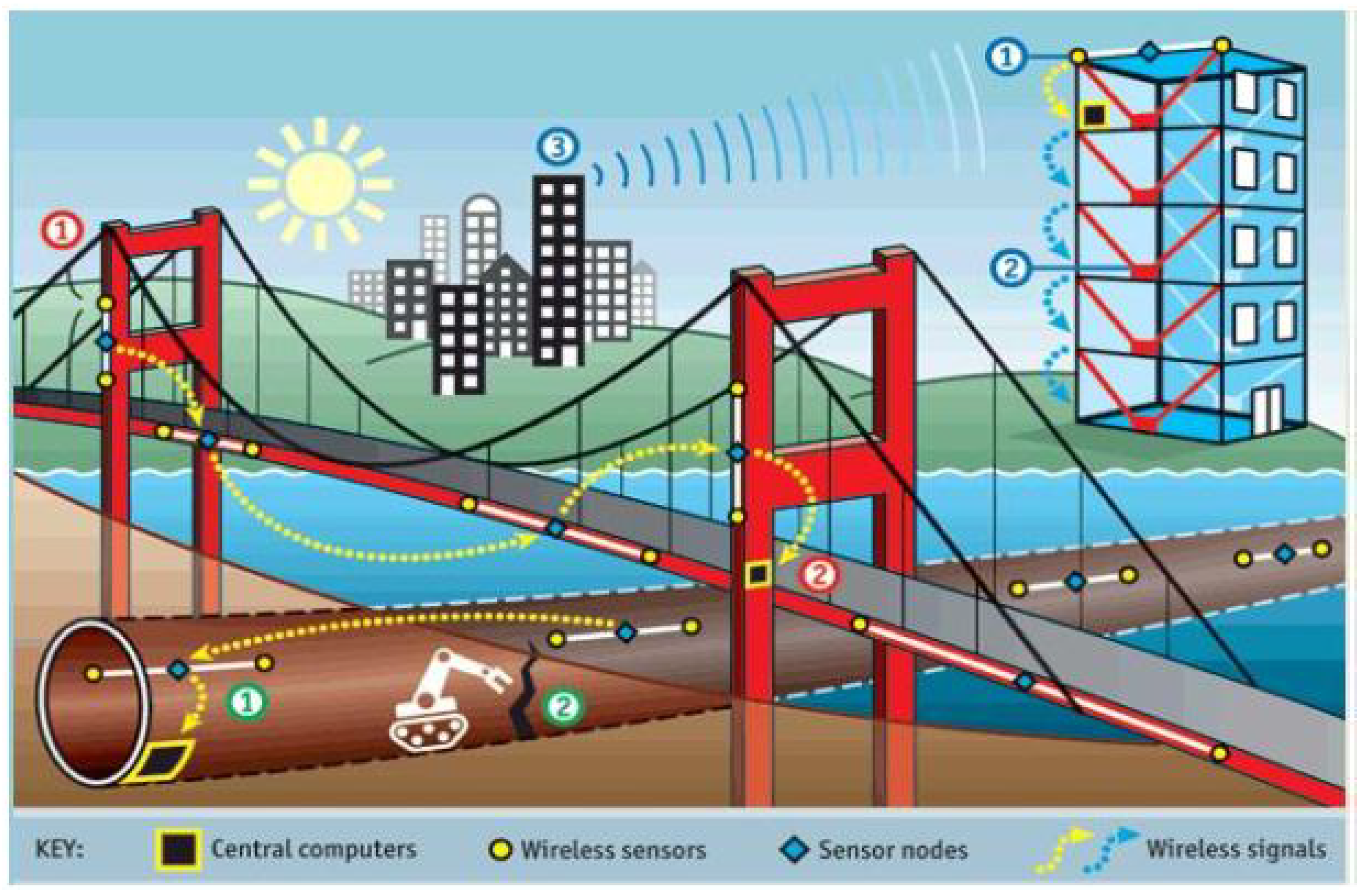In recent years, research on unmanned aerial vehicles (UAVs) and the industrial-based Internet of Things (IoT) [2,3,4] that considers the quality of service (QoS) aware data has attracted interest in WSNs [5,6,7]. An overview of SHM systems for various types of infrastructures, such as bridges, buildings and tunnels, using WSNs is illustrated in Figure 2 [1]. Generally, each monitoring system consists of three kinds of sections for the area of monitoring interest namely sensing, data transmission and computation. Since all of those above activities use the power from the sensor node energy where the battery is the main source, among those, data collection system from field sensor nodes plays a vital rule that determines the whole system aliveness for structural health monitoring. In the case of a building monitoring system, its deformations occur due to catastrophic events such as strong winds, earthquakes and other natural calamities [8].

To minimize structural damage, mass and shock absorbers methods have been used. During an earthquake, the accelerometer range should be in the range of 1–2 g to measure seismic intensity. Although, that measurement is more sensitive and most of the time interrupted by traffic and wind energy, which is in the order of ten to hundreds of micro of acceleration. In the bridge monitoring system, an earthquake detection system could generate an alarm and send it to its nearby station to provide awareness of an event’s characteristics. In a bridge monitoring system, various phenomena, such as vibrations and cracks, are detected by its associated field sensor, with the information acquired then transmitted over a short or long distance to identify the exact problem [9]. In the meantime, its detection system finds the problem during the event and sends a warning to the control system to take appropriate action before the entire system is damaged. In addition, WSNs are applied in tunnel systems to monitor safety by tracking events, such as a fire or other kind of intrusion, at their exact locations [10].

In the field of SHM, applying sensor networks is increasing daily due to technological advancements and their low implementation costs. Generally, their sensor nodes collect data from the field and send them to a base station using a proper network architecture and algorithms and, finally, to an analysis section, with a wire-based data collection system the traditional approach for gathering sensed data as its longevity is greater than those of other systems. However, due to several problems, such as its high installation cost, this system has lost its popularity [1]. A system designer designs a monitoring system based on the characteristics of a particular event and, in the area of interest, many sensors have been placed to detect damage. For a surveillance system, a dynamic factor assumption is an approach for determining seismic intensity but its high implementation cost is its major drawback. On the other hand, a cognitive radio-based WSN for monitoring a building’s structural health (i.e., vibrations) has been proposed [11].

In this paper, we propose an IoT-based topology maintenance protocol in a WSN, since it has a major benefit to reconstruct a new topology to provide the required strength. We have tested the proposed system in an extensive simulation scenario, since every time those algorithms create new of the previous one using gather knowledge from its neighborhood node. At the initial phase of node connection, topology construction protocol is applied first. After that, when the present connected topology is no longer optimal, based on the collected data from the neighboring topology maintenance algorithm create a new version of the previous one with placing node optimally. It saves nodes’ energy by preserving important characteristics of the network such as its coverage and connectivity over its whole lifetime. After creating a minimal topology, the network begins to perform its designated tasks. Each activity is related to every other, builds a new one using previous data and allocates minimum resources considering the network cost. As not all nodes participate in gathering data, their energy is saved by keeping them in the sleep mode which is the aim of this work. The main objective of this research is to integrate an IoT-based maintenance protocol with an existing topology construction one as an advanced technology for saving the nodes energy and thereby maximizing the monitoring system’s lifetime. The features, strengths and weakness of each topology construction protocol are summarized in

Table 1. List of major features, strength and weakness for relevant protocols.

Protocol	Features	Strength	Weakness
EECDS	Use Prim’s algorithm and growing as a tree	Energy efficient	More complexity in message generation
CDS-Rule-K	Grow on coloring approach Use pruning mechanism.	Able to discard unnecessary node	Complexity in computation and message
A3	Simple and able to distribute energy energy	Synchronous is nor required	Less reliable with fewer node leave uncover area when small number of active node is used
A3 Cov	Address coverage area problem	Saving node energy specially care about Sensing coverage area	sensing coverage area is not very large

.

The remainder of this paper is organized as follows: the existing related works are discussed in Section 2; a detailed description of the proposed research methodology is provided in Section 3; the notations and acronyms, and assumption used in this study are presented in Section 3.2 and Section 3.3, respectively; the simulation results and analyses are presented in Section 4; and, finally, a summary of, and conclusions drawn from, this research are discussed in Section 5.

2. Related Work

Wireless sensor network provides numerous scopes to measure various physical phenomena for grid applications such as energy management, power monitoring, distributed storage and renewable energy integration. Since smart sensor network provides the low cost and ease of system complexity, therefore wireless sensor networks are likely to be the best candidate for large scale development for future smart grid system [12]. To improve the operation of the power grid system, we have to deal with a huge volume of a variety of data sets to achieve better performance. Technological development provides the facility to collect huge amounts of data. Efficient management and extracting of valuable information is a challenging fact [13].

Furthermore, they can only provide estimates and imprecise analyses of structural changes because they rely on volume reconstruction using coronal computer tomography (CT) images. Therefore, currently available techniques are not suitable for identifying patterns of incoming events that are occurring and saving the nodes’ energy for future use. Thirdly, the power consumption of WSNs is another major issue which is due to the small amounts of energy contained in wireless devices that work as sources of energy and are expected to operate as long as possible. Replacing a flat battery cannot always be achieved if the sensors are in remote locations that hinder frequent access. Therefore, the nodal devices of WSNs have to use their remaining energy in a very efficient way while a great deal of ongoing research is aimed at minimizing the power of WSNs’ batteries, with the main focus on ways of saving the energy of a system’s sensor nodes to maximize its lifetime. Consequently, topology maintenance is a potential candidate for minimizing the energy of sensor nodes and extending the lifespan of a monitoring network [1].

An electromagnetic field-based approach is another kind of sensing method for detecting an event. Its high degree of precision compared with that of a typical approach, such as a wire-based acceleration measurement, is its major advantage. In [14], a radar-based electromagnetic force (EMF) system is used to assess weather conditions. Although a more durable monitoring system was developed to monitor structural damage, its real-time implementation demonstrated various issues of concern [15,16]. Several factors are responsible for degrading the performance of a monitoring system, with the Civil Engineering Society of America reporting that more than 25% of a bridge’s efficiency decreases after a certain period [17].

In addition, an Internet protocol (IP)-based structural damage detection technique can gather nodal information about structural health condition information remotely using IoT technology is now available. The entire monitoring system is known as IoT-based remote sensing system. In the field of remote sensing applications, IoT-based monitoring systems (i.e., structural damage, forest fire, aviation monitoring and others) have taken lots of research attention. They provide several benefits among that flexibility to reconfigure, the ability to connect the huge amount of different platform devices and remote access with connectivity draw the major features. Still, now there are lot of research work on is ongoing and, for researchers, integration of different kinds of systems with IoT technology is a very challenging task [18]. Additionally, resource accessibility is one of the main issues with considering how each and every node energy will consume.

Moreover, software or an IP-based system can convert an Internet protocol into a wireless one by prioritizing system connectivity but do not care about its node energy. Since, as software or an IoT-based monitoring system facilitates the accessibility from anywhere in the world, a WSN is one of its key requirements to fulfil its major goal. Applications of IoT technology are broadly categorized in the fields of the structural health monitoring system, e-health, environmental monitoring, surveillance and others [19,20]. In the era of the IoT, the distribution of a network’s sensor nodes play an important role to provide network scalability is the most challenging task nowadays for obtaining network flexibility [21]. It provides the quality of data by applying an optimization algorithm [22]. While the researcher working with construction or maintenance algorithms only for node energy saving in the meantime, there is a research gap found on the integration of both construction and maintenance algorithms in the area of structural health monitoring.

Furthermore, a deep neural network (DNN) is the Artificial Intelligent (AI) technology that was developed on the concept of human neurons activity [23]. It has been successfully implemented in various fields of computer vision such as diabetes measure, medical images, game programming, natural language processing and others. Recently, the pattern-based data collection techniques become more popular due to its capability to handle a large amount of structural data such as images of the structure. Among those, machine learning (ML) approaches have been used to develop a more efficient algorithm to damage detection [24]. Recent researches on the power system and medical images have demonstrated that 1D, 2D-based CNNs reduced the several challenges [25,26,27]. One of the greatest advantages of CNN-based feature extraction with classification provides the working opportunity with the raw signal. Therefore, the enhanced CNN architecture with well fine-tuning algorithm provides more information to identify the damage more accurately in the case of light amounts of damage occuring. However, a well trained pre-processed image is a precondition before fine-tuning [28]. An artificial neural network (ANN) [29] was also applied to detect and monitor the structural health damages. The system classified the input data as vector and fault as output [30]. The internal structure of data was modified to obtain the expected result. Over the whole period of training data, due to the complexity of the iterative procedure, it was excluded sometimes for simplification purpose [31].

In SHM, parametric-based vibration monitoring ML approach has been studied in [32], including model parameters such as mode shape, damping ratio and frequency of the monitored structure. On the other hand, statistical base image analysis included variance and means of the signal [33], wavelet transform [34], frequency methods [35] and auto-regression [36] acquired from the structure known as a non-parametric machine learning approach. In the classification, various classifiers have been used in parametric and non-parametric ceases such as ANNs [33], fuzzy neural networks (FNNs) [28], support vector magnitude (SVM) [29] and online sequential extreme learning machine [30].

As technology is continually advancing, the demand for monitoring systems is also increasing. Wireless intelligent sensor and actuator networks (WISANs) have been proposed as an alternative means of satisfying this requirement [37]. The authors (Rohan et al. in [35] ) believe that to minimize the consumption level of a node’s energy, it is necessary to monitor a network over its lifetime. In WSNs, a node’s flexible algorithm provides sufficient information for its lifetime using a topology maintenance protocol. Nodes are in the same location sensing the same information of the event and a huge number of replicated information generated over the entire network. Those issues are the major source of energy consumption. One way is to reduce the energy consumption by modifying existing topology connection which turning off unnecessary nodes with the goal of extending network lifetime [38] while preserving important characteristic of the network such as sensing coverage and network connectivity [39].

In the literature, the following main research problems are identified. Firstly, the present monitoring system for an SHM was considered both resource-constrained and does not cover large service areas [9]. In WSNs, the large number of sensing node is used to provide a high coverage area, which has an impact on network scalability and protocol design [21]. Due to the sensitivity of WSN applications and resource constraints, the scalability issue of the network becomes key management [40]. In such a case, energy is a primary concern since every node used non-rechargeable batteries. Therefore, the lifetime of the monitoring network is the key issue right now and the developed monitoring system still requires high-density network nodes for more accuracy with higher scalability support. During an event, the connectivity of a monitoring network with large infrastructure requires rapid changes to sensitive data in the region of the event. Therefore, an advanced topology maintenance technique for a network is necessary to sense the exact location of only an image. It maintains node connectivity to provide greater benefit for the redesign of a connected network based on the data collected from only active nodes. The WSNs, wire-based sensors, optical sensors, neural networks and artificial intelligence networks are currently available to monitor the structural health. In the process and sensor monitoring, the neural network is considered to capture the sensed data. It provides the estimation of one or more system variable. It is also suitable for measuring the nonlinear relationship between a set of variables [41]. However, in general, they are not capable of capturing the data of large-scale sensor nodes to extend a network’s lifetime. Secondly, in a pattern-based event detection technique [42,43], it is considered a challenging task to accurately locate the exact location of the damage. In the area of monitoring, understanding the seismic pattern during an event is crucial for protecting against structural damage and designing a suitable salable network [44]. Therefore, it is necessary to develop a method for identifying the incoming pattern of an event to match it with the changing geometry of a structure during it. In the published literature, recent advancement in communication and sensor network has opened up numerous opportunity to collect the big data in the field of industrial control, medical system, e-commerce. In-spite of, many challenging issues arise on information processing and data mining due to generating large velocity, large volume, large variety and large veracity. In the past several years, artificial intelligence technology has played a vital role in analyzing big data solutions [41].

In summary, existing research studies have not investigated an IoT-based SHM maintenance technique using a topology maintenance protocol. In addition, they are incapable of offering an extended lifetime of a monitoring system in order to cover a large service area. Therefore, they are unable to save the node energy and the whole system could not run for a long time. However, to minimize system cost it is deemed necessary to design a network infrastructure optimally to minimize the system’s implementation cost. In such a case, topology maintenance is the potential candidate.

3. Proposed Methodology

The proposed methodology is modeled as an analytical solution in Section 3.1. The notations and acronyms used in this paper are summarized in Section 3.2 and the assumption of the proposed system is outlined in Section 3.3. The proposed system is simulated using the integrated topology maintenance and construction protocols, which are discussed in Section 3.4.

3.1. Analytical Model

In the analytical solution of the proposed system, an energy model of every sensor node, which the network uses in every action, is included to determine the system’s performance. In this paper, the equation used to model each node’s energy consumption [45] is:

$$\begin{array}{cc}\hfill E_{\mathrm{Tx}}& =E_{\mathrm{elec}}+\pi E_{\mathrm{amp}}{R}_{\mathrm{comm}}^2\hfill \end{array}$$

(1)

$$\begin{array}{cc}\hfill E_{\mathrm{Rx}}& =E_{\mathrm{elec}}\hfill \end{array}$$

(2)

where $E_{\mathrm{Tx}}$ and $E_{\mathrm{Rx}}$ are the transmitted and received powers of a sensor node per bit, respectively, $E_{\mathrm{elec}}$ the energy of an electron and $E_{\mathrm{amp}}$ the amplifier energy. This model is used in the proposed system because of its simplicity. During the idle state, it is supposed that the model does not spend any energy. Although, this assumption is untrue, being idle the data receiving cost is too short compared to the total amount of cost the network is going to be active. Therefore, the energy consumption in the idle state is negligible [46].

Table 2. Values of mapping parameters of the proposed energy model.

Initial Energy Source	Energy (1 Joule = 1000 mJ)
$E_{\mathrm{elec}}$	50 nJ/bit
$E_{\mathrm{amp}}$	10 pJ/bit/${\mathrm{m}}^2$

shows the mapping values of the proposed energy model.

Penrose first introduced a graph theory approach for designing a dense network on a minimal spanning tree (MST) that provided connectivity [39]. In the MST approach, the largest edge is provided by the range of node communication which indicates the network connection and the length of the longest edge determined by the Penrose formula. In this network, the value of the critical transmission range (CTR) can be calculated with a high degree of probability as:

$${\mathrm{CTR}}_{\mathrm{dense}}\left(n\right)=\sqrt{\frac{\log \left(n\right)+f\left(n\right)}{n\pi }}$$

(3)

where n is the total number of nodes and $f\left(n\right)$ the function of n and, with an increasing value of n, the functional value of $f\left(n\right)$ also increases. If the value of n is too large, such that $n\to \infty$, $f\left(n\right)\to \infty$. Equation (3) represents a 2-dimensional (2D) dense network using the uniform distribution law.

Figure 3 shows an example of a sensor network with a dense topology for $n=9$ nodes which is known as a fully connected dense network since all the nodes are directly connected. Firstly, this type of network is designed and developed for SHM purposes and then a combination of topology maintenance and construction protocols applied to find the optimum maintenance one. As such a combination will preserve the sensor nodes’ energy for future use, it is deemed necessary to determine which combination can save more energy and thereby provide an extended lifetime to a monitoring network while reducing the system’s cost [38].

Table 3. Simulation setup for topology maintenance protocol.

Parameters	Mapping Value
Number of nodes	100
Transmission range	100 m
Sensing range	20 m
Area of deployment	600 m×600 m (300 m×300 m central position)
Energy consumption	1000 mJ
Topology construction approach	CDS-Rule-K, A3-Cov, A3 and EECDS
Topology maintenance approach	DGETRec, SGETRot, HGTTRecRot, ELPDSR, DGTTRec and SGTTRot
Data aggregation protocol	Data and sensor protocol
Forwarding protocol	Just simple
Evaluation parameters	Active nodes, active nodes reachable from sink and communication and sensing coverage areas

shows the numerical features of the proposed dense network scenario. The density of a deployment network depends on the number of implementation nodes in the area of monitoring interest and the step size of the CTR value on the initial value of the network. To simulate the proposed system, its topology and area of deployment defined by area side of the monitoring network, are pre-defined. A topology maintenance protocol is a popular technique for maintaining network connectivity by preserving important characteristics of the nodes such as coverage. To determine the performance of the monitoring network, four different types of performance metrics, which are functions of the CTR formula used to model the system, with units measured in percentage values are considered. Figure 4 shows the design step involving in the research methodology. At the initial phase of design, the respective node information is collected. After that, we set up the simulation parameters required for TM and TC protocols. After running the simulation scenario, the simulation error is observed. This will take time for some moments. If no error occurs, we transform the result into a suitable format for analyzing purposes.

3.2. Notations and Acronyms Used in the Study

The notations and acronyms which are used to design and develop the proposed system model are summarized in

Table 4. Notation and acronyms used in this work.

$E_{\mathrm{elec}}$	Sensor node energy due to electron flow
$E_{\mathrm{amp}}$	Amplifier energy
$R_{\mathrm{comm}}$	Communication Radious
$E_{\mathrm{Rx}}$	Receiver energy
CTR	Critical Transmission Range
n	Total number of sensor nodes in the network
$f\left(n\right)$	Function of the sensor node
$log\left(n\right)$	Log function of the sensor node
CDS-Rule-K	Connected Domain Set based on Rule K
A3-Cov	A3 coverage
A3	A3 construction protocol
EECDS	Energy efficient connected domain set
DGETRec	Dynamic Global Energy-based Topology Recreation
SGETRot	Static Global Energy-based Topology Recreation
HGTTRecRot	Hybrid Global Time-based Topology Recreation and Rotation
ELPDSR	Energy Local Patching Dynamic Source Routing
DGTTRec	Dynamic Global Time-based Topology Recreation
SGTTRot	Static Global Time-based Topology Rotation

.

3.3. Assumption Consideration

In this paper, the simulation-based case study is conducted based on the following assumptions [47]:

• In a two-dimensional space, all nodes are located and have a perfect communication coverage disk.
• All links are bidirectional and equal communication range.
• Single sensor is considered in all nodes with perfect sensing coverage disk.
• Nodes do not know about their neighbors, orientation and position.
• After the deployed area, the initial graph is formed using the maximum communication range.
• Using metric the distance between nodes can be calculated which is proportional to the received signal strength indicator (RSSI).
• In the data link layer, there is no packet loss.
• When the radio is turned off, there is a mechanism which awakened the node.
• The network is always active that provides the 100% duty cycle.

3.4. Topology Maintenance Protocol

In WSNs, sensor nodes are densely developed where every resource’s information is the high value to the overall network. In the dense network, topology control is the approach which efficiently utilizes the network resources [48]. There are a lot of applications of WSNs among those environments and battlefield monitoring is remarkable. It has gained a lot of popularity due to its measuring flexibility. All the nodes are in the network spread over a geographical area. In the geographical region, all the sensor nodes able to sense different physical objects as well as capable to do additional functioning. Both in urban and harsh and difficult to live environment, with connecting with each other the network grow as scalable to achieve a larger sensing task. In designing of an optimum wireless sensor network, limited sensor, dynamic behavior and share number of the sensor are most important consideration [49]. Those factors are control by the topology maintenance protocol. Therefore, the efficient design of topology maintenance protocols is the main concern. Topology control is the fundamental benchmark to characterize how well sensor noses are connected and how well each pair of mutual connection is connected in network [50]. When the connected nodes are no longer optimum, topology maintenance is applied to create a new topology using previous network resources based on the scope and triggering criteria, and is categorized as a static, dynamic or hybrid approach [47].

In the initial construction of topology, a static method determines all the kinds of dissimilar connected topologies which are then switched when needed to build and store topological data in memory. However, they have some drawbacks and gathering prior knowledge about a node’s energy consumption is the most challenging task. An algorithm for obtaining this is required to make a new topology. On the other hand, a dynamic maintenance approach works as an ‘on-the-fly’-based triggering technique that creates a new topology when the current one is no longer optimal. The main advantage of its capability to create a dynamic version of the previous one so that the system becomes energy-efficient. However, its requirement for additional resources in every run is its major disadvantage. A hybrid maintenance protocol uses both dynamic and static approaches to create a new reduced topology, with the static version in the initial phase. There are many types of maintenance protocols of which we studied six well-known ones called Dynamic Global Time-based Topology Recreation (DGTTRec), Static Global Time-based Topology Recreation (SGTTRec), Hybrid Global Time-based Topology Recreation and Rotation (HGTTRecRot), Energy Local Patching Dynamic Source Routing (ELPDSR), Dynamic Global Energy-based Topology Recreation (DGETRec) and Static Global Energy-based Topology Recreation (SGETRot) [47]. A comparative study is conducted using the proposed method to identify the optimum combination of topology maintenance and construction.

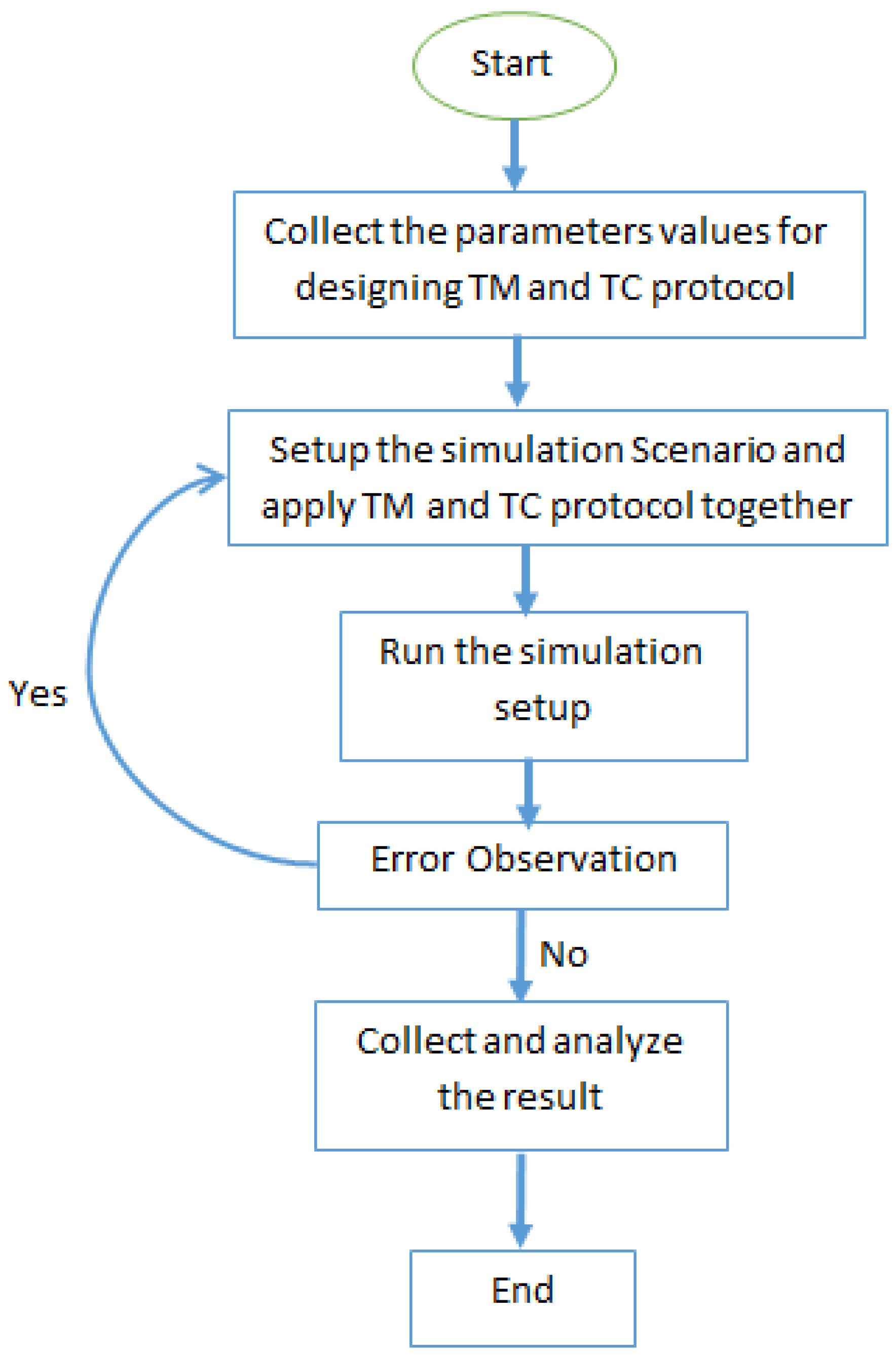
4. Simulation Results and Analysis

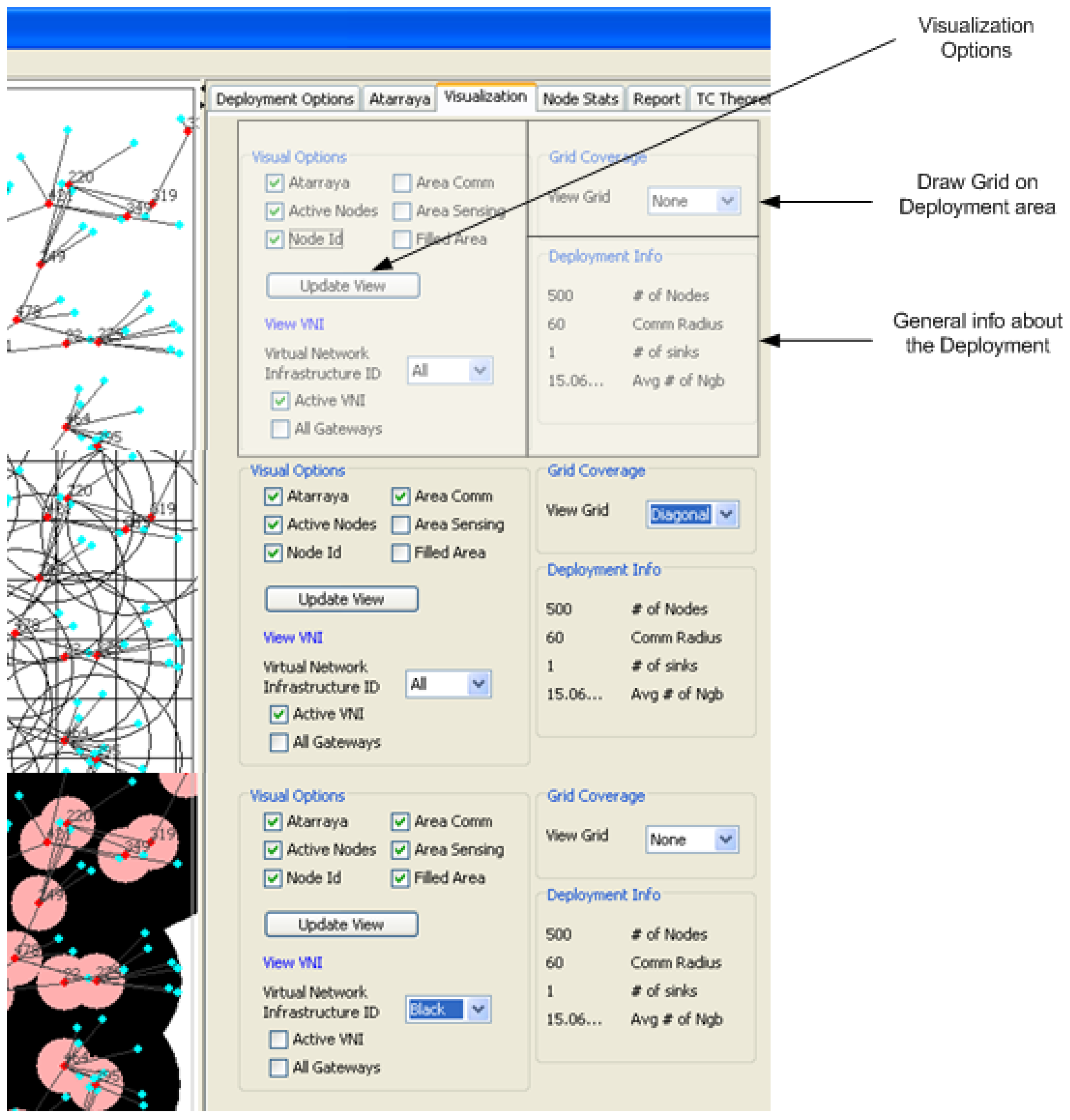
A dense topology sensor network [17] is considered as a case study. Extensive simulation work is performed using Atarraya software [51] and the performance of the proposed system analyzed. Atarraya is an even driver simulator to design, evaluation of well-known topology control algorithm to save sensor node energy in the wireless sensor network. Specifically, it was designed for testing both topology construction and maintenance protocols. Moreover, it supports a different platform for integration with graphical user interface (GUI) under free license software version GNU 3. Its also provides the opportunity to compare the various algorithm performance in a predetermined set of energy and communication environment. Figure 5 shows a sample of the topology visualization of the Atarraya simulator.

The topology maintenance protocols are simulated based on four different performance metrics: (a) the number of active nodes; (b) number of active nodes reachable from the sink; (c) area of communication coverage; and (d) area of sensing coverage. To analyze the performance of each metric, four types of well-known topology construction protocols, A3, A3 coverage (A3-Cov), Connected Domain Set based on Rule K (CDS-Rule-K) and Energy efficient connected domain set (EECDS), which are frequently used in a construction network (i.e., to connect the nodes to each other), are considered. However, after being connected, as they cannot maintain the optimum connection route to provide the optimum performance, which is the main aim, a combination of a topology construction protocol and a maintenance one can provide an optimal result for monitoring a large area such as a high-rise building. The simulation results are described in the following sections.

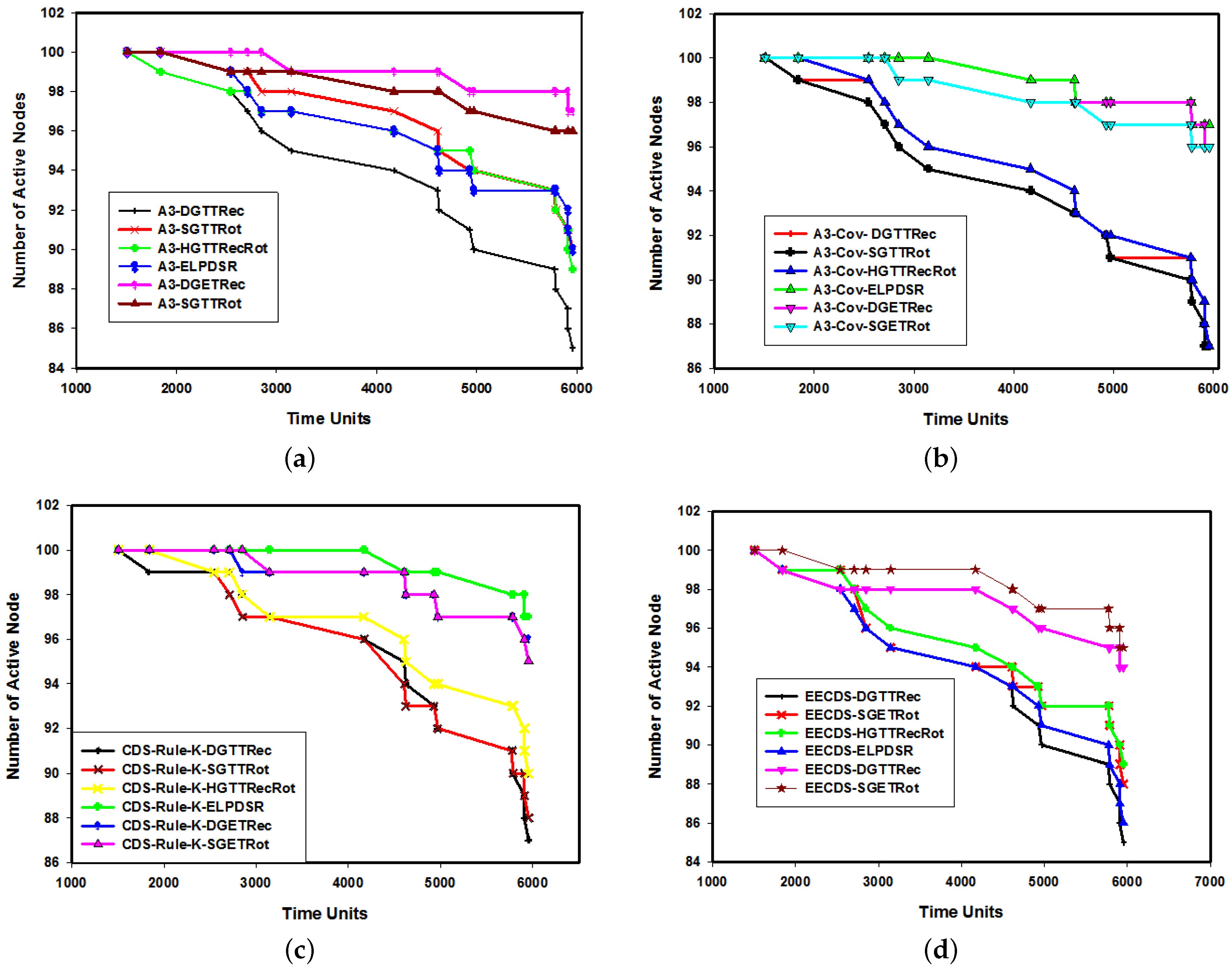
4.1. Number of Active Nodes

In this section, the experimental results obtained from the proposed model using the topology maintenance modes considered are analyzed based on the number of active nodes.

4.1.1. A3 Protocol

In this sub-section, the computational results for the topology maintenance protocol with the A3 construction one [44] are compared to find the best combination of them in terms of active nodes. To extend the lifetime of the monitoring network [38], the maintenance technique keeps the number of nodes as low as possible by maintaining the currently connected topology towards its optimal connection. Figure 6a depicts the simulation results obtained from the A3 technique using six different topology maintenance modes, the A3-DGTTRec, A3-SGTTRot, A3-HGTTRecRot, A3-ELPDSR, A3-DGTTRec and A3-SGTTRot.

It is clear that the A3-DGTTRec mode provides better results than the A3-SGTTRot, A3-HGTTRecRot, A3-ELPDSR, A3-DGTTRec and A3-SGTTRot ones while the A3-SGTTRot one produces a moderate amount of active nodes. On the other hand, the A3-DGTTRec mode obtains the highest number of active nodes which decreases a network’s lifetime due to greater consumption of the nodes’ energy. It can be seen that the A3-DGTTRec maintenance mode produces the best results because it consumes the minimum amount of energy and also always generates a dynamic version of the previous one. Moreover, it improves the lifetime of a network compared with the A3-ELPDSR one. The A3-SGTTRot mode provides a moderate system performance compared with that of the A3-DGETRec one and, initially, the A3-HGTTRecRot one gives good results which gradually deteriorate until a network time-out occurs. Overall, the A3-DGTTRec mode exhibits better results than the others and extends the lifetime of the monitoring network.

4.1.2. A3-Cov Protocol

The experimental results obtained from the proposed maintenance modes using the A3-Cov topology construction technique are compared to determine their capabilities in terms of the A3-Cov protocol. Figure 6b illustrates the computational results over the transmission period considered n which it is clear that all the modes provide gradually decreasing values over this period. Initially, all obtain 100% results which gradually decrease over the transmission period and indicate that the percentage value of the A3-Cov-SGTTRot mode is always lower than all the others considered. On the other hand, the A3-Cov-SGETRot mode demonstrates fewer changes but greater than the A3-Cov-DGTTRec, A3-Cov-SGTTRot and A3-Cov-HGTTRecRot ones. Despite some changes in the A3-Cov-ELPDSR mode, its percentage continues to decrease and obtain more active nodes over the whole period. Therefore, as the A3-Cov-SGTTRot mode provides fewer active nodes, it is more capable of reducing energy consumption than the others.

4.1.3. CDS-Rule-K Protocol

Figure 6c shows the results obtained by the proposed topology maintenance techniques using the CDS-Rule-K construction protocol. It should be noted that more active nodes consume more energy due to their generating many messages. Therefore, the experimental results show that the CDS-Rule-K-SGTTRot mode exhibits better capability while the CDS-Rule-K-DGTTRec one obtains a similar result. On the other hand, as the CDS-Rule-K-ELPDSR mode has more active nodes, it degrades the system’s performance by consuming more energy. It is clear that the performance of the CDS-Rule-K-DGTTRec mode is similar to that of the CDS-Rule-K-SGTTRot one while the CDS-Rule-K-HGTTRecRot mode shows a moderate performance and the CDS-Rule-K-SGTTRot one draws more active nodes than the CDS-Rule-K-DGTTRot one.

4.1.4. EECDS Protocol

The experimental results obtained from six different modes of a maintenance approach, namely, the DGTTRec, SGTTRec, HGTTRecRot, ELPDSR, DGETRec and SGETRot using the EECDS topology construction protocol are shown in Figure 6d. It can be seen that the EECDS-DGTTRec and EECDS-ELPDSR ones extend the life-span of the monitoring network more than the EECDS-HGTTRecRot and EECDS-SGETRot ones, and the EECDS-DGTTRec mode produces better results than the EECDS-ELPDSR one while using a dynamic version of a connected topology with information of neighbouring nodes.

4.2. Number of Nodes Reachable from Sink

This section presents the simulation results for the number of active nodes reachable from the sink.

4.2.1. A3 Protocol

In this section, the performance of the A3 maintenance protocol in the case of a node reachable from the sink is analyzed. Figure 7a is a graphical representation of the computational results in which it is illustrated that the A3-DGETRot mode extends the life-span of the monitoring system more than the A3-SGETRot, A3-SGTTRoc and A3-DGTTRoc ones while, overall, the A3-ELPDSR mode produces the optimum result.

4.2.2. A3-Cov Protocol

This section analyzes the simulation results obtained from the maintenance technique for the number of nodes reachable from the sink using the A3-Cov protocol, for which it is considered that the nodes are distributed uniformly in the 600 m×600 m monitoring area. The communication coverage area is 100 m [52] with 100 nodes using the communication coverage datasheet from Mica Z mote. This part of the simulation shows how many active nodes are reachable from the sink and how resources are used in the modes considered.

Figure 7b illustrates the simulation results for the number of nodes reachable from the sink obtained by the maintenance approach using the A3-Cov topology construction protocol. It is seen that the A3-Cov-SGTTRot mode enhances the life-span of the network more than the A3-Cov-ELPDSR and A3-Cov-DGTTRec ones and its performance is similar to that of the A3-Cov-DGTTRec one. In addition, the A3-Cov-HGTTRecRot and A3-Cov-DGTTRec modes show similar improved results. This is expected because the A3-Cov-HGTTRecRot mode can create a global version of the connected domain set by adding or removing nodes to obtain a better approximation of the optimal one and exhibits a better life-span of the monitoring network.

4.2.3. CDS-Rule-K Protocol

Figure 7c depicts the computational performances of the proposed CDS-Rule-K maintenance protocol over the transmission time, showing that the CDS-Rule-K-HGTTRecRot mode has a better response than the others while consuming less of the nodes’ energy and preserving the network’s connectivity and other properties. In addition, the CDS-Rule-K-DGTTRec and CDS-Rule-K-SGTTRot modes save moderate amounts of the nodes’ energy. Therefore, it can be concluded that the CDS-Rule-K-HGTTRecRot mode is a good choice for saving the nodes’ energy.

4.2.4. EECDS Protocol

The main goal of this case study is to analyze the number of nodes reachable from the sink using the EECDS topology construction protocol. The overall results obtained from the simulation model are depicted in Figure 7d which shows that the EECDS-DGTTRec maintenance mode proves a good candidate. Before 3000 time units, the EECDS-HGTTRecRot mode produces almost similar results to the EECDS-DGTTRec one and then exhibits better ones until a transmission time-out occurs. Between 5000 and 6000-time units, EECDS-DGETRot and EECDS-DGTTRec modes provide approximately similar results. The performances of the EECDS-HGTTRecRot and EECDS-DGTTRec modes continue to be very close, with the latter improving the lifetime of the monitoring system while others degrade its performance. Overall, it can be seen that the EECDS-DGTTRec mode extends the network’s lifetime more than all the other modes considered.

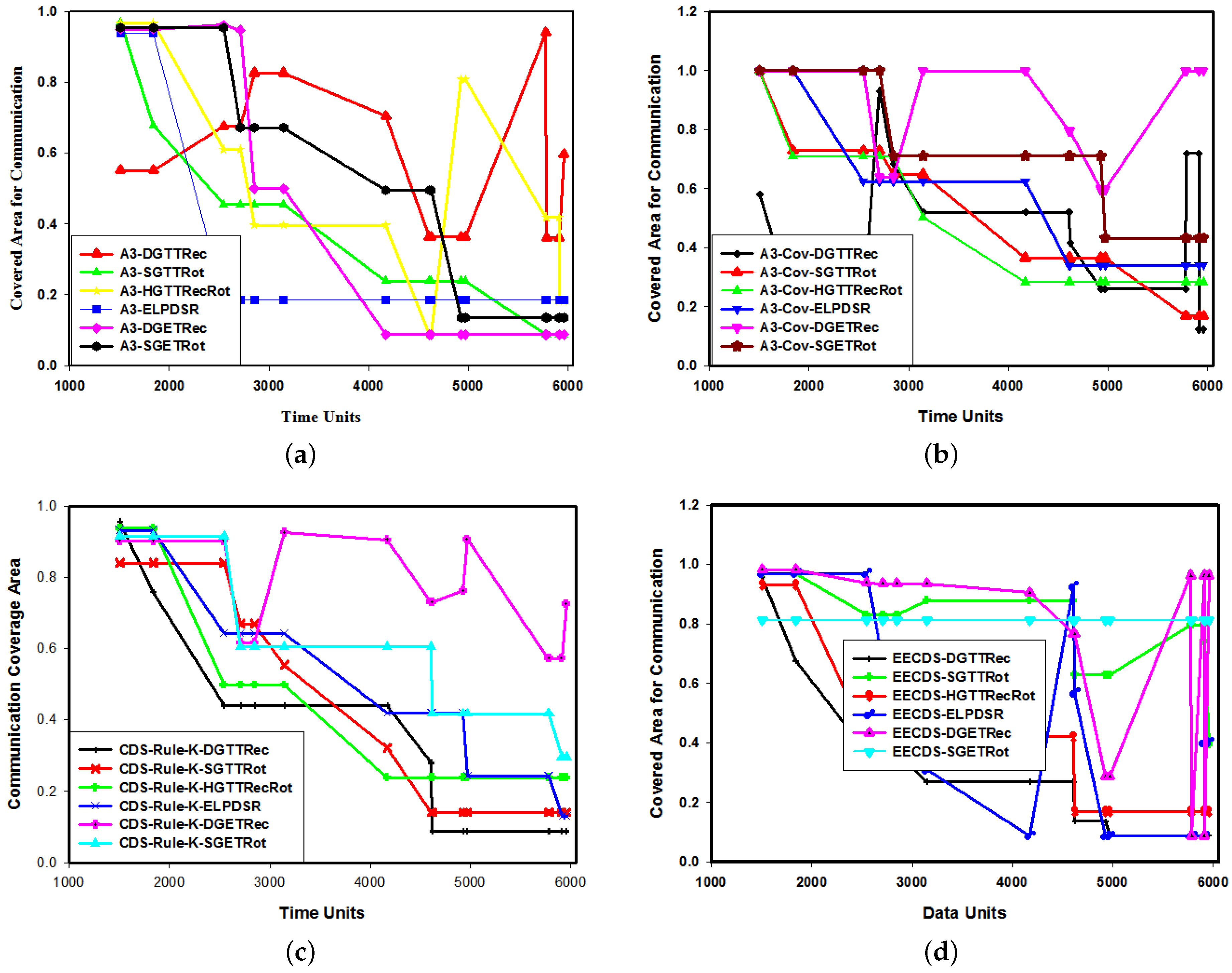
4.3. Area of Communication Coverage

This section describes the results in terms of the area of communication coverage using the proposed maintenance modes.

4.3.1. A3 Protocol

As the area of communication coverage determines that of the monitoring network, it is expected that it should be as large as possible. Figure 8a shows the simulation results for that area using the proposed modes which indicate that the A3-DGETRec one increases the coverage distance and life-span of the monitoring network while the A3-SGTTRot one provides very similar results until 3000 time units. From 3000 to 6000 time units, the A3-DGTTRec mode provides a greater communication coverage area and, compared with it, the A3-SGETRot and A3-HGTTRecRot ones degrade the system’s performance. Overall, the A3-DGTTRec maintenance mode obtains the best results.

4.3.2. A3-Cov Protocol

In this experimental analysis, the simulation results obtained from the maintenance modes using the A3-Cov construction protocol for the communication coverage area are compared. For a large-area monitoring network, the system needs to cover a larger area. Figure 8b shows that the A3-Cov-SGETRot mode proves itself a good candidate, as does the A3-Cov-DGETRec one. On the other hand, between 2000 and 5000 time units, the A3-Cov-DGETRec mode provides the maximum coverage area of all the others and then, after 5000 time units, the A3-Cov-DGTTRec one again covers the greatest communication area for monitoring structural health data.

4.3.3. CDS-Rule-K Protocol

Figure 8c illustrates the simulation results for the maintenance modes in terms of the communication coverage area using the CDS-Rule-K protocol. The CDS-Rule-K-DGETRot mode depicts the largest communication coverage area of between 100 and 3000 time units while that of the CDS-Rule-K-DGETRot one is similar and, after 3000 to 6000 time units, is capable of achieving the highest amount of communication coverage area. The main objective of this case study is to determine the optimum combination mode for saving the nodes’ energy and extending the communication coverage area of a WSN by connecting the minimum number of nodes required to provide a large sensing area. In terms of the topology maintenance protocols, the results show that the CDS-Rule-K-DGETRot mode exhibits the largest communication coverage area compared with those of the CDS-Rule-K-DGTTRec, CDS-Rule-K-SGTTRot, CDS-Rule-K-HGTTRecRot, CDS-Rule-K-ELPDSR and CDS-Rule-K-SGETRot modes.

4.3.4. EECDS Protocol

The communication coverage areas of the proposed maintenance protocols obtained by six different modes of the EECDS construction protocol between 1000 and 6000 time units are illustrated in Figure 8d. For more than 5000 time units, the areas provided by the EECDS-ELPDSR and EECDS-HGTTRecRot modes decrease dramatically while the performances of the EECDS-DGETRec and EECDS-SGTTRec ones are moderately changed. The EECDS-DGETRec mode provides the largest coverage area over the entire transmission period and both the EECDS-DGTTRec and EECDS-HGTTRecRot ones the smallest. The sizes of their communication coverage areas exponentially decrease in the cases of the EECDS-ELPDSR, EECDS-HGTTRecRot and EECDS-DGTTRec modes at approximately 4000 time units after which the EECDS-ELPDSR one has the largest coverage area for a short period of units while the performances of the other two continue to decrease. It can be concluded that the most popular mode of the EECDS construction protocol is the EECDS-DGETRec one.

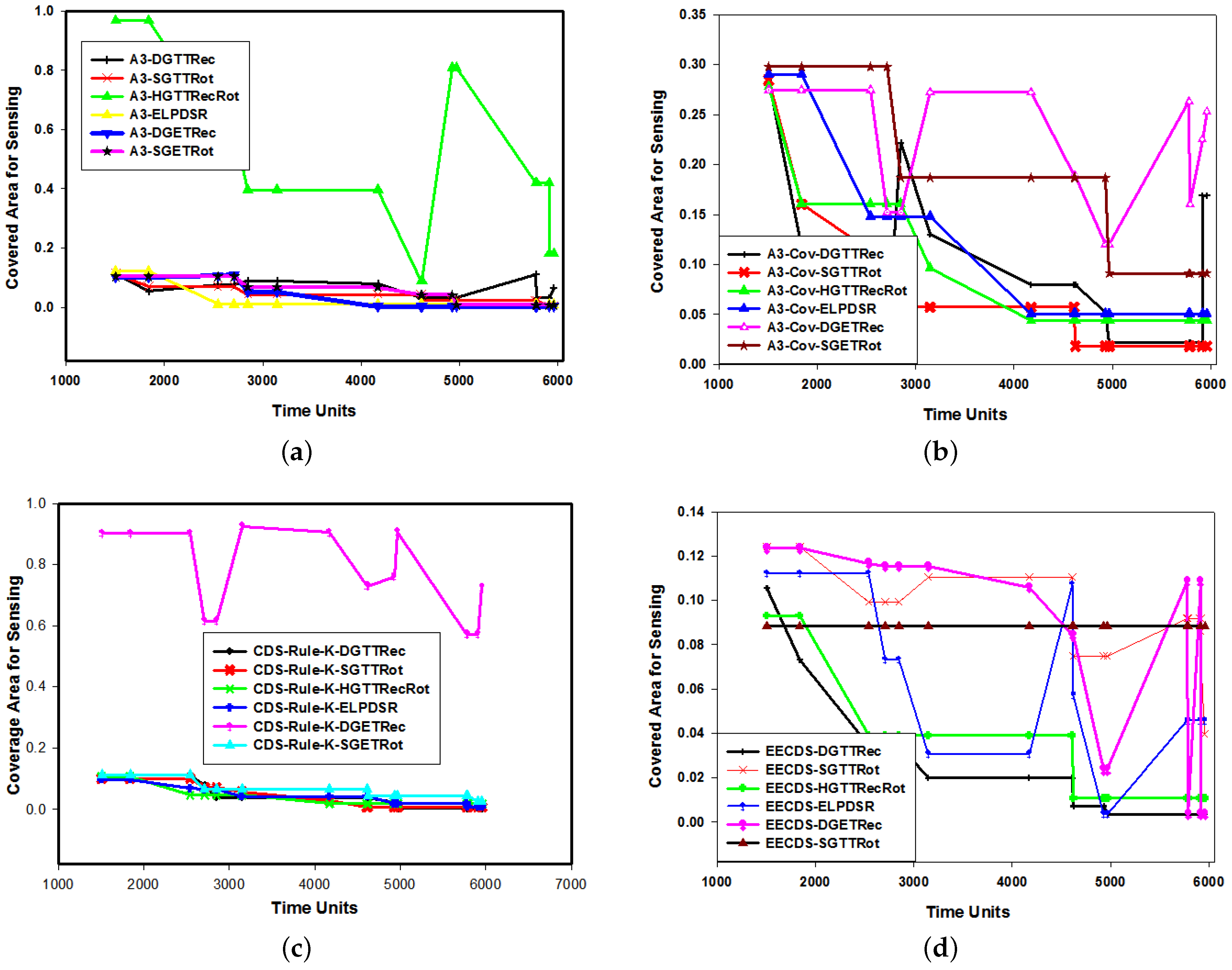
4.4. Area of Sensing Coverage

The main objective of this section is to analyze the sensing capability of the proposed model. The total number of participating active nodes determine the sensing capability of the network and, to cover the deployment area for monitoring structural health, the sensing coverage area should be equal or larger. In this section, the simulation results for this area using different maintenance modes are discussed.

4.4.1. A3 Protocol

The simulation results for the sensing coverage area of the proposed modes considered using the A3 topology construction protocol between 1000 and 6000 time units are shown in Figure 9a. The sensing coverage area of the A3-HGTTRecRot mode decreases dramatically at approximately 4800 time units and then increases until 5000 before decreasing gradually again but declines most of the time during a short period of increasing values. Over the whole life-span, this mode provides a better result than all the other as it provides the highest sensing coverage area while the A3-DGETRec mode produces the lowest for the A3-based sensing coverage measurement.

4.4.2. A3-Cov Protocol

Figure 9b shows the sensing coverage areas of six different maintenance modes considering the A3-Cov topology construction protocol. Through 5000 time units, these areas obtained by the A3-Cov-ELPDSR, A3-Cov-HGTTRecRot and A3-Cov-SGTTRot modes decrease exponentially until a transmission time-out occurs. While that of the A3-Cov-SGETRot mode decreases moderately like a step function, the A3-Cov-DGETRec one produces better sensing coverage through its gradually increasing and decreasing values, which mainly increase during a small period of decreasing values, than all the other modes.

4.4.3. CDS-Rule-K Protocol

The computational results obtained from the maintenance modes in terms of the performance metrics for the sensing coverage area using the CDS-Rule-K construction protocol are presented. Figure 9c shows these areas of six different modes of the CDS-Rule-K maintenance protocol. Over the entire period of the transmission network, that of the CDS-Rule-K-HGTTRecRot mode exhibits a constant value until 2500 time units and then dramatically decreases until 3000. After this, it increases again until approximately 4200 time units and then, through random fluctuations, reaches approximately 80% of the sensing coverage area while the areas computed by the CDS-Rule-K-DGETRec, CDS-Rule-K-SGTTRot, CDS-Rule-K-ELPDSR, CDS-Rule-K-DGETRec and CDS-Rule-K-SGETRot modes gradually decrease to about 10%, with that of the CDS-Rule-K-DGETRec mode always significantly higher than those of the others.

4.4.4. EECDS Protocol

Figure 9d shows the simulation results for the sensing coverage areas of the proposed modes using the EECDS topology construction protocol. Those of the EECDS-HGTTRecRot and EECDS-DGTTRec modes decrease dramatically until a transmission time-out occurs, that of the EECDS-SGTTRot one remains constant at 8.44%, that of the EECDS-DGETRot one decreases gradually until 5000 time units and then fluctuates randomly before the network fails, that of the EECDS-ELPDSR one decreases as a step function until approximately 3200 time units before reaching its peak value again. Considering the transmission time units, the EECDS-DGETRec mode produces a better coverage area than all the others and, over the entire transmission period, has the highest sensing coverage area while the EECDS-DGTTRec one has the lowest.

4.5. Comparative Analysis

In this section, the best results of each case study are compared and presented in terms of the previously considered four performance metrics. To reduce the energy consumption of WSNs, a proper node deployment scheme has to be selected as the density of its nodes determine the life-span of a network. Therefore, to extend the monitoring system’s lifetime, this density must be scalable with the monitoring area. From the results, the best topology maintenance mode is investigated.

Table 5. Comparison of performances in terms of numbers of active and sink-reachable nodes.

Parameter	Maintenance Protocol	Transmission Time (s)
		1507	3146	4621	5777	5956
Number of Active Nodes	A3-DGETRec	100	98	95	93	90
	A3-Cov-SGTTRot	100	95	93	90	87
	CDS-Rule-K-ELPDSR	100	97	93	91	87
	EECDS-SGETRot	100	95	92	89	85
Sink-reachable Nodes	A3-ELPDSR	35	3	3	3	3
	A3-Cov-HGTTRecRot	85	13	13	13	13
	CDS-Rule-HGTTRecRot	30	13	13	5	5
	EECDS-DGTTRec	30	6	2	1	1

shows a comparison of the results obtained from each topology construction protocol with the maintenance mode for the numbers of active and sink-reachable nodes. It can be seen that the EECDS-SGETRot mode has the most active nodes (85) compared with the A3-Cov-SGTTRot one. In terms of the number of active nodes reachable from the sink, it can be seen that the EECDS-DGTTRec mode exhibits a better result than all the others due to it consuming less energy to reach an efficient number of nodes. In the case of the active nodes, the EECDS-SGTTRec mode provides the optimum number of reachable ones.

Table 6. Comparison of performances in terms of communication and sensing coverage areas.

Parameter	Maintenance Approach	Transmission Period (s)
		1507	3146	4621	5777	5956
Communication Coverage Area	A3-DGETRec	0.551	0.826	0.363	0.940	0.896
	A3-Cov-DGETRec	0.999	0.999	0.795	0.998	0.998
	CDS-Rule-K-DGETRec	0.902	0.925	0.729	0.572	0.724
	EECDS-DGETRec	0.983	0.935	0.766	0.963	0.964
Sensing Coverage Area	A3-HGTTRecRot	0.967	0.936	0.088	0.419	0.181
	A3-Cov-DGETRec	0.274	0.272	0.189	0.263	0.253
	CDS-Rule-K-DGETRec	0.902	0.925	0.729	0.572	0.724
	EECDS-DGETRec	0.123	0.115	0.084	0.108	0.003

shows a comparison of the best topology maintenance mode in terms of the communication and sensing coverage areas. The simulation results reveal that the A3-Cov-DGETRec maintenance mode has more communication coverage than the others. For the sensing coverage area, the proposed CDS-Rule-K-DGETRec mode has the highest which is better than that of the A3-HGTTRecRot one. This can be explained by the fact that a higher sensing coverage area leads to better sensing of a large area.

5. Conclusions

In this research work, an IoT-based WSN for SHM is proposed. The topology maintenance protocol provides the maintenance version of a constructed topology for creating a new and efficient one for monitoring all types of structural health. Our proposed method is suitable for measure vibration or seismic event. In such cases sensing and communication performance metric were chosen as system performance measurement parameters. The simulation results reveal that, for a number of active nodes, the EECDS-SGETRot mode exhibits the optimum result for achieving a better version of a monitoring network and, for sink-reachable nodes, the EECDS-DGTTRec one is considered the best. As the A3-Cov-DGETRec maintenance mode extends the lifetime of a monitoring network, it is a potential candidate for a/monitoring system. In addition, the CDS-Rule-K-DGETRec one increases the lifetime of a monitoring system by prioritizing the sensing area.