Article

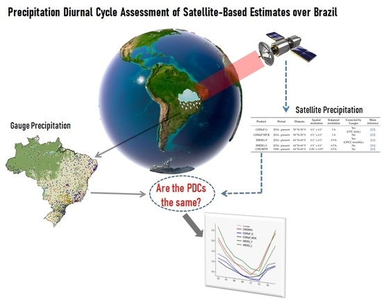
Precipitation Diurnal Cycle Assessment of Satellite-Based Estimates over Brazil

by
João Maria de Sousa Afonso
1,*,
Daniel Alejandro Vila
1,
Manoel Alonso Gan
1,
David Pareja Quispe
1,
Naurinete de Jesus da Costa Barreto
1,
Joao Henry Huamán Chinchay
2 and
Rayana Santos Araujo Palharini
1
1
National Institute for Space Research, São José dos Campos 12227-010, Brazil
2
Servicio Nacional de Meteorología e Hidrología del Perú, 11076 Lima, Peru
*
Author to whom correspondence should be addressed.
Remote Sens. 2020, 12(14), 2339; https://doi.org/10.3390/rs12142339
Submission received: 22 June 2020 / Revised: 14 July 2020 / Accepted: 15 July 2020 / Published: 21 July 2020

Abstract

:
The main objective of this study is to assess the ability of several high-resolution satellite-based precipitation estimates to represent the Precipitation Diurnal Cycle (PDC) over Brazil during the 2014–2018 period, after the launch of the Global Precipitation Measurement satellite (GPM). The selected algorithms are the Global Satellite Mapping of Precipitation (GSMaP), The Integrated Multi-satellitE Retrievals for GPM (IMERG) and Climate Prediction Center (CPC) MORPHing technique (CMORPH). Hourly rain gauge data from different national and regional networks were used as the reference dataset after going through rigid quality control tests. All datasets were interpolated to a common 0.1° × 0.1° grid every 3 h for comparison. After a hierarchical cluster analysis, seven regions with different PDC characteristics (amplitude and phase) were selected for this study. The main results of this research could be summarized as follow: (i) Those regions where thermal heating produce deep convective clouds, the PDC is better represented by all algorithms (in term of amplitude and phase) than those regions driven by shallow convection or low-level circulation; (ii) the GSMaP suite (GSMaP-Gauge (G) and GSMaP-Motion Vector Kalman (MVK)), in general terms, outperforms the rest of the algorithms with lower bias and less dispersion. In this case, the gauge-adjusted version improves the satellite-only retrievals of the same algorithm suggesting that daily gauge-analysis is useful to reduce the bias in a sub-daily scale; (iii) IMERG suite (IMERG-Late (L) and IMERG-Final (F)) overestimates rainfall for almost all times and all the regions, while the satellite-only version provide better results than the final version; (iv) CMORPH has the better performance for a transitional regime between a coastal land-sea breeze and a continental amazonian regime. Further research should be performed to understand how shallow clouds processes and convective/stratiform classification is performed in each algorithm to improve the representativity of diurnal cycle.

Graphical Abstract

1. Introduction

Precipitation, and its time and space distributions, is of paramount importance to any country, in particular for those of continental size such as Brazil. Indeed, rain gauge data are always required in almost all areas of activities: water resources management (with emphasis on potable water), agriculture, energy generation by hydroelectric power plants, just to mention some. Reliable planning for the operation and maintenance of these activities requires consistent and accurate data [1]. On the other hand, the largest part of Amazon rain forest, which is located over Brazilian territory, plays an important role in the global precipitation and energy budgets [2].
However, the meteorological and climate multi-scale processes (mainly at the highest spatial and temporal scales) over these unpopulated regions have not been well understood, due to the absence or a poor distribution of surface measurements, especially, in complex terrain and remote forest areas. Satellite-based precipitation estimates (SPE) could be an excellent complement to conventional data in those regions where other measurement systems are difficult to implement and maintain [3], but they need to be validated, in most cases regionally, to understand the uncertainties associated with the physical processes associated with each rainfall regime.
The characterization of the Precipitation Diurnal Cycle (PDC), and how it is related with thermodynamic processes in a given region, is a key factor to understand the rainfall variability in continental regions [4]. In such a case, high spatial and temporal sampling is important to understand the meteorological processes associated with the PDC. The newer versions of SPEs have a spatial resolution around 10 km and a temporal resolution of 30 min to one hour, which allows to use those retrievals to get a good representation of the PDC [5]. However, it is necessary to assess the robustness of the various satellite-based precipitation products in order to assess uncertainties associated with those retrievals [6,7].
Since 27 November 1997 the Tropical Rainfall Measuring Mission (TRMM) and the TRMM Mutisatellite Precipitation Analysis (TMPA) product, which combines frequent infrared (IR) sampling, precipitation estimations from active and passive microwave observations (AMW + PMW), and rain gauge data, have been provided near-global precipitation maps with different temporal and spatial resolutions. Those retrieval were extensively used to study energy and water cycles over the tropics, including PDC, in different regions of the world [8,9]. Pioneering studies in Brazil using the TRMM products were carried out by Mota et al. [10] from December 1997 to November 2000 and they reported that the rain data derived from the passive microwave of the TRMM Microwave Imager (TMI) are more consistent with the in-situ observations of the PDC, when compared with the estimated data derived from models such as Global Precipitation Climatology Project (GPCP), radar estimates of the Precipitation Radar (PR) and IR channel of the GOES Precipitation Index (GPI).
Another important study worth mentioning was carried out by Brito et al. [11] which characterized in detail different PDC regimes over the continent and adjacent oceanic areas in northern Brazil during the southern fall (rainy season) for the period 1998-2010 using TRMM products. More recently, Giles et al. [12] pointed out the different characteristics of sub-daily precipitation regimes in South America, the issues with conventional climate models and the uncertainty in satellite products and reanalyses.
The Global Precipitation Measurement (GPM) mission was launched on 28 February 2014, with an advanced dual-frequency precipitation radar (DPR) with Ka and Ku band (35.5 and 13.6 GHz, respectively) and the GPM microwave imager (GMI) with multi-frequency between 10–183 GHz [13] in replacement of the successful TRMM satellite. The GPM constellation, which includes data from several satellites, enables space agencies around the world to develop advanced techniques for generating products with better temporal and spatial sampling and coverage rainfall observations [14]. The high spatial and temporal resolution of this new generation of products create new challenges for the scientific community. There are some studies in Brazil to evaluate this new generation of products, mainly on a daily scale. For example, Rozante et al. [1] compared different algorithms developed by Japan Aerospace Exploration Agency (JAXA) and the National Aeronautics and Space Administration (NASA) and concluded that all products are capable to reproduce, with an acceptable degree of precision, different precipitation patterns over Brazilian territory.
The main objective of this study is to assess the ability of several high-resolution satellite-based precipitation estimates to represent the PDC over Brazil during the 2014–2018 period, after the launch of the Global Precipitation Measurement satellite (GPM). The selected algorithms are: The Global Satellite Mapping of Precipitation (GSMaP) from JAXA; the Climate Prediction Center (CPC) MORPHing technique (CMORPH) from CPC/NOAA and The Integrated Multi-satelliE Retrievals for GPM (IMERG) from NASA. This article is organized as follows: Section 2 presents information from the study area while the data sets and statistics are presented in Section 3. Section 4 presents the main results of this research and discussion. The conclusions are provided in Section 5.

2. Study Area and Data

2.1. Study Area

Brazil covers 8,515,759 km2 area in South America territorial which is approximately the domain of 37°S–8°N and 35°–73°W as shown in Figure 1. Due to its continental dimensions, it presents a great diversity of landscapes, topography, biodiversity and climates, as well as different precipitation regimes [1].
The different precipitation regimes in Brazil are mainly associated with large-scale systems acting according to seasonality, the most important being the South Atlantic Convergence Zone (SACZ) that acts in the southern summer ranging from the southeast of the country to the far west Amazonian region; the Intertropical Convergence Zone (ITCZ) acts mainly in the fall over the north and northeast regions and transient systems (baroclinic systems) acting mainly in the winter over most parts of Brazil. A complete description of these precipitation regimes can be found in [15].

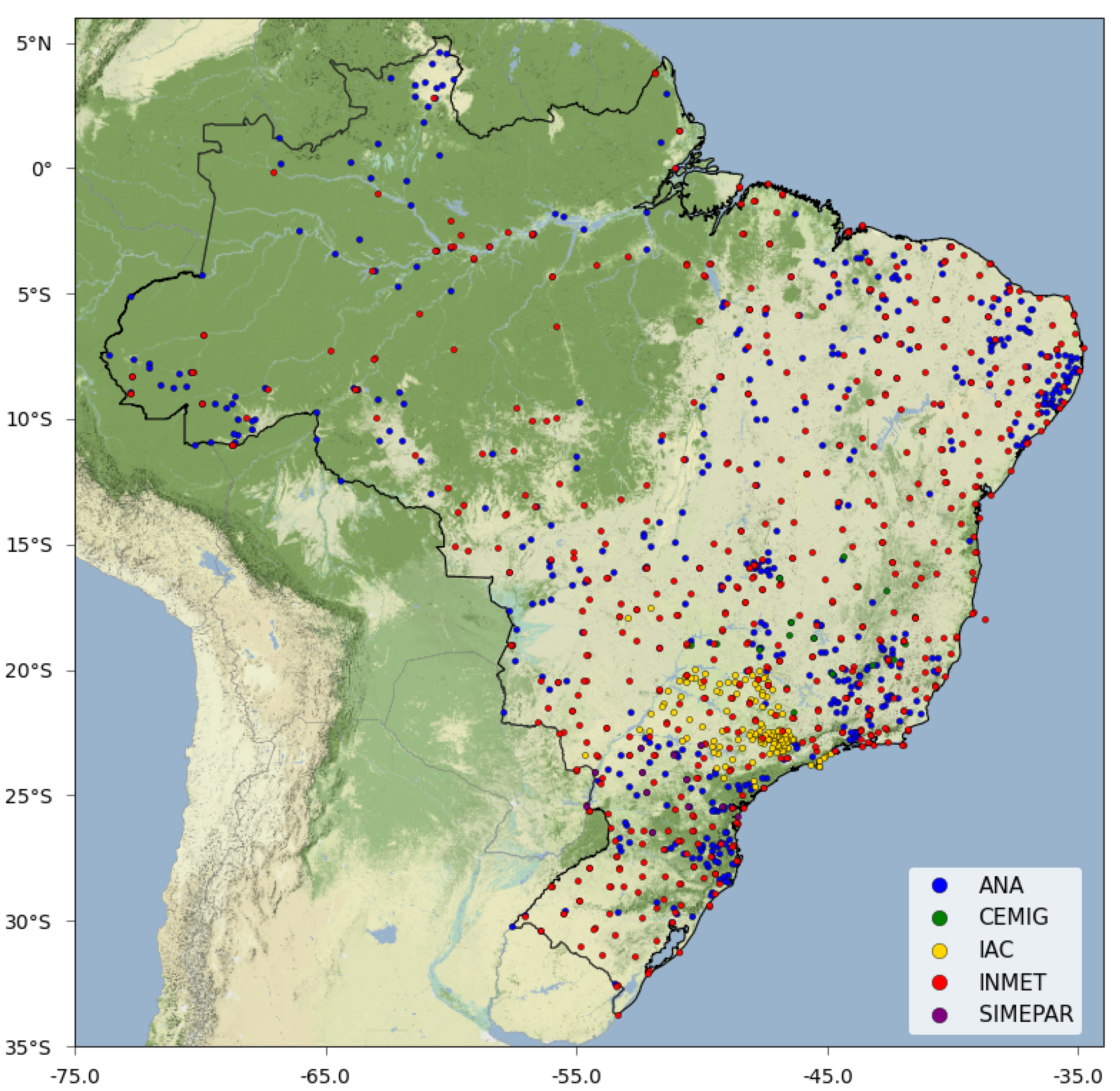
2.2. Ground Gauge and Quality Control

The present study covers the period from 2014–2018. The initial date was chosen due to the availability of products derived from NASA’s GPM measurements. During this period, hourly precipitation data were obtained from rain gauge networks from Brazilian National Institute of Meteorology (INMET; http://www.inmet.gov.br), the National Water Agency (ANA; www.ana.gov.br), Companhia Energética de Minas Gerais (CEMIG; http://www.cemig.com.br), Agronomic Institute (IAC; http://www.iac.sp.gov.br/) and Sistema Meteorológico do Paraná (SIMEPAR; http://www.simepar.br/). All precipitation data are stored the National Institute for Space Research (INPE; https://www.cptec.inpe.br/ database in Brazil. Table 1 presents the detailed information about the aforementioned networks.
The rain gauge data used in this study cover different periods and their metadata (sources, space coverage, time resolution and number) are summarized in Table 1. Hourly and tri-hourly precipitation studies, especially those involving the diurnal cycle, are not so frequent due to their low reliability and quality. Therefore, a quality control (QC) procedure is essential; the schematic flow diagram of this processes is given in Figure 2a, while the space distribution and percentage of available reference data (after QC test and gridding procedure) is shown in Figure 2b. A concise description of the quality control procedures used in this study is given below:
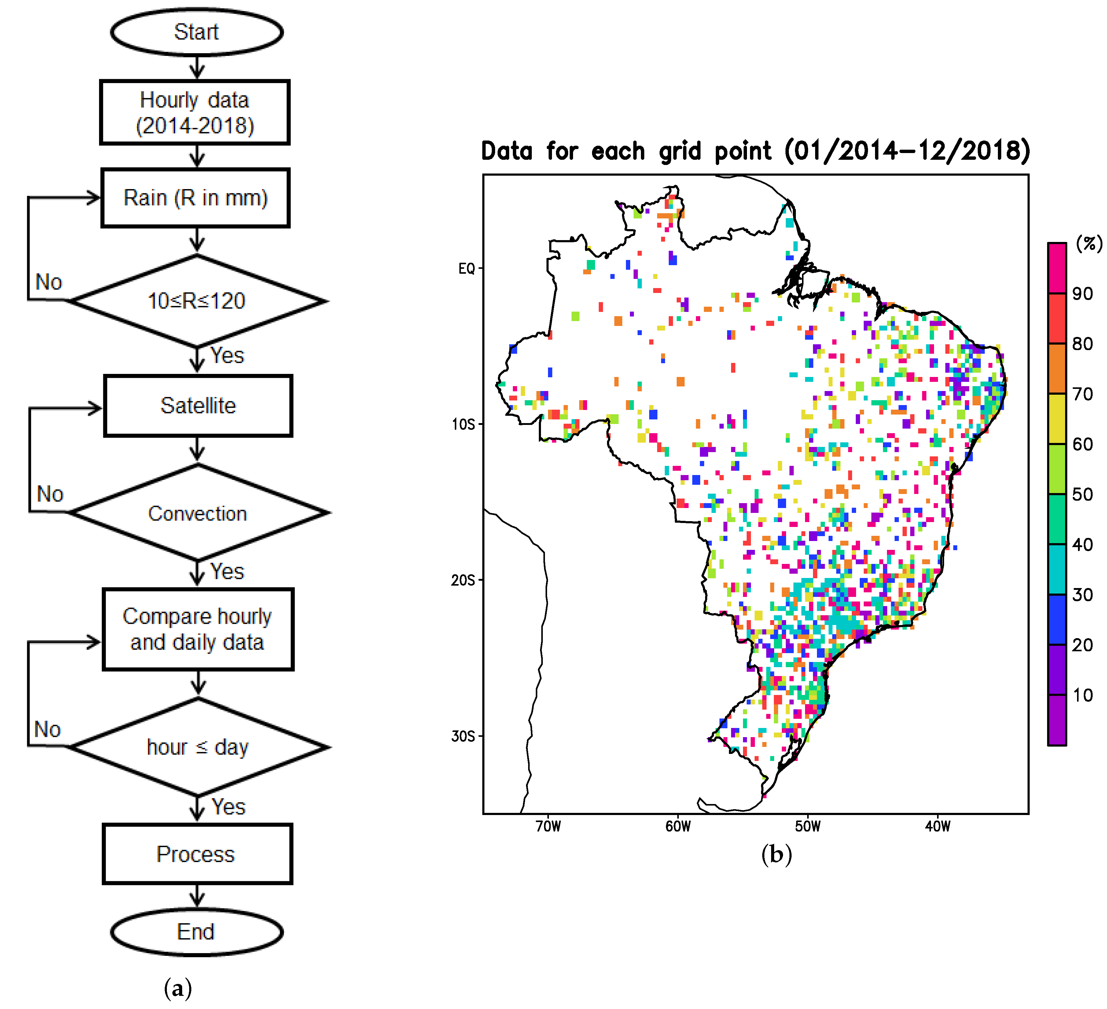
  • Missing and unrealistic values were detected from the reference dataset. In some cases like INMET, CEMIG and SIMEPAR data are flagged as 9999.99 while the other networks use a spurious value (i.e., 650 mmh−1);
  • A threshold between 10 mmh−1 and 120 mmh−1 was established for convective rainfall (also adopted at SIMEPAR) to apply specific quality control tests, according to [16];
  • For rainfall rates within this interval, the physical characteristics of the convective clouds were compared with the correspondent satellite imagery [17] using different channels (mainly infrared and visible, when available) from GOES 13 and 16. This imagery was provided by the Satellite Division and Environmental Systems DSA/INPE;
  • The reference dataset, with different time resolution, were accumulated for three hour periods following the WMO guidelines (i.e., 00-03 UTC; 03-06 UTC; and so on);
  • Daily values (12:00-12:00 UTC) were compared with accumulated values from the previous step at each station to satisfy INPE’s quality control tests [1].
Based on the above criteria, some data were eliminated when they are missing (1) or when the cloudiness at the coordinates of the gauges did not correspond to the convection in the GOES images (3) or, even when the daily rainfall value does not match with the tri-hourly accumulation for the respective day (5). The station was totally discarded if the percentage of failures exceeded 5%.
Once the first set of tests are applied to validate the intense precipitations events, all precipitation values were analyzed (including those inferior to 10 mmh−1) using statistical techniques [18] as quantile methods and frequency distribution of rain thresholds. At the end of the process, 1261 stations were selected for the next step according to the following institutional distribution: INMET—592 stations, ANA—499 stations, CEMIG—21 stations, IAC—128 stations and SIMEPAR—21 stations (Figure 1).
The data were interpolated to a 0.1° × 0.1° uniform grid using the simple average for the rain gauges station available at each grid point (Figure 2b). Grid points where there are not rain gauges nearby were removed from the series. This approach allows, on one hand, to make the best use of the available information and, on the other hand, to make a fair comparison with the SPE values. Figure 2b shows a reasonable space distribution of the rain gauge-based precipitation data which is suitable for the purpose of this study.
The sampling frequency of data availability is quite uneven along the country with relatively low values (less than 40% of the total series) for some points in southeastern and southern Brazil due to the short period of the observations at the IAC and SIMEPAR stations while IMNET station shows a better record of accepted observations after the QC procedure (Figure 2b and Table 1).

2.3. Satellite-Based Precipitation Estimates (SPE)

High temporal and spatial resolution (almost on a global scale) of satellite-based precipitation estimates were used in this study. The products are precipitation estimates obtained from a constellation of polar and equatorial (low orbit) with on-board passive and active microwave sensors, adjusted using DPR radar data from the GPM satellite. These products are generated by morphing algorithms [19] which use geostationary IR data to attain high temporal (using cloud motion vectors) and high space resolution (Kalman filter applied to low resolution precipitation rate data [20]). The utilized algorithms are: (1) Global Satellite Mapping of Precipitation (GSMaP) from JAXA (http://sharaku.eorc.jaxa.jp/GSMaP/), that uses scattering algorithms with polarization corrected temperatures (PCTs) at 85.5 and 37 GHz; PCT85 recommended for light (stratiform) rainfall and PCT37 for heavier (convective) precipitation [21]; (2) Integrated Multi-SatellitE Retrievals for GPM (IMERG) NASA (http://pmm.nasa.gov/data-access/downloads/gpm) and (3) Morphing Technique (CMORPH) developed by the CPC/NCEP/NOAA (ftp://ftp.cpc.ncep.noaa.gov). Basically, the algorithms CMORPH and IMERG use the Goddard Profiling Algorithm (GPROF) to calculate the rainfall rates of instant showers [22] and the algorithm due to [23] for the sounder estimates (cross-track). The main characteristics of these algorithms are given in Table 2.
Some of these satellite-based precipitation estimates use gauge data with the purpose of correcting the bias of these estimates [6]. In the case of the GSMaP suite, the product GSMaP-Gauge (hereby referred to as GSMaP-G) [25] adjusts the version GSMaP-Motion Vector Kalman (MVK) with daily data from the global pluviometric analysis from NOAA CPC Unified Gauge-Based Analysis of Global Daily Precipitation. In the case of the final version of IMERG (IMERG-F) the product is generated from the version IMERG-Late with monthly data from the Global Precipitation Climatology Center (GPCC)/Deutscher Wetterdienst (DWD). The CMORPH product was used only in the non adjusted version (hereinafter referred to as CMORPH). The basic information of the above mentioned products are given in Table 2.

3. Methodology

3.1. Data Standardization

Data from all sources were classified according to the seasons: the southern summer (DJF), fall (MAM), winter (JJA) and spring (SON), for a 5-year period from 2014 to 2018. Gauge data were interpolated into a 0.1° × 0.1° uniform grid (as seen in Section 2.2) and used as reference for comparisons against the estimated values obtained from SPE’s.
The IMERG (IMERG-F and IMERG-L) and GSMaP (GSMaP-G and GSMaP-MVK) products are also available for a grid with the same resolution above, but CMORPH data are given in an irregular grid of 0.08° × 0.07° (Table 2). However, in order to facilitate the evaluation and inter comparison among the different databases, the latter were interpolated for this resolution using a bi-linear interpolation method. All the products were accumulated for three hour period (just as we did for the gauge data) according to WMO guidelines.
Interpolated gauge data were also used to mask and filter out non-valid grid points from the SPE’s in order to allow a direct comparison between the reference and estimated value at each grid point using statistical indices that will be presented in the next section.

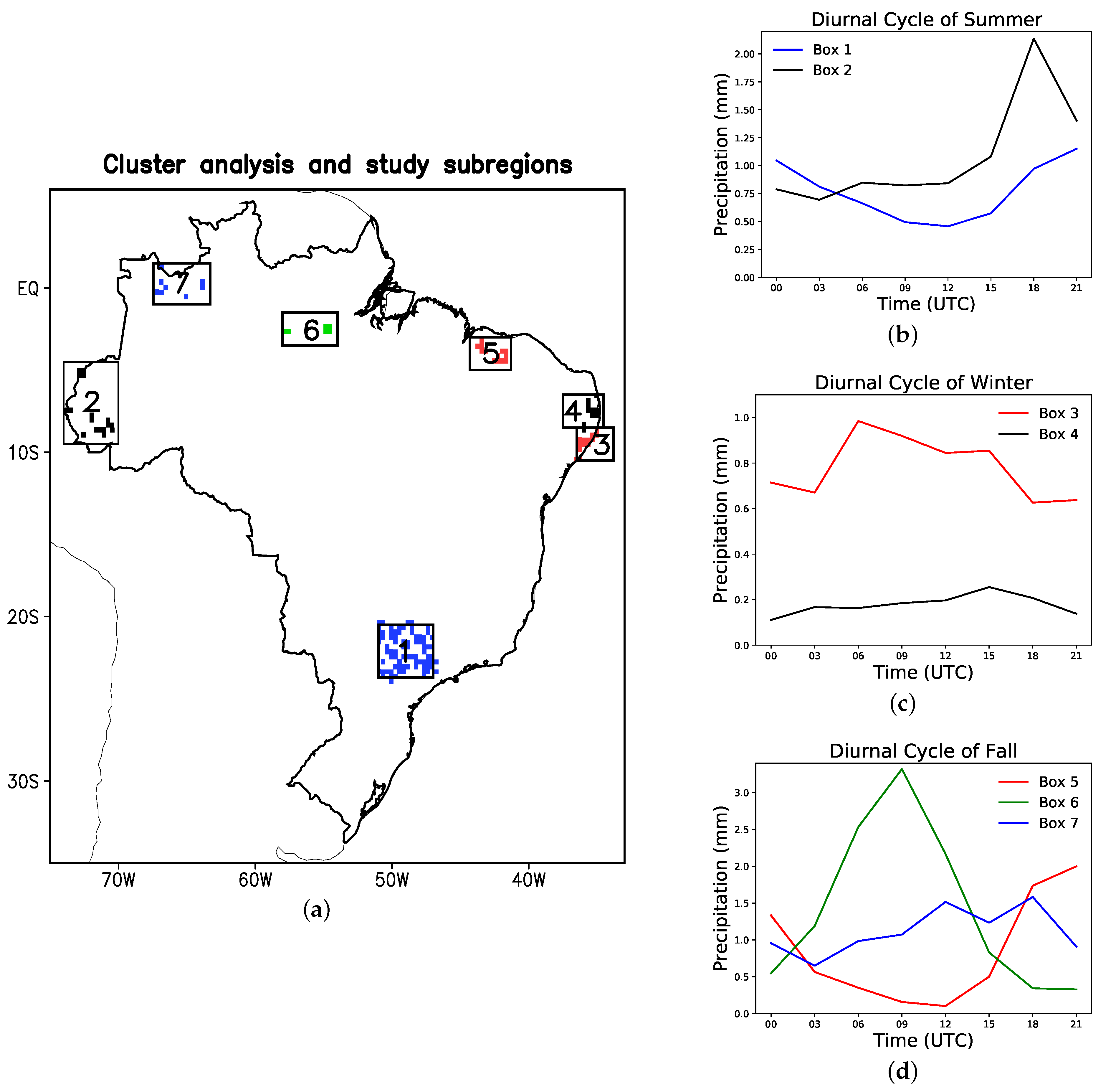
3.2. Cluster Analysis

A hierarchical Cluster Analysis technique [26] was used to determine sub regions, hereafter denominated boxes, with homogeneous PDC. The PDC is characterized by the amplitude and phase. The cluster analysis was performed on each valid grid point in the database for the 5-year period. Those valid grid points as shown in Figure 2b.
After performing that cluster analysis, seven boxes with different characteristics of the PDC were selected for this study (Figure 3b–d) for different rainy seasons.
In order to verify the rainy period for each selected box, INMET climatological data were used as shown in Figure 4. Table 3 specifies the domain, season (which coincides with the rainy period of this box) and the number of grid points for each box. The number of points considered to perform the statistical analyses are closely related to the number of available points in a given box.
As mentioned before, the cluster analysis selected seven different groups with different PDC characteristics. In the next paragraphs, will be described the main characteristics of each PDC and the main meteorological systems acting on those regions.
The largest precipitation accumulation in boxes 1 and 2 occurs during the Southern Hemisphere summer (308.46 mm and 290.30 mm, respectively) and they are modulated by the presence of the South Atlantic Convergence Zone (SACZ) which extends from western Amazonia to the Atlantic ocean [27,28,29] and to the surface radiative heating.
The box 1, which is located in the southeastern region of Brazil, is characterized with a mean maximum intensity of 1.25 mm/3 h at 2100 UTC (1800 Local Time—LT) after the maximum solar heating. This suggest that thermal forcing is the main driver of the PDC. The minimum precipitation is observed at 1200 UTC (0900 LT) with less than 0.5 mm/3 h.
On the other hand, box 2 which is located in the western part of the Amazonian region, the peak hour is observed at 1800 UTC (1300 LT) with a mean maximum value of more than 2 mm/3 h, while the minimum value is observed at 0300 UTC with 0.7 mm/3h. In this case, rainfall episodes are characterized by regimes of “low-level easterly” and “westerly” winds in the context of the large scale circulation (enhancement or suppression of SACZ) [30].
During the winter season transients, in particular, moisture advection from the Southern Atlantic subtropical anticyclone are the key mechanisms to explain the precipitation regimen in the regions of boxes 3 and 4 [31]. However, the precipitation is more intense near the coast (224.21 mm inside box 3) compared to those further inland (77.44 mm inside box 4).
The convergence of the trade winds and the land breeze in the coastal region of the NE Brazil in early morning (more pronounced in the winter) and the development and propagation of that sea breeze (although less intense) inland during the late morning and afternoon (box 4) are the main mechanisms that modulated the PDC in both boxes [32,33]. Transients phenomena such as frontal systems and easterly waves also affect the PDC in the NE Brazil [34].
The observed data for the regions of boxes 5, 6 and 7 show a rainfall maximum during the austral fall season (290.15 mm, 358.52 mm and 312.77 mm, respectively) when ITCZ reaches its southernmost position [35,36] and the induced convection over the northern coast of Brazil by the sea breeze and the interaction of the trade winds with those breezes that produce tropical Squall Lines that propagate into the continent as described in [32,37,38].
The PDC of this region was largely studied by Brito et al. [11] and Janoviak et al. [4]. In our case, box 5 is over the continent close to the coast and represents the continental coastal regime with a maximum precipitation around 2100–0000 UTC (1800–2100 LT). Then, there is phase propagation of the precipitation with a maximum value of 3.5 mmh−1at 0900 UTC as seen in box 6 (coast–inland regime). Those systems are known as tropical squall lines and they were also studied by Rickenback et al. [39]. The rainfall propagation continues inside the Amazonian region and the cycle changes from non-uniform to quasi-uniform regime at box 7 (inland regime) with maximum precipitation between 1200 and 1800 UTC. Another interesting feature is the minimum precipitation increase while the precipitation is moving inland from almost zero in box 5 to approximately 0.4 and 0.7 mmh−1in boxes 6 and 7, respectively.
Figure 4a–c shows the seasonal climatology of the precipitation for 30 years (1989–2018) using the INMET network for the meteorological stations of each box.

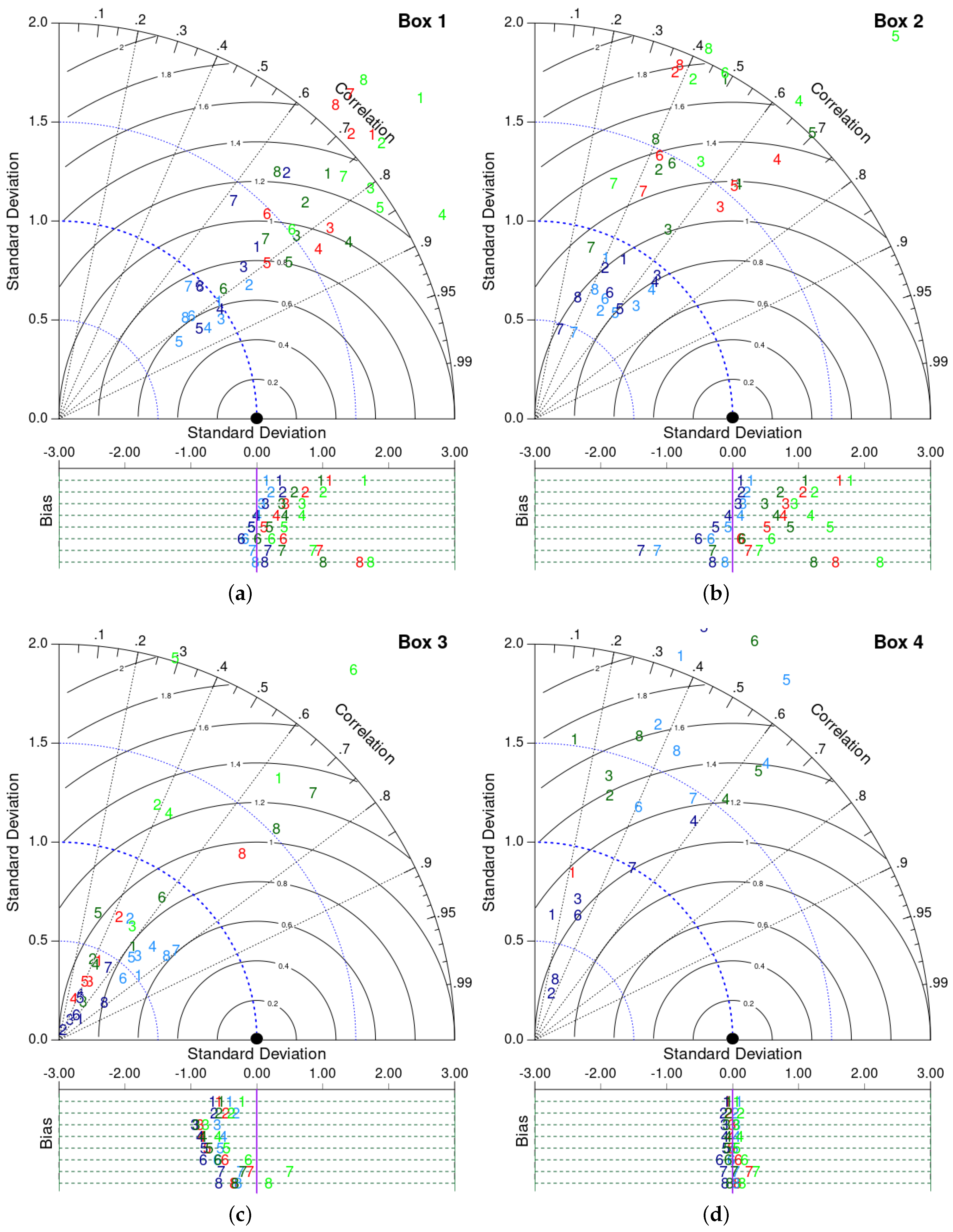
3.3. Statistical Indices
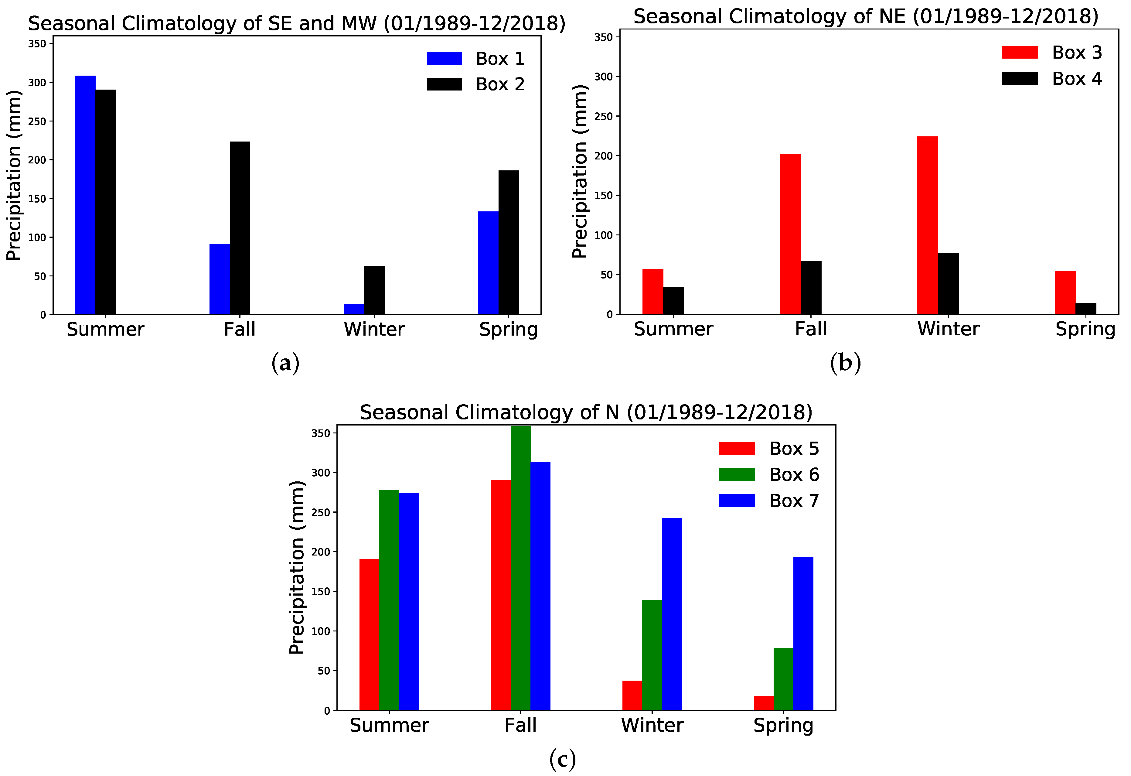
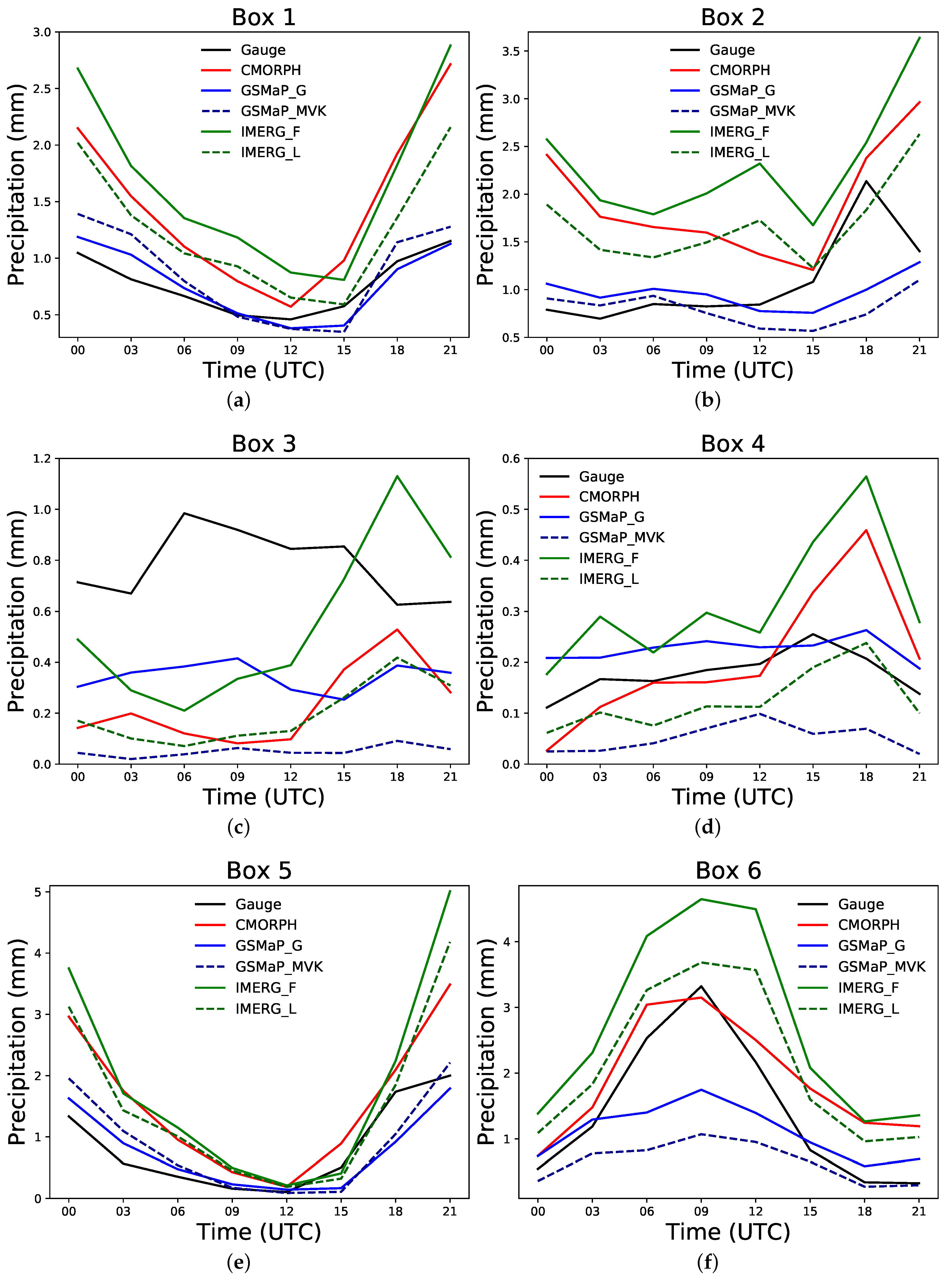
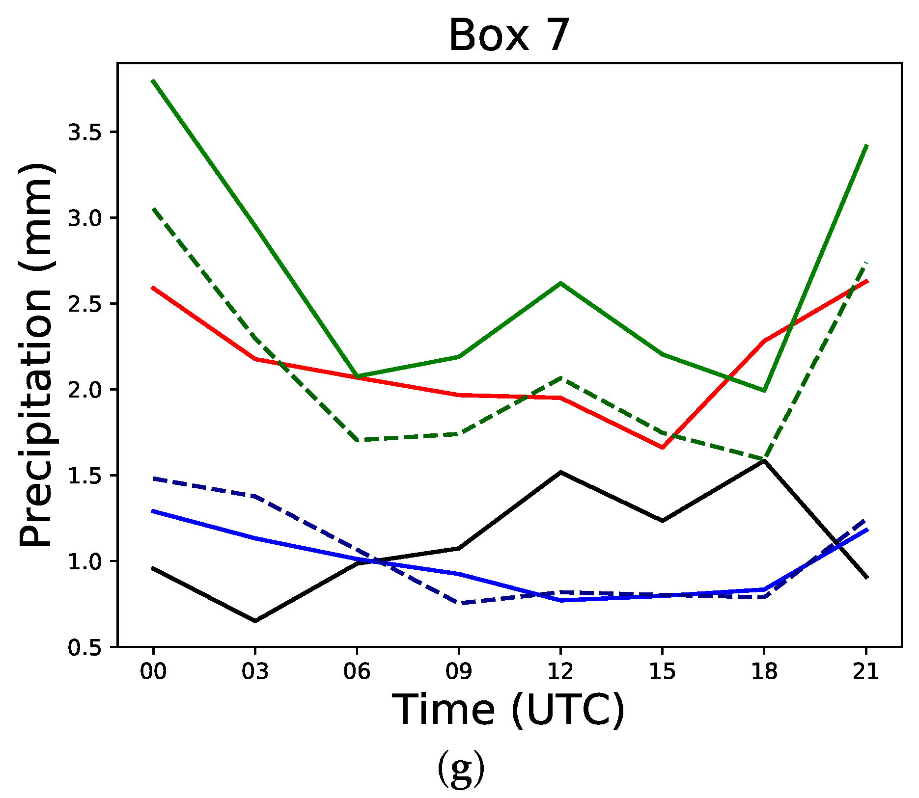
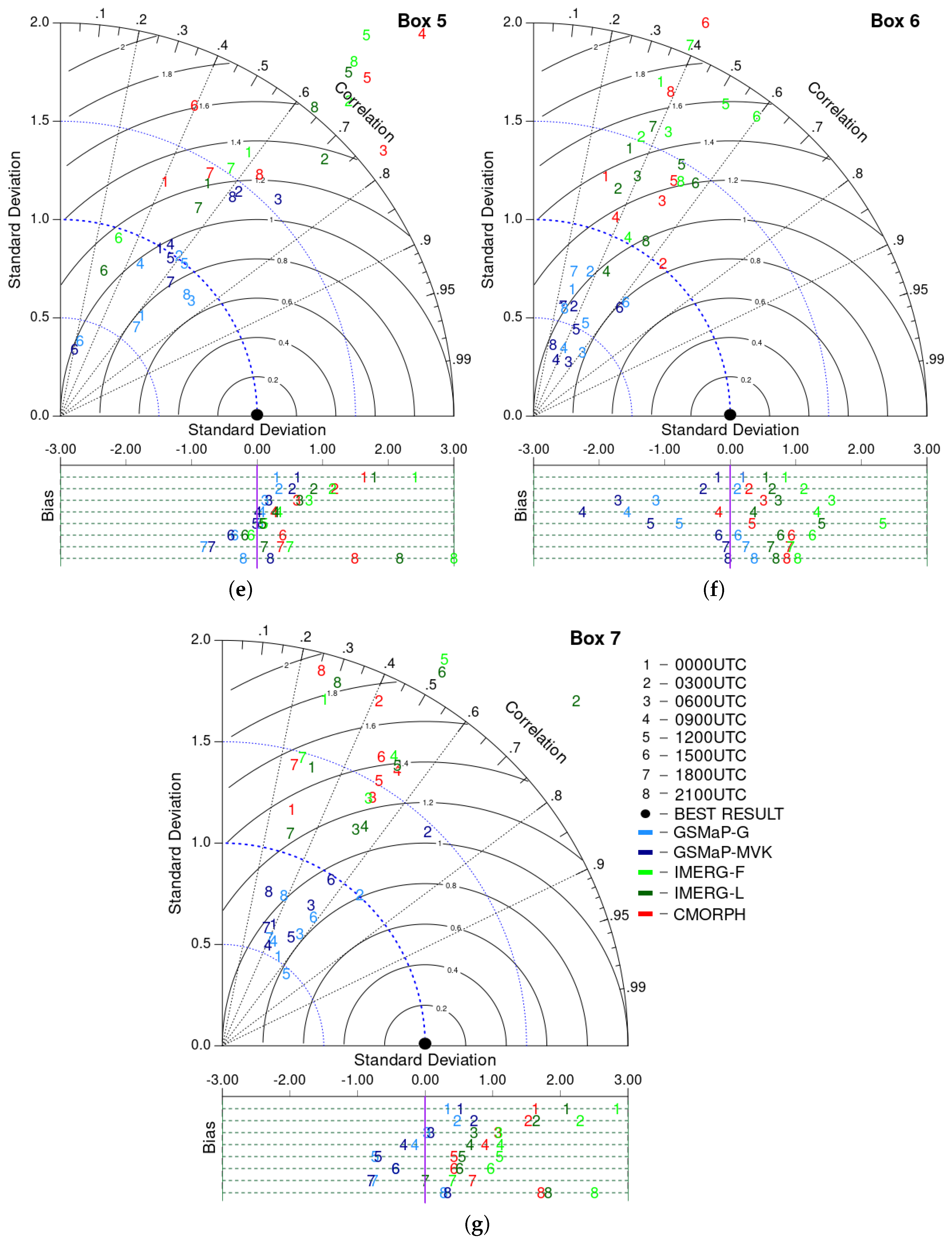
Various statistical indices were used for the regions defined in Section 3.2 in order to compare quantitatively the observations and the estimated precipitation as given by the different algorithms. The equations for the indices as well as their interpretations can be found in Wilks [18] and are summarized in Table 4. Pearson’s correlation coefficient (CC) gives the agreement between the estimated precipitation and the observation at the gauge sites. The root-mean-squared error (RMSE) is used to measure the mean magnitude of the error while the standard deviation (SD) is used to measure the dispersion of the results for a given algorithm. Finally, the bias was used to calculate the systematic and aleatory components of the error in the algorithm products. For each hour, all indices are presented in the tables and highlighted in the Taylor [40] diagrams, after normalization as in Taylor [41].
Notation: n is the sample size; Si is the SPE estimated precipitation; Gi is the gridded reference data (gauges).

4. Results

Precipitation Diurnal Cycle Comparison

Figure 5 show the PDC average values for all algorithms and the reference dataset in the boxes defined in Section 3.2. For a better understanding, the dispersion of mean values (expressed as a normalized value of the standard deviation) for each time is not shown in Figure 5 and it is presented separately in Table 5 and in Figure 6.
The PDC in the first region (box 1), located in the subtropical region and modulated by SACZ and solar heating (maximum during late evening), is quite well represented by all algorithms. All of them could match the time of maximum precipitation (between 2100 and 0000 UTC) but the minimum value around 12 UTC (0900 LT) tends to be shifted around three hours at 1500 UTC with the exception of CMORPH (Figure 5a). However, the bias among the algorithms (see the first column of Table 5 and the Figure 6a, for all algorithms) is quite different. While CMORPH and IMERG suite overestimate the precipitation for all times (positive bias), GSMAP suite presents the lowest values for almost all times with the best performance for GSMaP-G. This result is expected because GSMaP-G is adjusted with daily gauges which help to reduce the bias. It is also important to note that GSMaP suite also has the larger CC and the less dispersion (lower normalized SD) when compared with the rest of the algorithms (Table 5 and Figure 6a).
The second region (box 2), located in the far west of Amazonian region, is largely influenced by the low level circulation with the enhancement/suppression of SACZ activity as mentioned before. In this case, none of the algorithms could fit, in a suitable way, the main characteristics of the PDC. The relative (and absolute) maximum of precipitation observed at 1800 UTC is not well represented by any algorithm (Figure 5b). This suggest that this dynamically driven precipitation process is not correctly represented by any SPEs. However, GSMaP suite has the better agreement with the reference dataset during the period with minimum values (between 0000–1200 UTC) with minimum bias, larger CC and less dispersion. CMORPH and IMERG suite has a better agreement during the peak hour, while the decrease in the precipitation rates at 2100 UTC is missed by all of them (they show the opposite behavior). It is worth mentioning that CMORPH and IMERG suite have larger dispersion values and smaller CC (when compared with GSMaP) for almost all times showing larger degree of uncertainty in those retrievals (Table 5 and Figure 6b).
Boxes 3 and 4 (Figure 5c,d, respectively) are located in the northeastern region of Brazil. The diurnal cycle (PDC) of this region and the physical drivers associated with this regime have been studied by Araujo [42]. In such study, it is clearly stated that the fraction of precipitation from shallow convection is larger than the fraction of precipitation from deep convective and stratiform clouds in a very thin region along the coast which is in a very close match with box 3. The frequency of precipitating deep convection clouds are relatively larger inland but the absolute number of events is much smaller than any other region, resulting in very low values for accumulated precipitation. These results are in good agreement with the results obtained for box 4.
In those regimes, where shallow convection is the main physical driver for precipitation (box 3, in our case), the SPEs tend to fail in retrieving rainfall because ice scattering, the main technique used to retrieve rainfall over the continent, is not efficient for water clouds rainfall retrievals. In that case, almost all algorithms for all times (with the exception of IMERG-F at 1800 and 2100 UTC) underestimate the mean rainfall value (negative bias), Table 5 and Figure 6c. It is also noted that none of the algorithms could represent properly the amplitude and phase of PDC (Figure 5c). It is also well known by the scientific community that water–land transition and shallow convection regimes are among the most difficult challenges that need to be addressed in future versions of the SPEs.
The box 4, mainly located inland over the northeastern region of Brasil, is the region where the lowest average rainfall is observed when compared with other regions (Figure 5d). In this case, most of the algorithms could reproduce those low values of precipitation with low bias (well below 1 mm—see Table 5 and Figure 6d) for all times (note that Figure 5d has a different scale, enhancing the differences among algorithms). However, in general terms, the values of the normalized standard deviation are among the largest values when compared with other regions (Table 5 and Figure 6d). This result suggests a larger dispersion and, consequently, larger uncertainty in the average value (sometimes four times the mean precipitation) which makes it very difficult to evaluate if PDC fits the reference dataset.
The last three boxes, located in the northern region, can be analyzed as the propagation and dissipation of tropical squall lines from the coast to the Amazon region [11,39]. Box 5, located in the continental coast, is mainly driven by a land–sea breeze process and the formation of deep convective clouds after the maximum heating (Figure 5e). The phase of this regime is very well captured by all algorithms (with a peak at 2100 UTC–1800 LT) while the amplitude is better represented by the GSMaP suite (MVK and G) with lower bias and less dispersion (lower standardized SD values), Table 5 and Figure 6e. The transition from a continental coastal to a coastal–inland region (box 6), Figure 5f, mainly driven by the displacement of tropical squall lines inland due to trade winds, is better represented by CMORPH (in phase and amplitude). All other algorithms could also estimate very well the phase of the peak hour at 1200 UTC (0900 LT) but fall short in the amplitude. In this particular case, IMERG suite overestimate the rainfall for all times (with better adjustment for late version), while GSMaP suite underestimate the maximum value and fits better for minimum values (Table 5 and Figure 6f).
The PDC in the last region (box 7) is not well represented by any algorithm (Figure 5g). While the amplitude of GSMaP suite is well represented in magnitude, the phase is the opposite of the observed values. In the case of CMORPH and IMERG suite, all of them overestimate the average precipitation for all times and the phase is completely missed when compared with the reference database (Table 5 and Figure 6g). The dissipation of some of the squall lines formed in the coast and the interaction with the low level circulation is the main factor which modulates the Precipitation Diurnal Cycle.

5. Discussion and Conclusions

This study assessed the ability of several high-resolution satellite-based precipitation estimates to represent the Precipitation Diurnal Cycle (PDC) over Brazil during the 2014–2018 period. In order to perform this task, rigid quality control tests were applied to hourly rain gauge data from different national and regional networks used as the reference dataset, while a hierarchical cluster analysis was applied to rain gauge dataset and yielded seven regions with different PDC characteristics (amplitude and phase) where the performance of three different satellite-based precipitation algorithms (two of them with a gauge-adjusted version) were evaluated during the rainy season of each region.
The performance of all SPEs analyzed are directly related with the characteristics of the most frequent rainy systems acting in a given region. Generally speaking, in those regions where thermal heating produce deep convective clouds (i.e., boxes 1 and 5), the diurnal cycle is better represented in term of amplitude and phase; while the PDC for shallower convection and low-level circulation driven systems (i.e., box 3 and box 7) is poorly characterized by satellite-based retrievals. This result was expected because most of the algorithms relies on ice scattering techniques to retrieve rainfall over land and they fail when the amount of ice is not directly related with the accumulated precipitation. In a recent study of Costa et al. [43] over the Amazonian region showed that the rainfall overestimation error is only function of the Ice Water Path (IWP) and Palharini et al. [44] concluded that shallow clouds are the dominant systems over the Brazilian southeastern coast. Those statements will be discussed in detail for every region.
In those areas where deep convective clouds are responsible for most of the accumulated rainfall in a given region (boxes 1 and 5) and the best results are observed, some differences among algorithms could be pointed out: (i) GSMaP suite performs better than IMERG suite and CMORPH with lower bias, larger correlation coefficient and lower dispersion (blue colors in Table 5; (ii) GSMaP-G is slightly better than GSMaP-MVK due to the inclusion of daily gauges which reduce the bias (mainly during peak hours); (iii) IMERG suite and CMORPH overestimate rainfall for all times (positive bias) and also has a larger dispersion. In the case of IMERG-F (adjusted with monthly rain gauges), it does not outperform the IMERG-L, which suggests that gauge analysis, in this particular case, is not improving the satellite-only retrieval.
The regions located in the Amazonian far from the coast (boxes 2 and 7), where rainfall episodes are characterized by regimes of low-level easterly and westerly winds in the context of the large scale circulation, none of the algorithms could represent, in a suitable way, the amplitude and phase of the diurnal cycle. The IMERG suite and CMORPH (all of them rely on GPROF retrievals for passive microwave sensors) overestimate the observed rainfall. This could be due to the fact, cited by Costa et al. [43] who also used GPROF retrievals in that study, of IWP error estimation which leads in rainfall overestimation. IMERG-L outperform IMERG-F in this region, as also observed in box 1. GSMaP suite has, in general terms, lower bias and lower dispersion (Table 5) when compared with the rest of the algorithms.
The region 3 is dominated by shallow convection clouds which is responsible for most of the accumulated rainfall. With no ice (or very little) in its structure, none of the algorithms could reproduce the diurnal cycle properly with large underestimation of the observed values, mainly during the peak hour (0600 UTC). In this case, gauge-adjusted versions (GSMaP-G and IMERG-F) perform better than the respective satellite-only versions. Region 4, also located in the northeastern Brazil, is where the lowest accumulated rainfall is observed and it has the flattest diurnal cycle in terms of phase and amplitude.
The region 5 is characterized by the transition between a coastal land–sea breeze regime to a continental amazonian regime. In this case, the displacement of tropical squall lines inland generated over the coast, is the main driver for precipitating events. All algorithms, in different degrees of agreement, could represent properly the phase of the diurnal cycle. However, the amplitude is overestimated by IMERG suite (with better results for IMERG-L) and underestimated by GSMaP suite (the bias-adjusted outperform the satellite-only version). CMORPH have the best statistics when compared with other algorithms.
Future research should be centered on understanding how shallow clouds processes and convective/stratiform classification is performed in each algorithm to improve the representation of the diurnal cycle.

Author Contributions

J.M.d.S.A. conceived the structure of this paper writing original draft preparation, D.A.V. and M.A.G. contributed to supervision and to the discussion of scientific problems, D.P.Q., N.d.J.d.C.B., J.H.H.C. and R.S.A.P. contributed to the data processing. All authors have read and agreed to the published version of the manuscript.

Funding

This study was financed in part by and Conselho Nacional de Desenvolvimento Científico e Tecnológico (CNPq) and Coordenação de Aperfeiçoamento de Pessoal de Nível Superior Brazil (CAPES)—Finance Code 001.

Acknowledgments

The authors express their sincere thanks to the scientists responsible for the development of GSMaP, CMORPH and IMERG algorithms. They also acknowledge the National Institute for Space Research (INPE) for the rain gauge data database utilized in this study. The authors are thankful to the Ministry of Telecommunications, Information Technology, and Social Communication of Angola for sponsoring the publication of this article. The second author would like to acknowledge the São Paulo Research Foundation (FAPESP) for supporting this study through the project “Hydrometeorological Monitoring System (HMS) Based on Remote Sensing Products—2018/11160-2”.

Conflicts of Interest

The authors declare no conflict of interest.

Abbreviations

The following abbreviations are used in this manuscript:
PDCPrecipitation Diurnal Cycle
TCThermal Convection
QCQuality Control
SPESatellite-based precipitation estimates
IWPIce Water Path
LBLocal Breezes
LTLocal Time
SLSquall Lines
NENortheast
SESoutheast
NNorth
CSConvective Systems
TRMMTropical Rainfall Measuring Mission
DPRDual-frequency Precipitation Radar
GPMGlobal Precipitation Measurement
ITCZIntertropical Convergence Zone
SACZSouth Atlantic Convergence Zone
CEMIGCompanhia Energética de Minas Gerais
SIMEPARSistema Meteorológico do Paraná
IACAgronomic Institute
ANANational Water Agency
INMETNational Institute of Meteorology
FSFrontal Systems
EWEasterly Waves
CCPearson’s Correlation Coefficient
RMSERoot Mean Square Error
SDStandard Deviation
DPADaily Precipitation Amplitude
GOESGeostationary Operational Environmental Satellite

References

  1. Rozante, J.R.; Vila, D.A.; Chiquetto, J.B.; Fernandes, A.d.; Alvim, D.S. Evaluation of TRMM/GPM blended daily products over Brazil. Remote Sens. 2018, 10, 882. [Google Scholar] [CrossRef] [Green Version]
  2. Marengo, J.; Liebmann, B.; Grimm, A.; Misra, V.; Dias, P.S.; Cavalcanti, I.; Carvalho, L.; Berbery, E.; Ambrizzi, T.; Vera, C. Recent developments on the south american monsoon system. Int. J. Climatol. 2012, 32, 1–21. [Google Scholar] [CrossRef] [Green Version]
  3. Hossain, F.; Lettenmaier, D.P. Flood prediction in the future: Recognizing hydrologic issues in anticipation of the Global Precipitation Measurement mission. Water Resour. 2006, 42, 1–5. [Google Scholar] [CrossRef]
  4. Janowiak, J.E.; Kousky, V.E.; Joyce, R.J. Diurnal cycle of precipitation determined from the CMORPH high spatial and temporal resolution global precipitation analyses. J. Geophys. Res. Atmos. 2005, 110. [Google Scholar] [CrossRef] [Green Version]
  5. Westra, S.; Alexander, L.V.; Zwiers, F.W. Global increasing trends in annual maximum daily precipitation. J. Clim. 2013, 26, 3904–3918. [Google Scholar] [CrossRef] [Green Version]
  6. Roca, R.; Alexander, L.V.; Potter, G.; Bador, M.; Jucá, R.; Contractor, S.; Bosilovich, M.G.; Cloché, S. FROGS: A daily 1× 1 gridded precipitation database of rain gauge, satellite and reanalysis products. Earth Syst. Sci. Data 2019, 11, 1017–1035. [Google Scholar] [CrossRef] [Green Version]
  7. Leong, T.M.; Zheng, D. Assessment of GPM and TRMM precipitation products over Singapore. Remote Sens. 2017, 9, 720. [Google Scholar]
  8. Hsu, K.; Gao, X.; Sorooshian, S.; Gupta, H.V. Precipitation estimation from remotely sensed information using artificial neural networks. J. Appl. Meteorol. 1997, 36, 1176–1190. [Google Scholar] [CrossRef]
  9. Tang, G.; Zeng, Z.; Long, D.; Guo, X.; Yong, B.; Zhang, W.; Hong, Y. Statistical and hydrological comparisons between TRMM and GPM level-3 products over a midlatitude basin: Is day-1 IMERG a good successor for TMPA 3B42V7? J. Hydrometeorol. 2016, 17, 121–137. [Google Scholar] [CrossRef]
  10. Mota, G.V. Characteristics of rainfall and precipitation features defined by the tropical rainfall measuring mission over South America. Univ. Utah 2003, 201, 4590–4605. [Google Scholar]
  11. Brito, S.S.D.B.; Oyama, M.D. Daily cycle of precipitation over the northern coast of Brazil. J. Appl. Meteorol. Climatol. 2014, 53, 2481–2502. [Google Scholar] [CrossRef]
  12. Giles, J.A.; Ruscica, R.C.; Menéndez, C.G. The diurnal cycle of precipitation over South America represented by five gridded datasets. Int. J. Climatol. 2019. [Google Scholar] [CrossRef]
  13. Skofronick-Jackson, G.; Petersen, W.A.; Berg, W.; Kidd, C.; Stocker, E.F.; Kirschbaum, D.B.; Kakar, R.; Braun, S.A.; Huffman, G.J.; Iguchi, T.; et al. The global precipitation measurement (GPM) mission for science and society. Bull. Am. Meteorol. 2017, 98, 1679–1695. [Google Scholar] [CrossRef] [PubMed]
  14. Skofronick-Jackson, G.; Berg, W.; Kidd, C.; Kirschbaum, D.B.; Petersen, W.A.; Huffman, G.J.; Takayabu, Y.N. Global Precipitation Measurement (GPM): Unified Precipitation Estimation from Space. Remote Sens. Clouds Precip. 2018, 175–193. [Google Scholar]
  15. Reboita, M.S.; Gan, M.A.; Rocha, R.P.D.; Ambrizzi, T. Regimes de precipitação na América do Sul: Uma revisão bibliográfica. Rev. Bras. Meteorol. 2010, 25, 185–204. [Google Scholar] [CrossRef]
  16. Tenório, R.S.; Cristina da Silva Moraes, M.; Hyuk Kwon, B. Raindrop distribution in the Eastern Coast of Northeastern Brazil using disdrometer data. RBMET 2010, 10, 415–426. [Google Scholar] [CrossRef] [Green Version]
  17. Ahrens, C. Meteorology today: An introduction to weather, climate, and the environment. In Meteorology Today, 6th ed.; Belmont Publishing House: Belmont, TN, USA, 2009; pp. 116–120. [Google Scholar]
  18. Wilks, D.S. Statistical Methods in the Atmospheric Sciences. In International Geophysics Series, 3rd ed.; Academic Press Publishing House: San Diego, CA, USA, 2011; pp. 133–141. [Google Scholar]
  19. Joyce, R.J.; Janowiak, J.E.; Arkin, P.A.; Xie, P. Cmorph: A method that produces global precipitation estimates from passive microwave and infrared data at high spatial and temporal resolution. J. Hydrometeorol. 2004, 5, 487–503. [Google Scholar] [CrossRef]
  20. Ushio, T.; Okamoto, K.; Kubota, T.; Hashizume, H.; Shige, S.; Noda, S.; Iida, Y.; Aonashi, K.; Inoue, T.; Oki, R.; et al. A combined microwave and infrared radiometer approach for a high resolution global precipitation mapping in the GSMaP project Japan. In Proceedings of the 3rd International Precipitation Working Group Workshop on precipitation measurements, Melbourne, Australia, 23–27 October 2006; pp. 5–11. [Google Scholar]
  21. Kubota, T.; Shige, S.; Hashizume, H.; Aonashi, K.; Takahashi, N.; Seto, S.; Hirose, M.; Takayabu, Y.; Ushio, T.; Nakagawa, K.; et al. Global Precipitation Map Using Satellite-Borne Microwave Radiometers by the GSMaP Project: Production and Validation. IEEE Trans. Geosci. Remote Sens. 2007, 45, 2259–2275. [Google Scholar] [CrossRef]
  22. Kummerow, C.; Hong, Y.; Olson, W.S.; Yang, S.; Adler, R.F.; Mc-Collum, J.; Ferraro, R.; Petty, G.; Shin, D.-B.; Wilheit, T.T.; et al. The Evolution of the Goddard Profiling Algorithm (GPROF) for Rainfall Estimation from Passive Microwave Sensors. J. Appl. Meteorol. 2001, 40, 1801–1820. [Google Scholar] [CrossRef]
  23. Kidd, C.; Matsui, T.; Chern, J.; Mohr, K.; Kummerow, C.; Randel, D. Global precipitation estimates from cross-track passive microwave observations using a physically based retrieval scheme. J. Hydrometeorol. 2016, 17, 383–400. [Google Scholar] [CrossRef] [Green Version]
  24. Huffman, G.J.; Bolvin, D.T.; Braithwaite, D.; Hsu, K.; Joyce, R.; Xie, P.; Yoo, S.-H. NASA global precipitation measurement (GPM) integrated multi-satellite retrievals for GPM (IMERG). Algorithm Theor. 2015, 4, 30. [Google Scholar]
  25. Mega, T.; Ushio, T.; Kubota, T.; Kachi, M.; Aonashi, K.; Shige, S. Gauge Adjusted Global Satellite Mapping of Precipitation (GSMaP_Gauge). In Proceedings of the URSI GASS, Bejing, China, 16–23 August 2014; pp. 1–4. [Google Scholar]
  26. Ward, J.H. Hierarchical grouping to optimize an objective function. J. Am. Stat. Assoc. 1963, 58, 236–244. [Google Scholar] [CrossRef]
  27. Kousky, E.V. Pentad outgoing longwave radiation climatology for the South American sector. Rev. Bras. Meteorol. 1988, 3, 217–231. [Google Scholar]
  28. Kodama, Y.-M. Large-scale common features of subtropical precipitation zones (the Baiu frontal zone, the SPCZ, and the SACZ), Part I: Characteristics of subtropical frontal zones. J. Meteorol. Soc. Jpn. 1992, 70, 813–835. [Google Scholar] [CrossRef] [Green Version]
  29. Lenters, J.D.; Cook, K.H. Simulation and Diagnosis of the Regional Summertime Precipitation Climatology of South America. J. Clim. 1995, 8, 2988–3005. [Google Scholar] [CrossRef] [Green Version]
  30. Marengo, J.A.; Fisch, G.; Morales, C.; Vendrame, I.; Dias, P.C. Diurnal variability of rainfall in Southwest Amazonia during the LBA-TRMM field campaign of the Austral summer of 1999. Acta Amazon. 2004, 34, 593–603. [Google Scholar] [CrossRef]
  31. Espinoza, E.S. Distúrbios nos Ventos de Leste no Atlântico Tropical; INPE: São José dos Campos, Brazil, 1996; pp. 149–152. [Google Scholar]
  32. Kousky, E.V. Diurnal rainfall variation in northeast Brazil. Mon. Weather Rev. 1980, 108, 488–498. [Google Scholar] [CrossRef] [Green Version]
  33. Kousky, E.V. Frontal Influences on Northeast Brazil. Mon. Weather Rev. 1979, 107, 1140–1153. [Google Scholar] [CrossRef] [Green Version]
  34. Molion, L.C.B.; Bernardo, S.O. Uma Revisão da Dinâmica das Chuvas no Nordeste Brasileiro. Rev. Bras. Meteorol. 2002, 17, 1–10. [Google Scholar]
  35. Gan, M.A.; Kousky, V.E.; Roupelewski, C.F. The South America Monsoon Rainfall over West-Central Brazil. J. Clim. 2004, 17, 47–66. [Google Scholar] [CrossRef] [Green Version]
  36. Hastenrath, S.; Greischa, L. The monsoonal current regimes of the tropical Indian Ocean: Observed surface flow fields and their geostrophic and wind-driven components. J. Geophys. Res. Oceans 1991, 96, 12619–12633. [Google Scholar] [CrossRef]
  37. Cavalcanti, I.F.d.A. Um estudo sobre interações entre sistemas de circulação de escala sinótica e circulações locais; INPE: São José dos Campos, Brazil, 1982; pp. 98–101. [Google Scholar]
  38. Silva Dias, P.L.; Bonatti, J.P.; Kousky, V.E. Diurnally forced tropical tropospheric circulation over South America. Mon. Weather Rev. 1987, 115, 1465–1478. [Google Scholar] [CrossRef]
  39. Rickenbach, T.M. Nocturnal cloud systems and the diurnal variation of clouds and rainfall in southwestern Amazonia. Mon. Weather Rev. 2004, 132, 1201–1219. [Google Scholar] [CrossRef] [Green Version]
  40. Taylor, K.E. Summarizing multiple aspects of model performance in a single diagram. J. Geophys. Res. 2001, 106, 7183–7192. [Google Scholar] [CrossRef]
  41. Taylor, K.E. Taylor Diagram Primer. 2005. Available online: www.pcmdi.llnl.gov/about/staff/Taylor/CV/Taylor/diagram/primer.pdf (accessed on 3 August 2019).
  42. Araujo, R. Classificação Climatológica das Nuvens Precipitantes no Nordeste Brasileiro Utilizando Dados do Radar a Bordo do Satélite TRMM. Master’s Thesis, INPE, São José dos Campos, Brazil, 2005; pp. 111–117. [Google Scholar]
  43. Costa, I.C.; Machado, L.A.; Kummerow, C. An examination of microwave rainfall retrieval biases and their characteristics over the Amazon. Atmos. Res. 2018, 213, 323–330. [Google Scholar] [CrossRef]
  44. Palharini, A.R.S.; Vila, D.A. Climatological behavior of precipitating clouds in the northeast region of Brazil. Adv. Meteorol. 2017, 2017, 5916150. [Google Scholar] [CrossRef]
Figure 1. Studied region and spatial distribution of rain gauges.
Remotesensing 12 02339 g001
Figure 2. Quality control flow diagram (a) and spatial distribution and percentage of valid data for each grid point downgraded to 0.3° for visualization purposes (b).
Remotesensing 12 02339 g002
Figure 3. Sub regions (boxes) chosen to assess the estimate products determined by an cluster analysis of the Precipitation Diurnal Cycle (PDC) with gauge data. (a) Boxes 1 and 2 in summer; 3 and 4 in winter and 5, 6 and 7 in fall. Histograms of the different groups of PDCs: (b) summer, (c) fall and (d) winter.
Remotesensing 12 02339 g003
Figure 4. Seasonal Precipitation Climatology in the regions of the boxes in (a) SE and MW, (b) NE and (c) N using data from the Brazilian National Institute of Meteorology (INMET) station network for the 30 year period (from January 1989 to December 2018).
Remotesensing 12 02339 g004
Figure 5. Mean PDC for some satellite-based precipitation algorithms for different regions of Brazil. (a) box 1 and (b) box 2 in summer; (c) box 3 and (d) box 4 in winter and (e) box 5, (f) box 6 and (g) box 7 in fall: Global Satellite Mapping of Precipitation (GSMaP)-Gauge (G) in continuous blue line, GSMaP-Motion Vector Kalman (MVK) in dashed dark blue line, Integrated Multi-satellitE Retrievals for Global Precipitation Measurement (GPM) (IMERG)-Final (F) in continuous green line, IMERG-Late (L) in dashed dark green line and Climate Prediction Center (CPC) MORPHing technique (CMORPH) in red line.
Remotesensing 12 02339 g005aRemotesensing 12 02339 g005b
Figure 6. Taylor diagram for the PDCs estimated by the different algorithms for different regions of Brazil. (a) box 1 and (b) box 2 in summer; (c) box 3 and (d) box 4 in winter and (e) box 5, (f) box 6 and (g) box 7 in fall: GSMaP-G in blue, GSMaP-MVK in dark blue, IMERG-F in green, IMERG-L in dark green and CMORPH in red. Numbers refer to time: 1 at 0000UTC, 2 at 0300UTC, 3 at 0600UTC, 4 at 0900UTC, 5 at 1200UTC, 6 at 1500UTC, 7 at 1800UTC and 8 at 2100UTC.
Remotesensing 12 02339 g006aRemotesensing 12 02339 g006b
Table 1. Information on the rain gauge networks. Acronyms of the states of Minas Gerais (MG), Goiás (GO), São Paulo (SP) and Paraná (PR).
NetworkCoveragePeriodResolutionStation N.
INMETAll Brasil2014–20181 h608
ANAAll Brasil2014–20181 h504
CEMIGMG e GO2014–20181 h21
IACSP2017–201820 min128
SIMEPARPR2015–20183 h21
Total 1282
Table 2. Coverage and space-time resolutions of precipitation satellite products used in this study.
ProductPeriodDomainSpatial
Resolution
Temporal
Resolution
Corrected by
Gauges
Main
Reference
GSMaP-G2014–present50°N–50°S0.1° × 0.1°1 hYes[21]
(CPC daily)
GSMaP-MVK2014–present50°N–50°S0.1° × 0.1°1 hNo[21]
IMERG-F2014–present60°N–60°S0.1° × 0.1°0.5 hYes[24]
(GPCC monthly)
IMERG-L2014–present60°N–60°S0.1° × 0.1°0.5 hNo[24]
CMORPH1998–present60°N–60°S0.08° × 0.07°0.5 hNo[19]
Table 3. Information on the regions of the boxes selected for analyzing the Precipitation Diurnal Cycle (PDC).
BoxRegionDomainSeasonN. of Grid Points
1SE23.70°–20.50°S; 51.00°–47.00°WSummer80
2NW9.50°–4.50°S; 74.00°–70.00°WSummer12
3NE10.50°–8.50°S; 36.50°–34.00°WWinter13
4NE8.50°–6.50°S; 36.50°–34.00°WWinter14
5N5.00°–3.00°S; 44.30°–41.30°WFall10
6N3.50°–1.50°S; 58.00°–54.00°WFall3
7N1.00°S–1.50°N; 67.45°–63.30°WFall8
Table 4. List of the statistical indices used to assess the quality of the satellite-based precipitation estimates.
Statistic IndexFormulaUnitPerfect Value
Correlation coefficient (CC) C C = i = 1 n ( G i G ¯ ) ( S i S ¯ ) i = 1 n ( G i G ¯ ) 2 i = 1 n ( S i S ¯ ) 2 1
Root-mean-squared error (RMSE) R M S E = 1 n i = 1 n ( S i G i ) 2 mm0
Normalized Standard Deviation (SD) S D = 1 n i = 1 n ( S i S ¯ i ) 2 mm1
BiasBias = i = 1 n ( S i G ¯ i ) n mm0
Table 5. Statistical indices of PDC for different regions during 2015-2018 period. The algorithms with the best performances are in blue.
BoxTimeGSMaP-GGSMaP-MVKIMERG-FIMERG-LCMORPH
BiasCCSDBiasCCSDBiasCCSDBiasCCSDBiasCCSD
1000.140.811.000.340.751.331.630.752.450.970.741.841.100.742.14
030.220.821.180.400.681.701.000.762.150.570.751.660.740.722.07
060.070.850.960.130.771.210.690.800.960.380.791.520.440.821.68
090.020.870.88−0.010.830.990.690.882.200.430.851.720.300.841.57
12−0.080.840.72−0.080.840.850.410.831.940.190.831.410.110.801.31
15−0.170.790.85−0.230.720.980.230.781.520.020.781.060.400.711.48
18−0.070.700.940.170.621.410.850.761.890.390.751.380.950.672.21
21−0.030.780.820.130.730.981.730.672.301.010.661.671.560.662.12
2000.270.400.890.120.490.931.780.502.611.100.491.971.620.482.46
030.220.520.640.140.420.851.240.421.900.720.441.411.070.371.89
060.160.670.770.090.650.950.940.541.550.490.571.170.810.661.43
090.130.670.88−0.070.660.921.180.642.090.670.661.570.770.681.79
12−0.070.600.67−0.250.610.701.480.692.660.880.702.020.530.651.55
15−0.320.500.70−0.510.510.740.590.482.000.140.471.470.120.431.47
18−1.140.410.48−1.400.270.470.400.321.250.300.310.910.240.431.27
21−0.120.420.72−0.300.330.652.240.432.071.230.401.541.560.381.93
300−0.410.770.52−0.670.720.15−0.220.641.73−0.540.620.61−0.570.450.45
03−0.310.510.71−0.650.380.06−0.380.391.29−0.570.380.44−0.470.440.70
06−0.600.680.58−0.950.470.12−0.770.540.69−0.910.540.23−0.860.470.33
09−0.500.710.67−0.860.410.26−0.580.441.27−0.810.440.42−0.840.340.22
12−0.550.660.56−0.800.450.24−0.460.292.02−0.710.290.67−0.750.400.32
15−0.600.720.45−0.810.570.16−0.130.622.39−0.590.590.89−0.480.372.31
18−0.240.790.74−0.530.560.440.500.754.62−0.210.721.79−0.100.684.30
21−0.280.790.69−0.580.770.300.180.733.60−0.330.721.53−0.360.701.32
4000.100.352.08−0.090.130.640.070.124.55−0.050.131.53−0.080.220.87
030.040.361.71−0.140.330.250.120.283.83−0.070.291.30−0.050.072.68
060.070.272.45−0.120.290.750.060.274.13−0.090.271.390.000.123.43
090.060.641.83−0.110.591.370.110.554.16−0.070.621.56−0.020.423.50
120.030.572.22−0.100.382.260.060.594.20−0.080.641.77−0.020.323.99
15−0.020.411.29−0.200.330.670.180.434.62−0.070.482.300.080.294.01
180.060.551.46−0.140.491.000.360.606.940.030.563.360.250.616.29
210.050.441.63−0.120.320.320.140.304.58−0.040.331.630.070.214.86
5000.290.630.660.620.510.992.420.581.650.790.531.401.630.411.31
030.330.601.020.530.621.461.140.682.170.870.721.881.190.472.49
060.120.750.890.190.711.560.800.833.160.660.842.720.600.772.13
090.070.470.880.010.541.040.340.613.290.290.643.180.270.692.68
120.040.631.00−0.020.570.980.110.632.480.080.642.280.090.672.32
15−0.340.250.40−0.400.210.35−0.100.310.95−0.180.290.770.390.401.72
18−0.820.650.60−0.690.540.880.500.571.570.110.551.270.360.521.45
21−0.210.720.890.210.621.423.010.642.342.180.642.031.490.641.59
6000.190.290.68−0.180.250.580.840.361.820.540.341.450.200.291.27
030.100.360.79−0.410.350.601.120.361.520.640.351.240.290.651.02
06−1.130.610.41−1.700.540.331.550.431.600.730.401.330.510.511.28
09−1.570.410.38−2.25−0.370.311.320.471.030.360.450.82−0.170.381.10
12−0.770.490.54−1.210.440.492.320.521.861.400.511.490.340.511.40
150.120.630.75−0.170.620.711.250.601.900.770.571.440.940.402.18
180.240.270.77−0.070.260.580.920.392.050.620.381.600.900.063.29
210.370.280.57−0.030.260.381.030.531.410.700.541.060.860.391.79
7000.330.530.520.520.390.652.840.281.782.100.311.441.630.281.22
030.480.671.010.730.691.462.300.743.351.650.722.441.530.411.87
060.030.570.670.080.530.821.090.511.420.720.521.261.080.521.43
09−0.150.440.58−0.320.410.551.120.511.660.670.541.290.890.541.61
12−0.750.670.48−0.700.540.631.100.502.200.550.530.630.430.511.52
15−0.440.580.78−0.430.550.980.970.442.840.510.512.140.430.481.63
18−0.750.400.58−0.800.350.620.410.271.480.010.311.100.700.251.43
210.270.380.800.330.290.792.500.332.411.830.301.881.720.251.92

