3D Point Cloud to BIM: Semi-Automated Framework to Define IFC Alignment Entities from MLS-Acquired LiDAR Data of Highway Roads

Abstract

Building information modeling (BIM) is a process that has shown great potential in the building industry, but it has not reached the same level of maturity for transportation infrastructure. There is a standardization need for information exchange and management processes in the infrastructure that integrates BIM and Geographic Information Systems (GIS). Currently, the Industry Foundation Classes standard has harmonized different infrastructures under the Industry Foundation Classes (IFC) 4.3 release. Furthermore, the usage of remote sensing technologies such as laser scanning for infrastructure monitoring is becoming more common. This paper presents a semi-automated framework that takes as input a raw point cloud from a mobile mapping system, and outputs an IFC-compliant file that models the alignment and the centreline of each road lane in a highway road. The point cloud processing methodology is validated for two of its key steps, namely road marking processing and alignment and road line extraction, and a UML diagram is designed for the definition of the alignment entity from the point cloud data.

1. Introduction

Nowadays, reliable and effective information exchange is crucial to any industry. Misinterpretations or delays directly translate into increased cost and time requirements. In the architecture, engineering, and construction (AEC) domain, this effect is accentuated. This field is a heterogeneous mix of different disciplines that are meant to work together. Such a synergy thrives with the presence of a standard ensuring that the data are accessible and usable by everyone involved. This is what shifted the industry toward the adoption of building information modelling (BIM). It acts as a unique source of information, storing all relevant data about the asset. It is not only a repository, but a workflow based on collaboration among disciplines. The model evolves as the asset does, while each team member contributes to its development [1]. An important factor regarding BIM is that its effects are amplified with the complexity and scale of the project. In the case of infrastructure, assets deal with highly complex and heterogeneous information from different sources. BIM for infrastructure has been growing over the last years, and has shown promising results [2,3,4]. This growth is not limited to its applications, but is also extended to its standardization. The Industry Foundation Classes (IFC) is an open standard for creating BIM models designed by buildingSMART, and it has been shifting toward the infrastructure domain over the past years. Its most recent version, IFC 4.3, was released as candidate standard on April 2020 and has been one of the major updates for the schema. While the previous release only included bridges, this new harmonized version also includes railways, roads, ports, and waterways [5]. The efficiency, safety and performance of these assets are affected by all the stages of its life-cycle, from its design to its demolition. The BIM model is capable of incorporating information throughout its evolution. However, as the project complexity scales with its duration, the difficulty to feed data to update the model also increases. As a result, other technologies are used in conjunction with BIM to overcome this issue. Laser scanning provides a way to obtain both accurate geometric representations instead of idealized forms, and to monitor the current state of the asset.

Point cloud to BIM approaches can be used to obtain an as-built model of the asset [6]. While as-design modelling is quite common and usually straightforward, as-built modelling is challenging because of being based on the real outcome of the construction, instead of the idea behind it. Another application is the enhancement of inspection operations performed in the operational and maintenance stage [7]. These inspections are the main source of data regarding the actualized state of the asset (as-is model), and therefore heavily impact its management.

Mobile laser scanning (MLS) is widely used for many infrastructure-related applications, despite still being an emergent technology. There is a vast literature available from the past decade, showing the interest from researchers, infrastructure operators, and administrations on this surveying technology and its capabilities. Some extensive reviews on the applications of laser scanning on infrastructure can be found in [8,9,10,11]. The review from Ma et al. [10] categorizes these applications according to the assets where the information is extracted from, namely: (1) on-road information extraction (road surface, road markings, driving lanes, road cracks, and manholes), and (2) off-road information extraction (traffic signs, light poles, roadside trees, and power lines). One of the most relevant road assets are traffic signs. Their predefined design in terms of material, shape, and size, makes them a common asset to extract information from. Recent approaches combine 2D imagery and 3D point cloud data extracted from mobile mapping systems in order to detect and classify traffic signs along the road [12,13,14], and to assess their visibility and recognizability [15]. There is also relevant research regarding the influence of vegetation in the infrastructure in terms of clearance and visibility disruption [16,17,18], or works focused on detecting several objects along the infrastructure [19,20].

Of greater interest for this work are two of the aforementioned applications: driving lane generation and road marking extraction. Both of them are complementary applications, as the geometric information from road markings can be employed to extract the driving lanes. As road markings have retroreflective properties, the intensity attribute of 3D point clouds (which is directly related with the energy of the emitted pulse once it is reflected back to the sensor) is commonly used to extract and process them [21,22,23]. Wen et al. [24] propose a complete framework for the extraction, classification, and completion of road markings that is able to extract the road markings using a U-Net (encoder-decoder) segmentation network, and then classify them using a hierarchical approach that uses convolutional neural networks (CNN) to classify small size markings. Finally, occlusions and misdetections can be corrected with a context-based completion based on a conditional generative adversarial network (cGAN). As it can be seen, deep learning frameworks are common on the state-of-the-art for road marking extraction in 3D point clouds. Finally, regarding driving lanes extraction, it is worth mentioning the work from Li et al. [25,26], where 3D roadmaps are generated using the information from previously segmented road markings. Then, lane geometries and lane centrelines can be generated, including transition lines. However, this approach does not have into account the modelling of their outputs according to infrastructure standards.

The objective of this paper is to present a semi-automated framework that takes as input a raw point cloud from a mobile mapping system, and outputs a IFC file that represents the centreline of the road (called alignment or main alignment throughout the paper) and the centreline of each road lane (offset alignment). The contributions of this paper can be listed as follows:

(1)

A point cloud-processing method that extracts the road main alignment and offset alignment of a highway road. In order to do so, a method for detection and classification of solid and dashed road markings is also presented. Note that this road marking processing method does not aim to be a contribution by itself, but it is essential for the whole workflow and will be validated to prove that it has state-of-the-art performance.

(2)

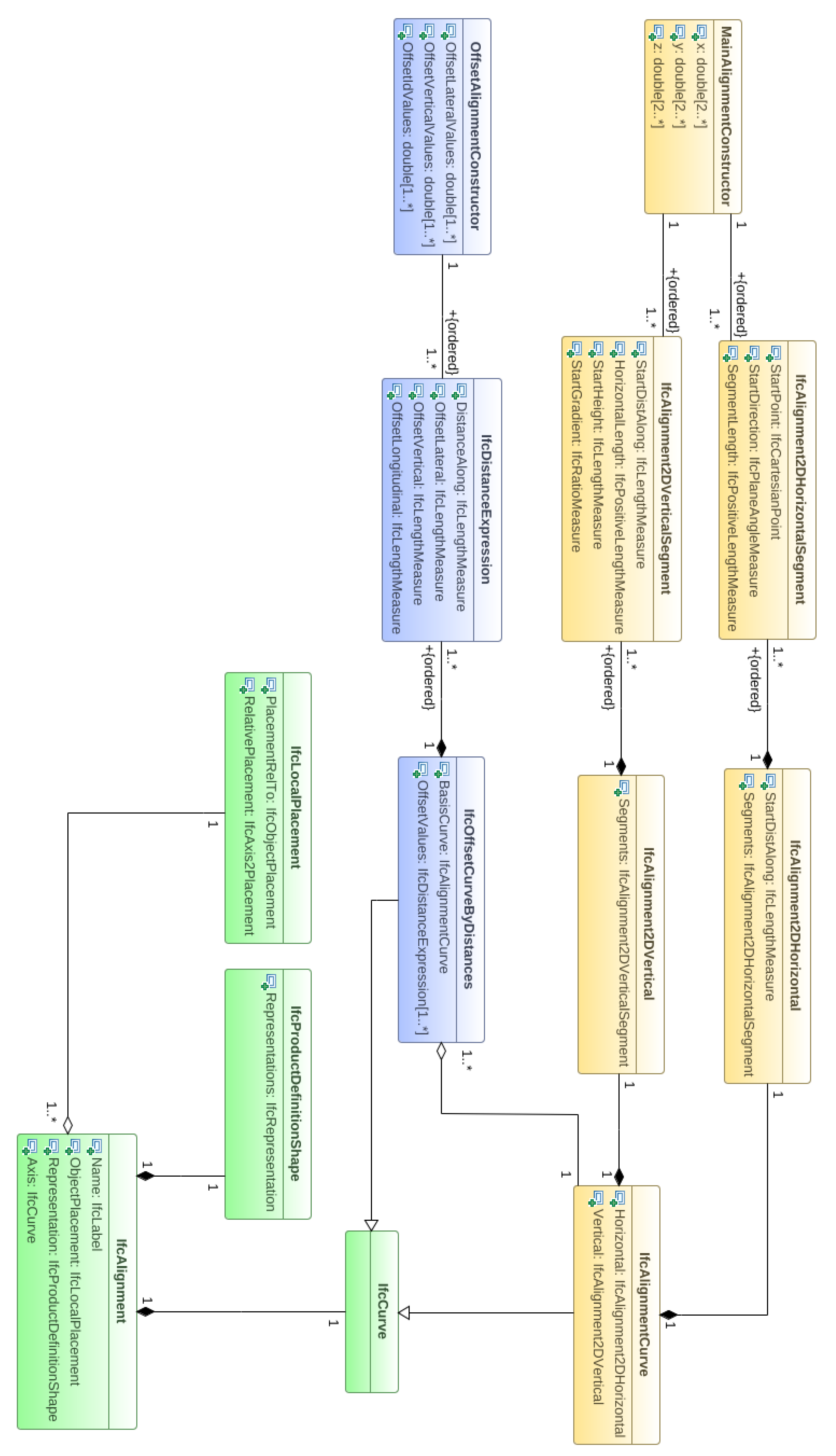
A conversion of the main alignment and offset alignment as exported from the point cloud processing method, to an IFC Alignment model, which is part of IFC 4.1 standard. The model is supported with UML diagrams.

The structure of this paper continues as follows: Section 2 presents the case study data and the proposed methodology, Section 3 shows the results obtained from its validation, Section 4 presents the discussion, and finally Section 5 outlines the conclusions and the future lines of this research.

2. Materials and Methods

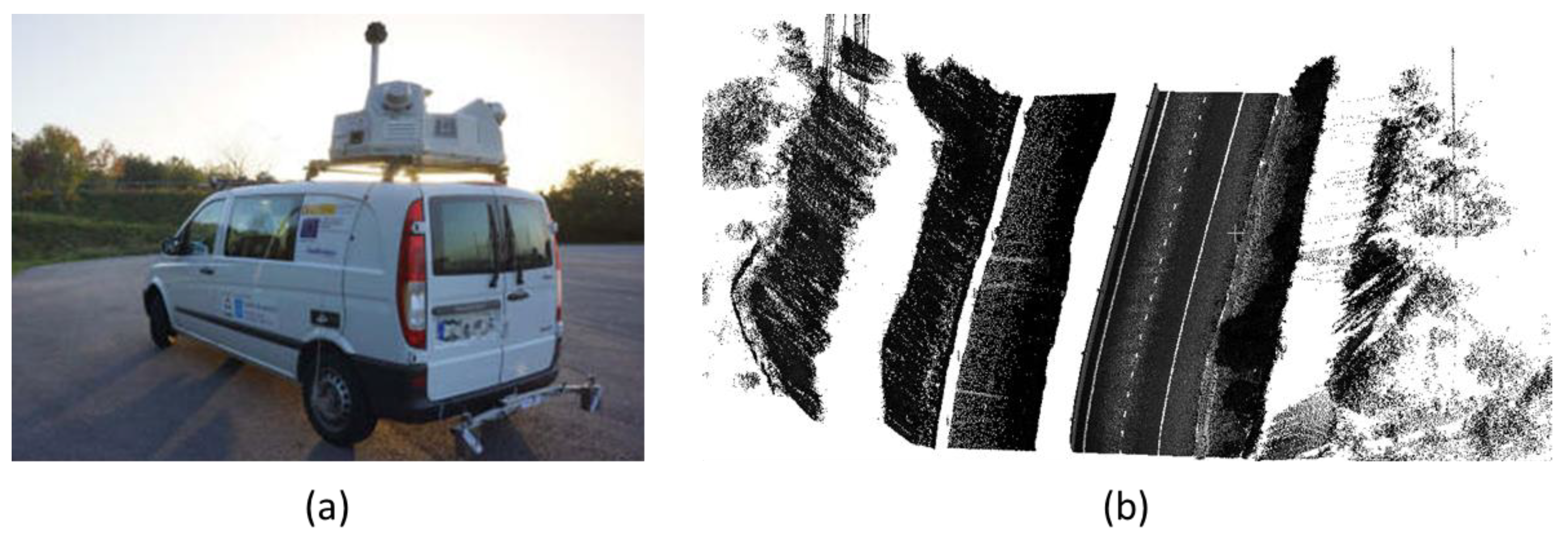
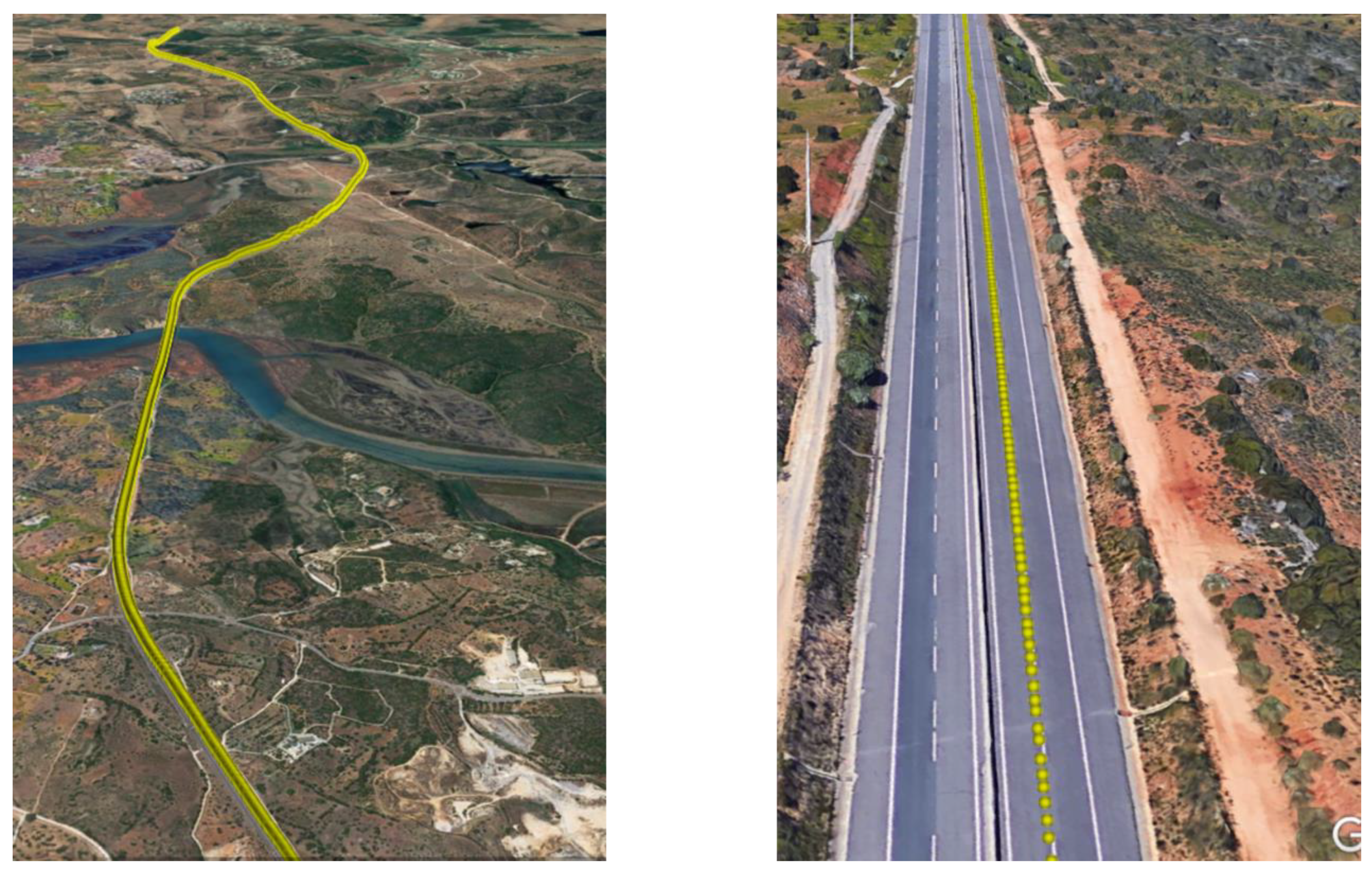
2.1. Case Study Data

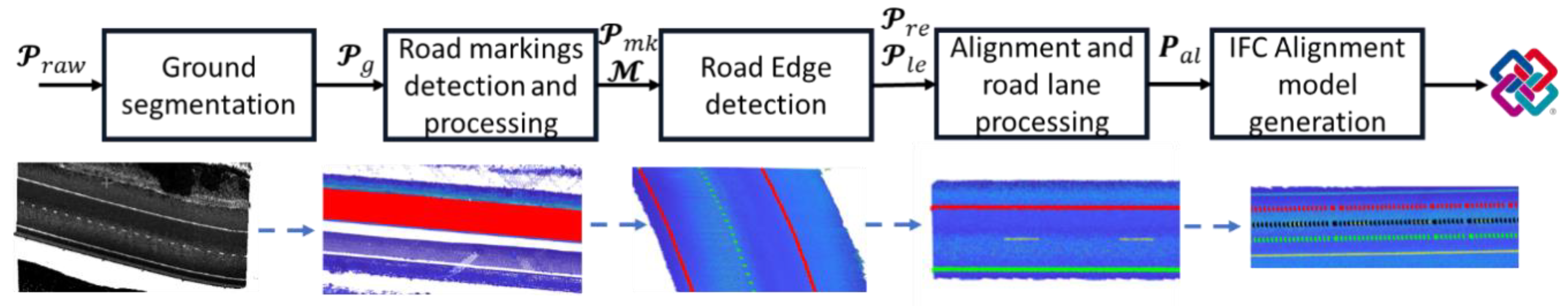
The study area for this work consists of approximately 20 km of a highway road which was surveyed with the LYNX Mobile Mapper by Optech (Figure 1a). It consists of two LiDAR sensor heads, a navigation system that comprises an inertial measurement unit (IMU) and a two-antenna heading measurement system (GAMS), and a LadyBug 5 panoramic camera. For a complete description about the system specifications, the reader is referred to [27].

The raw data of the study area comprise 3D point cloud data as well as trajectory data, both including a synchronized time stamp attribute that allows the georeferentiation of the trajectory with respect to the point clouds. It is important to notice that the size of the point cloud data was too large to be processed with the available equipment, therefore it was divided into 43 individual point cloud sections with a manageable size. In average, each section has 3.5 million points and covers a length of around 400 m (Figure 1b). The complete dataset has approximately 155 million points and covers 17.5 kilometres. The geographic location of the study area is not available because of confidentiality restrictions by the infrastructure owner.

2.2. Methodology

This section presents the methodological approach of this work as a sequential set of processing modules that take as input a 3D point cloud section of a highway road and outputs a IFCAlignment data model according to the specifications of IFC 4.1, which defines the alignment of the road as well as the middle point of each road lane. A schematic diagram of the workflow is shown in Figure 2.

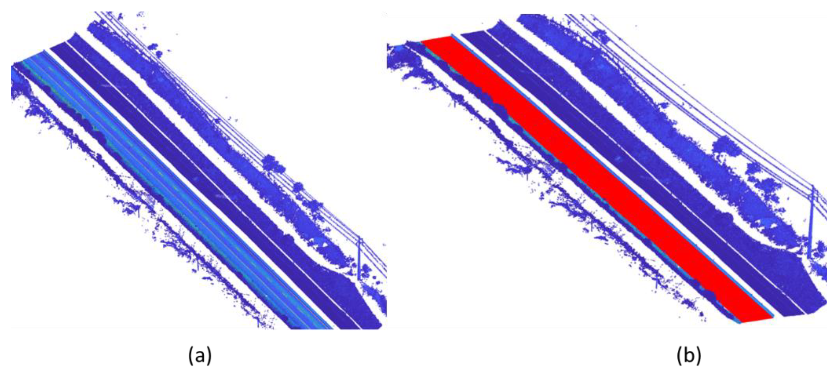
2.2.1. Ground Segmentation

The first module of the methodology aims to isolate the ground in order to ease the subsequent detection of road markings. Let ${\mathit{𝓟}}_{raw}=\left(\mathit{x}, \mathit{y}, \mathit{z}, \mathit{I}, {\mathit{t}}_{\mathit{s}}\right)$ be the raw point cloud, where $\left(\mathit{x}, \mathit{y}, \mathit{z}\right)$ are the 3D coordinates, $\mathit{I}$ is the intensity, and ${\mathit{t}}_{\mathit{s}}$ is the team stamp of the point acquisition. Also, let $\mathcal{T}=\left(\mathit{x}, \mathit{y}, \mathit{z}, {\mathit{t}}_s, \mathit{\varphi }, \mathit{\theta }, \mathsf{\psi }\right)$ be the trajectory of the vehicle during the survey, where $\left(\mathit{x}, \mathit{y}, \mathit{z}, {\mathit{t}}_{\mathit{S}}\right)$ are the 3D coordinates and time stamp in the same coordinate system as the point cloud, and $\left(\mathit{\varphi }, \mathit{\theta }, \mathsf{\psi }\right)$ are the roll, pitch, and heading of the vehicle at each recorded trajectory point. Also, let $\mathcal{S}\left(\mathit{P}, \mathit{i}\right)$ be a function that takes a point cloud $\mathit{P}$ and selects a subset of points with indices $\mathit{i}$ (each index is an integer value representing the position of a point in $\mathit{P}$).

Ground segmentation is a common process in the point cloud processing literature, and there are several different valid approaches to achieve acceptable results for this application. Here, an adaptation of the voxel-based method of Duillard et al. [28] is employed. First, the point cloud ${\mathit{𝓟}}_{raw}$ is voxelized, and each voxel includes the vertical mean and variance of the points within each voxel. Then, a set of ground seed points is selected using the trajectory, and the knowledge that trajectory points are always located directly over the ground. Finally, a region growing algorithm is applied, iteratively selecting the neighboring voxels of those selected as ground and adding them to the ground segment when their vertical mean and variance are under thresholds $d_{\mu }$ and $d_{\sigma } .$

Once the region growing is finished, the indices of the points within the voxels selected as ground, ${\mathit{i}}_g$, are retrieved, and the ground cloud is defined as ${\mathit{𝓟}}_g\mathcal{S}({\mathit{𝓟}}_{raw},{\mathit{i}}_g)$. In practice, only the indices are stored in memory, such that ${\mathit{𝓟}}_g$ is generated from ${\mathit{𝓟}}_{raw}$ only when it is needed. A more detailed description of the whole ground segmentation process can be found in previous work [12]. Figure 3 shows the results of the ground segmentation process.

2.2.2. Road Markings Detection

The objective of this module is to detect points that belong to road markings within the previously segmented point cloud ${\mathit{𝓟}}_g$. Here, a detection process based on point intensity is proposed, as it is a highly discriminative feature that allows separating pavement and road markings. The following considerations are made to design the process of this module:

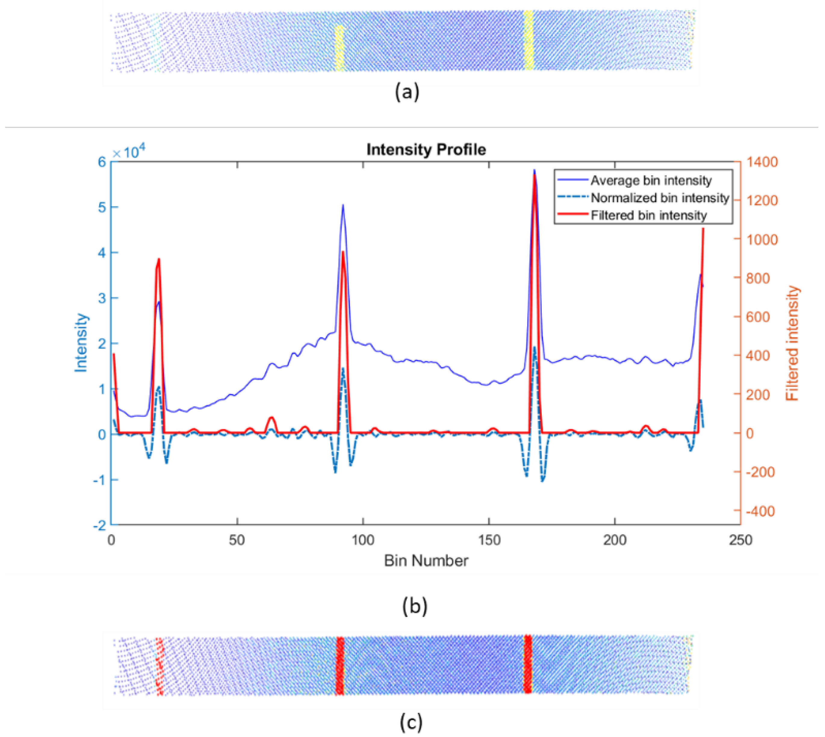
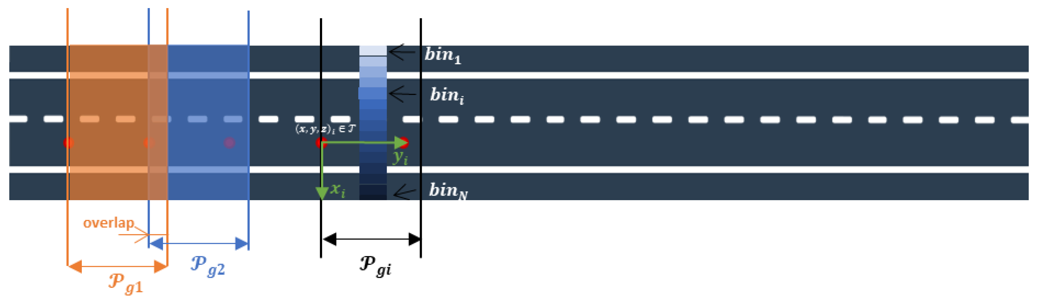
• The intensity of a point is an attribute that depends on the distance between the sensor and the point itself. Therefore, usage of global intensity thresholds is not feasible. Instead, the intensity attribute should be analyzed locally, among points with similar distance with respect to the sensor.
• Most of the markings are linear elements that follow the direction of the vehicle trajectory (solid and dashed lines). Therefore, it seems convenient to locally search for road markings in a set of slices parallel to the trajectory.
• The generation of those slices needs to have into account the curvature of the road. The longer the slice in the direction of the trajectory at a point, the larger the effect of the curvature of the road. Hence, it is preferable to define short slices and process them iteratively.

With these considerations, the point cloud ${\mathit{𝓟}}_g$ is divided into a number of sections following the trajectory of the vehicle. For each point ${\left(x, y, z\right)}_i\in \mathcal{T}$, a geometric transformation is applied to both the point cloud and the trajectory. First, they are translated such that the origin of coordinates corresponds to ${\left(x, y, z\right)}_i$ and then rotated around the Z axis an angle given by the trajectory heading, ${\psi }_i$, such that the next point ${\left(x, y, z\right)}_{i+1}\in \mathcal{T}$ is located along the Y-axis. Then, the indices ${\mathit{i}}_{gi}$ of the points with Y coordinates in the range $[0, y_{max}]$ are obtained and the point cloud ${\mathit{𝓟}}_{gi}=(P_{\mathit{g}i},{\mathit{i}}_{gi})$ is extracted, where $y_{max}$ is the y coordinate of ${\left(x, y, z\right)}_{i+1}\in \mathcal{T}$ plus an overlap of 2 m set to avoid losing points in curved areas of the road. Then, each ${\mathit{𝓟}}_{gi}$ is subsequently divided, following the same process, in bins $[bi{n}_1, bi{n}_2\dots bi{n}_i, \dots bi{n}_N]$ of length $bi{n}_l$ (with $bi{n}_l/2$ of overlap), and width $bi{n}_w$. This process is graphically illustrated in Figure 4.

The average intensity value of the points within each bin will be used to generate intensity profiles of the road. As it was mentioned, the intensity of a point depends on the distance with respect to the sensor, so the intensity profile is normalized by subtracting the average ground intensity across the profile. Then, in order to find consistent intensity peaks, the intensity profile is smoothed with a gaussian-weighted moving average filter with window size $w_g$, and with a top-hat filter with a filter size $w_{th}$. Finally, peaks are selected as local maxima with values higher than the intensity average across all bins. First and last bins are removed from the peak selection to avoid boundary artifacts. Points within bins selected as peaks are considered road marking candidates (Figure 5).

Once every ${\mathit{P}}_{gi}$ has been analyzed, the road marking candidates are clustered via Euclidean distance clustering. As every bin selected during the process may have both road marking and pavement points, the latter are removed by applying an Otsu thresholding [29] to each cluster and its neighboring points, in a neighborhood $n_s$. This process results in a set of indices ${\mathit{i}}_m$ that allow the selection of a point cloud ${\mathit{𝓟}}_{mk}=\mathcal{S}({\mathit{𝓟}}_{raw},{\mathit{i}}_{mk})$ with the detected road markings (Figure 6).

2.2.3. Road Markings Processing

The objective of this module is to assign semantics to the points detected as road markings in the previous step of the methodology. The following considerations have been made:

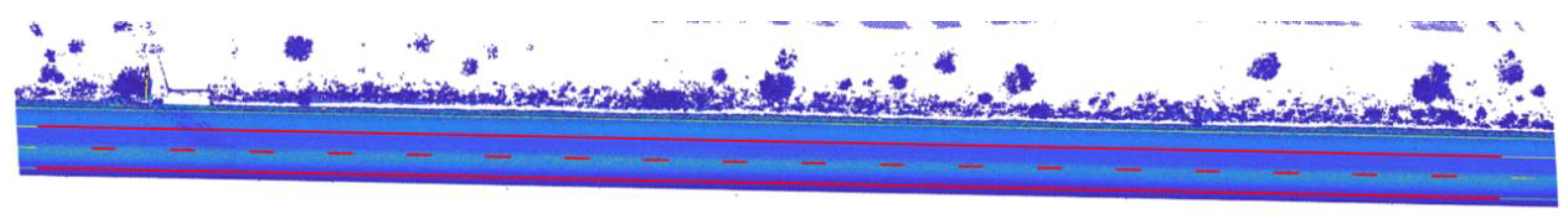
• The main objective of the whole process is to extract the center of the road and each lane using the information given by the road markings. Therefore, the relevant markings to be classified are solid and dashed lines.
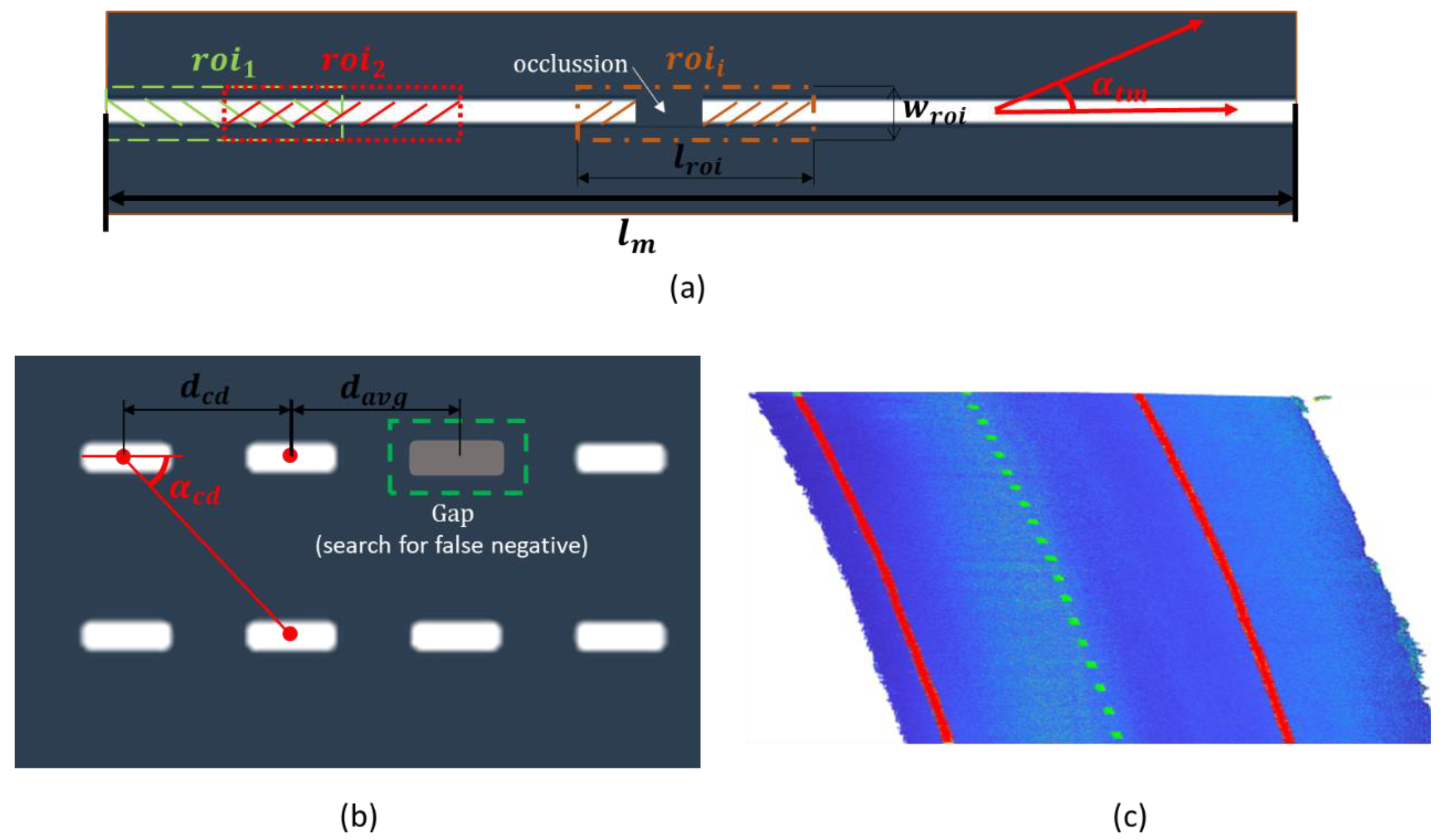
• The knowledge about the semantics of the road markings will allow to analyze the presence of false positives as well as occlusions and other false negatives on the point cloud of detected road markings, ${\mathit{𝓟}}_{mk}$.

First, the point cloud ${\mathit{𝓟}}_{mk}$ is retrieved from the indices extracted in the previous step. Then, it is rasterized, following the rasterization approach in [30] with a raster size $r_s$; and a binary image representing the pixels that contain at least one point is generated. Then, the eccentricity of each connected component is computed. The eccentricity is defined as the ratio of the distance between the foci of the ellipse that has the same second-moments as the connected component, and its major axis. Only those components with an eccentricity close to 1 (larger than $ec{c}_{th}$), hence elongated elements, are selected as either solid or dashed lanes. A soft length filter is applied, initially classifying as dashed those lines whose length is between $das{h}_{th}$ and $soli{d}_{th1}$, and solid if they are longer than $con{t}_{th}$. This soft thresholding allows to apply different processing approaches to solid and dashed lines to achieve a final classification result.

For each solid line in ${\mathit{𝓟}}_{mk}$, a Gaussian Mixture Model (GMM) fits the intensities of the points of ${\mathit{𝓟}}_{mk}$ and its neighborhood in ${\mathit{P}}_g$ to two different classes (ground and road marking). Then, a region growing process is defined to detect false negatives or partially occluded areas of the lines, where rectangular regions of interest $\left[ro{i}_1,ro{i}_2,\dots ro{i}_i,\dots ,ro{i}_N\right]$ centered on the line are iteratively defined, following the direction of the line until no more points are found. Each $ro{i}_i$ is defined to have a length of $l_{roi}$ and a width, $w_{roi}$, equal to two times the width of the line. The intensity of the points within each region is classified using the GMM, and every point classified as road marking that is not found in the original solid line is added to it. This step allows to merge solid lines separated by an occluded area and to refine the detection of road marking points in the direction of the line. This process is illustrated in Figure 7a.

Finally, to deal with false positives, each solid marking is set to meet two conditions: First, since the solid line has to be parallel to the trajectory, the angle ${\alpha }_{tm}$ between their principal directions is computed and markings whose angle is larger than ${\alpha }_s$ are considered false positives. Similarly, markings whose length $l_m$ is shorter than $soli{d}_{th2}$ are considered false positives as well (Figure 7a). Note that $soli{d}_{th1}<soli{d}_{th2}$, as the previous step is expected to reconstruct solid markings with small occlusions.

Regarding dashed markings in ${\mathit{𝓟}}_{mk}$, the objective is to find all markings that belong to the same line, considering that there may be more than one road lane separated with dashed markings. First, length and width of all dashed markings is computed, and they are clustered in groups such that the length and width of each marking is closer than tolerances $t_l$ and $t_w$ to the average value for all markings in the cluster. For the markings within each cluster, they are iteratively analyzed computing (1) the angle ${\alpha }_{cd}$ between the principal direction of the dashed marking and the direction of the vector that joins its centroid with the centroid of the closest marking in the cluster, and (2) the distance $d_{cd}$ between centroids (Figure 7b). Two markings are merged as part of the same line when these parameters are under thresholds ${\alpha }_{th}$ and $d_{th}$.

Finally, a process to search false negatives is carried out. The average of the minimum distances between the centroids of two markings within the same line, $d_{avg}$ is computed, and when a gap is found between the two consecutive markings, the position of the missing ones is obtained using the aforementioned distance and the direction of the line (Figure 7b). In order to detect only the points belonging to the dashed marking, a rectangular region is computed and a binary intensity classification of the points within the region in ${\mathit{P}}_g$ (using a GMM in an analogous manner than for solid lines) is applied.

Once solid and dashed lines are processed, they are stored as objects with several properties as shown in

Table 1. Properties of each road marking object in $\mathit{ℳ}$.

Property	Description
path	Path of the point cloud ${\mathit{𝓟}}_{\mathit{r}\mathit{a}\mathit{w}}$
indices	Indices of the marking in ${\mathit{𝓟}}_{\mathit{r}\mathit{a}\mathit{w}}$
points	Nx3 array with the coordinates of the marking
class	Class of the marking (solid, dashed, or others)
geometry	Geometric properties of the marking
line	Polynomic parametrization of the marking

. That is, for each ${\mathit{𝓟}}_{mk}$, a set of road markings $\mathit{ℳ}=[M_1,\dots ,M_i,\dots ,M_n]\in {\mathit{𝓟}}_{mk}$ are defined with semantics and relevant properties. Note that not all properties are computed at this stage, and also that road marking points that are not classified as neither solid or dashed are considered of class “Others” but still stored as part of the output of this module. Road markings $M_i$ of a road section are shown in Figure 7c.

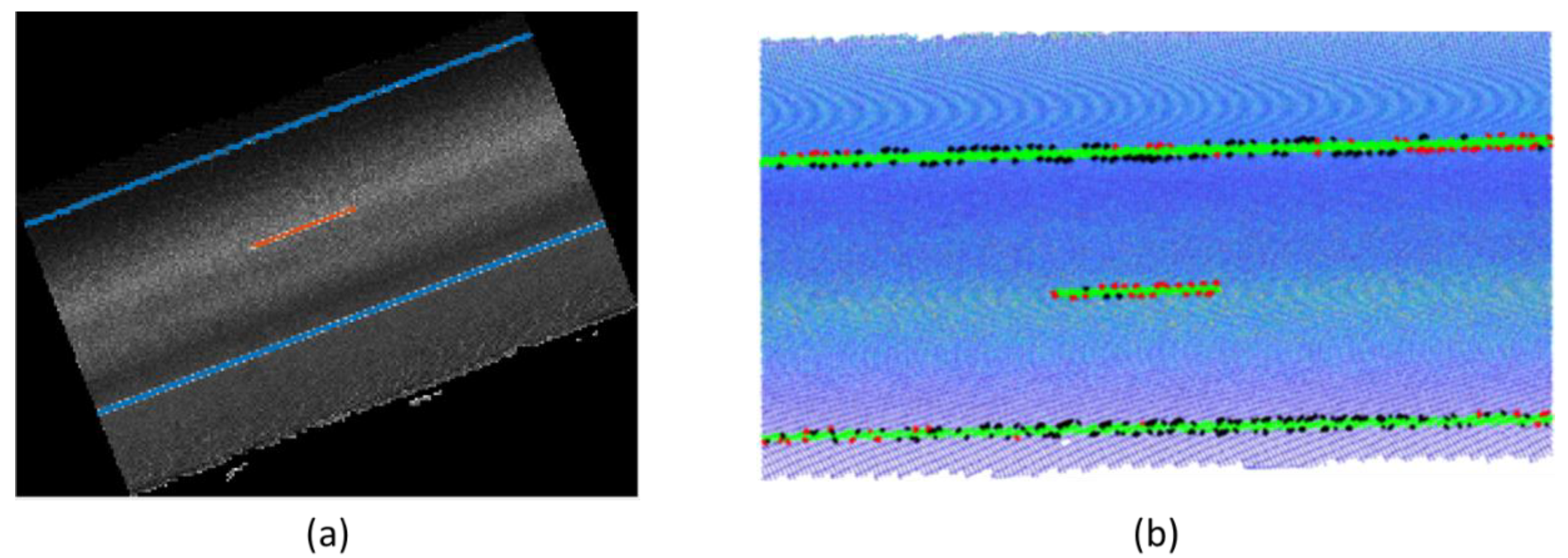
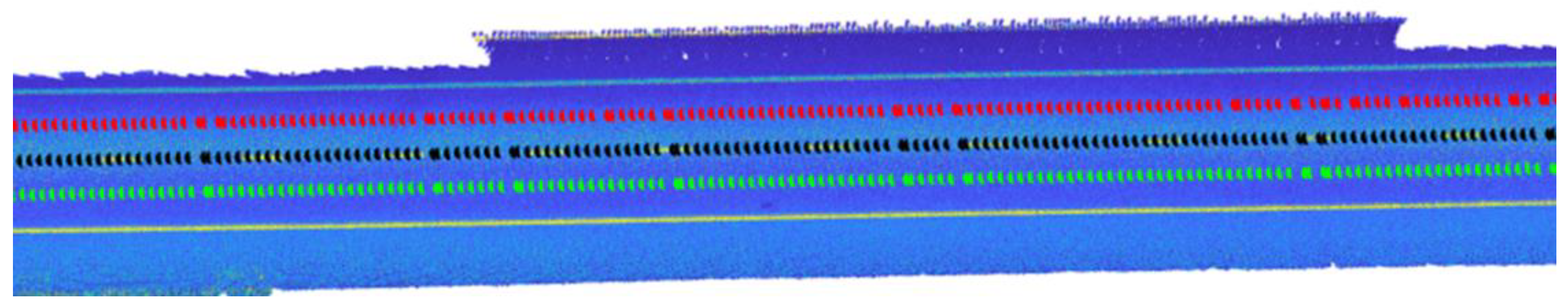
2.2.4. Road Edge Detection

This module aims to detect those road markings that delineate the edges of the road. The precise knowledge of road edges is essential to extract the center point of the road and hence, to build the IFC alignment models. The following considerations have been made:

• The geometric data that are exported to build the IFC alignment model must not contain any error, so the model can be created correctly. This will be ensured if road edges are detected with no errors.
• A fully automated approach is not desirable for this module. Even if complex heuristics are defined, it is not possible to ensure that road edges are correctly detected in all cases. Therefore, an efficient approach would include an automated process with manual verification, and only in those cases when errors are detected, a manual delineation of road edges would be enabled.
• Manual verification of the results allows the definition of simple heuristics that are able to efficiently detect road edges in most cases, even if they are not robust enough to perform correctly in all cases.

With these considerations, an automatic road edge detection process is defined, and the results for each point cloud ${\mathit{𝓟}}_{raw}$ are manually verified by the user. If errors are found, the user is asked to manually select the road edges.

Regarding the automatic process, markings $\mathit{ℳ}$ as computed in the previous module are retrieved together with the ground point cloud ${𝓟}_g$ and the trajectory $\mathcal{T}$. Then, ${\mathit{𝓟}}_g$ is divided following the direction of the trajectory, retrieving the sections ${\mathit{𝓟}}_{gi}$ as detailed in Section 2.2.2. Then, the spatial coordinates of each road marking within ${\mathit{𝓟}}_{gi}$ are defined, obtaining a subset ${\mathit{ℳ}}_i=\left[M_1, \dots M_j, \dots M_N\right]\subset \mathit{ℳ}$. Each $M_j$ is analyzed, computing its length $L_{Mj}$ and its transversal distance with respect to the trajectory $D_{Mj}$. Note that this distance is defined as negative if it is measured to the left in the direction of the trajectory, and positive otherwise). Those $M_j$ whose $L_{Mj}$ is smaller than the 90% of the section length are filtered out, and from the remaining $M_j$ those with largest positive and negative $D_{Mj}$ are selected as part of the right edge and left edge respectively.

These heuristics are simple but efficient. The result should be correct unless there exist false positives outside of the road edges or the edges themselves are false negatives. For these cases, the user will be asked to delineate road edges, selecting a rectangular region in ${\mathit{𝓟}}_{gi}$ for each edge.

This results, independently of the type of process, in a couple of arrays of indices, (${\mathit{i}}_{re}, {\mathit{i}}_{le})$ allowing the selection of both road edges such that ${\mathit{𝓟}}_{re}=\mathcal{S}({\mathit{𝓟}}_g,{\mathit{i}}_{le})$, ${\mathit{𝓟}}_{le}=\mathcal{S}({\mathit{𝓟}}_g,{\mathit{i}}_{le})$ are the point clouds of the right and left edge respectively (Figure 8).

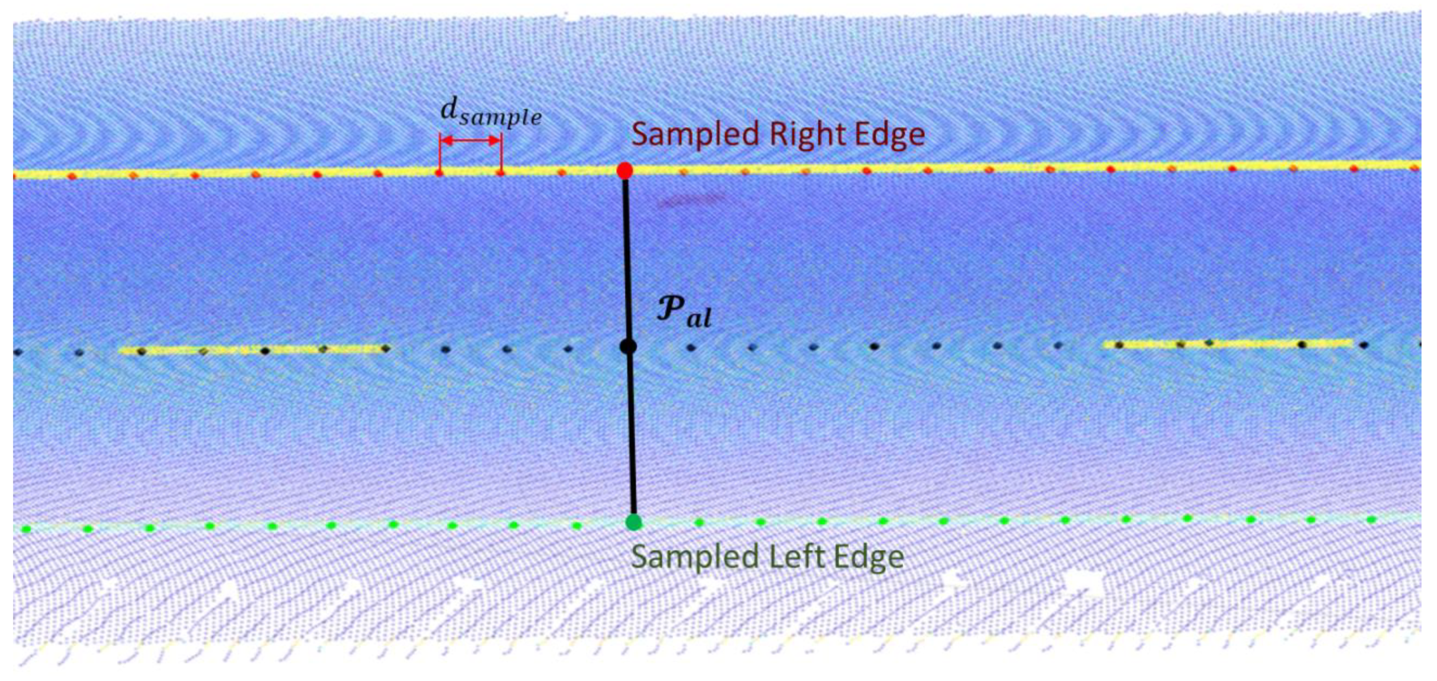
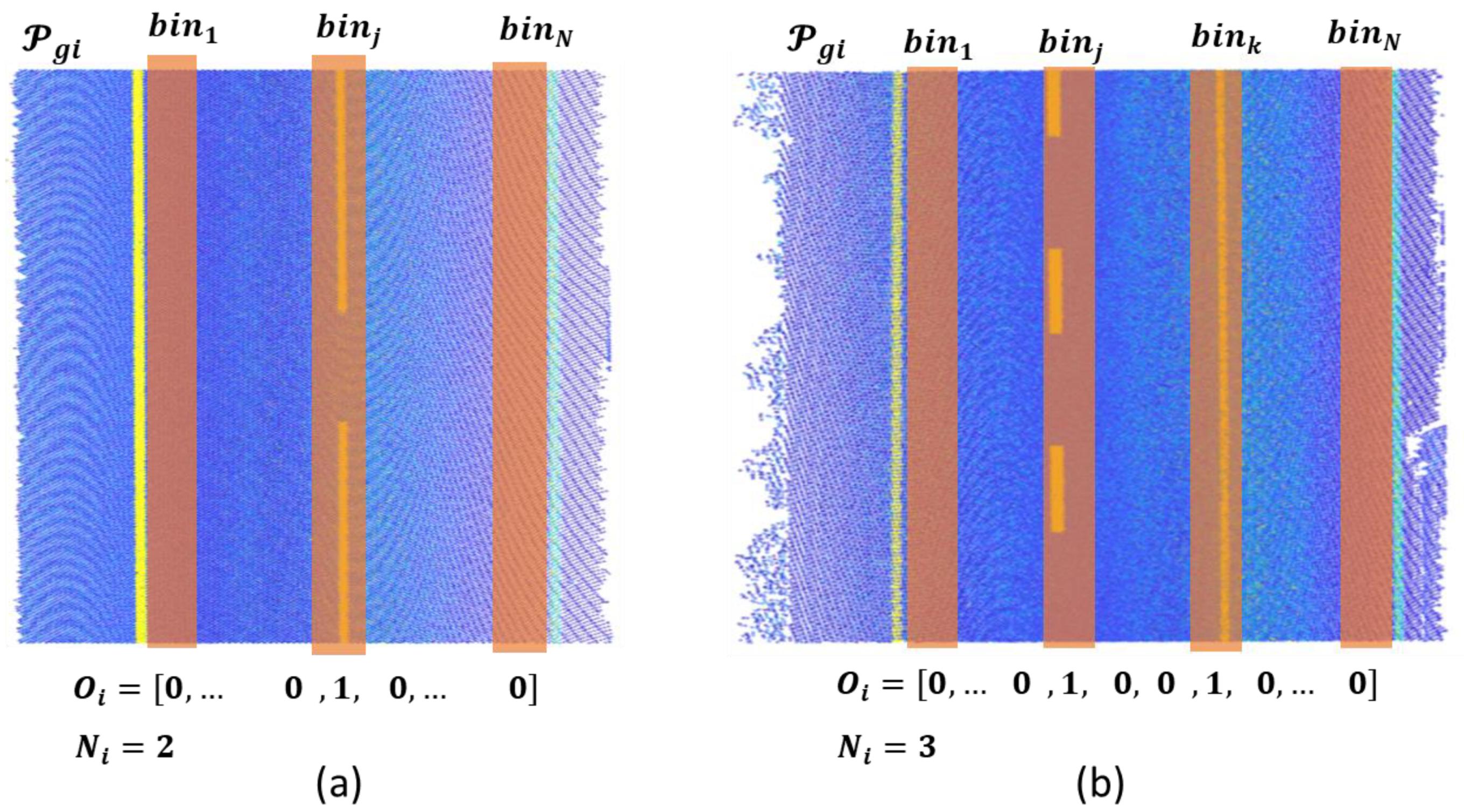
2.2.5. Alignment and Road Lane Processing

The objective of this module is to detect and define the alignment of the road and the centerline of each road line. For that purpose, the point clouds of the road edges ${\mathit{𝓟}}_{re}$ and ${\mathit{𝓟}}_{le}$ are used together with the point cloud of the ground ${\mathit{𝓟}}_g$ and road markings $\mathit{ℳ}$. First, a linear polynomic curve is fitted to the $\left(x,y\right)$ coordinates of each edge. If the quality of fit is good ($R^2$ coefficient larger than $R{2}_{min}$) the linear model is kept. Otherwise, it is replaced by a quadratic polynomic curve, that will get a better fit in curved sections of the road.

The polynomic curves are subsequently sampled, obtaining a point each $d_{sample}$ meters. This results in two sets of coordinates that represent the road edges with a set of uniformly distributed 2D points. In order to retrieve the third coordinate, the closest neighbor in the $\left(x,y\right)$ coordinates of ${\mathit{𝓟}}_g$ is obtained, and the z coordinate of the closest neighbor assigned to the sampled edge point.

Finally, the alignment is defined using the left edge as reference. For each point on the edge, the closest point of the right edge is selected, and the closest point to the geometric mean of both edge points in ${\mathit{𝓟}}_g$ is computed and considered an alignment point (Figure 9). This way, a set of points ${\mathit{P}}_{al}=\left(x,y,z\right)\subset {\mathit{𝓟}}_g$ is defined and will be used to build the IFC alignment model. Note that ${\mathit{P}}_{al}$ coordinates should be ordered following the direction of the trajectory.

Once the coordinates ${\mathit{P}}_{al}$ are retrieved, the middle point of each road lane is computed. First, it is necessary to make some considerations:

• The first necessary step is to detect the number of road lanes. This number is not constant along the study area, and a single point cloud ${𝓟}_g$ may have different numbers of lanes when, for instance, there is a highway entrance or exit.
• Both solid and dashed markings can separate two lanes. However, the separation between the same lines can change along the road (for instance, a dashed line can be replaced by a solid line for a road section with prohibition of overtaking).

With these considerations, the point cloud ${\mathit{𝓟}}_g$ is transversally divided in sections ${\mathit{𝓟}}_{gi}$ and subsequently in bins $\left[bi{n}_1, bi{n}_2\dots bi{n}_j, \dots bi{n}_N\right]$ following the same approach than in Section 2.2.2, but defining each bin with the same length than ${\mathit{𝓟}}_{gi}$ and a width of $bi{n}_{w2}$, and considering only bins between the edges ${\mathit{𝓟}}_{re}$ and ${\mathit{𝓟}}_{le}$. Then, an occupancy vector ${\mathit{O}}_i=[O_1, O_2, \dots , O_j,\dots ,O_n]$ is computed such that ${\mathit{O}}_i$ indicates whether or not there are either solid or dashed markings from $\mathit{ℳ}$ in $bi{n}_i$. The presence of markings in a bin indicates a separation between two lanes, hence $O_i$ indicates how many road lanes are in ${\mathit{𝓟}}_{gi}$ (Figure 10). The number of lanes ${\mathcal{N}}_i$ in each ${\mathit{𝓟}}_{gi}$ is stored in an array $\mathcal{N}=[N_1, \dots , N_i, \dots N_N$], and it is analyzed with the following criteria: (1) the number of lanes has to be constant for a distance of at least $d_{lane}$. If any discrepancy is found in the number of lanes $N_i$ of a section ${\mathit{𝓟}}_{gi}$, it is assumed to has the same number of lanes as the previous correct section.

Finally, the middle point of each road lane is obtained following the same approach than for the alignment coordinates ${\mathit{P}}_{al}$, starting on the left margin and computing iteratively the middle point with respect the next lane separation until the right margin is reached.

At this point, two different tables are created as .csv files to export the results. The first one includes a Nx3 matrix with the coordinates of ${\mathit{P}}_{al}$ as a set of ordered 3D points defining the center of the road with a small resolution. The second one is a Mx3 matrix that allows the positioning of the middle point of each road lane from ${\mathit{P}}_{al}$, including:

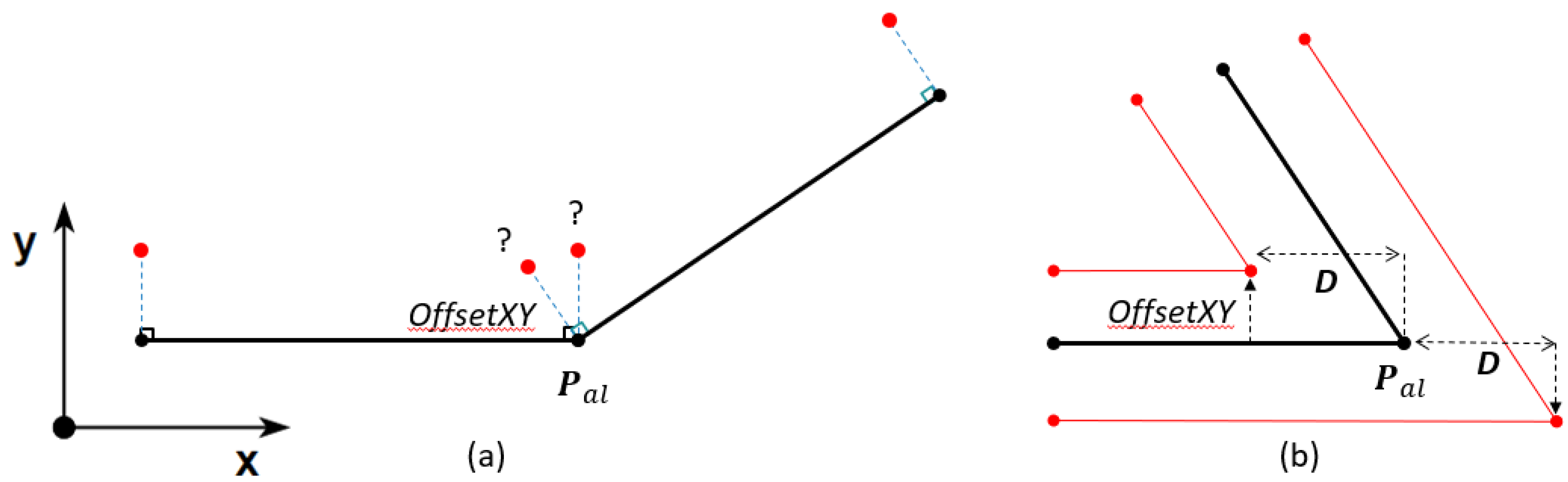
• OffsetXY: The perpendicular distance between each point in ${\mathit{P}}_{al}$ and each middle point of each road line.
• OffsetZ: The vertical distance between each point in ${\mathit{P}}_{al}$ and each middle point of each road line.
• Offset_id: Since there may be more than one lane per point in ${\mathit{P}}_{al}$, an index is stored for each pair of (OffsetXY, OffsetZ) that points to the coordinate in ${\mathit{P}}_{al}$ from which the offsets were obtained, allowing the offset alignment generation as explained in Section 2.2.6.

Figure 11 shows the results of this module. The road alignment, as well as the middle point of each road lane, are described as a set of ordered points with a small resolution such that a polyline can be defined without introducing a relevant error, even when there is a certain curvature on the road.

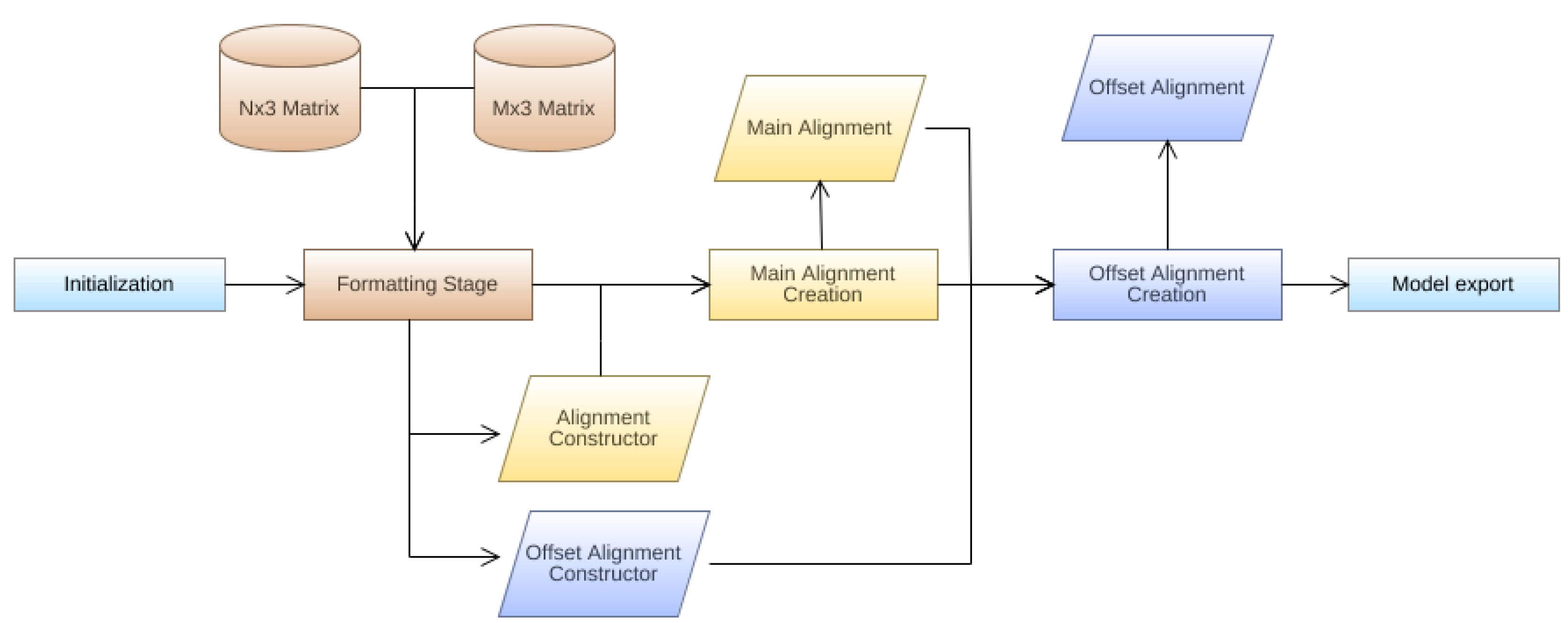
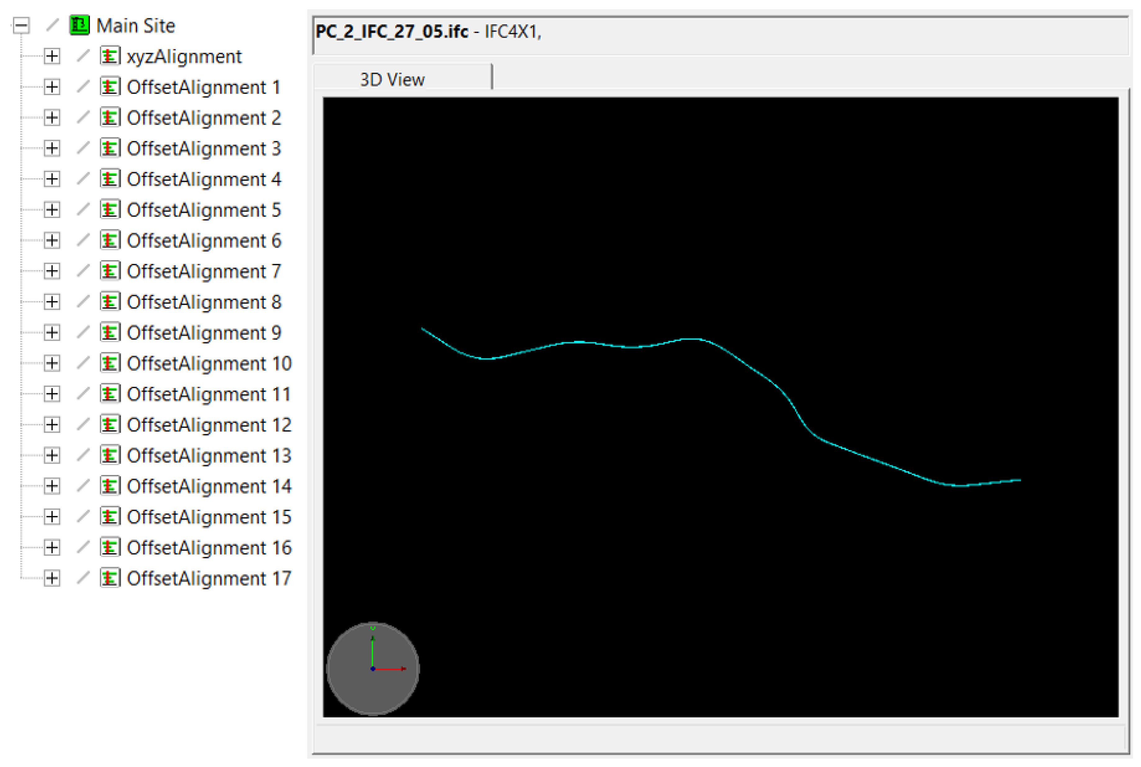
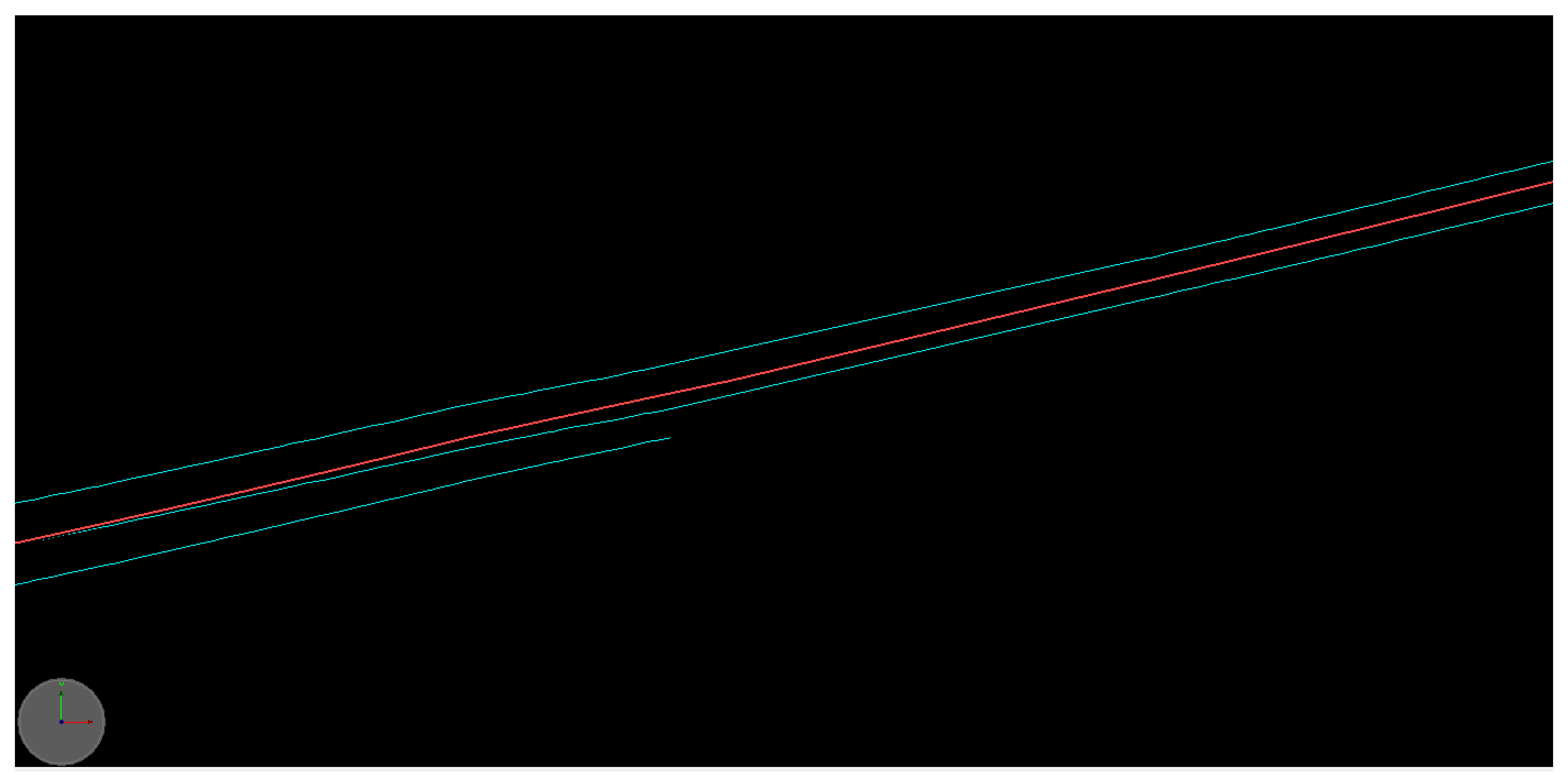
2.2.6. IFC Alignment Model Generation

The purpose of this module is to obtain an IFC model that contains the alignments for both the center of the road (main alignment) and the lanes (offset alignments).

To support the explanation of the procedure, both an UML class diagram and a general flowchart are provided to be understood along each other. The UML can be seen in Figure A1 (Appendix A) and the flowchart is visible in Figure 12.

The process revolves around an alignment hierarchy where the main alignment stands on top and the offset alignments depend on it for their geometry definition. While the nature of the hierarchy implies that the main alignment has to be created first, the process can be explained simultaneously, since the building process is quite similar. First, the data matrices obtained from the point cloud are fed into the system, where they are formatted into packages. These packages are called constructors and they contain the necessary information to define a unique curve. Depending on whether they describe the center of the road (MainAlignmentConstructor) or one of its lanes (OffsetAlignmentConstructor), the formatting varies, but the objective is the same: one constructor equals one curve. Then, these constructors are used to create segments describing the center of the road (IfcAlignment2DHorizontalSegment & IfcAlignment2DVerticalSegment), and offset points based on them that describe the shape of each lane (IfcDistanceExpression). Afterwards, the segments are concatenated forming the curve of the main alignment (IfcAlignmentCurve), and the points are connected forming the curves of the offset alignments (IfcOffsetCurveByDistances). Finally, these curves are used as the base for their corresponding IfcAlignment instances, and the model is exported into an IFC file.

For a more detailed explanation, the process can be broken down into its two stages: formatting the data, and creation of the alignments. As mentioned previously, the end goal of the formatting stage is to obtain one constructor for each curve. Additionally, it also serves to express the input data from the matrices (.csv) in an appropriate form, so that it can be easily used throughout the program. For the main alignment, this stage is a simple redistribution of the data found in the Nx3 matrix. This means that the constructor contains the coordinates of ${\mathit{P}}_{al}$ in an ordered list. However, for the offset alignments, the possibilities of incorporation lanes and missing data are also taken into account. The solution for both these issues is based on the Offset_id parameter. The Offset_id is an index that indicates to which main alignment point the accompanying OffsetXY and OffsetZ are related. Therefore, by querying all its values for repetition, a counter list is obtained. This counter list reflects the amount of times each index is repeated, indicating the number of lanes for each ${\mathit{P}}_{al}$. This allows the consideration of incorporation lanes, since the counter would increase in the moment a new lane appears, and decrease when it disappears. As for the missing data, if there is a jump in the sequential values of Offset_id (e.g., 1, 1, 2, 2, 15, 15, 16, 16), it means that there are no related OffsetXY and OffsetZ for the ${\mathit{P}}_{al}$ in between. To avoid misrepresenting that part of the road, the curves are split if the jump surpasses certain threshold. This implies that points before and after the split will belong to different curves and, therefore, to different constructors.

The creation stage for the main alignment is focused on the definition of linear segments connecting each sequential pair of ${\mathit{P}}_{al}$. Following the IFC schema, the vertical and horizontal components of the alignment are defined separately. Horizontal segments (IfcAlignment2DHorizontalSegment) contained in the XY-plane are described by their StartPoint, their SegmentLength, and their StartDirection. The StartPoint is given directly from ${\mathit{P}}_{al}$ and the SegmentLength is obtained as the norm of the vector connecting two consecutive ${\mathit{P}}_{al}$. The StartDirection is the counterclockwise angle of said vector, with respect to the x-axis. Vertical segments (IfcAlignment2DVerticalSegment), on the other hand, are defined based on their horizontal counterpart. Their description contains StartHeight, StartGradient, and HorizontalLength. As before, the StartHeight is given as the z coordinate of ${\mathit{P}}_{al}$. Their StartGradient is the slope, and the HorizontalLength is the same as the SegmentLength of their horizontal counterpart, since they are described for the same pair of ${\mathit{P}}_{al}$. These segments are then concatenated into the curve of the main alignment (IfcAlignmentCurve) and passed down for the creation of the offset alignments.

Modelling the offset alignment requires the consideration of the tangential discontinuity present when two consecutive segments of the main alignment have different StartDirection. This causes an angle difference between the segments, that translates into the issue depicted in Figure 13a. Because the point is between two segments with different perpendicular directions, it is not possible to directly place the OffsetXY measurement for that ${\mathit{P}}_{al}$. Furthermore, the angle difference also means that the lanes will be modeled differently from one another. Picture a smooth curve in a road, the interior lane has a different curvature radius than the exterior one, in order to keep the shape of the road. This effect is also translated when using line segments, the interior lane has to change direction sooner than the exterior lane. To do so, a shifting parameter D is calculated, whose purpose is to change the point in which the OffsetXY will be applied. This approach, seen in Figure 13b, solves both the discontinuity and this modelling issue. The perpendicular direction is obtained from the segment connecting to the target ${\mathit{P}}_{al}$. The point to apply the OffsetXY is then shifted backwards or projected forwards by D depending on whether it is an interior or exterior lane, respectively.

These points (IfcDistanceExpression) are then connected to form each of the offset alignment curves (IfcOffsetCurveByDistances). The final step is to use the curves obtained from the creation stage as the base for the IfcAlignment instances of the center of the road and the lanes. Finally, the model is exported as an IFC file.

3. Results

3.1. Parameters

In Section 2.2, several parameters and thresholds were introduced. In

Table 2. Values of the parameters used for the validation of the method.

Parameter	Value	Parameter	Value
$d_{\mu }$	0.05 m	$l_{roi}$	3.5 m
$d_{\sigma }$	0.05	${\alpha }_s$	10º
$bi{n}_l$	1 m	$soli{d}_{th2}$	20 m
$bi{n}_w$	0.15 m	$t_l$	0.75 m
$w_g$	15	$t_w$	0.75 m
$w_{th}$	5	𝛼𝑡ℎ	15º
$n_s$	0.5	$d_{th}$	50 m
$r_s$	0.2 m	$R{2}_{min}$	0.999
$ec{c}_{th}$	0.98	$d_{sample}$	1 m
$das{h}_{th}$	0.5 m	$bi{n}_{w2}$	0.5 m
$soli{d}_{th}$	7.5 m	$d_{lane}$	100 m

, they are summarized together with the values used for the validation of the method. In most cases, the definition of the parameters comes from previous knowledge of the problem (e.g., the geometric properties of road markings), and an empirical verification that is needed in every methodology heavily based on heuristics as the one presented in this work.

3.2. Road Marking Detection and Processing

This section is focused on the validation of the methods from Section 2.2.2 and Section 2.2.3 for road marking detection and processing respectively. Ground truth data were obtained by randomly selecting a 20% of the point cloud sections ${\mathit{𝓟}}_{gi}$ generated during the process and labelling them manually. This results in approximately 4 km of road that is used for validation. To simplify the labelling process for the manual operator, the point clouds were rasterized with a raster size of 0.1 m, and a pixel-wise labelling was carried out over the intensity image of the raster structure. To obtain validation results for road marking processing, two different classes are annotated: solid line and dashed line (Figure 14a).

Road marking detection is validated by directly comparing, pixel by pixel, the manually annotated images with the corresponding raster images that include the road markings from ${\mathit{𝓟}}_{mk}$ as defined in Section 2.2.2. The metrics used for this validation are Precision, Recall, and F-score (Equations (1)–(3)).

$$Precision=\frac{TP}{TP+FP}$$

(1)

$$Recall=\frac{TP}{TP+FP}$$

(2)

$$Fscore=\frac{2\ast Precision\ast Recall}{Precision+Recall}$$

(3)

where TP, FP, and FN are the number of true positive, false positive and false negative pixels respectively.

Furthermore, two distance metrics are considered to offer a better insight on the value of the validation metrics: $d_{FP}$ is the average distance, across the ground truth, between false positive points and their closer true positive points. Similarly, $d_{FN}$ is the average distance between false negative points and their closer true positive points. These distances allow to quantify the influence of the labelling quality on the results; a closer distance to the raster size implies a bigger influence of boundary errors on the labelling process. The results can be seen in

Table 3. Road marking detection results and validation metrics.

Precision	Recall	F-score	${\mathit{d}}_{\mathit{F}\mathit{p}}\left(\mathbf{m}\right)$	${\mathit{d}}_{\mathit{F}\mathit{N}}\left(\mathbf{m}\right)$
0.919	0.964	0.932	0.184	0.333

.

For road marking processing, a confusion matrix of solid and dashed lines across the ground truth is shown in

Table 4. Confusion matrix for road marking classification.

GT/Prediction	Solid Line	Dashed Line
Solid Line	99826	163
Dashed Line	466	13805

.

As it can be seen, the metrics for road marking detection are promising. Even if there exist false positives and false negatives in the validation data, most of them are in the boundaries of the markings (Figure 14b), which is reasonable as the manual labelling was done pixel-wise in intensity-based images with a resolution of 0.1 m.

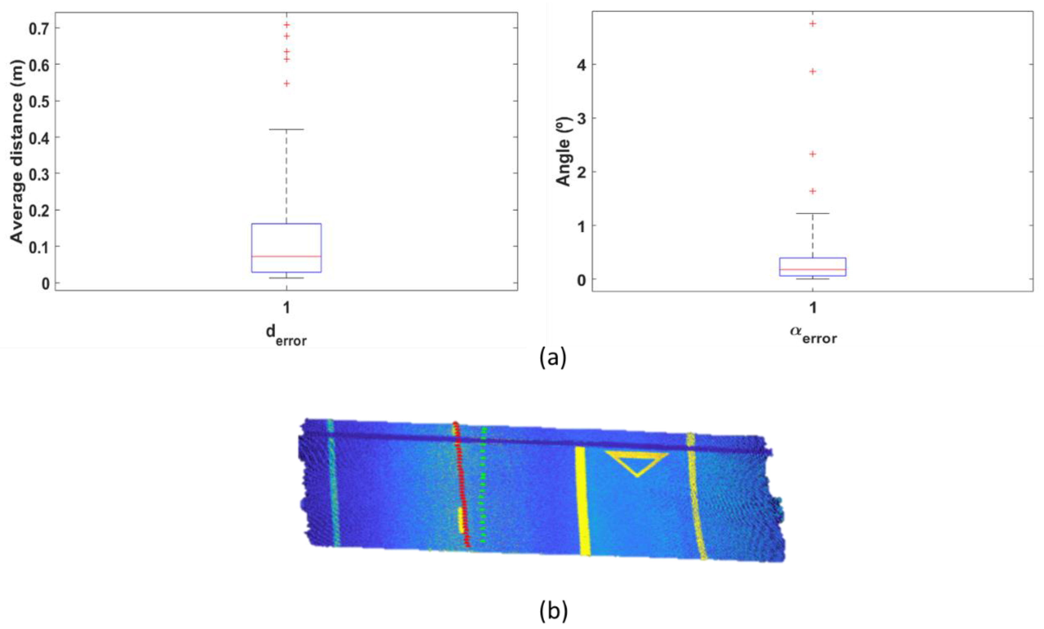
3.3. Alignment and Road Lane Processing

This section is focused on the validation of the methods from Section 2.2.5. The output of the point cloud processing modules is a set of ordered point coordinates that represent the alignment, or central line, of the road ($P_{al}$). Such set of points can be validated against manual references. A similar approach than in Section 3.2 was carried out, selecting a 20% of the sections ${\mathit{𝓟}}_{gi}$ randomly (this selection is independent from the one in Section 3.2), and manually defining a line on a raster image of the section that represents the alignment. The 3D line corresponding to the pixels selected by the manual annotation are retrieved, and two parameters are computed: the average distance of the points in $P_{al}$ corresponding to the section ${\mathit{𝓟}}_{gi}$ with respect to the reference 3D line ($d_{error}$) and the angle between the principal component of the points in $P_{al}$ and the director vector of the reference 3D line (${\alpha }_{error}$).

The results for all selected ${\mathit{𝓟}}_{gi}$ can be visually interpreted with the box plots in Figure 15a. The central mark of each box represents the median, which is 0.072 m for $d_{error}$ and 0.177º for ${\alpha }_{error}$. The top edge of the box indicates the 75th percentile, hence it can be seen that errors are small and close to the resolution of the images used for defining the ground truth. A few outliers are also present in the results. One of them is shown in Figure 15b, where the transition to a third lane which appears in the boundary of the section is not captured by the manual annotation.

Finally, Figure 16 shows a visualization of the alignment on Google Earth. The small error found in the validation data can be qualitatively generalized to the entire dataset given the visual results over the satellite image.

3.4. IFC Alignment Model Generation

The methodology employed in the IFC alignment model generation was explained in Section 2.2.6, using the UML class diagram present in Figure A1 (Appendix A) as a guide. It is based on the IFC 4.1 version of the schema and programmed using the xBIM 5.1.274 toolkit available for Visual Studio. However, while IFC 4.3 Draft Schema introduced several changes in the entity hierarchy and introduced new definitions, the geometric description of IfcAlignmentCurve and IfcOffsetCurveByDistances remained the same. Therefore, the alignment creation procedure showcased is valid for the newly released IFC 4.3. The exported IFC contains 17 offset alignments, as a result of the splitting procedure, to avoid missrepresentation of the road because of missing data. Their instances can be seen alongside the top view of the model in Figure 17.

Because of the scale of the road compared to the separation between the road lanes, it is necessary to zoom into an specific section to appreciate both the splits and lanes. Figure 18 shows several scenarios at once: (i) separation and paralelism between the lanes and main alignment; (ii) the appearance of a new lane; (iii) the reposition of the lanes to maintain the main alignment in the middle.

Overall, the shape of the road lanes followed the main alignment without any issues, mainly because of the thorough point cloud preprocessing. For reference, the viewer used through the development of the procedure and for the obtainment of the figures presented was FZK Viewer 5.3.1. Nevertheless, the obtained IFC model is merely a skeleton for future works following the IFC 4.3 release. The body of the road can be built upon the alignments given by this procedure, and semantic properties can be added to further enrich the model. While some of these steps would require a manual input or a new data feed, the existence of the alignments ease the introduction of these future lines of work.

4. Discussion

Attending to the results shown in Section 3, the proposed methodology is able to fulfill the objective and contributions of this work as presented in Section 1. First, the point cloud processing workflow outputs the main alignment and offset alignment of a highway road in a format that can be easily converted to an IFC compliant file. The validation of both road markings and alignment processing show a good performance in terms of errors with respect to manual references and has into consideration highway entrances and exits to define the alignment as the centerline of the road. Conversely, it can be argued that the main drawback of this method is the fact that it is not a fully automated process. This may have an impact on the time consumption of the method. Specifically, for Road Edge Detection (Section 2.2.4), manual corrections were required only for 20% of the point cloud sections of the case study but represent more than 65% of the total time of the process. Hence, it is clear that full automated and reliable processes would save resources in terms of time and manual interaction. Although full automation is a future objective for this research line, having a manual verification of the results before converting them to an IFC file guarantees the final user that any relevant error on the point cloud processing stage is corrected beforehand. Another future line of research will be motivated by the large number of heuristics that are defined throughout the point cloud processing workflow. With a larger amount of labelled data, it should be possible to train supervised learning algorithms and set classification models that allow road marking classification with no need of manual parameter tuning.

Second, a UML diagram that defines the construction of the IFC file is proposed (Appendix A). The generation of IFC compliant files from point cloud data of road infrastructure is expected to be a relevant research field in the next few years with the newly released IFC 4.3, where the definition of IfcAlignment objects will be essential for the positioning of the different road elements. Furthermore, different infrastructures could be interconnected (railways, bridges, etc.,) as a result of the harmonization process that is at the core of IFC 4.3. As the standardization process evolves, different civil engineering software tools are expected to be able to work with IFC files, hence the interest and potential of point cloud processing tools that allow the generation of this type of information models. Similar processes that allow to define IFC-compliant infrastructure entities are a natural future line for this research, once standards such as IFC Road are published and openly available. The feasibility of this line of research is being demonstrated in recent work [31,32]. Nevertheless, the automatic generation of an IFC model containing the alignments should be viewed as an alternative form of presenting information. This means that the point cloud is to be cleaned and preprocessed before passing it down to create an IFC-based model. Therefore, it is completely dependent on the raw data provided. If the input data are refined and set to describe a smooth curve, it will be reflected in the outcome of the IFC as well. The major drawback of the procedure on itself is that it uses an average number of lanes as basis. This assists the modeling of appearing lanes, but it would present issues if the number were to drop below that average on a section of the road. Regardless of this, the process has automatically created alignments that describe 20 km of road and, while the techniques are to be refined as a future line of work, it can be seen as a baseline for modelling the road itself, now that IFC 4.3 has been released.

5. Conclusions

This paper presents a methodology that outputs IFC-compliant files that model the alignment and the centerline of the road lanes of a highway road, using point cloud data that is processed in a semi-automated manner (automatic processing with manual validation) as input. The point cloud processing framework includes methods for ground segmentation, road marking detection and extraction, road edge detection based on the road markings, and finally alignment and road lane processing. In order to validate the methodology, information extracted from both road markings and alignment are compared with manual references, showing state-of-the-art performance for road marking processing and average errors close to the resolution of the reference for the alignment.

This Cloud-to-IFC workflow is expected to generate interest in infrastructure owners and administrations as BIM projects in infrastructure start to be more common, and buildingSMART just released IFC 4.3 as the result of the harmonization procedure between different infrastructure domains. Future research would consider expanding the alignment description to include arc segments and transition curves, modelling the assets covered by the schema beyond their alignment, and exploring the capabilities of remote sensing data to assist the generation of information models of built infrastructure.

References

1. Borrmann, A.; König, M.; Koch, C.; Beetz, J. Building Information Modeling: Technology Foundations and Industry Practice; Springer: Berlin, Germany, 2018; ISBN 9783319928623. [Google Scholar]
2. Costin, A.; Adibfar, A.; Hu, H.; Chen, S.S. Building Information Modeling (BIM) for transportation infrastructure–Literature review, applications, challenges, and recommendations. Autom. Constr. 2018, 94, 257–281. [Google Scholar] [CrossRef]
3. Chong, H.Y.; Lopez, R.; Wang, J.; Wang, X.; Zhao, Z. Comparative analysis on the adoption and use of BIM in Road infrastructure projects. J. Manag. Eng. 2016, 32, 05016021. [Google Scholar] [CrossRef]
4. Bradley, A.; Li, H.; Lark, R.; Dunn, S. BIM for infrastructure: An overall review and constructor perspective. Autom. Constr. 2016, 71, 139–152. [Google Scholar] [CrossRef]
5. IFC Release Notes–building SMART Technical. Available online: https://technical.buildingsmart.org/standards/ifc/ifc-schema-specifications/ifc-release-notes/ (accessed on 17 July 2020).
6. Pătrăucean, V.; Armeni, I.; Nahangi, M.; Yeung, J.; Brilakis, I.; Haas, C. State of research in automatic as-built modelling. Adv. Eng. Inform. 2015, 29, 162–171. [Google Scholar] [CrossRef] [Green Version]
7. Sacks, R.; Kedar, A.; Borrmann, A.; Ma, L.; Brilakis, I.; Hüthwohl, P.; Daum, S.; Kattel, U.; Yosef, R.; Liebich, T.; et al. SeeBridge as next generation bridge inspection: Overview, information delivery manual and model view definition. Autom. Constr. 2018, 90, 134–145. [Google Scholar] [CrossRef] [Green Version]
8. Guan, H.; Li, J.; Cao, S.; Yu, Y. Use of mobile LiDAR in road information inventory: A review. Int. J. Image Data Fusion 2016, 7, 219–242. [Google Scholar] [CrossRef]
9. Gargoum, S.A.; El-Basyouny, K. Automated extraction of road features using LiDAR data: A review of LiDAR applications in transportation. In Proceedings of the 2017 4th International Conference on Transportation Information and Safety (ICTIS), Baniff, AB, Canada, 8–10 August 2017; Institute of Electrical and Electronics Engineers (IEEE): Piscataway, NJ, USA, 2017; pp. 563–574. [Google Scholar]
10. Ma, L.; Li, Y.; Li, J.; Wang, C.; Wang, R.; Chapman, M.A. Mobile laser scanned point-clouds for road object detection and extraction: A review. Remote Sens. 2018, 10, 1–33. [Google Scholar] [CrossRef] [Green Version]
11. Soilán, M.; Sánchez-Rodríguez, A.; Del Río-Barral, P.; Perez-Collazo, C.; Arias, P.; Riveiro, B.; Rodríguez, S.; Barral, R.; Collazo, P. Review of laser scanning technologies and their applications for road and railway infrastructure monitoring. Infrastructures 2019, 4, 58. [Google Scholar] [CrossRef] [Green Version]
12. Arcos-García, Á.; Soilán, M.; Álvarez-García, J.A.; Riveiro, B. Exploiting synergies of mobile mapping sensors and deep learning for traffic sign recognition systems. Expert Syst. Appl. 2017, 89, 286–295. [Google Scholar] [CrossRef]
13. Yu, Y.; Li, J.; Wen, C.; Guan, H.; Luo, H.; Wang, C. Bag-of-visual-phrases and hierarchical deep models for traffic sign detection and recognition in mobile laser scanning data. ISPRS J. Photogramm. Remote Sens. 2016, 113, 106–123. [Google Scholar] [CrossRef]
14. Ai, C.; Tsai, Y.C. An automated sign retroreflectivity condition evaluation methodology using mobile LIDAR and computer vision. Transp. Res. Part C Emerg. Technol. 2016, 63, 96–113. [Google Scholar] [CrossRef]
15. Zhang, S.; Wang, C.; Lin, L.; Wen, C.; Yang, C.; Zhang, Z.; Li, J. Automated visual recognizability evaluation of traffic sign based on 3D LiDAR point clouds. Remote Sens. 2019, 11, 1453. [Google Scholar] [CrossRef] [Green Version]
16. Novo, A.; González-Jorge, H.; Martínez-Sánchez, J.; González-De Santos, L.M.; Lorenzo, H. Automatic detection of forest-road distances to improve clearing operations in road management. In Proceedings of the International Archives of the Photogrammetry, Remote Sensing and Spatial Information Sciences. ISPRS Geospatial Week, Enschede, The Netherlands, 10–14 June 2019; pp. 1083–1088. [Google Scholar]
17. Novo, A.; González-Jorge, H.; Martínez-Sánchez, J.; Lorenzo, H. Canopy detection over roads using mobile lidar data. Int. J. Remote Sens. 2019, 41, 1927–1942. [Google Scholar] [CrossRef]
18. Zou, X.; Cheng, M.; Wang, C.; Xia, Y.; Li, J. Tree classification in complex forest point clouds based on deep learning. IEEE Geosci. Remote Sens. Lett. 2017, 14, 2360–2364. [Google Scholar] [CrossRef]
19. Yu, Y.; Li, J.; Guan, H.; Wang, C.; Wen, C. Bag of contextual-visual words for road scene object detection from mobile laser scanning data. IEEE Trans. Intell. Transp. Syst. 2016, 17, 3391–3406. [Google Scholar] [CrossRef]
20. Luo, H.; Wang, C.; Wen, C.; Cai, Z.; Chen, Z.; Wang, H.; Yu, Y.; Li, J. Patch-based semantic labeling of road scene using colorized mobile LiDAR point clouds. IEEE Trans. Intell. Transp. Syst. 2015, 17, 1286–1297. [Google Scholar] [CrossRef]
21. Yu, Y.; Li, J.; Guan, H.; Jia, F.; Wang, C. Learning hierarchical features for automated extraction of road markings from 3-D mobile LiDAR point clouds. IEEE J. Sel. Top. Appl. Earth Obs. Remote Sens. 2014, 8, 709–726. [Google Scholar] [CrossRef]
22. Guan, H.; Li, J.; Yu, Y.; Ji, Z.; Wang, C. Using mobile LiDAR data for rapidly updating road markings. IEEE Trans. Intell. Transp. Syst. 2015, 16, 2457–2466. [Google Scholar] [CrossRef]
23. Soilán, M.; Riveiro, B.; Martínez-Sánchez, J.; Arias, P. Segmentation and classification of road markings using MLS data. ISPRS J. Photogramm. Remote Sens. 2017, 123, 94–103. [Google Scholar] [CrossRef]
24. Wen, C.; Sun, X.; Li, J.; Wang, C.; Guo, Y.; Habib, A. A deep learning framework for road marking extraction, classification and completion from mobile laser scanning point clouds. ISPRS J. Photogramm. Remote Sens. 2019, 147, 178–192. [Google Scholar] [CrossRef]
25. Zhao, H. Recognizing Features in Mobile Laser Scanning Point Clouds Towards 3D High-definition Road Maps for Autonomous Vehicles. Master’s Thesis, University of Waterloo, Waterloo, ON, Canada, 2017. [Google Scholar]
26. Ye, C.; Li, J.; Jiang, H.; Zhao, H.; Ma, L.; Chapman, M. Semi-automated generation of road transition lines using mobile laser scanning data. IEEE Trans. Intell. Transp. Syst. 2020, 21, 1877–1890. [Google Scholar] [CrossRef]
27. Puente, I.; González-Jorge, H.; Riveiro, B.; Arias, P. Accuracy verification of the Lynx Mobile Mapper system. Opt. Laser Technol. 2013, 45, 578–586. [Google Scholar] [CrossRef]
28. Douillard, B.; Underwood, J.; Kuntz, N.; Vlaskine, V.; Quadros, A.; Morton, P.; Frenkel, A. On the segmentation of 3D LIDAR point clouds. In Proceedings of the 2011 IEEE International Conference on Robotics and Automation, Shanghai, China, 9–13 May 2011; pp. 2798–2805. [Google Scholar] [CrossRef]
29. Otsu, N. Threshold selection method from grey-level histograms. IEEE Trans. Syst. Man. Cybern. 1979, 9, 62–66. [Google Scholar] [CrossRef] [Green Version]
30. Soilán, M.; Riveiro, B.; Martínez-Sánchez, J.; Arias, P. Traffic sign detection in MLS acquired point clouds for geometric and image-based semantic inventory. ISPRS J. Photogramm. Remote Sens. 2016, 114, 92–101. [Google Scholar] [CrossRef]
31. Barazzetti, L.; Previtali, M.; Scaioni, M. Roads detection and parametrization in integrated BIM-GIS using LiDAR. Infrastructures 2020, 5, 55. [Google Scholar] [CrossRef]
32. Liu, X.; Wang, X.; Wright, G.; Cheng, J.C.; Li, X.; Liu, R. A state-of-the-art review on the integration of building information modeling (BIM) and geographic information system (GIS). ISPRS Int. J. Geo-Inf. 2017, 6, 53. [Google Scholar] [CrossRef] [Green Version]
Figure 1. Case study data. (a) Optech LYNX Mobile Mapper. (b) Raw point cloud section.
Remotesensing 12 02301 g001
Figure 2. Workflow of the presented method.
Remotesensing 12 02301 g002
Figure 3. Ground segmentation. (a) Raw point cloud 𝓟 r a w ; (b) the segmented cloud 𝓟 g is colored in red
Remotesensing 12 02301 g003
Figure 4. The point cloud 𝓟 g is partitioned in several transversal sections with respect to the trajectory of the vehicle, with a certain overlap. Each section is subdivided in smaller bins to get a locally averaged intensity value.
Remotesensing 12 02301 g004
Figure 5. Road markings detection. (a) 3D point cloud employed to generate a single intensity profile. (b) Intensity profile, with normalized and filtered intensities. (c) Detected road markings on the 3D point cloud are colored in red.
Remotesensing 12 02301 g005
Figure 6. The result of road markings detection, 𝓟 m k , is colored in red over the point cloud.
Remotesensing 12 02301 g006
Figure 7. Road markings processing. (a) False negatives or occlusions on solid lines are corrected using a region growing method that follows the detected line. False positives are removed based on angle α t m (which has been exaggerated for better understanding of the figure) and length of the marking l m .   (b) Dashed markings are merged together based on angle α c d and distance d c d   false negatives can be found using parameter d a v g .   (c) Processed road markings are shown in the 3D point cloud (solid lines colored in red, dashed lines colored in green).
Remotesensing 12 02301 g007
Figure 8. Road edges are shown in the 3D point cloud, right edge 𝓟 r e in green and left edge 𝓟 l e in red.
Remotesensing 12 02301 g008
Figure 9. The alignment P a l is obtained from the sampled road edges.
Remotesensing 12 02301 g009
Figure 10. Road lane processing. (a) Example of a road section with two lanes. (b) Example of a road section with three lanes.
Remotesensing 12 02301 g010
Figure 11. The alignment (black points) and the centerline of each road line (which is employed to define the offset alignment -red and green points-) are shown in the 3D point cloud.
Remotesensing 12 02301 g011
Figure 12. General flowchart diagram of the Industry Foundation Classes (IFC) alignment model generation.
Remotesensing 12 02301 g012
Figure 13. Offset alignment modelling. (a) Unknown perpendicular direction. (b) Shifting parameter solution.
Remotesensing 12 02301 g013
Figure 14. Road markings processing results. (a) Manual reference with labels for solid and dashed lines. (b) False positives (red) and false negatives (black) are highlighted on the 3D point cloud.
Remotesensing 12 02301 g014
Figure 15. Alignment extraction results. (a) Box plots of the error metrics d e r r o r and α e r r o r . (b) Example of a road section that results in an outlier for d e r r o r due to the transition to a third road lane that appears in the boundary of the section, where manual reference is colored in red and alignment points are colored in green
Remotesensing 12 02301 g015
Figure 16. Points of P a l for the case study data displayed as a point layer on Google Earth.
Remotesensing 12 02301 g016
Figure 17. Top view of the IFC model and its alignment instances.
Remotesensing 12 02301 g017
Figure 18. Main alignment (reds) and offset alignments (blue). Third lane appearance.
Remotesensing 12 02301 g018