Article

Multi-Decadal Changes in Mangrove Extent, Age and Species in the Red River Estuaries of Viet Nam

1
Vietnam National Space Center (VNSC), Vietnam Academy of Science and Technology (VAST), 18 Hoang Quoc Viet, Hanoi 100000, Vietnam
2
Sustainability Research Institute, School of Earth and Environment, University of Leeds, Leeds LS2 9JT, UK
3
School of Geography, Politics and Sociology, Newcastle University, Newcastle upon Tyne NE1 7RU, UK
4
Central Institute for Natural Resources and Environmental Studies, Vietnam National University (VNU), No 19 Le Thanh Tong, Hoan Kiem, Ha Noi 100000, Vietnam
5
Faculty of Biology, Hanoi National University of Education (HNUE), 136 Xuan Thuy, Cau Giay, Ha Noi 100000, Vietnam
*
Author to whom correspondence should be addressed.
Remote Sens. 2020, 12(14), 2289; https://doi.org/10.3390/rs12142289
Submission received: 10 June 2020 / Revised: 3 July 2020 / Accepted: 14 July 2020 / Published: 16 July 2020
(This article belongs to the Special Issue Remote Sensing in Mangroves)

Abstract

:
This research investigated the performance of four different machine learning supervised image classifiers: artificial neural network (ANN), decision tree (DT), random forest (RF), and support vector machine (SVM) using SPOT-7 and Sentinel-1 images to classify mangrove age and species in 2019 in a Red River estuary, typical of others found in northern Viet Nam. The four classifiers were chosen because they are considered to have high accuracy, however, their use in mangrove age and species classifications has thus far been limited. A time-series of Landsat images from 1975 to 2019 was used to map mangrove extent changes using the unsupervised classification method of iterative self-organizing data analysis technique (ISODATA) and a comparison with accuracy of K-means classification, which found that mangrove extent has increased, despite a fall in the 1980s, indicating the success of mangrove plantation and forest protection efforts by local people in the study area. To evaluate the supervised image classifiers, 183 in situ training plots were assessed, 70% of them were used to train the supervised algorithms, with 30% of them employed to validate the results. In order to improve mangrove species separations, Gram–Schmidt and principal component analysis image fusion techniques were applied to generate better quality images. All supervised and unsupervised (2019) results of mangrove age, species, and extent were mapped and accuracy was evaluated. Confusion matrices were calculated showing that the classified layers agreed with the ground-truth data where most producer and user accuracies were greater than 80%. The overall accuracy and Kappa coefficients (around 0.9) indicated that the image classifications were very good. The test showed that SVM was the most accurate, followed by DT, ANN, and RF in this case study. The changes in mangrove extent identified in this study and the methods tested for using remotely sensed data will be valuable to monitoring and evaluation assessments of mangrove plantation projects.

Graphical Abstract

1. Introductions

Mangrove forests are one of the most biologically diverse ecosystems on Earth and deliver numerous provisioning, regulating, cultural, and supporting services that benefit the coastal and inland communities’ livelihoods as well as the global atmospheric commons [1,2]. The Vietnamese government, aware of these benefits, has developed strategies for mangrove development in the Red River Delta (RRD), in order to reduce global climate change impacts and secure the livelihoods of coastal communities in the five coastal provinces in the north of the country [3]. One of the key strategies is forest plantation and restoration, involving both domestic and foreign donors (such as Denmark and Japan). Although some mangrove areas have been converted for use in aquaculture, rice, and salt farms, there has been an expansion of the mangrove forest in recent decades in some Red River estuarine areas, for example, mangrove extent increased by 538.5-ha in Thuy Truong commune between 2001 and 2016 [4]. However, there is a need for information regarding forest dynamics in terms of area cover as well as accurate methods for mapping the extent and composition of these forests with contemporary remote sensing data and methods. Compositional factors are linked to a number of variables such as size class distribution and canopy complexity, that when used in combination with others can be indicative of mangrove health or condition [5]. Therefore, understanding them can provide useful insights to support future forest management decision making.
In recent years, supervised image classification algorithms have been reported to be more accurate than unsupervised approaches [6], as the supervised outputs are trained with in situ data. Without ground-truth data, the supervised classifiers should not be applied because a minimum training dataset is required consistently [7]. However, training datasets are not always available, particularly when historic image analysis is undertaken [8]. In this paper, we applied qualified unsupervised classifiers, the iterative self-organizing data analysis technique (ISODATA) and the K-means classification, to analyze a long time series of Landsat-X data for an assessment of changes in mangrove extent. In addition, field-surveyed data were obtained to test four different learning machine image classifiers: artificial neural network (ANN), decision tree (DT), random forest (RF), and support vector machine (SVM) in order to classify mangrove age and species at a point in time of May 2019.
In the present era of digital image processing, the image fusion of multisource remote sensing data is of increasing interest and is becoming a well-established research field in the context of increasing (optical and synthetic aperture radar (SAR)) data availability [9,10]. Image fusion techniques are applied to sharpen a low resolution multispectral image using a higher resolution panchromatic layer to generate enhanced input data, resulting in new, better quality data (spectral and spatial resolution) compared to the originals [11,12]. However, sometimes it is difficult to preserve the original image spectrum. In addition, spectral distortion due to image fusion effects is a source of new information that can be used for other applications such as change detection [13]. Recently, the number of studies integrating SAR and optical images has increased as users take advantage of both of these data. Several methods of image fusion have been developed, hence the decision about which technique is the most suitable is driven by the study goals [14] and expected accuracy requirement. Here, we selected Gram–Schmidt (GS), and principal component analysis (PCA), a method which reduces the dimensionality of the information present in the original multi-band dataset, as they have been reported to be the most accurate methods [15] when fusing SPOT-7 and Sentinel-1 images, with the expectation of achieving improved mangrove species classification [16].
Remote sensing has undoubtedly been an effective tool to evaluate mangrove forests from many perspectives [17] including estimating above ground biomass [18,19,20,21], assessing mangrove health [22,23,24], chlorophyll [25,26], and to map changes in mangrove extent [27,28] at global [29], continental and regional [30,31], and national and smaller scales [32,33]. Most studies use remote sensing to explore the severity and consequences of mangrove loss and associated degradation. In this study, we applied three sources of remote sensing data to better understand elements of mangrove condition related to growth as well as to test the performance of different classification approaches.

2. Materials and Methods

2.1. Study Site

Mangroves and coastal wetland areas are described in [34]. Vietnam has 30 coastal provinces and cities associated with mangroves divided into four main zones: (i) Northeastern coast (Ngoc Cape to Do Son); (ii) Northern Delta (Do Son to Lach Truong River); (iii) Central coast (Lach Truong to Vung Tau); and (iv) Southern Delta (Vung Tau to Ha Tien) [4]. Our study is located in Thuy Truong commune, which is located in the Northern Delta (zone 2) at the mouth of the Thai Binh River (Figure 1A). The climate of the region is influenced by the South-East Asian tropical monsoon with four distinct seasons: spring from February to May, summer from June to August, autumn from September to November, and winter from December to January. The mean annual temperature is 23 °C and maximum and minimum monthly average temperatures are around 28 °C in July and 16 °C in January, respectively [35]. The area of Thuy Truong commune is 9.3 km2 and home to 10,000 people. The main livelihoods are based on agriculture (rice cultivation and cash crops), aquaculture, and harvesting clams, fishes, and crabs in the nearby mangrove forests [36]. The mangrove forest has been expanded as a result of plantation efforts supported by the Danish and Japanese Red Cross programs that ended in 2006 [37]. Hence, although Vietnam’s total mangrove area has declined to 62% of the original [38], in Thuy Truong, the mangrove forest has been subject to large fluctuations in extent and quality [39].

2.2. Data Collection

2.2.1. Ground-Truth Data Collection

Field investigations from 22 to 25 November 2018 were undertaken to obtain ground-truth information including 78 polygons for training mangrove species (23 polygons for accuracy assessment) and 105 polygons for training mangrove age (32 polygons for accuracy assessment). The number of samples for each class is summarized in Table 1. It was noted that later image classifications focused on the mangrove forest, however, we also needed to train other land use and land cover (LULC) layers that help to discriminate mangroves and improve the accuracy of classification algorithms. We interviewed a commune cadastral official for the mangrove plantation projects and conducted field work with five local citizens to gather mangrove age and species information and mark them on a printed map. Mangroves have been present in the study site for about 45 years, since 1975, however trees older than 10 years are all similar in terms of height, stems and color. Hence, we divided mangrove age into three categories: older than 10 years, around five years, and under three years old. Despite the original plantation projects spanning a larger area, most of the planted mangrove had been destroyed by waves, erosion, or eaten by crabs and clams.

2.2.2. Remote Sensing Data
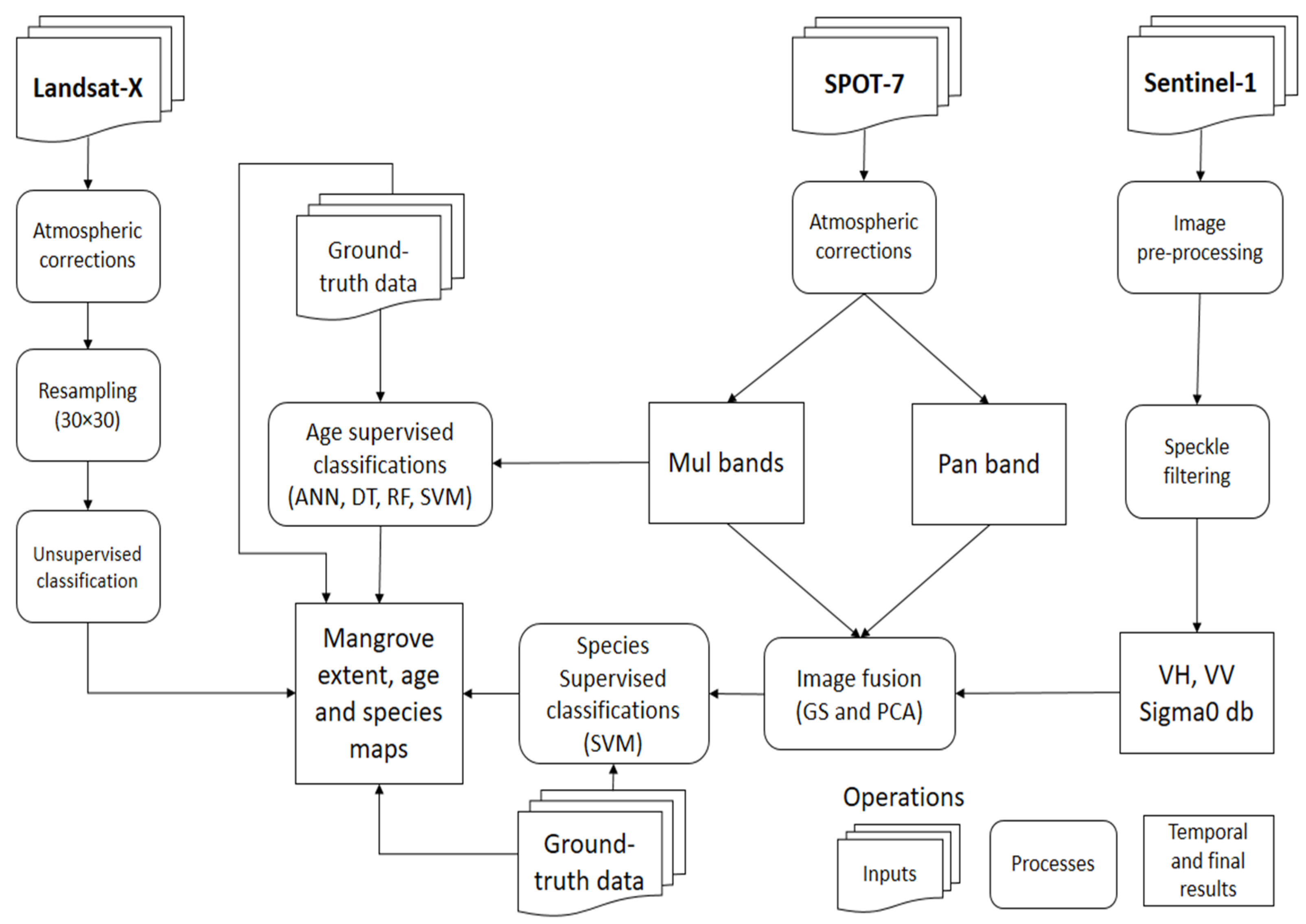
Landsat-2,5 and 8, SPOT-7, and Sentinel-1 datasets were used for this research, first, to compare extracted mangrove results, and second, to fuse the optical multi-spectral and panchromatic bands with SAR backscatter bands in the Sentinel-1 data. The basic information of acquisition time, processing level, band number, and spatial resolution of the collected scenes is summarized in Table 2. The Landsat data were acquired for each 5-year period from 1975 to 2019, and with the exception of Landsat-2 data for which there were limited options, and acquisition times for the Landsat scenes were selected to minimize cloud cover (October and November). To minimize seasonal effects, the acquisition date of Landsat-8 data was chosen to be as close as possible to the acquisition date of the SPOT-7 and the Sentinel-1 images to facilitate later comparisons. The high-resolution optical remote sensing scene of SPOT-7 consisted of four multispectral bands (0–3) and one panchromatic band with 1.6 m spatial resolution. The SAR image of Sentinel-1 was processed at the ground-range detected level (10 m resolution), was pass ascending, and acquired in two polarizations (VH and VV). Sentinel-1 data were obtained from the Copernicus Open Access Hub website of European Space Agency (ESA), Landsat scenes from the United States Geological Survey (USGS), and SPOT-7 data from the Airbus group.

2.3. Methodology

Figure 2 sets out our working flow chart, which comprises three main parts: (1) The processes for the Landsat-X mangrove extent unsupervised classification; (2) the procedures to process the SPOT-7 image to classify mangrove age and fusion with the Sentinel-1 images; and (3) the processing chain including image pre-processing, speckle filtering, fusing of the VH and VV layers with the SPOT-7 image, and supervised classification of mangrove types. Minor steps such as clipping the region of interest, post-classification to convert the classified image to vector, confusion matrix (contingency matrix) calculation, band math, band conversion, etc. are not included in order to simplify the figure. Basic tasks in remote sensing image processing, like atmospheric correction [40,41], image resampling (done only for Landsat-2), SAR image pre-processing (radiometric calibration, terrain correction, and data conversion/select band to export single layer) and speckle filtering are well documented [42,43], hence they are not described in detail here. The core tasks of classifying mangrove extent, age, and species, and image fusion are explained in the following sub-sections.

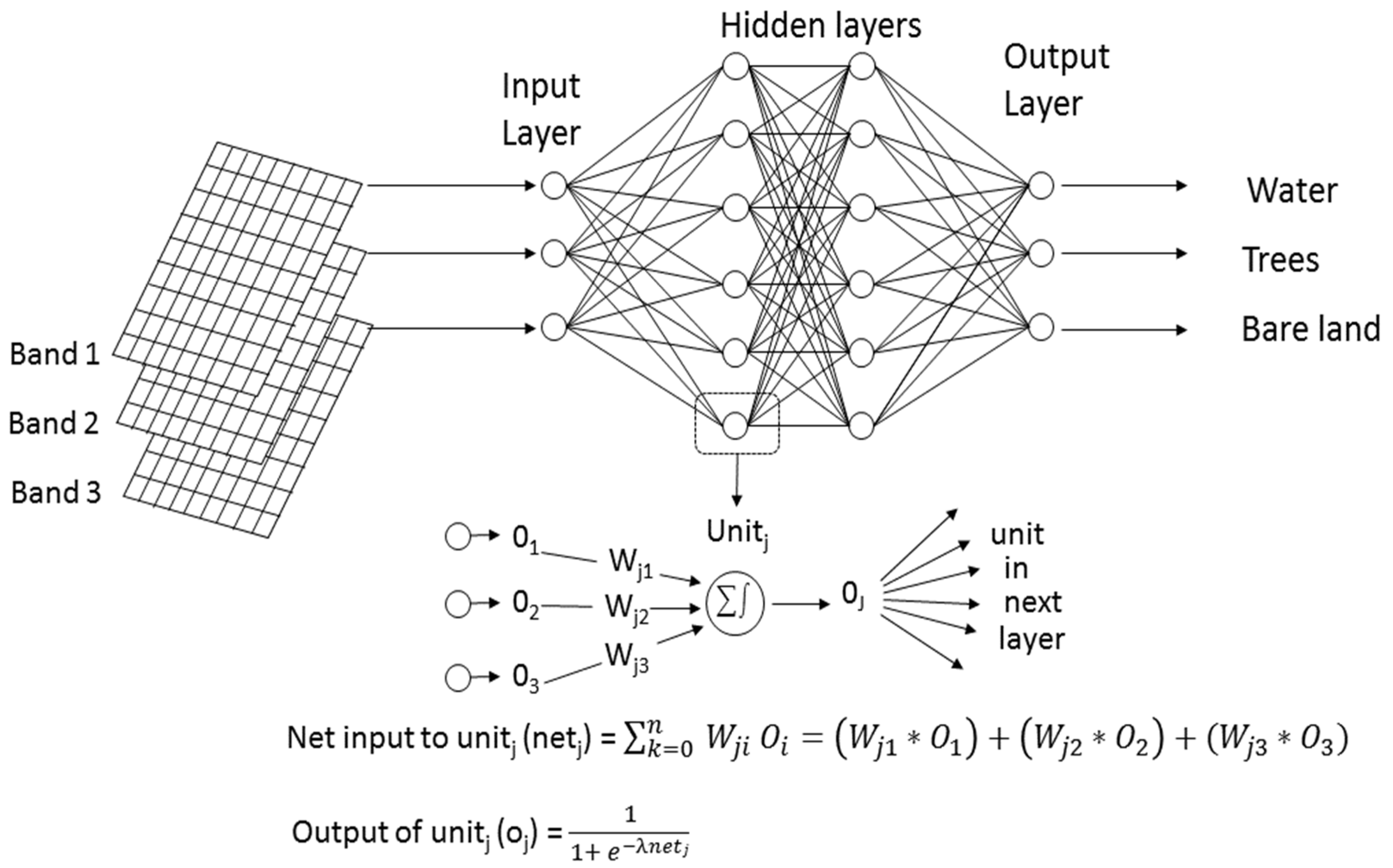
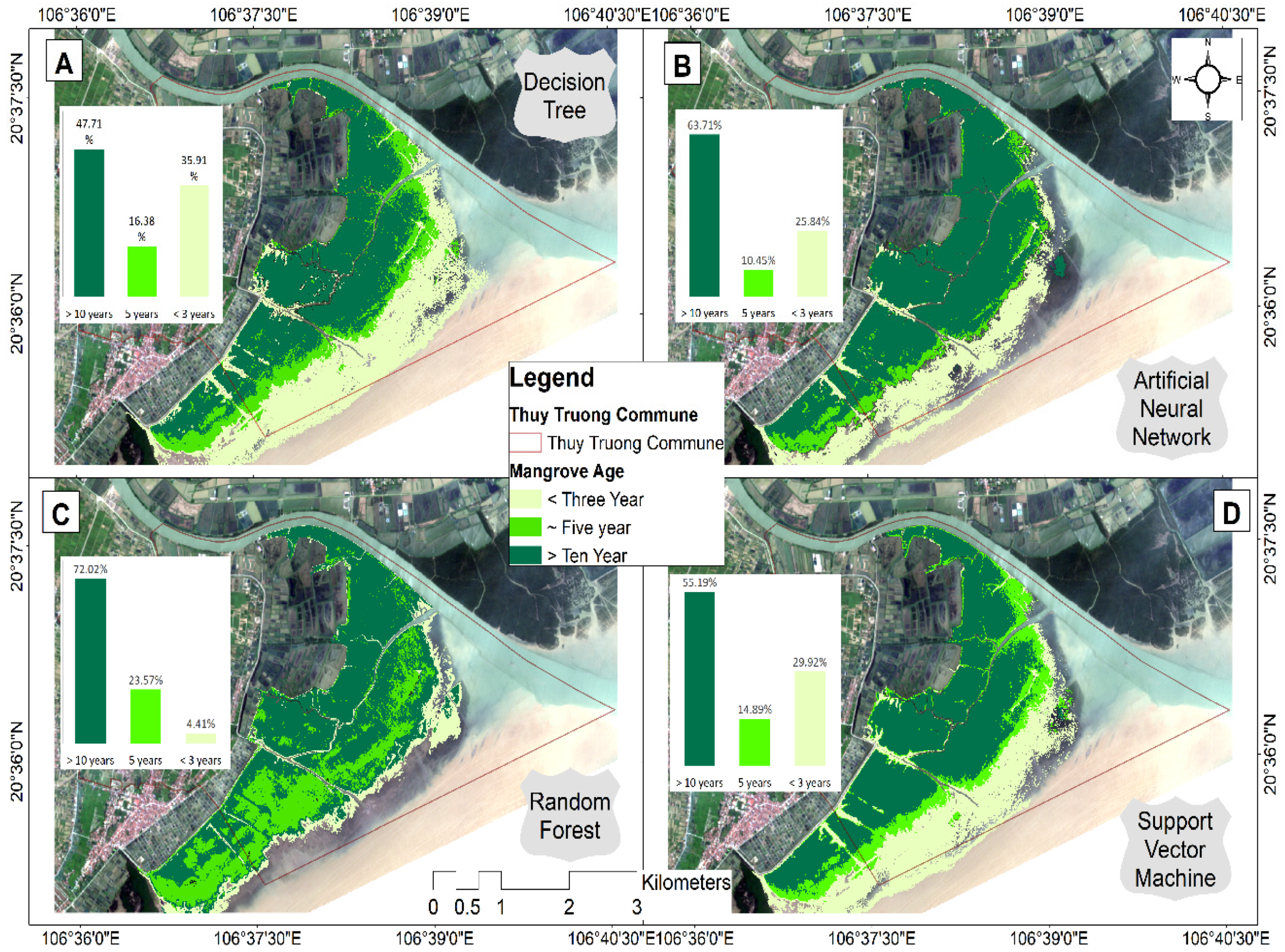
2.3.1. Mangrove Age Classification
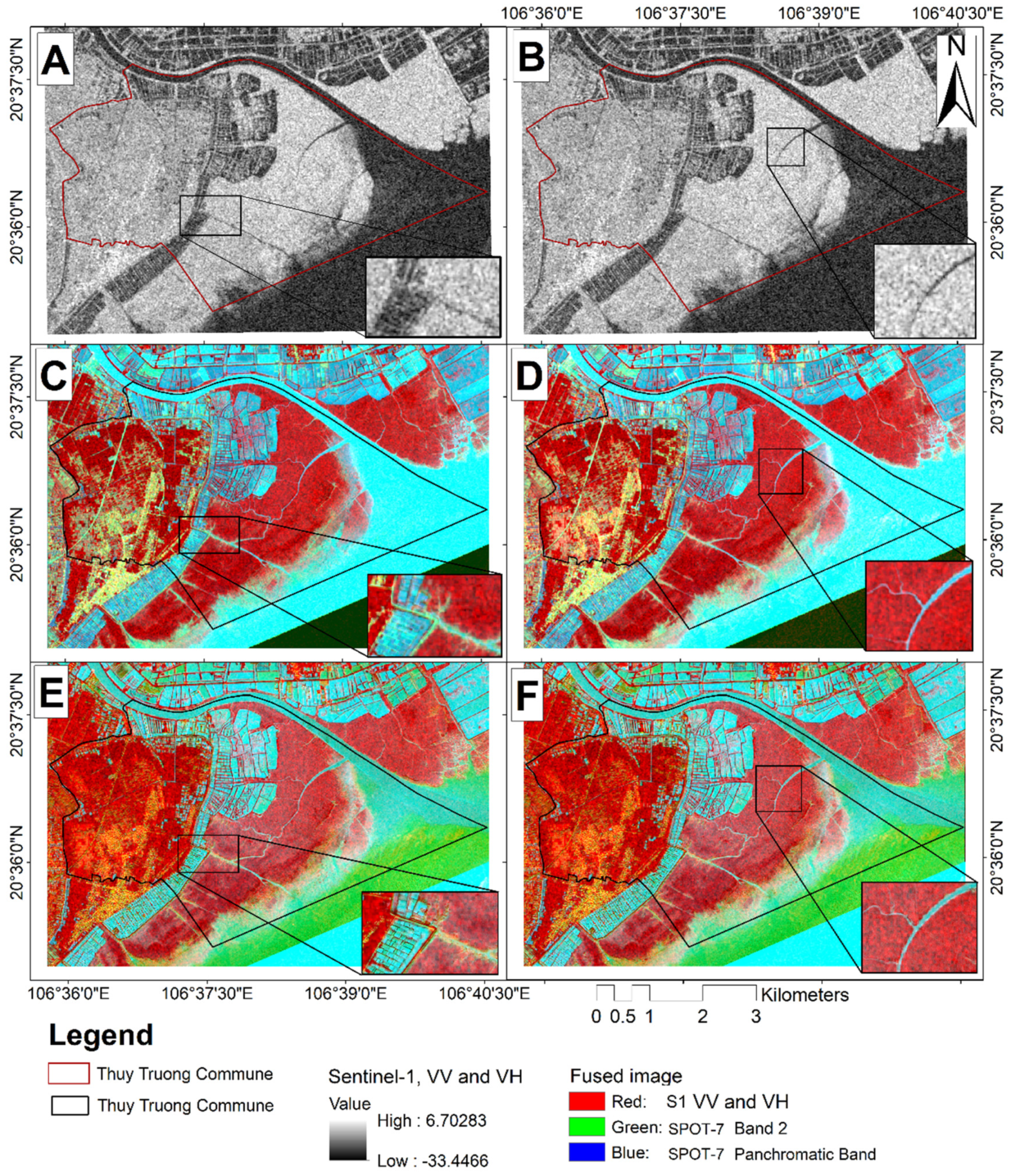
Mangrove age and growth estimations are typically quantified by means of in situ dendrometer techniques [44] and internodes [45]. However, few studies have attempted to define classifiers dealing with mangrove age estimations from remotely sensed data. We elected to use artificial neural network (ANN), decision tree (DT), random forest (RF), and support vector machine (SVM) methods from among the many available for the mangrove age estimation because (1) they are robust image supervised classification methods; (2) the advancements in machine learning (ML) approaches to model complex class signatures and accept a variety of training data [46]; and (3) because they are routinely found to have higher accuracies than the maximum likelihood method [47]. Selection of these four methods allowed us to compare results and identify the best performing method using the SPOT-7 image and the same training dataset from the field survey (Section 2.2.1).
ANN classification has been used in a wide range of applications in remote sensing. The theory and algorithm are explained in detail by Schalkoff (1992), Foody (1996), and Dreiseitl and Stephan (2020) [48,49,50]. Generally, ANN classification is achieved with a fundamental layered, feedforward network architecture (Figure 3) comprising a set of processing units organized in layers. Layers are connected by a weighted channel to every unit [50]. The training data are used to compute the difference (error) between the desired and actual network output; then the error is fed backward to the input layer through the network, with the weights linking the units altered in proportion to the error. The process is repeated until the error rate reaches an acceptable value of above 60% agreement between the classified and ground-truth data. Although the ANN algorithm has some advantages, in remotely sensed data classification this method has limitations when dealing with highly heterogeneous land cover types (mixed pixels) and the network can become static when the number of neurons exceeds ten [7]. In this classification, some primary parameters describing the number of neurons, maximum number of iterations, and error change are adjusted to values of 3, 300, and 0.1, respectively. The selected training method was back propagation with a weight gradient term of 0.1 and moment term of 0.5.
While the conventional statistical and neural/connectionist classifiers create a single membership for each pixel at the same time, the decision tree (DT) classifier solves the problem of label assignment using a multi-stage or sequential approach [51]. The labeling process is a chain of simple decisions based on sequential test results rather than a complex decision. In terms of DT construction, there is a univariate DT, splitting features orthogonally to the axis, testing a single feature at a time while the multivariate DT splitting rule at internal nodes can differ depending on the complexity of the data and classification problem, using one or more features simultaneously. The multivariate DT is considered able to generate more accurate results than the univariate DT [52]. Two high-driven parameters of maximum tree depth and regression accuracy were set at values of 7 and 0.01.
The random forest (RF) classifier is a nonparametric and ensemble technique proposed by Breiman (2001: 5) [53], which is a “combination of tree predictors such that each tree depends on the values of a random vector sampled independently and with the same distribution for all trees in the forest”. Random forests contain many decision trees, with each tree built from a random subset of training data with a random subset of predictor variables. Since the RF algorithm consists of a parametric model for prediction, it is different from traditional statistical methods [54]. Feature/feature combinations are selected using bagging, a method used to generate a training dataset by randomly drawing on replacement N examples, where N is the size of the original training set [55]. The RF approach is recommended as it has the advantage of using fully grown trees that are not pruned compared to other decision tree methods [56]. The parameters set for this method were a maximum tree depth of 10, regression accuracy of 0.01, and truncate pruned tree (yes).
Support vector machine (SVM) [57,58] is a supervised non-parametric statistical learning technique that provides good classification results from complex and noisy data [59,60]. The statistical learning theory is derived in the SVM classification system that separates the classes with a decision surface maximizing the margin between the classes. The surface is called the “optimal hyperplane” and the data points nearest the hyperplane are called “support vectors” [60]. Dealing with a large high resolution image, the SVM classifier is time-consuming to process, hence it provides a hierarchical, reduced-resolution classification process, which enables the performance to be shortened without significantly degrading the outcomes. In this study, we selected radial basic function for the Kernel type and set Gamma in a Kernel function of 0.25 and penalty parameter of 100.

2.3.2. Image Fusion

We selected Gram–Schmidt (GS) [61] and principal component analysis (PCA) [62] among many other available image fusion methods to generate higher quality (spectral and spatial resolution) MS images. These two methods presented better results compared to the modified intensity–hue–saturation (IHS) and Brovey transformation (BT) methods in a study by Quang et al. (2019) [15]. In the GS fusion technique, suitable weights assigned to the high-resolution panchromatic (PAN) layers are simulated from lower spatial multispectral bands [61,63]. Inverse GS image sharpening is then used to form the pan-sharpened spectral bands [64].
PCA is a statistical technique that identifies the key variability among variables within a dataset, reducing it to fewer dimensions or “components” of related variables that are uncorrelated with each other [14]. In this study, we fused a SPOT-7 multispectral band, a panchromatic band and a Sentinel-1 VH or VV layer once for each image fusion method to generate fused images prior to mangrove type classification.

2.3.3. Mangrove Species Categorization

Mangrove species mapping is a common application of hyperspectral remote sensing data [65,66]. Other useful information for mangrove species parcellation that can be derived from SAR RS data includes general structural information in relation to mangrove zonation [67]. Hyperspectral remote sensing data tend to provide finer-detailed information (reflectance and finer spatial resolution). An analysis of SAR backscatters on different mangrove species can help to separate mangrove species as well as provide a better understanding of the effects of different polarizations on the radar scattering for the target geographical features [68]. Hence, we employed the fused SPOT-7 with Sentinel-1 images to classify the mangrove species, applying the SVM classifier as its presentation is most accurate for mangrove age estimations. Additionally, the SPOT-7 image and the S1 VH were used separately for classifying mangrove types for comparisons with the fused images also applying the SVM classifier.

2.3.4. Mangrove Extent Classification

When it is difficult to obtain a sufficiently comprehensive set of training sites to apply a supervised classification approach, unsupervised classifications could be suitable options [28] to deliver acceptable outputs. We applied the iterative self-organizing data analysis technique (ISODATA) unsupervised classifier for nine Landsat-X datasets from 1975 to 2019 since it generated more reliable results (81.7%) than the K-means method (77.3%) in an examination by El-Rahman (2016) [69]. As typical land use and land cover (LULC) in the study site are agriculture (rice), aquaculture, residence, water bodies, and mangrove forest, we defined 10 to classify and five for maximum iterations, while other parameters were set to default. The result of ISODATA unsupervised classification of the Landsat-8 (2019) was examined for accuracy using the ground-truth data and compared with results from the SPOT-7. The results of all Landsat image classifications were used for mapping mangrove extent changes. The post-classification processes after ISODATA classification were done for all the years, an accuracy assessment for year 2019, and converting classified layers to vector files to enable the subsequent calculation of statistics.

2.3.5. Evaluation

Thirty percent of the ground-truth data was used to evaluate the classification result in terms of mangrove extent, age, and species classifications. We used descriptive and analytical statistical techniques, in which accuracies of individual categories were computed by calculating confusion matrices, user and producer accuracies, and multivariate technique of Kappa statistics for each classification [70,71]. As we conducted the field survey for only 2019, the unsupervised mangrove extents using Landsat-X was evaluated for this year. This means that we cannot assume the same accuracy for other unsupervised classifications, particularly as there is likely to be more errors in years where the spatial resolution of the RS datasets degrades (e.g., 1975, etc.). The supervised classifications were implemented separately; however, we used the same ground-truth data for each image classifier in order to compare results between them. The results of all evaluations are summarized and presented in Section 3.5.

2.3.6. Mangrove Mapping

In the post-classification process, the results of mangrove age, type, and extent were exported to vector files, allowing us to map and easily undertake statistical analyses such as zonal statistics and summary statistics in the QGIS version 3.12.0 environment. Specific layers of interest relating to mangrove age, type, and extent, etc. could be highlighted and other classes faded into the background to aid map reading and orientation. This mapping approach is consistently used in this study.

3. Results

3.1. Mangrove Age Classifications

The results showed both similarities and differences in estimated mangrove extent and age between the four methods when using the same input image and training dataset (Figure 4). Although the older mangrove extent presented similarly in DT, ANN, and SVM, large areas were classified into the five-year old mangrove category in the RF output. Various differences were shown in the youngest mangroves. RF estimated the fewest young mangroves (4.4% of total mangrove area), followed by ANN (25.8%), and SVM (29.9%), with the largest area (35.9%) in the DT map and greatest uncertainty in this class. Younger mangroves were found to be distributed further, about 2.5 km, from the coastline on the maps. This is reasonable since we know that mangroves were planted in the newer areas of sediment deposition. However, the times of mangrove planting have not been regular because it depends on the availability of funding from donor projects.

3.2. Image Fusion

Figure 5 shows the Gram–Schmidt (GS) and principal component analysis (PCA) image fusion results by color compositing of the fused bands compared with the original Sentinel-1 data. In general, there were few differences between Sentinel-1 VH and VV results using GS or PCA. In contrast, the effects of image fusion methods seemed to be greater on the color composite images. The GS enhanced the colors of the residential areas (yellow) and the mangrove (red) (C and D) more clearly than the PCA (E and F). However, these differences were in the color composites and might not affect the later mangrove classification results. The spatial resolution of the fused images (all polarization, GS, and PCA) was improved from the 10 m resolution of Sentinal-1, and 6 m resolution of the multispectral SPOT-7 to 1.5 m, as can be seen in the zoomed-in pink polygons (C and E clearly distinguish between aquaculture and mangrove, D and F distinguish between river and mangrove) compared to the same areas using original Sentinel-1 data (A and B). Another advantage of the band sharpening is the capacity to minimize cloud effects in optical images. However, in this study, we collected a cloud-free SPOT-7 scene.

3.3. Mangrove Species Maps

Three main mangrove species were classified using the fused images and SVM classifier: the Sonneratia caseolaris locally called “Ban”, the Aegiceras corniculatum, local name “Su”, and Kandelia obovata, local name “Vet” (Figure 6). Su was present in the forest core, close to the river channel in the middle of all maps, and accounted for around 50 percent of the total mangrove area. Nonetheless, there was some mixture of Su with Ban in the core forest in the VV_GS and VV_PCA maps. Vet (26% of total mangroves) was distributed more in the southwest of the study site and it was categorized similarly in all maps. The main differences between using VH and VV S1 polarizations was the young Ban mangrove in the east of the map (C and D) was incorrectly classified as Vet in the VH_GS and VH_PCA maps according to the ground-truth investigation. In general, the use of different image fusion methods affected the mangrove species classifications less than the use of different SAR polarizations. A comparison of map A with C, and B with D, and the VV polarization fused with the SPOT-7 bands indicated a good performance for mangrove type categorization. The VH might nevertheless be more suitable for mangrove forests where the mixture of species is low. The classification of the original SPOT-7 (E) showed large areas of Vet (4.06%) were mis-classified to Su (75.83%). While percentage of Ban areas (20.11%) seemed to be similar to those of other images, the distribution was incorrect for the outer forest edge. The use of the Sentinel-1 VH layer generated mangrove species (F), and their distribution was considered accurate and agreed well with fused-image based classifications. However, the resulting resolution (10 m) was much lower than the fused images (1.5 m) and that was why the small areas of Vet and Ban were combined into the Su mangrove type.

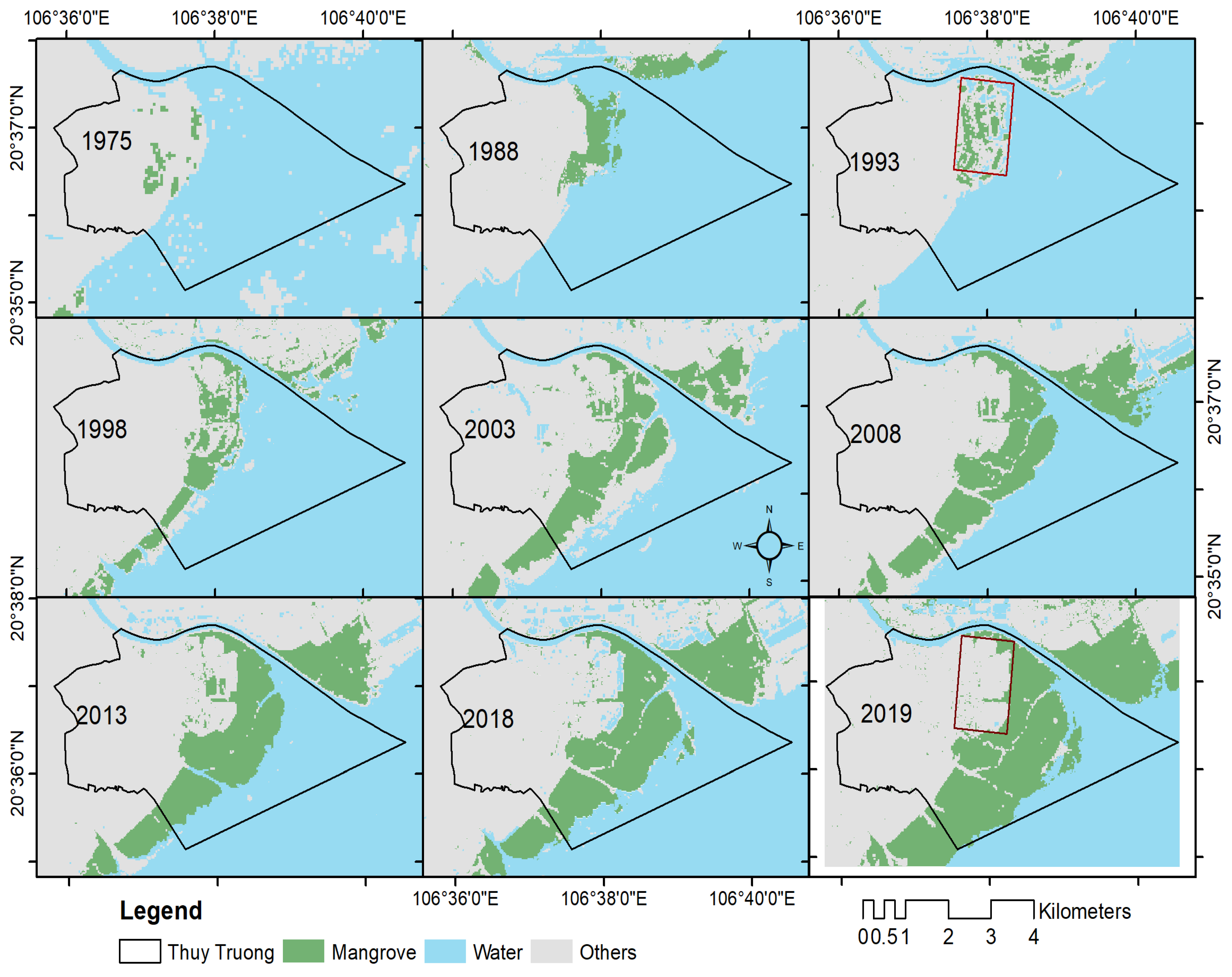
3.4. Mangrove Extent Changes

Extracting mangrove extents over a long period of time (1975–2019) showed the expansion, approximately 80 m/year, of the mangrove forest to about 3.5 km seaward in Thuy Truong commune and surroundings (Figure 7). The mangrove expansion of the results of the ISODATA classifications was slower between 1975 and 1993, and slightly decreased in 1993 compared to 1988. Nonetheless, the forest has been rapidly and continuously increasing in extent for 31 years from 1998 to 2019. Based on the in situ investigation data, the mangrove forest was mostly planted when the accumulated sediment from the river was high and the base well-founded. There is a small area of mangrove fragmentation due to aquaculture ponds and the mangrove there was degraded until 2019, by which time it had mostly disappeared (see the red rectangle in years 1993 and 2019). We also tested classifying the mangrove extents using the K-means classifier. However, no significant differences between the two methods were found. Hence, we only present the ISODATA results.
Changes in mangrove extent (including all mangrove species) in ha were quantified and graphed (Figure 8). In the first 11 years, the forest expanded approximately 150 ha (1988), but had decreased by slightly over 100 ha five years later (1993). Forest extent recovered slightly by 1998, and then increased by more than 220 ha in the five years until 2003. Afterward, there was a gradually increase over the subsequent 15 years (2003–2018). A remarkable increase was found in the last year of the assessment time. It is noted that all estimates were not validated except for 2019, for which ground-truth data were available. However, the mangrove in this region grows in sediment deposits and does not mix with other vegetation, therefore unsupervised classifications are considered sufficiently accurate.

3.5. Accuracy Assessment

3.5.1. Mangrove Age Classification

The producer and user, overall accuracy, and Kappa coefficient calculated from the four confusion matrices developed based on comparisons of the ground truth data and results of the four image classification methods (DT, ANN, FR, and SVM) for ten classes are summarized in Table 3. Although we calculated accuracy for all ten classes, we focused on three target layers of mangrove age (older than 10 years, around five years, and younger than three years). In general, the ten-year mangrove was classified at the highest accuracy (producer accuracy greater than 72.45% and user accuracy greater than 69.2%) and the five-year mangrove was the lowest (producer accuracy of 62.31% and user accuracy of 36.28%), with the exception of the low accuracy of the RF method for three-year mangroves (producer accuracy of 31.44% and user accuracy of 46.41%). With other layers, seawater was the most accurate classification, followed by river and mangrove, while road and residence were the least accurate. Comparing between the methods used (see the overall and the Kappa coefficients), the DT and SVM generated the most accurate results. RF revealed some limitations, particularly with highly mixed-pixel classes such as residence, road (narrow and long), and aquaculture.

3.5.2. Mangrove Species Classification

The support vector machine performances using Sentinel-1 and SPOT-7 fused images were evaluated by accuracy indexes and the Kappa coefficients (Table 4) for nine classes including mangrove species (Su, Vet, and Ban). Overall, all classes were categorized at high accuracy with around 90% overall accuracy. The Su mangrove (A. corniculatum) was the most accurate separation, followed by Vet (K. obovata) and Ban (S. caseolaris). Water-related layers like aquaculture, river, and seawater were the most accurate categories in contrast to bare land, which had the largest associated uncertainty. The Sentinel-1 VV polarization represented a better data source for mangrove type classification, regardless of image fusion technique, with an overall accuracy of 93% and Kappa coefficient of 0.92; compared to the use of Sentinel-1 VH polarization with overall accuracy of 89% and Kappa coefficient of 0.88. The PCA fusion method produced slightly better accuracy than the GS method, in most cases. It was interesting to look at the accuracy of the SPOT-7 and Sentinel-1 classifications with contradictory results, where the mangrove types were classified at low accuracy (around 50%) using the original SPOT-7 image, while the other classes were well separated (above 90%). UsingSentinel-1 provided the high accuracy of mangrove type and water (river and seawater) classifications (90%), in contrast, other classes such as agriculture and residence were mostly indistinguishable, with producer and user accuracies lower than 20%. This inconsistency of the producer and user accuracies of SPOT-7 and Sentinel-1 made the overall accuracies and the Kappa coefficients lower than those of the fused images for approximately 15% of SPOT-7 and 30% of Sentinel-1.

3.5.3. Mangrove Extent Classification

Two confusion matrices were calculated using the ground-truth region of interest for seven classes: mangrove, aquaculture, residence, agriculture, bare land, river, and seawater. The accuracy index of producer, user accuracy, and Kappa coefficients was summarized (Table 5). With only a small number of mangrove pixels misclassified to aquaculture (compared to total pixels), the errors were low, resulting in high user accuracy of mangrove class (97.29%). In general, agriculture and aquaculture, with highly mixed pixels, suffered low accuracy. It is noted that the main task of this classification was for the mangrove layer, however, other classes would have affected the mangrove classification result. Therefore, the road, which was a reported source of error, was left out in this task, after which, the overall accuracy improved. The table showed that the accuracy of the ISODATA was slightly higher than the K-means: approximately 5% of the overall accuracy and 0.06 of the Kappa coefficient. While the seawater presented the most accurate layer, the residence in the ISODATA results (88.11%) and the aquaculture of K-means (76.32%) were classified at the lowest accuracy.

4. Discussion

Scientists and researchers have attempted to improve the accuracy of remote sensing image classification for many uses including mangrove classifications [31,72]. Consequently, dozens of image classifiers have been developed and separated into supervised and unsupervised methods [6,73]. Each classifier has its own advantages and disadvantages for a particular use, therefore choosing a single “best” classification method is a challenge. In this study, we used four machine learning algorithms: ANN, DT, RF, and SVM for mangrove age and species classification. SVM demonstrated the greatest accuracy, however it would be premature to conclude that the SVM is better than the others in remotely sensed data classification and the results found here will need to be supported by further case studies.
Image fusion is considered to improve the quality of fused images [11,74] and allows the use of different sources of data for specific applications, particularly in the context of increasing remote sensing availability. Fusing optical and SAR remote scenes is commonly undertaken to enhance cartographic object extraction and improve spatial resolution [14] as well as reducing the effects of clouds in optical images [10,15,75]. It is nevertheless difficult to say whether fused images are always better for a particular use or not. Combining more data layers can be a source of error if the added information does not support the target aim. Therefore, image pre-processing implementation is sometimes needed alongside references to previous literature. For example, we undertook backscatter analyses (Figure 9) to develop a better understanding of SAR backscatter distributions under different LULC. This allowed us to decide which data were best used for what purpose. Figure 9A’s mean backscatter values for mangrove age (10, 5, and 3 years) were similar to the values for the agriculture, road, and bare land classes (both VH and VV polarizations), therefore justifying the use of Sentinel-1 data for the mangrove age classification. The mean backscatter values of mangrove species (Su, Vet, and Ban) were distinguished clearly from the mean values in other layers (Figure 9B), especially with the Sentinel-1 VV polarization. This could explain why the use of Sentinel-1 VV polarization generated the most accurate mangrove species classification.
Optical remote sensing, here using SPOT-7, was suitable for mangrove age and growth classification, but showed more limited capacity for classifying mangrove species for the study site of Thuy Truong. First, the received reflectance values from green vegetation surfaces (here mangrove) in optical images varied with wavelength (bands) [76]. With the SPOT-7 multispectral bands of Blue (0.455 µm–0.525 µm), Green (0.530 µm–0.590 µm), Red (0.625 µm–0.695 µm), and Near-Infrared (0.760 µm–0.890 µm), the mangrove could be discriminated from other land uses [77], even considering different ages and growth stages [78]. However, minor differences in reflectance between mangrove species could be found at the 0.760 µm–0.890 µm (NIR) [79]. In addition, the Ban mangrove (Figure 10A), Vet (Figure 10B), and Su (Figure 10C) were very similar in terms of stand, leaf, and stems based on our observations, so this also makes it difficult to discriminate between them.
In terms of LULC classification accuracy in remotely sensed data processes, confusion matrices are most frequently used [71] to provide analyses of the spatial distribution of errors and a better understanding of non-stationarity in land cover errors [80]. Although these measures of accuracy are very simple [81] and widely used, it is critical that the sources of errors are not revealed. Pontius and Millones (2011) identified limitations of the Kappa indices, for example, it does not report the correct proportion, and gives information that is redundant or misleading for practical decision making [82]. With identical inputs, and comparing the accuracy of results across two or more algorithms, we could determine which method tends to generate better outputs given our specific aim. However, it is still difficult to quantify method-based errors. Uncertainty could come from the data used, perhaps as a mixed-pixel problem related to coarse spatial resolution [83], geographical distortions, atmospheric effects, or seasonal effects [84]. To prevent the effects of seasonal changes on the mangrove surface from impacting on the image classification results, we tried to collect the Landsat-X images in the same season of autumn (October–November). However, this is sometimes a challenging task.
It is useful to look at the past to understand how the present situation was reached. Mangrove extent changes have been explored by many researchers [28,31,85] to inform management practices and protect habitats. Thanks to Earth observation data archives, the ability to use remotely sensed data in these assessments is becoming more widely available and often free of charge. Most studies investigate negative aspects such as mangrove degradation, fragmentation, and conversion to other land use types [32,86,87,88]. Our study has found a positive outcome, with mangrove forest developing from nearly nothing (in 1975) into a large mangrove forest (in 2019), thanks to efforts of the local community, government, and philanthropic projects. Ground-truth data cannot be obtained from the past to undertake supervised mangrove classification, but the unsupervised approaches, considered less accurate than supervised algorithms [6], remain helpful. The changes in mangrove extent in Thuy Truong identified in this study and the methods for using remotely sensed data tested will be valuable to monitoring and evaluation assessments of plantation projects in the region.

5. Conclusions

We report the use of four machine learning algorithms: ANN, DT, RF, and SVM for classifying mangrove ages. The estimated ages agreed well with the ground-truth field data, and the SVM was found to be the most accurate algorithm for mangrove species classification. Sentinel-1 backscatter mechanisms for different mangrove species are basically a function of tree structure, height, and density, which, combined with multispectral bands of SPOT-7, allowed us to discriminate between the Ban mangrove, Su, and Vet at an acceptable accuracy. Our assessment of multi-decadal mangrove changes in extent used the Landsat-X image series. We found a fluctuation in the first two decades, then a constant expansion of mangrove forest during the period 1998 to 2019. For the accuracy assessment, confusion matrices, producer–user accuracy, overall accuracy, and Kappa coefficients were used to measure the extent of agreement between image-based extraction and ground-truth data. These accuracy indices showed that all the classifications were accurate, and generally greater than 75%. Further research should test SAR and optical image fusion on other mangrove species as we found supportive information of SAR backscatters for classifying different mangrove species, and gained finer resolution of the panchromatic layer of optical images.

Author Contributions

Conceptualization, N.H.Q., C.R.H., L.C.S., and L.T.V.H.; Methodology, N.H.Q., L.C.S., R.C., and C.H.Q.; Field investigation, D.V.T., R.C., C.R.H., and N.H.Q.; Data analysis, N.H.Q., P.T.T.N., C.H.Q., D.V.T., and L.T.V.H.; Writing—original draft preparation, N.H.Q.; Writing—review and editing, N.H.Q., C.R.H., C.H.Q., L.C.S., P.T.T.N, L.T.V.H., R.C., and D.V.T; Visualization, N.H.Q., R.C., and C.R.H.; Supervision, C.H.Q., L.C.S., P.T.T.N., and L.T.V.H.; Project administration, C.H.Q. and L.T.V.H. All authors have read and agreed to the published version of the manuscript.

Funding

This research was financially supported by the Newton RCUK-SEAMED project “Harnessing multiple benefits from resilient mangrove systems” funded by NAFOSTED RCUK, ESRC reference: ES/R003300/1. Publication was supported by UKRI via the University of Leeds Open Access Fund.

Acknowledgments

The authors would like to thank all the anonymous reviewers and the assistant editor Ms. Milica Kovačević for their constructive comments and suggestions on this manuscript.

Conflicts of Interest

The authors declare no conflicts of interest.

Abbreviations

List of abbreviations in this study.
NoAbbreviationFull Name
1ANNArtificial Neural Network
2DTDecision Tree
3GPSGlobal Positioning System
4GSGram–Schmidt
5HHorizontal
6IHSIntensity-Hue-Saturation
7ISODATAIterative Self-organizing Data Analysis Technique
8LULCLand Use and Land Cover
9MSMultispectral
10NIRNear Infrared
11PANPanchromatic
12PCAPrincipal Component Analysis
13RFRandom Forest
14RRDRed River Delta
15SARSynthetic Aperture Radar
16SVMSupport Vector Machine
17USGSUnited States Geological Survey
18VVertical

References

  1. Cummings, C.A.; Todhunter, P.E.; Rundquist, B.C. Using the Hazus-MH flood model to evaluate community relocation as a flood mitigation response to terminal lake flooding: The case of Minnewaukan, North Dakota, USA. Appl. Geogr. 2012, 32, 889–895. [Google Scholar] [CrossRef]
  2. Heenkenda, M.K.; Joyce, K.E.; Maier, S.W.; de Bruin, S. Quantifying mangrove chlorophyll from high spatial resolution imagery. ISPRS J. Photogramm. Remote Sens. 2015, 108, 234–244. [Google Scholar] [CrossRef]
  3. VEA, The Vietnam environment administration. In Ministry of Natural Resources and Environment; 2016. Available online: http://vea.gov.vn/vn/truyenthong/biendoikhihau/Pages/90KH.aspx (accessed on 28 October 2019).
  4. Hoa, N.H. Using Landsat imagery and vegetation indices differencing to detect mangrove change: A case in Thai Thuy District, Thai Binh Province. J. For. Sci. Technol. 2016, 5, 59–66. [Google Scholar]
  5. Bakhtiyari, M.; Lee, S.Y.; Warnken, J. Seeing the forest as well as the trees: An expert opinion approach to identifying holistic condition indicators for mangrove ecosystems. Estuar. Coast. Shelf Sci. 2019, 222, 183–194. [Google Scholar] [CrossRef]
  6. Hasmadi, M.; Pakhriazad, H.; Shahrin, M. Evaluating supervised and unsupervised techniques for land cover mapping using remote sensing data. Geogr. Malays. J. Soc. Space 2009, 5, 1–10. [Google Scholar]
  7. Hepner, G.; Logan, T.; Ritter, N.; Bryant, N. Artificial neural network classification using a minimal training set- Comparison to conventional supervised classification. Photogramm. Eng. Rem. Sci. 1990, 56, 469–473. [Google Scholar]
  8. Sohn, Y.; Rebello, N.S. Supervised and unsupervised spectral angle classifiers. Photogramm. Eng. Rem. Sci. 2002, 68, 1271–1282. [Google Scholar]
  9. Amarsaikhan, D.; Douglas, T. Data fusion and multisource image classification. Int. J. Remote Sens. 2004, 25, 3529–3539. [Google Scholar] [CrossRef]
  10. Belgiu, M.; Stein, A. Spatiotemporal Image Fusion in Remote Sensing. Remote Sens. 2019, 11, 818. [Google Scholar] [CrossRef] [Green Version]
  11. Mangolini, M. Apport de la fusion d’images satellitaires multicapteurs au niveau pixel en télédétection et photo-interprétation. Ph.D. Thesis, Université de Nice Sophia-Antipolis, Nice, France, 1994. [Google Scholar]
  12. Ehlers, M. Spectral characteristics preserving image fusion based on Fourier domain filtering. in Remote Sensing for Environmental Monitoring, GIS Applications, and Geology IV. In Proceedings of the International Society for Optics and Photonics (SPIE), SPIE Bellingham, WA, USA, 22 October 2004. [Google Scholar]
  13. Rokni, K.; Ahmad, A.; Solaimani, K.; Hazini, S. A new approach for surface water change detection: Integration of pixel level image fusion and image classification techniques. Int. J. Appl. Earth Obs. 2015, 34, 226–234. [Google Scholar] [CrossRef]
  14. Pohl, C.; van Genderen, J.L. Review article multisensor image fusion in remote sensing: Concepts, methods and applications. Int. J. Remote Sens. 1998, 19, 823–854. [Google Scholar] [CrossRef] [Green Version]
  15. Quang, N.H.; Tuan, V.A.; Hao, N.T.P.; Hang, L.T.T.; Hung, N.M.; Anh, V.L.; Phuong, L.T.M.; Carrie, R. Synthetic aperture radar and optical remote sensing image fusion for flood monitoring in the Vietnam lower Mekong basin: A prototype application for the Vietnam Open Data Cube. Eur. J. Remote Sens. 2019, 52, 599–612. [Google Scholar]
  16. Solberg, A.H.S.; Jain, A.K.; Taxt, T. Multisource classification of remotely sensed data: Fusion of Landsat TM and SAR images. IEEE Trans. Geosci. Remote 1994, 32, 768–778. [Google Scholar] [CrossRef]
  17. Wang, L.; Jia, M.; Yin, D.; Tian, J. A review of remote sensing for mangrove forests: 1956–2018. Remote Sens. Environ. 2019, 231, 111223. [Google Scholar] [CrossRef]
  18. Pham, T.D.; Le, N.N.; Ha, N.T.; Nguyen, L.V.; Xia, J.; Yokoya, N.; To, T.T.; Trinh, H.X.; Kieu, L.Q.; Takeuchi, W. Estimating Mangrove Above-Ground Biomass Using Extreme Gradient Boosting Decision Trees Algorithm with Fused Sentinel-2 and ALOS-2 PALSAR-2 Data in Can Gio Biosphere Reserve, Vietnam. Remote Sens. 2020, 12, 777. [Google Scholar] [CrossRef] [Green Version]
  19. Proisy, C.; Couteron, P.; Fromard, F. Predicting and mapping mangrove biomass from canopy grain analysis using Fourier-based textural ordination of IKONOS images. Remote Sens. Environ. 2007, 109, 379–392. [Google Scholar] [CrossRef]
  20. Wicaksono, P.; Danoedoro, P.; Hartono; Nehren, U. Mangrove biomass carbon stock mapping of the Karimunjawa Islands using multispectral remote sensing. Int. J. Remote Sens. 2016, 37, 26–52. [Google Scholar] [CrossRef]
  21. Aslan, A.; Rahman, A.F.; Warren, M.W.; Robeson, S.M. Mapping spatial distribution and biomass of coastal wetland vegetation in Indonesian Papua by combining active and passive remotely sensed data. Remote Sens. Environ. 2016, 183, 65–81. [Google Scholar] [CrossRef]
  22. Vidhya, R.; Vijayasekaran, D.; Farook, M.A.; Jai, S.; Rohini, M.; Sinduja, A.; Vi, C.; Vi, W.G. Improved classification of mangroves health status using hyperspectral remote sensing data. Int. Arch. Photogramm. Remote Sens. Spat. Inf. Sci. 2014, 40, 667. [Google Scholar] [CrossRef] [Green Version]
  23. Chellamani, P.; Singh, C.P.; Panigrahy, S. Assessment of the health status of Indian mangrove ecosystems using multi temporal remote sensing data. Trop. Ecol. 2014, 55, 245–253. [Google Scholar]
  24. Hernández-Clemente, R.; North, P.R.; Hornero, A.; Zarco-Tejada, P.J. Assessing the effects of forest health on sun-induced chlorophyll fluorescence using the FluorFLIGHT 3-D radiative transfer model to account for forest structure. Remote Sens. Environ. 2017, 193, 165–179. [Google Scholar] [CrossRef] [Green Version]
  25. Mohammed, G.H.; Colombo, R.; Middleton, E.M.; Rascher, U.; van der Tol, C.; Nedbal, L.; Goulas, Y.; Pérez-Priego, O.; Damm, A.; Meroni, M.; et al. Remote sensing of solar-induced chlorophyll fluorescence (SIF) in vegetation: 50 years of progress. Remote Sens. Environ. 2019, 231, 111177. [Google Scholar] [CrossRef]
  26. Pastor-Guzman, J.; Atkinson, P.M.; Dash, J.; Rioja-Nieto, R. Spatiotemporal variation in mangrove chlorophyll concentration using Landsat 8. Remote Sens. 2015, 7, 14530–14558. [Google Scholar] [CrossRef] [Green Version]
  27. Vaiphasa, C. Remote sensing techniques for mangrove mapping. Ph.D. Thesis, International Institute for Geo-information Science and Earth Observation (ITC), Enschede and Wageningen University, Enschede, The Netherlands, 2006. [Google Scholar]
  28. Green, E.P.; Clark, C.D.; Mumby, P.J.; Edwards, A.J.; Ellis, A.C. Remote sensing techniques for mangrove mapping. Int. J. Remote Sens. 1998, 19, 935–956. [Google Scholar] [CrossRef]
  29. Blasco, F.; Gauquelin, T.; Rasolofoharinoro, M.; Denis, J.; Aizpuru, M.; Caldairou, V. Recent advances in mangrove studies using remote sensing data. Mar. Freshwater Res. 1998, 49, 287–296. [Google Scholar] [CrossRef] [Green Version]
  30. Hoan, N.T.; Duong, N.D.; Tateishi, R. Combination of ADEOS II–GLI and MODIS 250m Data for Land Cover Mapping of Indochina Peninsula. In Proceedings of the 26th Asian Conference on Remote Sensing and 2nd Asian Space Conference, Hanoi, Vietnam, 7–11 November 2005. [Google Scholar]
  31. Lymburner, L.; Bunting, P.; Lucas, R.; Scarth, P.; Alam, I.; Phillips, C.; Ticehurst, C.; Held, A. Mapping the multi-decadal mangrove dynamics of the Australian coastline. Remote Sens. Environ. 2020, 238, 111185. [Google Scholar] [CrossRef]
  32. Long, J.B.; Giri, C. Mapping the Philippines’ mangrove forests using Landsat imagery. Sensors 2011, 11, 2972–2981. [Google Scholar] [CrossRef] [Green Version]
  33. Tong, P.H.S.; Auda, Y.; Populus, J.; Aizpuru, M.; Habshi, A.A.; Blasco, F. Assessment from space of mangroves evolution in the Mekong Delta, in relation to extensive shrimp farming. Int. J. Remote Sens. 2004, 25, 4795–4812. [Google Scholar] [CrossRef]
  34. Tri, N.H.; Adger, W.; Kelly, P. Natural resource management in mitigating climate impacts: The example of mangrove restoration in Vietnam. Glob. Environ. Chang. 1998, 8, 49–61. [Google Scholar]
  35. Tri, N.H.; Adger, W.N.; Kelly, P.M. Social vulnerability to climate change and extremes in coastal Vietnam. World Dev. 1999, 27, 249–269. [Google Scholar]
  36. Pham, Q.T. An analysis of soil characteristics for agricultural land use orientation in Thai Thuy District, Thai Binh Province. VNU J. Sci. Earth Sci. 2007, 23, 105–109. [Google Scholar]
  37. Powell, N.; Osbeck, M.; Tan, S.B.; Toan, V.C. Mangrove restoration and rehabilitation for climate change adaptation in Vietnam. World Resources Report, Washington DC. World Resour. Rep. 2011, 1–22. [Google Scholar]
  38. Macintosh, D.J.; Ashton, E.C. A Review of Mangrove Biodiversity Conservation and Management; Centre for Tropical Ecosystems Research: Aarhus, Denmark, 2002. [Google Scholar]
  39. Giang, H.; Manh, D.; Huy, N. Use of Salt-Marsh Site Classification for Mangrove Forest Development and Reforestation in the Coastal Area of Thai Binh Province in the Context of Climate Change. In International Conference on Asian and Pacific Coasts; Springer: Berlin/Heidelberg, Germany, 2019. [Google Scholar]
  40. Ouaidrari, H.; Vermote, E.F. Operational atmospheric correction of Landsat TM data. Remote Sens. Environ. 1999, 70, 4–15. [Google Scholar] [CrossRef]
  41. Lu, D.; Mausel, P.; Brondizio, E.; Moran, E. Assessment of atmospheric correction methods for Landsat TM data applicable to Amazon basin LBA research. Int. J. Remote Sens. 2002, 23, 2651–2671. [Google Scholar] [CrossRef]
  42. Rahman, M.R.; Thakur, P.K. Detecting, mapping and analysing of flood water propagation using synthetic aperture radar (SAR) satellite data and GIS: A case study from the Kendrapara District of Orissa State of India. Egypt. J. Remote Sens. Space Sci. 2017, 21, S37–S41. [Google Scholar] [CrossRef]
  43. Cian, F.; Marconcini, M.; Ceccato, P. Normalized Difference Flood Index for rapid flood mapping: Taking advantage of EO big data. Remote Sens. Environ. 2018, 209, 712–730. [Google Scholar] [CrossRef]
  44. Nazim, K.; Ahmed, M.; Shaukat, S.S.; Khan, M.U.; Ali, Q.M. Age and growth rate estimation of grey mangrove Avicennia marina (Forsk). Vierh Pakistan. Pak. J. Bot. 2013, 45, 535–542. [Google Scholar]
  45. Duarte, C.M.; Thampanya, U.; Terrados, J.; Geertz-Hansen, O.; Fortes, M.D. The determination of the age and growth of SE Asian mangrove seedlings from internodal counts. Mangroves Salt Marshes. 1999, 3, 251–257. [Google Scholar] [CrossRef]
  46. Maxwell, A.E.; Warner, T.A.; Fang, F. Implementation of machine-learning classification in remote sensing: An applied review. Int. J. Remote Sens. 2018, 39, 2784–2817. [Google Scholar] [CrossRef] [Green Version]
  47. Yu, L.; Liang, L.; Wang, J.; Zhao, Y.; Cheng, Q.; Hu, L.; Liu, S.; Yu, L.; Wang, X.; Zhu, P.; et al. Meta-discoveries from a synthesis of satellite-based land-cover mapping research. Int. J. Remote Sens. 2014, 35, 4573–4588. [Google Scholar] [CrossRef]
  48. Foody, G.M. Relating the land-cover composition of mixed pixels to artificial neural network classification output. Photogramm. Eng. Rem. Sci. 1996, 62, 491–498. [Google Scholar]
  49. Dreiseitl, S.; Ohno-Machado, L. Logistic regression and artificial neural network classification models: A methodology review. J. Biomed. Inform. 2002, 35, 352–359. [Google Scholar] [CrossRef] [Green Version]
  50. Schalkoff, R. Pattern Recognition: Statistical, Structural and Neural Approaches; John Wiley: Toronto, ON, Canada, 1992. [Google Scholar]
  51. Pal, M.; Mather, P.M. An assessment of the effectiveness of decision tree methods for land cover classification. Remote Sens. Environ. 2003, 86, 554–565. [Google Scholar] [CrossRef]
  52. Brodley, C.E.; Utgoff, P.E. Multivariate Versus Univariate Decision Trees; Department of Computer and Information Science, University of Massachusetts: Amherst, MA, USA, 1992. [Google Scholar]
  53. Breiman, L. Random forests. Mach. Learn. 2001, 45, 5–32. [Google Scholar] [CrossRef] [Green Version]
  54. Noi, P.T.; Degener, J.; Kappas, M. Comparison of multiple linear regression, cubist regression, and random forest algorithms to estimate daily air surface temperature from dynamic combinations of MODIS LST data. Remote Sens. 2017, 9, 398. [Google Scholar] [CrossRef] [Green Version]
  55. Breiman, L. Bagging predictors. Mach. Learn. 1996, 24, 123–140. [Google Scholar] [CrossRef] [Green Version]
  56. Quinlan, J.R. C4. 5: Programs for Machine Learning; Elsevier: Amsterdam, The Netherlands, 2014. [Google Scholar]
  57. Ben-Hur, A.; Horn, D.; Siegelmann, H.T.; Vapnik, V. Support vector clustering. J. Mach. Learn. Res. 2001, 2, 125–137. [Google Scholar] [CrossRef]
  58. Vapnik, V.N. The Nature of Statistical Learning Theory; Springer: New York, NY, USA, 1995. [Google Scholar]
  59. Wu, T.F.; Lin, C.J.; Weng, R.C. Probability estimates for multi-class classification by pairwise coupling. J. Mach. Learn. Res. 2004, 5, 975–1005. [Google Scholar]
  60. Hsu, C.W.; Chang, C.C.; Lin, C.J. A Practical Guide to Support Vector Classification; National Taiwan University: Taipei, Taiwan, 2003; pp. 1396–1400. [Google Scholar]
  61. Laben, C.A.; Brower, B.V. Process for Enhancing the Spatial Resolution of Multispectral Imagery Using Pan-sharpening. U.S. Patent No. 6,011,875, 4 January 2000. [Google Scholar]
  62. Abdi, H.; Williams, L.J. Principal component analysis. Wiley Interdiscip. Rev. Comput. Stat. 2010, 4, 433–459. [Google Scholar] [CrossRef]
  63. Aiazzi, B.; Alparone, L.; Baronti, S.; Selva, M. MS+ Pan image fusion by an enhanced Gram–Schmidt spectral sharpening. In Proceedings of the 26th EARSeL symposium, Warsaw, Poland, 29 May–1 June 2006; Millpress: Rotterdam, The Netherlands, 2007. [Google Scholar]
  64. Kumar, U.; Mukhopadhyay, C.; Ramachandra, T. Pixel based fusion using IKONOS imagery. Int. J. Recent Trends Eng. 2009, 1, 173. [Google Scholar]
  65. Kamal, M.; Phinn, S. Hyperspectral data for mangrove species mapping: A comparison of pixel-based and object-based approach. Remote Sens. 2011, 3, 2222–2242. [Google Scholar] [CrossRef] [Green Version]
  66. Wang, L.; Sousa, W.P.; Gong, P.; Biging, G.S. Comparison of IKONOS and QuickBird images for mapping mangrove species on the Caribbean coast of Panama. Remote Sens. Environ. 2004, 91, 432–440. [Google Scholar] [CrossRef]
  67. Held, A.; Ticehurst, C.; Lymburner, L.; Williams, N. High resolution mapping of tropical mangrove ecosystems using hyperspectral and radar remote sensing. Int. J. Remote Sens. 2003, 24, 2739–2759. [Google Scholar] [CrossRef]
  68. Quang, N.H.; Tuan, V.A.; Le Hang, T.T.; Manh Hung, N.; Thi Dieu, D.; Duc Anh, N.; Hackney, C.R. Hydrological/Hydraulic Modeling-Based Thresholding of Multi SAR Remote Sensing Data for Flood Monitoring in Regions of the Vietnamese Lower Mekong River Basin. Water 2020, 12, 71. [Google Scholar] [CrossRef] [Green Version]
  69. El-Rahman, S.A. Hyperspectral image classification using unsupervised algorithms. IJACSA Int. J. Adv. Comput. Sci. Appl. 2016, 7, 198–205. [Google Scholar]
  70. Zhuang, X.; Engel, B.A.; Xiong, X.; Johannsen, C.J. Analysis of classification results of remotely sensed data and evaluation of classification algorithms. Photogramm. Eng. Remote Sci. 1995, 61, 427–432. [Google Scholar]
  71. Congalton, R.G. A review of assessing the accuracy of classifications of remotely sensed data. Remote Sens. Environ. 1991, 37, 35–46. [Google Scholar] [CrossRef]
  72. Kuenzer, C.; Bluemel, A.; Gebhardt, S.; Quoc, T.V.; Dech, S. Remote sensing of mangrove ecosystems: A review. Remote Sens. 2011, 3, 878–928. [Google Scholar] [CrossRef] [Green Version]
  73. Thakur, S.; Mondal, I.; Ghosh, P.B.; Das, P.; De, T.K. A review of the application of multispectral remote sensing in the study of mangrove ecosystems with special emphasis on image processing techniques. Spat. Inf. Res. 2020, 28, 39–51. [Google Scholar] [CrossRef]
  74. Ehlers, M. Multisensor image fusion techniques in remote sensing. ISPRS J Photogramm. 1991, 46, 19–30. [Google Scholar] [CrossRef] [Green Version]
  75. Lu, Z.; Dzurisin, D.; Jung, H.S.; Zhang, J.; Zhang, Y. Radar image and data fusion for natural hazards characterisation. Int. J. Image Data Fusion 2010, 1, 217–242. [Google Scholar] [CrossRef]
  76. Vaiphasa, C.; Ongsomwang, S.; Vaiphasa, T.; Skidmore, A.K. Tropical mangrove species discrimination using hyperspectral data: A laboratory study. Estuar. Coast. Shelf Sci. 2005, 65, 371–379. [Google Scholar] [CrossRef]
  77. Rahimizadeh, N.; Kafaky, S.B.; Sahebi, M.R.; Mataji, A. Forest structure parameter extraction using SPOT-7 satellite data by object-and pixel-based classification methods. Environ. Monit. Assess. 2020, 192, 43. [Google Scholar] [CrossRef] [PubMed]
  78. Rasolofoharinoro, M.; Blasco, F.; Bellan, M.F.; Aizpuru, M.; Gauquelin, T.; Denis, J. A remote sensing based methodology for mangrove studies in Madagascar. Int. J. Remote Sens. 1998, 19, 1873–1886. [Google Scholar] [CrossRef]
  79. Wan, L.; Lin, Y.; Zhang, H.; Wang, F.; Liu, M.; Lin, H. GF-5 Hyperspectral Data for Species Mapping of Mangrove in Mai Po, Hong Kong. Remote Sens. 2020, 12, 656. [Google Scholar] [CrossRef] [Green Version]
  80. Comber, A.; Fisher, P.; Brunsdon, C.; Khmag, A. Spatial analysis of remote sensing image classification accuracy. Remote Sens. Environ. 2012, 127, 237–246. [Google Scholar] [CrossRef] [Green Version]
  81. Story, M.; Congalton, R.G. Accuracy assessment: A user’s perspective. Photogramm. Eng. Remote Sci. 1986, 52, 397–399. [Google Scholar]
  82. Pontius, R.G.; Millones, M. Death to Kappa: Birth of quantity disagreement and allocation disagreement for accuracy assessment. Int. J. Remote Sens. 2011, 32, 4407–4429. [Google Scholar] [CrossRef]
  83. Hsieh, P.-F.; Lee, L.C.; Chen, N.-Y. Effect of spatial resolution on classification errors of pure and mixed pixels in remote sensing. IEEE Trans. Geosci. Remote 2001, 39, 2657–2663. [Google Scholar] [CrossRef]
  84. Hashiba, H.; Kameda, K.; Sugimura, T.; Takasaki, K. Analysis of landuse change in periphery of Tokyo during last twenty years using the same seasonal landsat data. Adv. Space Res. 1998, 22, 681–684. [Google Scholar] [CrossRef]
  85. Manson, F.; Loneragan, N.R.; McLeod, I.M.; Kenyon, R.A. Assessing techniques for estimating the extent of mangroves: Topographic maps, aerial photographs and Landsat TM images. Mar. Freshw. Res. 2001, 52, 787–792. [Google Scholar] [CrossRef]
  86. Vo, Q.T.; Oppelt, N.; Leinenkugel, P.; Kuenzer, C. Remote sensing in mapping mangrove ecosystems—An object-based approach. Remote Sens. 2013, 5, 183–201. [Google Scholar] [CrossRef] [Green Version]
  87. Kirui, K.B.; Kairo, J.G.; Bosire, J.; Viergever, K.M.; Rudra, S.; Huxham, M.; Briers, R.A. Mapping of mangrove forest land cover change along the Kenya coastline using Landsat imagery. Ocean Coast. Manag. 2013, 83, 19–24. [Google Scholar] [CrossRef]
  88. Terchunian, A.; Klemas, V.; Segovia, A.; Alvarez, A.; Vasconez, B.; Guerrero, L. Mangrove mapping in Ecuador: The impact of shrimp pond construction. Environ. Manag. 1986, 10, 345–350. [Google Scholar] [CrossRef]
Figure 1. Location of Thuy Truong commune (central coordinates of 106°38′00E and 20°36′00N) and in situ ground-truth investigation of mangrove locations. Plots for different types (yellow diamonds) and ages (blue diamonds) were positioned with confirmation of the local people. A GPS (Garmin Montana 680) with an integrated 5 M camera was used to locate and photograph each mangrove type and age. The SPOT-7 panchromatic band with the digital number ranged from 0 to 3946 was used for the base map.
Remotesensing 12 02289 g001
Figure 2. Flowchart of methodology used for mapping mangrove extent, age, and species. X refers to the mission number of the used Landsat images; ANN, DT, RF, SVM stand for artificial neural network, decision tree, random forest, and support vector machine, respectively; Mul and Pan are short forms of multispectral and panchromatic bands, respectively; GS and PCA indicate Gram–Schmidt and principal component analysis image fusion methods; V and H are vertical and horizontal, respectively, and coupled letters of VH and VV indicate Synthetic Aperture Radar (SAR) cross-polarizations.
Remotesensing 12 02289 g002
Figure 3. Classification of remote sensing data by an artificial neural network (adapted from Foody 1996) where Wij is the weight that connects the jth unit with its ith incoming connection; Oi and Oj are the value of the ith incoming connection and jth output connection; and λ is a gain parameter, which is often set to 1.
Remotesensing 12 02289 g003
Figure 4. Maps of classifications using the multispectral data of SPOT-7 acquired on 17 May 2019 for mangroves of ages older than 10 years, around five years, and younger than three years, mapped for the four classifiers of decision tree (A), artificial neural network (B), random forest (C), and support vector machine (D). The background is the SPOT-7 true-color composition image and the red polygon shows the border of the Thuy Truong commune.
Remotesensing 12 02289 g004
Figure 5. Demonstrations of SPOT-7 and Sentinel-1 (S1) image fusion processes where (A) is the original Sentinel-1 VH layer and (B) is Sentinel-1 VV layer (sigma0 in decibel); and (CF) depict the results of the fused images using VH–GS, VV–GS, VH–PCA, and VV–PCA, respectively.
Remotesensing 12 02289 g005
Figure 6. Maps of classified mangrove species; GS and PCA indicate Gram–Schmidt and principal component analysis image fusion methods; V and H are vertical and horizontal, respectively and coupled letters of VH and VV indicate SAR cross-polarizations. VH_GS, VH_PCA, VV_GS, and VV_PCA are combinations of fused images of SPOT-7 acquired on 17 May 2019 and Sentinel-1 polarization data (VH or VV) and the image fusion methods (GS or PCA).
Remotesensing 12 02289 g006
Figure 7. Changes in mangrove extent from 1975 to 2019 classified from a time series of Landsat images missions 2 to 8 (described in the Table 2) using the iterative self-organizing data analysis technique (ISODATA) classification, an unsupervised image classification approach (detailed in Section 2.3.1). The red rectangle denotes the same area of intensive aquaculture in 1993 and 2019.
Remotesensing 12 02289 g007
Figure 8. Total mangrove area (orange line) and changes in extent (blue line) (ha) from 1975–2019 in Thuy Truong commune.
Remotesensing 12 02289 g008
Figure 9. Sentinel-1 VH and VV backscatters on different land use and land cover; training data were used for (A) mangrove age and (B) mangrove species; V and H are vertical and horizontal, respectively, and coupled letters of VH and VV indicate SAR cross-polarizations.
Remotesensing 12 02289 g009
Figure 10. Pictures of three mangrove species taken by the authors in Thuy Truong commune on 22 November 2018.
Remotesensing 12 02289 g010
Table 1. In situ data for supervised remote sensing image classifications and accuracy evaluation. Examples of three existing mangrove species with scientific names, local names are marked in bold for illustration.
Training for Mangrove TypeNumber of PolygonsAverage Area (ha)Sum Area (ha)Training for Mangrove AgeNumber of PolygonsAverage Area (ha)Sum Area (ha)
Agriculture81.612.4Agriculture101.918.8
Aquaculture61.710.1Aquaculture122.226.3
Seawater421.586.1Seawater52.512.4
Bare land60.42.3Bare land140.23.2
Residence60.95.1Residence61.16.5
River73.927.4River81.814.4
Road70.10.6Road130.45.0
Sonneratia caseolaris (ban)92.118.9>10 year mangrove161.930.4
Aegiceras corniculatum (Su)91.311.35 year mangrove101.211.7
Kandelia obovata (Vet)160.57.4<3 year mangrove111.213.1
Sum78 (23) 181.6 105 (32) 141.6
Table 2. Summary of remote sensing data used (X refers to the Landsat mission of 2, 5, and 8; L1TP is data processing level 1 with precision terrain corrected; BQA stands for band quality; MSS is Multispectral Scanner Sensor; TM stands form; OLI is Operational Land Imager; Mul and Pan are short for multispectral and panchromatic bands, respectively; GPL is geometric processing level; RPL is radiometric processing level; and GRD is ground-range detected. V and H are vertical and horizontal, respectively, and coupled letters of VH and VV indicate SAR cross-polarizations).
DataTime of AcquisitionLevelBand and PolarizationResolution
Landsat (X)1975/04/20 (2MSS), 1988/11/04 (5TM), 1993/11/02 (5TM), 1998/10/15 (5TM), 2003/10/10 (5TM), 2008/11/11 (5TM), 2013/10/08 (8OLI), 2018/10/06 (8OLI), 2019/05/18 (8OLI)(2) L1TP, (5) L1TP, (5) L1TP, (5) L1TP, (5) L1TP, (5) L1TP, (8) L1TP, (8) L1TP, (8) L1TP,(2) 4–6, (5) 1–7, BQA, (5) 1–7, BQA, (5) 1–7, BQA, (5) 1–7, BQA, (5) 1–7, BQA, (8) 1–11, BQA, (8) 1–11, BQA, (8) 1–11, BQA.(2) 60 m (5) 30 m (5) 30 m (5) 30 m (5) 30 m (5) 30 m (8) 30 m, Pan (B8)15 m (8) 30 m, Pan (B8)15 m (8) 30 m, Pan (B8)15 m
SPOT-72019/05/17GPL: Sensor RPL: BasicBand 0–3 (Mul) Pan Mul 6 m Pan 1.5 m
Sentinel-12019/05/16 (ascending)L1 GRD productVH and VV10 m
Table 3. Accuracy indexes calculated from confusion matrices for mangrove age classification assessment. Prod. Acc. and User. Acc. are short forms of producer and user accuracy; DT, ANN, RF, and SVM indicate the image classification methods of decision tree, artificial neural network, random forest, and support vector machine, respectively.
ClassDTANNRFSVM
Prod. Acc. (Percent)User Acc. (Percent)Prod. Acc. (Percent)User Acc. (Percent)Prod. Acc. (Percent)User Acc. (Percent)Prod. Acc. (Percent)User Acc. (Percent)
Ten_Year_Mangrove93.8691.1493.3189.7772.4569.2094.6794.62
Five_Year_Mangrove72.3376.7459.5973.7062.3136.2884.3981.36
Three_Year_Mangrove79.1181.0170.3682.9231.4446.4191.0977.34
River97.4999.0593.8099.7997.5948.6298.5298.43
Aquaculture88.1786.4590.3278.4518.4960.0483.3894.37
Residence92.0991.8889.8470.2234.7018.9794.7093.39
Road89.3185.2890.4876.1719.2450.6877.6589.86
Agriculture98.7198.998.1497.8252.0378.0999.0099.59
Seawater10099.71100.0099.0399.3499.19100.00100.00
Bare land68.3180.21.8318.4846.4041.6284.1464.69
Overall Accuracy87%Overall Accuracy86.72%Overall Accuracy55.76%Overall Accuracy91.96%
Kappa Coefficient0.89Kappa Coefficient0.85Kappa Coefficient0.50Kappa Coefficient0.91
Table 4. Accuracy indexes calculated from confusion matrices for mangrove species classification assessment using SVM classifier, Prod. Acc. and User. Acc. are short forms of producer and user accuracy; VH_GS, VH_PCA, VV_GS, and VV_PCA are combinations of fused images of SPOT-7 and Sentinel-1 polarization data (VH or VV) and the image fusion methods (GS or PCA).
ClassVH_GSVH_PCAVV_GSVV_PCASPOT-7Sentinel-1
Prod. Acc. (Percent)User Acc. (Percent)Prod. Acc. (Percent)User Acc. (Percent)Prod. Acc. (Percent)User Acc. (Percent)Prod. Acc. (Percent)User Acc. (Percent)Prod. Acc. (Percent)User Acc. (Percent)Prod. Acc. (Percent)User Acc. (Percent)
Su (A. corniculatum)81.4681.9282.0382.7177.1492.9575.6393.3358.4371.6276.4493.23
Vet (K. obovata)87.3478.6588.1479.3994.1389.6094.4590.5051.2241.0393.8791.12
Ban (S. caseolaris)62.2575.8063.2476.2779.8454.5481.3151.4646.2550.1878.5662.63
Aquaculture90.9494.7191.0094.5498.9493.7298.9293.8695.3365.9545.2338.26
Agriculture99.2199.5099.2599.5299.88100.0099.88100.0098.6098.4818.9521.65
Residence97.5296.8997.2396.5396.5997.2996.5897.3196.0793.3318.4519.34
River99.8099.9899.8399.9897.2999.6397.2999.6397.4998.7389.3491.36
Bare land78.1161.4476.8861.3792.6564.9592.6168.3486.2586.2523.1531.21
Seawater80.3175.6383.2172.1497.6299.9797.6299.9799.9698.9794.1293.67
Overall Accuracy89%Overall Accuracy90%Overall Accuracy93%Overall Accuracy93%Overall Accuracy78%Overall Accuracy60%
Kappa Coefficient0.88Kappa Coefficient0.88Kappa Coefficient0.92Kappa Coefficient0.92Kappa Coefficient0.74Kappa Coefficient0.58
Table 5. Confusion matrices and accuracy indexes created for the unsupervised ISODATA and K-means classifiers using Landsat 8 acquired in 2019; Prod. Acc. and User. Acc. are short forms of producer and user accuracy; µ presents the averaged values.
ISODATA Classified (Pixels)Ground-Truth (Pixels)Summary
MangroveAquacultureResidenceAgricultureBare landRiverSeawaterTotalProd. Acc. (Percent)User Acc. (Percent)
Mangrove165025014241169699.1697.29
Aquaculture14905046711098397.0092.07
Residence00289040029388.1198.63
Agriculture020972110098593.8298.68
Bare land003945890063295.9393.20
River0000012439125298.8199.28
Seawater0100103382338499.7199.94
Total1664933328103661412583392922596.08µ97.01µ
Overall Accuracy = 97.89%Kappa Coefficient = 0.97
K-Means Classified (Pixels)Ground-Truth (Pixels)Summary
MangroveAquacultureResidenceAgricultureBare landRiverSeawaterTotalProd. Acc. (Percent)User Acc. (Percent)
Mangrove275466122810285289.7796.56
Aquaculture26166401026095276.3269.75
Residence00255090026495.8696.59
Agriculture100744370078295.3895.14
Bare land0010133940041787.9594.48
River52140000783097596.6780.31
Seawater00000028892889100100
Total30688702667804488102889913189.77µ96.56µ
Overall Accuracy = 92.90%Kappa Coefficient = 0.91

