Abstract
The first Chinese altimetry satellite, Haiyang-2A (HY-2A), which was launched in 2011, has provided a large amount of sea surface heights which can be used to derive marine gravity field. This paper derived the vertical deflections and gravity disturbances using HY-2A observations for the major area of the whole Earth’s ocean from 60°S and 60°N. The results showed that the standard deviations (STD) of vertical deflections differences were 1.1 s and 3.5 s for the north component and the east component between HY-2A’s observations and those from EGM2008 and EIGEN-6C4, respectively. This indicates the accuracy of the east component was poorer than that of the north component. In order to clearly demonstrate contribution of HY-2A’s observations to gravity disturbances, reference models and the commonly used remove-restore method were not adopted in this study. Therefore, the results can be seen as ‘pure’ signals from HY-2A. Assuming the values from EGM2008 were the true values, the accuracy of the gravity disturbances was about −1.1 mGal in terms of mean value of the errors and 8.0 mGal in terms of the STD. This shows systematic errors if only HY-2A observations were used. An index of STD showed that the accuracy of HY-2A was close to the theoretical accuracy according to the vertical deflection products. To verify whether the systematic errors of gravity field were from the long wavelengths, the long-wavelength parts of HY-2A’s gravity disturbance with wavelengths larger than 500 km were replaced by those from EGM2008. By comparing with ‘pure’ HY-2A version of gravity disturbance, the accuracy of the new version products was improved largely. The systematic errors no longer existed and the error STD was reduced to 6.1 mGal.
1. Introduction
Satellite altimetry plays a significant role in Earth science, such as marine gravity field recovery [1,2,3,4,5,6], ocean current inversion [7,8,9], seafloor topography estimation [10,11], geological interpretations [12,13,14,15], and so on. Due to its wide applications, since the first altimetry satellite experiments mission was developed by National Aeronautics and Space Administration (NASA) in 1973, several countries have launched altimetry satellites for various applications. As the first altimetry satellite developed by China, HY-2A (Haiyang-2A) was launched in 2011, and in 2016 its orbit was changed for conducting geodetic applications, i.e., marine gravity inversion.
Since HY-2A was launched, many scholars have discussed the accuracy of HY-2A altimetry sea surface height (SSH) observations and proposed methods to improve the accuracy. Bao et al. [16] presented the first accuracy assessment of HY-2A SSH and tested its mission requirements. Cui et al. [17] adopted Jason2 to reduce orbit errors of HY-2A by minimizing crossover differences between HY-2A and Jason2. Correspondingly, the standard deviation (STD) of self-crossover differences of HY-2A was decreased from 7.46 cm to 6.55 cm. Jiang et al. [18] reprocessed the SSH measurements from HY-2A radar altimeter and the STD of the crossover SSH differences for HY-2A was around 4.53 cm, which was largely improved when compared to that of HY-2A Interim Geophysical Data Record (IGDR) product. Zhang et al. [19] proved that HY-2A results were at a comparable level with respect to other missions like Jason-1 and CryoSat-2. These results indicate that HY-2A data can be used for Earth science research as other altimetry satellites.
Although for as nearly as four years, the orbit of HY-2A has been changed for geodetic mission, the performance of HY-2A in marine gravity derivation is not clear. Recently, an assessment of gravity anomaly accuracy derived from HY-2A was conducted in the South China Sea by Zhu et al. [20], in which the difference between HY-2A and ship-borne gravity was 5.91 mGal, showing that HY-2A can compete with other altimeter missions. Similar conclusions were also obtained by Zhang et al. [21], which pointed out that HY-2A is capable of improving marine gravity field modeling. In the studies of Zhu et al. [20] and Zhang et al. [21], full degrees of EGM2008 were selected as the reference model and the remove-restore method was used. Hence, the final gravity anomaly products also contained signals from EGM2008, which is a very accurate gravity field model. Although it is an effective way to use an accurate gravity field model to provide long-wavelength gravity signals and obtain highly accurate gravity field products, it is not clear how many contributions originate from HY-2A observations. In other words, if the remove-restore method is not used, what will the accuracy of the HY-2A gravity field be? In order to address this issue, the remove-restore method was not used in this study. The present study derived a gravity product between the latitudinal bounds of 60°S and 60°N. It needs to be noted that although the polar gravity data are also very important for Earth sciences, the polar regions are not considered in this study. The reason is that the inclination of HY-2A satellite is 99.34°, which leads to polar gaps with the spherical cap radius of 9.34°. Moreover, 60°S is not far from the Antarctica. For the Arctic Ocean, the accuracy of gravity derived in this area is not only influenced by the HY-2A observation accuracy, but also by values of the areas covered by ice, since the gravity inversion requires data over those areas. Due to these factors, the accuracy of the derived gravity in polar regions would be poorer than that in other ocean areas if the remove-restore method is not used. Instead, we derived gravity products for the major ocean area of the whole Earth from HY-2A. Furthermore, the vertical deflections, another set of important kind of gravity field products, were also derived in this paper.
Several methods can be used to derive marine gravity field using altimetry observations, such as the inverse Stokes formula [6,22], inverse Vening-Meinesz formula [1,2], least squares collocation method [20,23], etc. In this study, Sandwell’s method [3,4] was used, considering that it can be conducted easily by FFT (Fast Fourier Transform). Also, Sandwell’s method has no singular problems like those in the inverse Stokes and inverse Vening-Meinesz formulas, although some integral techniques have been proposed, such as those by Hwang et al. [1]. It needs to be pointed out that, if no remove-restore method is used, in which the long-wavelength part of gravity is replaced by the reference model [23], the results derived by Sandwell’s method are a different physical quantity in relation to those derived from the inverse Stokes and inverse Vening-Meinesz formulas. According to Heiskanen and Moritz [24], the physical quantity derived by Sandwell’s method is the gravity disturbance but not gravity anomaly, which is the derived quantity described by Hwang et al. [1] and Andersen et al. [6]. In order to distinguish these quantities, in this paper, we call it gravity disturbance but not gravity anomaly.
The main objective of this paper was to evaluate the global performance of the HY-2A geodetic mission by deriving vertical deflections and gravity disturbances using “pure” HY-2A altimetry observations. Accuracy assessments were then conducted on the derived products and strategies to improve the final gravity field products were also discussed. In Section 2, methods of vertical deflection computation and gravity disturbance inversion are presented. Section 3 shows data and editing criteria. Results and analysis are presented in Section 4. Discussion and conclusions are shown in Section 5 and Section 6, respectively.
2. Methods
2.1. Vertical Deflections Computation
Vertical deflections were computed at the crossover points as shown in Figure 1.
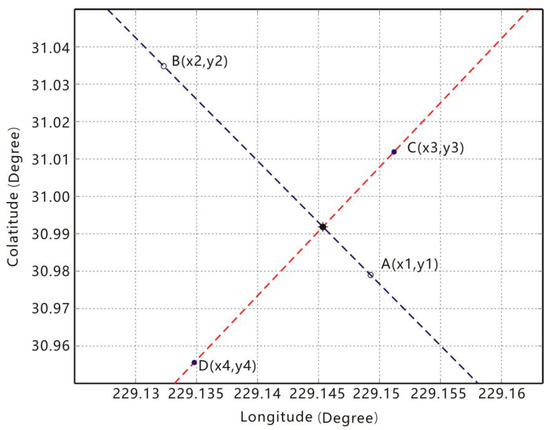
Figure 1.
Crossover point for computing vertical deflections.
In Figure 1, the blue and red lines represent the ascending and descending passes, respectively, and A, B, C, and D denote the four observation points near the crossover point. In order to derive vertical deflections, the derivative of the geoid height , with respect to time , along the orbit was first computed as [3]:
where and are the latitude and longitude, respectively, and subscripts and mean the values at the ascending and descending passes, respectively. From Equation (1), we can obtain:
Finally, vertical deflections can be obtained by Equation (3):
where is mean radius of the Earth.
2.2. Gravity Disturbance Computation
As long as vertical deflections are obtained, gravity disturbance, denoted as , can be derived from the formula given by Sandwell and Smith [3]:
where
means inverse FFT; is the mean value of gravity; and and are wavelengths of vertical deflections in and axes.
3. Data and Editing Criteria
Six cycles of HY-2A IGDR from National Satellite Ocean Administration Service of China (ftp2.nsoas.org.cn) were used. The time period was from March 30, 2016 to December 27, 2018. Using these data, SSH can be obtained by Equations (6) and (7) as:
where
is height of the HY-2A satellite above the reference ellipsoid; means the residual range observations, which is the range from the satellite to the sea surface; , , respectively, represent wet and dry troposphere corrections; means ionosphere correction; is sea state bias correction; , , are the solid, ocean, and pole tide corrections, respectively; and is inverse barometer correction. In the observations, many outlying values exist, which must be removed. Values exceeding the range given by Table 1 were removed. In this study, the geoid gradients were represented by gradients of SSH. This is because slope of the ocean surface caused by mean dynamic topography (MDT) is about 50-times smaller than the geoid slope [25,26]. Moreover, the influences of MDT can be weakened during the gradients’ computation [20].

Table 1.
Editing criteria of the HY-2A altimeter products.
Besides HY-2A observations, EGM2008 [27] and EIGEN6C [28] were selected as the checking models to evaluate accuracy of the gravity field products derived by HY-2A observations. These two models have a spatial resolution of about 10 km and high accuracy.
4. Results and Analysis
4.1. Vertical Deflections
In order to quantify the differences, the vertical deflections derived from HY-2A data (see Figure 2) and their equivalents from EGM2008 and EIGEN-6C4 were compared. It is worth noting that this comparison applied all the degrees and orders of the two gravity field models. However, in order to reduce computation time, when plotting Figure 3, only the former 360 degrees and orders of EGM2008 were used. Figure 3 was mainly used to demonstrate the spatial distribution of the differences. Three regions located in the Atlantic, Indian and Pacific oceans were selected as examples, and the statistics of their differences are given in Table 2. To affirm the results in Table 2, Figure 4 shows the summary statistics of vertical deflections obtained in these selected oceanic regions.
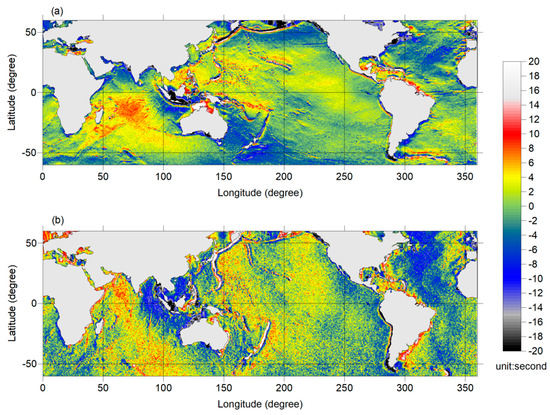
Figure 2.
Vertical deflections derived from HY-2A observations: (a) North component; (b) East component.
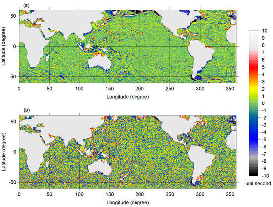
Figure 3.
Differences between vertical deflections derived from HY-2A observations and EGM2008: (a) North component; (b) East component.
Table 2.
Statistics of differences between vertical deflections from the HY-2A and gravity field models.
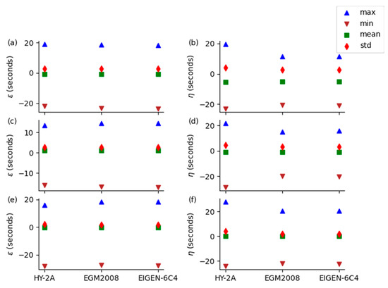
Figure 4.
Summary statistics of vertical deflections observed from HY-2A, EGM2008, and EIGEN-6C4 in the three selected oceanic regions: (a) North components in Atlantic Ocean; (b) East components in Atlantic Ocean; (c) North components in Indian Ocean; (d) East components in Indian Ocean; (e) North components in Pacific Ocean; and (f) East components in Pacific Ocean.
According to Figure 3, HY-2A products were consistent with those from EGM2008 and the differences of east component of vertical deflections were obviously larger than those of the north component. This point is also substantiated by the statistics in Table 2. Definitely, in these regions, STD of the differences between east component of vertical deflections derived from HY-2A and EGM2008 or EIGEN-6C4 were about three-times larger than those of the north component. This was not caused by contributions of winds and currents, because coherent current-related features were not present in the east component errors (see Figure 3b). Instead, it was mainly due to the fact that the vertical deflections were computed along the orbit in order to reduce systematic errors. However, the inclination of HY-2A orbit was close to 90° and was thus close to the direction from the south to north. Under the case of high inclination, the larger errors in east component of vertical deflections can be proven, in theory, by the covariance information of estimates of Equation (2) (see [3]) or the error propagation rule based on Equation (2). The phenomenon is common in altimetry products [3,29], because the inclinations of altimetry satellites are often designed to be close to 90° in order to obtain a larger observation coverage.
According to Table 2, STD of the differences were around 1.1 s and 3.5 s for the north component and east component, respectively. It should be noted that these comparisons were all conducted at crossover points, not the mean values of the grids. Hence, this performance index represents the initial vertical deflection accuracy of HY-2A observations. And then the accuracy of gravity anomalies, denoted as , can be evaluated by the relationship given by Molodensky [30,31]:
where is normal gravity; and , and denote STD of , , errors, respectively. Thus, if values of EGM2008 or EIGEN-6C4 are seen as the true values, the final gravity accuracy should be around 17.3 mGal and the contribution from the north component and east component should be about 4.7 mGal and 16.3 mGal, respectively. According to these values, it seems that the accuracy of the gravity would be poor, especially when compared with the results of Zhu et al. [20]. Indeed, this accuracy corresponds to one cycle’s observations since no grid processing was conducted. However, using observations from multiple cycles, random errors of the vertical deflections can be largely reduced, and the accuracy of gravity can be improved correspondingly. In this paper, six cycles’ observations were used. Thus, the STD of the gravity errors can be reduced by a factor , which corresponds to 7.1 mGal.
It is evident from Figure 4 that vertical deflections from HY-2A are comparable to those obtained from EGM2008 and EIGEN-6C4. However, the east-west components are slightly poorer. Figure 4 is a further substantiation of results in Table 2. In addition, the distributions of vertical deflections showed obvious geological features, such as the Western Pacific Ocean trench, where large values of vertical deflections existed. Definitely, the geological structure influences the distribution of vertical deflections. Conversely, it is possible to use the derived vertical deflections to inverse some geological structure, such as the bathymetry information, which should be studied in future.
4.2. Gravity Disturbance
With the six cycles of HY-2A observations, 30′ × 30′ vertical deflection grids were obtained. In each grid, mean value and STD of the HY-2A vertical deflections were first computed. Values that deviated from the mean by a margin greater than three-times the STD were removed. Finally, new grids of vertical deflections were obtained. In order to conduct the computations in Equation (4), data over land were also needed. However, HY-2A cannot provide vertical deflections over land area. Instead, values from former 360 degrees and orders of EGM2008 were used. In addition, the data in the ocean area where the water depths shallower than −1000 m were also provided by EGM2008. It needs to be noted that, in waters deeper than −1000 m, only HY-2A observations were used. The final gravity accuracy assessments were also only conducted over the areas where only HY-2A data was used.
The obtained gravity disturbance, , in the ocean area deeper than −1000 m, is given in Figure 5a. The differences between from HY-2A and those from 360 degrees and orders of EGM2008 are given in Figure 5b. The mean and STD of the differences were −1.1 mGal and 8.0 mGal in the whole region, respectively. In these statistics, values exceeding the mean errors by three-times the STD were removed, corresponding to about 3% of the data being removed. The value of 8.0 mGal was close to the theoretical accuracy of 7.1 mGal, which is described in previous section. The differences could mainly be attributed to computational errors and the long-wavelength part of the gravity signals.
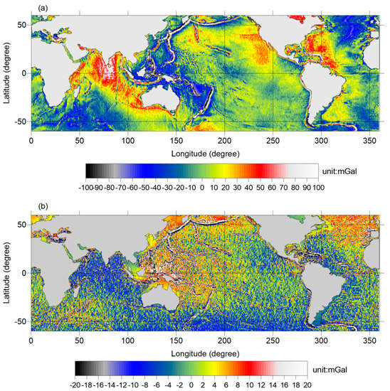
Figure 5.
derived from HY-2A (a) and the difference (b) between and those from EGM08.
According to Figure 5a, derived from HY-2A clearly demonstrated main signals of the Earth, such as the trench in the western Pacific. The differences between from HY-2A and EGM2008 were smaller than 10 mGal in major part of the study area. Large differences existed in the area near the island, such as the Philippine archipelago. This is consistent with the conclusions of Zhu et al. [20]. In addition, in the west Pacific and northeast Atlantic Ocean areas, the differences were slightly larger than other areas.
In order to further analyze the magnitude of the errors, statistics were conducted in terms of magnitudes of the errors, and the results are given in Table 3. According to the results, 57% of the errors were smaller than 6 mGal and 79% of the errors were smaller than 10 mGal. These results can be rather seen as ‘pure’ HY-2A signals compared to those of Zhu et al. [20] and Zhang et al. [21], since no reference models were used in the ocean area.
Table 3.
Error magnitude statistics.
The relationship between the inversion accuracy and the water depth was also investigated. Figure 6 shows the relationship between accuracy of the derived gravity disturbance and ocean water depth with an interval of −500 m. Obviously, the accuracy changed with varying water depths. For example, the error STD was smaller than 8 mGal if the water depths were deeper than −2000 m but shallower than −5500 m. In general, the error STD initially decreased and then increased. The accuracy was higher in the depths ranging from −4000–−5000 m compared to gravity disturbances in other depths. According to the error mean values, systematic errors existed. The mean values of the errors represent the magnitude of this kind of error, i.e., about 1.2 mGal. This means that only using HY-2A would make it difficult to derive the full wavelength of gravity signals.
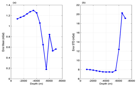
Figure 6.
Accuracy at different depth of the water: (a) Error mean values; (b) error STD values.
5. Discussion
5.1. Reduction of Systematic Errors
The fourth section analyzed the accuracy of ‘pure’ HY-2A gravity disturbance in oceans and found that systematic errors existed. To verify if this kind of error was from the long-wavelength gravity, a high-pass Gaussian filter with a band pass of 500 km was implemented on the grid values of derived from HY-2A. Signals with wavelengths longer than 500 km were replaced by those from EGM2008. In this study, 500 km corresponds to 40 degrees of the gravity field model, which is not high when compared to the reference models used in other studies. In other studies, such as Zhu et al. [20] and Zhang et al. [21], 2160 degrees of the gravity field models were usually used. We selected 500 km as the cutoff wavelength so as to reduce the influence of reference models. Finally, the combined was given in Figure 7b.
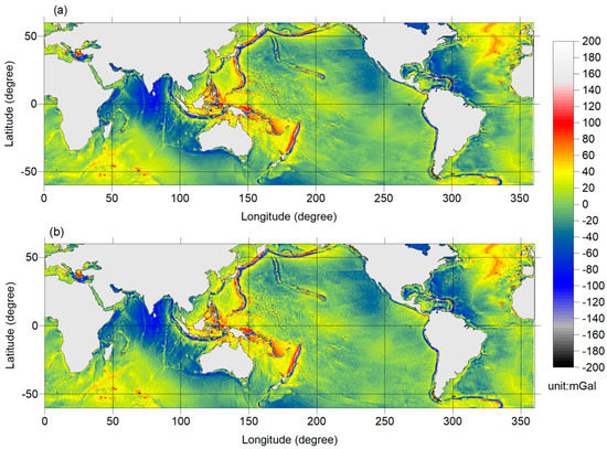
Figure 7.
Signals: (a) from EGM2008; (b) the combined .
With values from EGM2008 regarded as true values (shown in Figure 7a), the accuracy of the combined was evaluated, and the difference between it and EGM2008 was given in Figure 8. According to Figure 7, the two gravity maps show almost same signals, such as the strong signals in the Mariana Trench and negative values in the Northern Indian ocean, which reflect the mass distribution in the related area. Indeed, there were minor differences between the combined and EGM2008 values. In the whole study area, the mean and STD of the combined errors were −0.02 mGal and 6.1 mGal, respectively, which were definitely reduced compared to the initial and also ‘pure’ derived from HY-2A. Figure 9 gives the cumulative ratios of the errors in terms of magnitudes. According to this figure, 70% of the errors were smaller than 6 mGal, and 90% of the errors were smaller than 10 mGal. Compared with Table 3, this index was largely improved. Figure 10 gives the relationship between the accuracy of the new version of and the ocean depths. It proves again the improvement of the accuracy compared to that of the ‘pure’ HY-2A version.
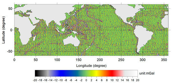
Figure 8.
The differences between from HY-2A (the combined version) and that from EGM2008.

Figure 9.
Ratio of the gravity disturbance error compared to EGM2008.
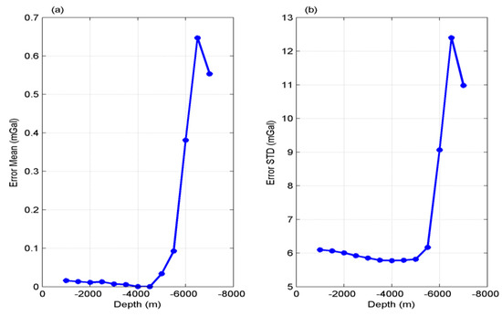
Figure 10.
Accuracy of the new version of with varying water depth: (a) Error mean values; (b) error STD values.
However, there were still large errors in deep oceanic regions. For example, in areas deeper than −6000 m, the error STD was larger than 9 mGal and even exceeded 12.4 mGal, which was twice as large as the STD of the whole area, i.e., 6.1 mGal. This means that other strategies should be adopted to improve the accuracy in such areas. The method provided by Sandwell and Smith [26] may be helpful in this regard, and should be studied further. Indeed, the deep ocean areas occupy only a small ratio of the whole study area. Figure 11 shows the number of the grids with water depths deeper than that given by X-axis. Definitely, the number of the grids with depths deeper than −6000 m was only around 1600, whereas there were more than 100,000 grids in the whole study area. Thus, areas deeper than −6000 m occupied no more than 0.15%.
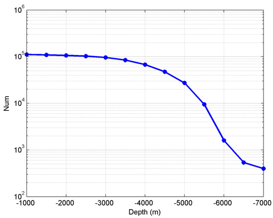
Figure 11.
Number of grids with different depths.
5.2. Inversion of Gravity Anomalies
There are at least two methods that can be used to derive gravity anomalies based on the results derived from Equation (4). The first method is the remove-store method. If a highly accurate gravity field model is used, such as 2160 degrees and orders of EGM2008, the results derived from Equation (4) can be seen as residual gravity anomalies [23]. These values are added to the gravity anomalies provided by the reference model, and new gravity anomalies are obtained. The second method uses the following formula to compute the gravity anomaly [6,23]:
where denotes gravity anomaly and , is geoid height. In this paper, in order to better demonstrate the performance of HY-2A, we adopted this latter method to derive the gravity anomaly. However, geoid heights cannot be provided by HY-2A directly. Instead, SSHs provided by HY-2A were used. In order to show the difference between and , a new variable was defined as
The distribution of is shown in Figure 12.
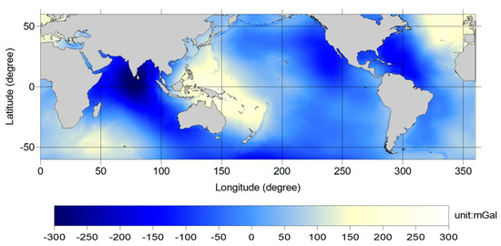
Figure 12.
Distribution of .
Then, was removed from , with the result shown in Figure 5a. Definitely, systematic errors also existed, as in the gravity disturbance. Hence, the long-wavelength part of the gravity anomaly must be replaced. Similar to Section 5.1, we used EGM2008 to provide a gravity anomaly with a wavelength larger than 500 km, and a new version of the gravity anomalies was obtained. The differences between the derived gravity anomalies and those from EGM2008 are shown in Figure 13. In the whole study area, the mean and STD of the differences were −0.005 mGal and 6.1 mGal, respectively, which are almost same as the results of the gravity disturbance.
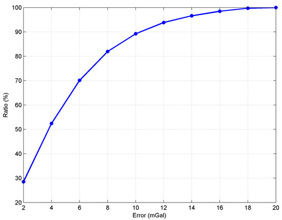
Figure 13.
Ratio of gravity anomaly errors compared to EGM2008.
The V29.1 version of gravity anomalies from Scripps Institution of Oceanography (SIO) was selected as another example for comparison. Similarly, in order to reduce the influence from the long-wavelength part, the part with wavelength longer than 500 km was replaced with that from SIO. Figure 14a shows the distribution of HY-2A derived gravity anomalies and Figure 14b shows the difference between gravity anomalies derived from HY-2A and V29.1. Assuming that V29.1 are the true values, Figure 15 shows the relationship between the errors and the depths. Table 4 gives statistics of the error magnitude for the entire study area.
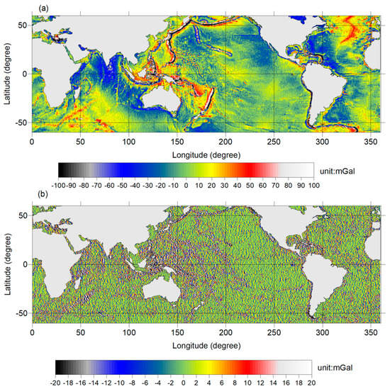
Figure 14.
(a) HY-2A-derived gravity anomaly and (b) differences between the HY-2A-derived gravity anomaly and SIO.
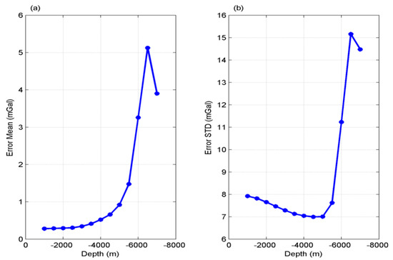
Figure 15.
Error compared to SIO gravity anomalies: (a) Absolute values of mean error; (b) error STD.
Table 4.
Statistics about the magnitude of gravity anomaly errors.
Obviously, the HY-2A-derived gravity anomalies had larger differences when compared with the SIO gravity anomalies than compared with EGM2008. The main reason was that vertical deflections over the land were provided by EGM2008. This means the values over land also contributed to marine gravity field inversion. However, the main signals were still from the observations in the ocean. According to Table 4, in 62% of the grids, the differences were smaller than 6 mGal. In the whole study area, i.e., areas with water deeper than −1000 m, the mean and STD of the differences were, respectively, −0.3 mGal and 7.9 mGal. According to these results, gravity anomalies with an accuracy higher than 8 mGal can be derived using HY-2A in major oceans of the Earth with no extra-high resolution of gravity field model used as a reference model.
It needs to be noted that the main objective of this study is to evaluate the global performance of HY-2A. Thus, this study tried to use as few signals from reference model as possible. If this point is not considered, several strategies can be used to improve the accuracy of HY-2A-derived gravity anomalies. These may include the remove-restore method, using a reference model with high resolution and accuracy for the whole area but not only providing values in the land area, and corrections for the area above ocean trenches and large seamounts [26]. Other techniques include using an MDT model to reduce the influences caused by the difference between SSH and geoid in Equation (9) [6,32]. Hence, it is possible to derive higher accurate marine gravity field using HY-2A observations, which should be studied further in the future. In addition, the derived gravity anomaly (see Figure 14a) shows abundant information on geological structure, such as oceanic trench, which also should be studied further [33], and should be combined with other gravity products from gravity satellites [34,35,36].
6. Conclusions
Vertical deflections and gravity disturbances were derived using six cycles of HY-2A observations. Compared with EGM2008 and EIGEN-6C4, the east component of HY-2A vertical deflections had a poorer accuracy than that of the north component nearly by three times. If only HY-2A observations were used, gravity disturbances had systematic errors with a magnitude of about 1 mGal. Also, 70% of the errors were smaller than 8 mGal, and 79% of the errors were smaller than 10 mGal in the study area. The systematic errors were mainly caused by the long-wavelength part of the gravity. This point was proved by the replacement of long-wavelength part of gravity by EGM2008, and the combined gravity disturbances were obtained. Correspondingly, compared to EGM2008, the accuracy was improved largely with no large systematic errors, and STD of the errors was reduced to 6 mGal. This means that by combining other sources of gravity data, especially accurate long-wavelength gravity such as gravity products from gravity satellites, an accurate marine gravity field can be obtained as other altimetry satellites.
Author Contributions
Conceptualization, X.W.; data curation, X.W. and R.F.A.; funding acquisition, X.W.; investigation, X.W., R.F.A. and X.G.; methodology, X.W. and S.J.; supervision, S.J.; writing—original draft, X.W; writing—review & editing, R.F.A., S.J., and X.G. All authors have read and agreed to the published version of the manuscript.
Funding
This research was funded by the National Natural Science Foundation of China (No. 41674026); National Key Research and Development Program of China Project (Grant No. 2018YFC0603502); Fundamental Research Funds for the Central Universities (No. 2652018027); Open Research Fund of Key Laboratory of Space Utilization, Chinese Academy of Sciences (LSU-KFJJ-201902); China Geological Survey (No.20191006); Qian Xuesen Lab.—DFH Sat. Co. Joint Research and Development Fund under grants (M-2017-006).
Acknowledgments
We thank all the reviewers for the comments which helped to greatly improve the manuscript. We also would like to thank National Satellite Ocean Application Service of China for providing HY-2A data.
Conflicts of Interest
The authors declare no conflict of interest.
References
- Hwang, C. Inverse Vening Meinesz formula and deflection-geoid formula: Applications to the predictions of gravity and geoid over the South China Sea. J. Geod. 1998, 72, 304–312. [Google Scholar] [CrossRef]
- Hwang, C.; Hsu, H.Y.; Jang, R.J. Global mean sea surface and marine gravity anomaly from multi-satellite altimetry: Applications of deflection-geoid and inverse Vening Meinesz formulae. J. Geod. 2002, 76, 407–418. [Google Scholar] [CrossRef]
- Sandwell, D.; Smith, W. Marine gravity anomaly from Geosat and ERS1 satellite altimetry. J. Geophys. Res. 1997, 102, 10039–10054. [Google Scholar] [CrossRef]
- Sandwell, D.; Smith, W. Global marine gravity from retracked Geosat and ERS-1 altimetry: Ridge segmentation versus spreading rate. J. Geophys. Res. 2009, 114, B01411. [Google Scholar] [CrossRef]
- Andersen, O.B.; Knudsen, P. Global marine gravity field from the ERS-1 and Geosat geodetic mission altimetry. J. Geophys. Res. 1998, 103, 8129–8137. [Google Scholar] [CrossRef]
- Andersen, O.; Knudsen, P.; Berry, P. The DNSC08GRA global marine gravity field from double retracked satellite altimetry. J. Geod. 2010, 84. [Google Scholar] [CrossRef]
- Bingham, R.J.; Knudsen, P.; Pail, P. An initial estimate of the North Atlantic steady-state geostrophic circulation from GOCE. Geophys. Res. Lett. 2011, 38. [Google Scholar] [CrossRef]
- Hwang, C.; Kao, R. TOPEX/POSEIDON-derived space–time variations of the Kuroshio Current: Applications of a gravimetric geoid and wavelet analysis. Geophys. J. Int. 2002, 151, 835–847. [Google Scholar] [CrossRef]
- Wan, X.; Yu, J. Mean dynamic topography calculated by GOCE gravity field model and CNES-CLS2010 mean sea surface height. Chin. J. Geophys. 2013, 56, 1850–1856. [Google Scholar] [CrossRef]
- Sandwell, D.T.; Müller, R.D.; Smith, W.H.F.; Garcia, E.; Francis, R. New global marine gravity model from CryoSat-2 and Jason-1 reveals buried tectonic structure. Science 2014, 346, 65–67. [Google Scholar] [CrossRef]
- Tozer, B.; Sandwell, D.T.; Smith, W.H.F.; Olson, C.; Beale, J.R.; Wessel, P. Global bathymetry and topography at 15 arc sec: SRTM15+. Earth Space Sci. 2019, 6. [Google Scholar] [CrossRef]
- Sazhina, N.; Grushinsky, N. Gravity Prospecting; University Press of the Pacific: Honolulu, HI, USA, 2004. [Google Scholar]
- Gaina, C.; Torsvik, T.H.; van Hinsbergen, D.J.J.; Medvedev, S.; Werner, S.C.; Labails, C. The African Plate: A history of oceanic crust accretion and subduction since the Jurassic. Tectonophysics 2013, 604, 4–25. [Google Scholar] [CrossRef]
- Yang, J.Y.; Zhang, X.H.; Zhang, F.F.; Hang, B.B.; Tian, Z.X. Preparation of the free-air gravity anomaly map in the seas of China and adjacent areas using multi-source gravity data and interpretation of the gravity field. Chin. J. Geophys. 2014, 57, 872–884. [Google Scholar]
- Eppelbaum, L.V.; Katz, Y.I. Significant tectono-geophysical features of the African-Arabian tectonic region: An overview. Geotectonics 2020, 54, 266–283. [Google Scholar] [CrossRef]
- Bao, L.; Gao, P.; Peng, H.; Jia, Y.; Shum, C.K.; Lin, M.; Guo, Q. First accuracy assessment of the HY-2A altimeter sea surface height observations: Cross-calibration results. Adv. Space Res. 2015, 55, 90–105. [Google Scholar] [CrossRef]
- Cui, W.; Wang, W.; Jie, Z.; Yang, J.; Jia, Y. Improvement of sea surface height measurements of HY-2A satellite altimeter using Jason-2. Mar. Geod. 2018. [Google Scholar] [CrossRef]
- Jiang, M.; Xu, K.; Liu, Y.; Zhao, J.; Wang, L. Assessment of reprocessed sea surface height measurements derived from HY-2A radar altimeter and its application to the observation of 2015–2016 El Niño. Acta Oceanol. Sin. 2018, 37, 115–129. [Google Scholar] [CrossRef]
- Zhang, S.; Li, J.; Jin, T.; Che, D. HY-2A Altimeter Data Initial Assessment and Corresponding Two-Pass Waveform Retracker. Remote Sens. 2018, 10, 507. [Google Scholar] [CrossRef]
- Zhu, C.; Guo, J.; Hwang, C.; Gao, J.; Yuan, J.; Liu, X. How HY-2A/GM altimeter performs in marine gravity derivation: Assessment in the South China Sea. Geophys. J. Int. 2019, 219, 1056–1064. [Google Scholar] [CrossRef]
- Zhang, S.; Andersen, O.B.; Kong, X.; Li, H. Inversion and Validation of Improved Marine Gravity Field Recovery in South China Sea by Incorporating HY-2A Altimeter Waveform Data. Remote Sens. 2020, 12, 802. [Google Scholar] [CrossRef]
- Olgiati, A.; Balmino, G.; Sarrailh, M.; Green, C.M. Gravity anomalies from satellite altimetry: Comparison between computation via geoid heights and via deflections of the vertical. Bull. Géodésique. 1995, 69, 252–260. [Google Scholar] [CrossRef]
- Hwang, C.; Parsons, B. An optimal procedure for deriving marine gravity from multi-satellite altimetry. Geophys. J. Int. 1996, 125, 705–718. [Google Scholar] [CrossRef]
- Heiskanen, W.A.; Moritz, H. Physical Geodesy; W.H. Freeman: New York, NY, USA, 1967. [Google Scholar]
- Stewart, R.H. Methods of Satellite Oceanography; University of California Press: San Diego, CA, USA, 1985; p. 360. [Google Scholar]
- Sandwell, D.; Smith, W. Slope correction for ocean radar altimetry. J. Geod. 2014, 88, 765–771. [Google Scholar] [CrossRef]
- Pavlis, N.K.; Holmes, S.A.; Kenyon, S.C.; Factor, J.K. An Earth Gravitational Model to Degree 2160: EGM 2008. Presented at the 2008 General Assembly of the European Geosciences Union, Vienna, Austria, 13–18 April 2008. [Google Scholar]
- Shako, R.; Förste, C.; Abrikosov, O.; Bruinsma, S.; Marty, J.C.; Lemoine, J.M.; Flechtner, F.; Neumayer, H.; Dahle, C. EIGEN-6C: A High-Resolution Global Gravity Combination Model Including GOCE Data. In Observation of the System Earth from Space—CHAMP, GRACE, GOCE and Future Missions; Advanced Technologies in Earth Sciences; Flechtner, F., Sneeuw, N., Schuh, W.D., Eds.; Springer: Berlin/Heidelberg, Germany, 2014. [Google Scholar]
- Zhang, S. Research on Determination of Marine Gravity Anomalies from Multi-Satellite Altimeter Data. Doctoral Thesis, Wuhan University, Wuhan, China, 2017. [Google Scholar]
- Molodensky, M.C. The gravity field and figure of the earth; Tp. LIHNNTIIK: Moscow, Russia, 1960; p. 131. [Google Scholar]
- Wan, X.Y.; Zhang, R.N.; Li, Y.; Liu, B.; Sui, X.H. Matching Relationship between Precisions of Gravity Anomaly and Vertical Deflections in terms of Spherical Harmonic Function. Acta Geod. Cartogr. Sin. 2017, 46, 706–713. [Google Scholar]
- Hwang, C. Analysis of some systematic errors affecting altimeter-derived geoid gradient with applications to geoid determination over Taiwan. J. Geod. 1997, 71, 113–130. [Google Scholar] [CrossRef]
- Wan, X.Y.; Ran, J.J.; Jin, S.G. Sensitivity analysis of gravity anomalies and vertical gravity gradient data for bathymetry inversion. Mar. Geophys. Res. 2019, 40, 87–96. [Google Scholar] [CrossRef]
- Wan, X.Y.; Ran, J.J. An alternative method to improve gravity field models by incorporating GOCE gradient data. Earth Sci. Res. J. 2018, 22, 187–193. [Google Scholar] [CrossRef]
- Wan, X.Y.; Yu, J.H. Derivation of the radial gradient of the gravity based on non-full tensor satellite gravity gradients. J. Geodyn. 2013, 66, 59–64. [Google Scholar] [CrossRef]
- Braitenberg, C.; Ebbing, J. New insights into the basement structure of the West Siberian Basin from forward and inverse modeling of GRACE satellite gravity data. J. Geophys. Res. 2009, 114, B06402. [Google Scholar] [CrossRef]
© 2020 by the authors. Licensee MDPI, Basel, Switzerland. This article is an open access article distributed under the terms and conditions of the Creative Commons Attribution (CC BY) license (http://creativecommons.org/licenses/by/4.0/).