Multistep-Ahead Solar Radiation Forecasting Scheme Based on the Light Gradient Boosting Machine: A Case Study of Jeju Island

Abstract

Smart islands have focused on renewable energy sources, such as solar and wind, to achieve energy self-sufficiency. Because solar photovoltaic (PV) power has the advantage of less noise and easier installation than wind power, it is more flexible in selecting a location for installation. A PV power system can be operated more efficiently by predicting the amount of global solar radiation for solar power generation. Thus far, most studies have addressed day-ahead probabilistic forecasting to predict global solar radiation. However, day-ahead probabilistic forecasting has limitations in responding quickly to sudden changes in the external environment. Although multistep-ahead (MSA) forecasting can be used for this purpose, traditional machine learning models are unsuitable because of the substantial training time. In this paper, we propose an accurate MSA global solar radiation forecasting model based on the light gradient boosting machine (LightGBM), which can handle the training-time problem and provide higher prediction performance compared to other boosting methods. To demonstrate the validity of the proposed model, we conducted a global solar radiation prediction for two regions on Jeju Island, the largest island in South Korea. The experiment results demonstrated that the proposed model can achieve better predictive performance than the tree-based ensemble and deep learning methods.

1. Introduction

Due to the serious problems caused by the use of fossil fuels, much attention has been focused on renewable energy sources (RESs) and smart grid technology to reduce greenhouse gas emissions [1,2]. Smart grid technology incorporates information and communication technology into the existing power grid using diverse smart sensors [3]. Smart grid technology can optimize the energy supply and demand by exchanging power production and consumption information between consumers and suppliers [4]. In particular, many countries, including smart islands, are replacing fossil fuels with RESs for energy self-sufficiency and carbon-free energy generation [5,6,7]. Two representative RESs are wind and global solar radiation. Although wind power has a smaller installation area and better power production than solar power, it suffers from higher maintenance costs and more noise. For example, due to various support policies of the Korean government related to renewable energies and smart grid technologies [8], the demand for photovoltaics (PV) is rapidly increasing in South Korea [9]. PV are best known as a method of generating electric power using solar cells to convert energy from the sun into a flow of electrons using the PV effect. Moreover, PV power system is based on an ecofriendly and infinite resource, and is cheaper to build than other power generation systems [10].

Various meteorological factors influence the PV system, and global solar radiation is the most crucial factor in the PV system [11,12]. Therefore, accurate global solar radiation forecasting is essential for the optimal operation of PV systems [13]. Recently, artificial neural network (ANN)-based global solar radiation forecasting models, such as the shallow neural network (SNN), deep neural network (DNN), and long short-term memory (LSTM) network, have been constructed to handle the nonlinearity and fluctuation of global solar radiation [14,15,16,17,18,19,20]. In addition, many studies have been conducted to predict global solar radiation accurately based on an ensemble learning technique that combines several weak models. For instance, in [21], the authors constructed two global solar radiation forecasting models based on the ANN and random forest (RF) methods. Then, they demonstrated that RF, which is an ensemble learning technique, exhibited better prediction performance than the ANN. In [22], the authors proposed four global solar radiation forecasting models based on the bagging and boosting techniques and analyzed the excellence and feature importance of the ensemble learning techniques.

Because global solar radiation is affected by diverse factors, such as season, time, and weather variables, predicting global solar radiation is challenging in the time domain [13]. The ensemble learning technique can avoid the overfitting problem and perform a more accurate prediction than the single model [23]. In this paper, we propose a novel forecasting model for multistep-ahead (MSA) global solar radiation predictions based on the light gradient boosting machine (LightGBM), which is a tree-based ensemble learning technique. The LightGBM can perform learning and prediction very quickly, which reduces the time needed for MSA prediction and performs more accurate predictions. Our forecasting model uses the meteorological information provided by the Korea Meteorological Administration (KMA) for global solar radiation prediction. In addition, to handle the uncertainty of PV scheduling, our MSA forecasting scheme makes hourly solar forecasts from 8 a.m. to 6 p.m. for 24 h from the current time. Usually, the farther the prediction point is from the learning point, the higher the probability that various changes will occur during the trend and pattern of the meteorological conditions and global solar radiation. To address this issue, we used time-series cross-validation (TSCV). We conducted rigorous experiments to compare the performance of LightGBM, various tree-based ensembles, and deep learning methods. Finally, we used the feature importance of the proposed model to provide interpretable forecasting results.

The contributions of this paper are as follows:

• We proposed an MSA forecasting scheme for the efficient PV system operation.
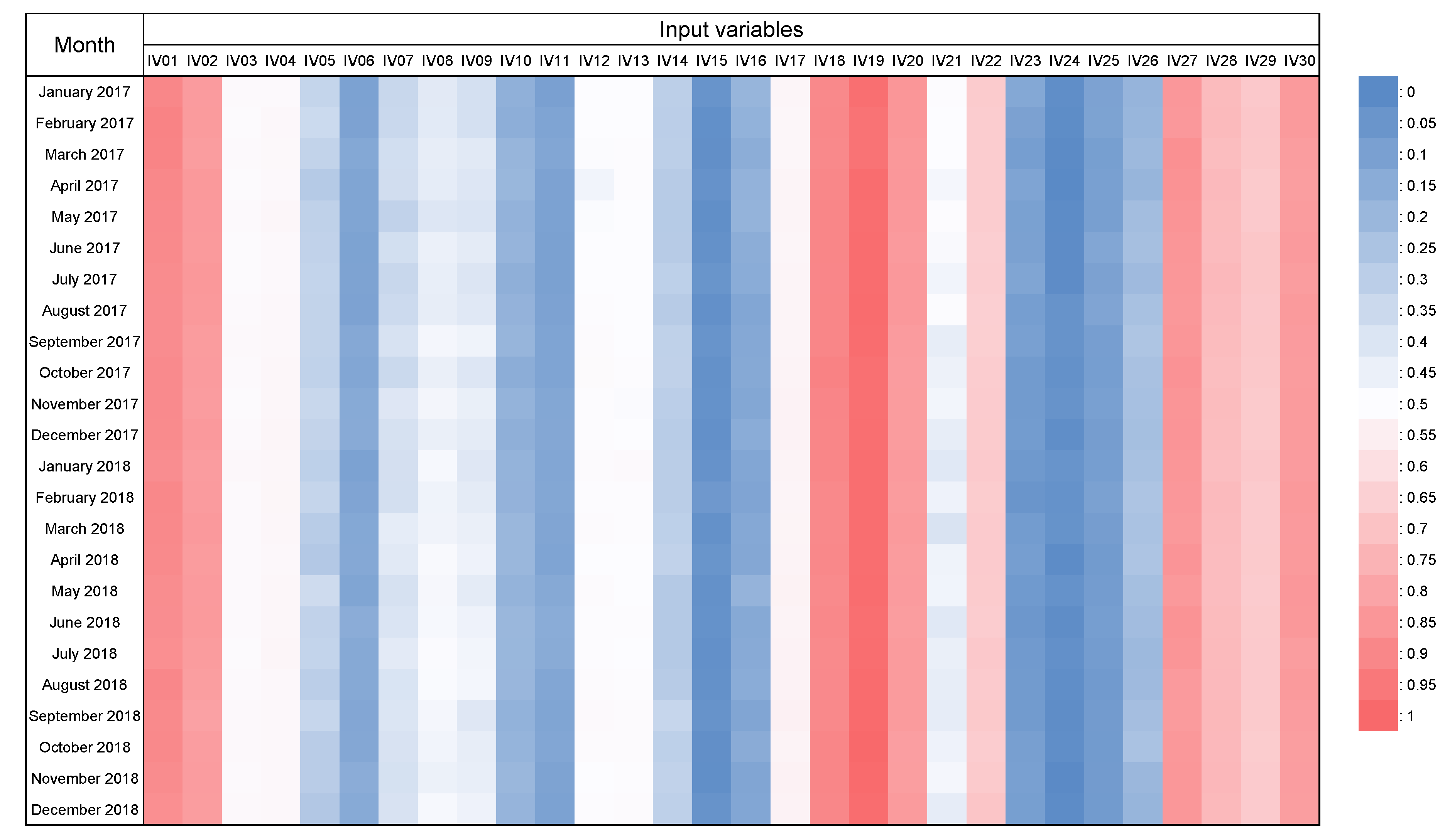
• We proposed an interpretable forecasting model based on feature importance analysis.
• We increased the accuracy of global solar radiation forecasting using TSCV.

This paper is organized as follows. In Section 2, we describe the overall process for constructing a LightGBM-based forecasting model for MSA global solar radiation forecasting. In Section 3, we analyze the experimental results and describe the interpretable forecasting results of our proposed model. Lastly, we discuss in Section 4 the conclusions and some future research directions.

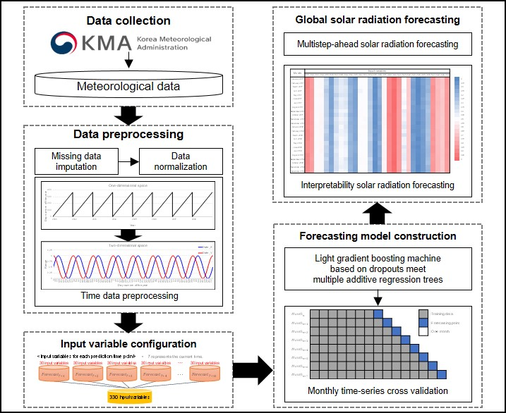
2. Materials and Methods

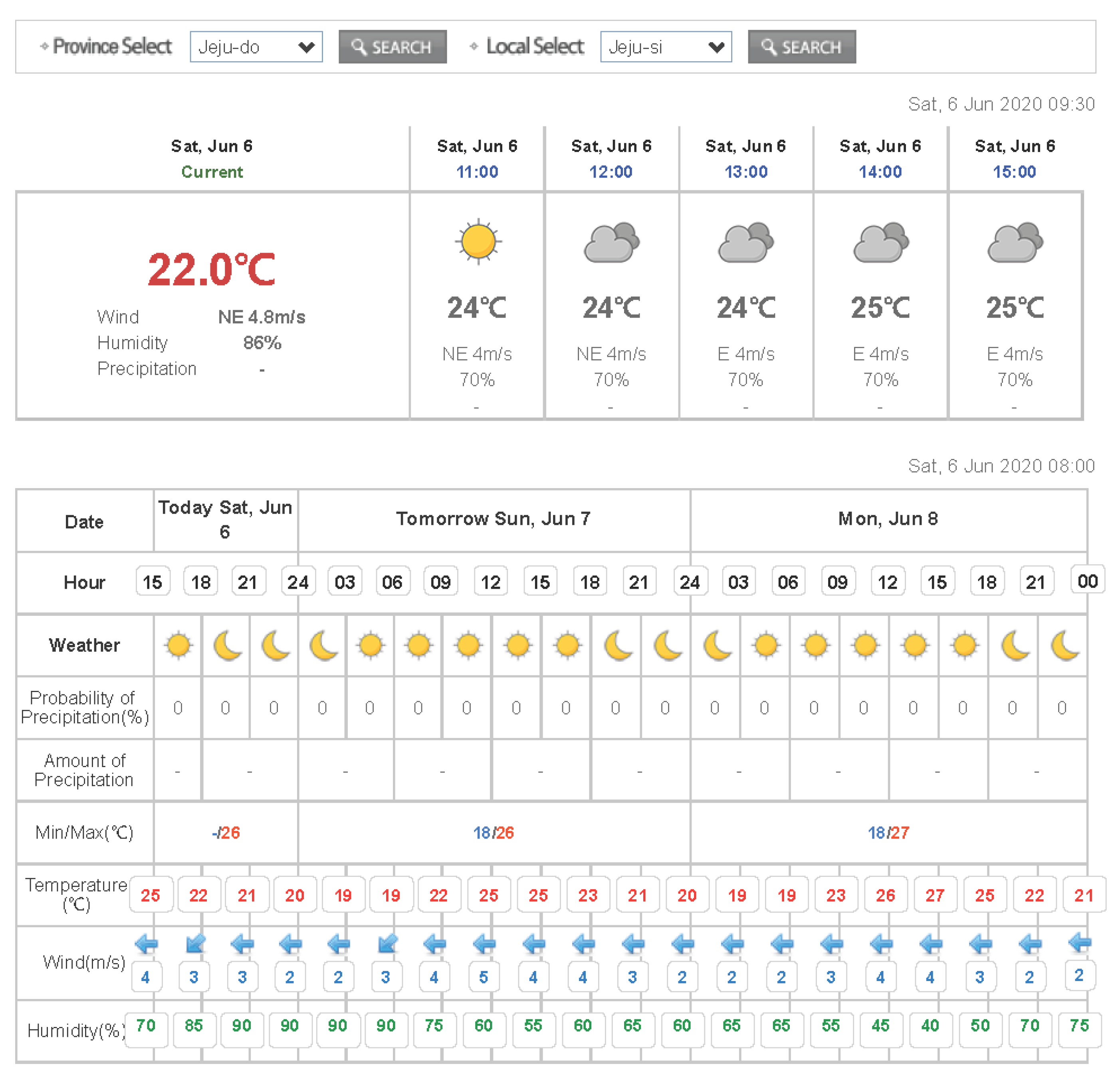
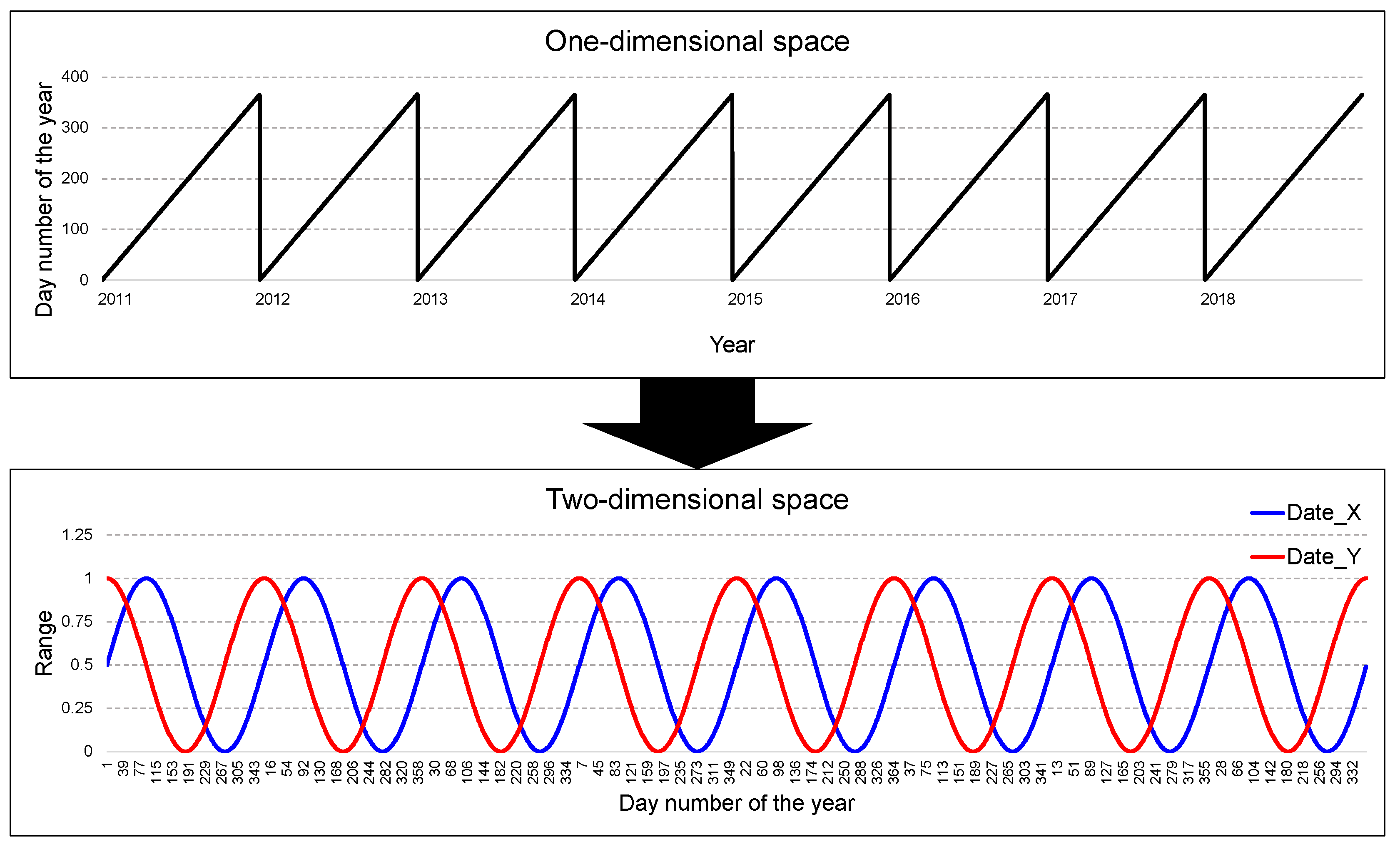
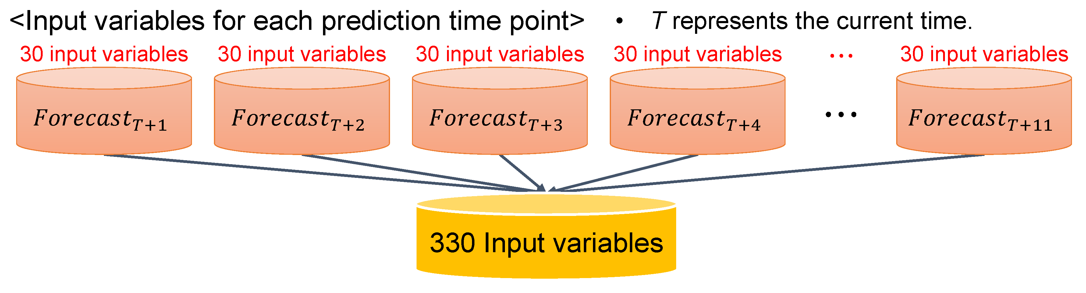
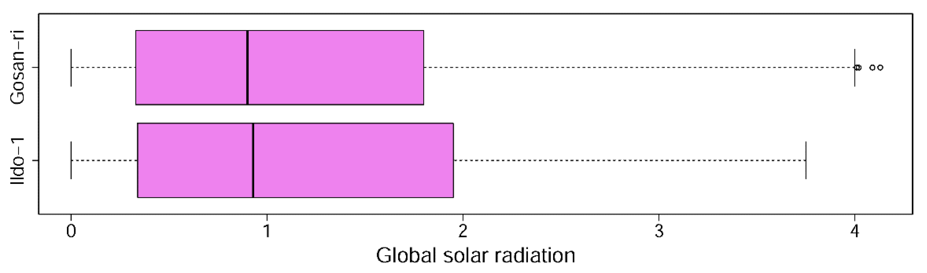
2.1. Data Collection and Preprocessing

In this paper, we used the date/time, meteorological data, and historical global solar radiation data provided by the KMA as input variables to construct a global solar radiation forecasting model. We considered two regions located on Jeju Island. Jeju is the largest island in South Korea and is implementing various measures to change into a smart island. For instance, it is enforcing diverse energy policies that encourage a shift from conventional fossil fuels to RESs. The two regions that we selected for validating prediction performance are Ildo-1 dong (latitude: 33.51411 and longitude: 126.52969) and Gosan-ri (latitude: 33.29382 and longitude: 126.16283). The data collection period is from 8 a.m. to 6 p.m. for a total of eight years from 2011 to 2018, and the collected data include temperature, humidity, wind speed, and global solar radiation. The meteorological observation data provided by the KMA include extra data, such as soil temperature, total cloud volume, ground-surface temperature, and sunshine amount. However, because the sky condition (also known as weather observation), temperature, humidity, and wind speed are provided by KMA’s short-term weather forecasts, as shown in Figure 1, we only considered these factors [24].

In the meteorological data we collected, about 0.1% of the total data for each category were missing, and the missing values were indicated as −1. Because the temperature, humidity, wind speed, and global solar radiation have continuous data characteristics, missing values can be estimated using linear interpolation. The sky condition data were presented as categorical values from 1 to 4, and missing values were approximated using logistic regression for similarity with the adjacent data.

For the date, to reflect the periodicity, one-dimensional data were augmented with continuous data in two-dimensional space using Equations (1) and (2) [25]. In the equations, end-of-month (EoM) indicates the last day of the month. The equations converted each Julian date into a value from 1 to 365. For instance, the Julian date of January 1 is converted to 1, and December 31 is converted to 365. In the case of leap years, 366 was used instead of 365 in the equations. Figure 2 illustrates an example of preprocessing the date data.

$$Dat{e}_X=\sin \left(360°\times ({{\displaystyle \sum }}_1^{Month-1}EoM+Day)/365\right)$$

(1)

$$Dat{e}_Y=\cos \left(360°\times ({{\displaystyle \sum }}_1^{Month-1}EoM+Day)/365\right)$$

(2)

The cloud amount is provided by the KMA. Of the two popular methods for representing cloud amount, which are meteorology 1/8 and climatology 1/10, the KMA uses the second method. Hence, the cloud amount is represented by eleven scales (i.e., from 0 for a clear sky to 10 for an overcast sky). The sky condition data have four interval scales [26,27]: 1 for clear (0 ≤ cloud amount ≤ 2), 2 for partly cloudy (3 ≤ cloud amount ≤ 5), 3 for mostly cloudy (6 ≤ cloud amount ≤ 8), and 4 for cloudy (9 ≤ cloud amount ≤ 10). Because we represent the sky condition data using one-hot encoding, a value of 1 is placed in the binary variable for a specific sky condition, and 0 is used for the other sky conditions. Time data were also represented by interval scales. Global solar radiation is highest during the day from 12 to 2 p.m. To assess these variables more effectively, we used one-hot encoding to represent time intervals.

In addition, to reflect the recent trends in global solar radiation, we used the sky condition, temperature, humidity, wind speed, and global solar radiation of the day before the forecast point as input variables. We considered 30 input variables to construct our prediction model, as shown in

Table 1. List of input variables (IV) for the proposed model.

IV #	Input Variable (Feature)	IV #	Input Variable (Feature)
IV01	$Dat{e}_X$ (numeric)	IV16	$Mostly cloudy$ (binary)
IV02	$Dat{e}_Y$ (numeric)	IV17	$Cloudy$ (binary)
IV03	$8 a.m.$ (binary)	IV18	$Temperature$ (numeric)
IV04	$9 a.m.$ (binary)	IV19	$Humidity$ (numeric)
IV05	$10 a.m.$ (binary)	IV20	$Wind speed$ (numeric)
IV06	$11 a.m.$ (binary)	IV21	$Dat{e}_X$ 1 day before (numeric)
IV07	$12 p.m.$ (binary)	IV22	$Dat{e}_Y$ 1 day before (numeric)
IV08	$1 p.m.$ (binary)	IV23	$Clear$ 1 day before (binary)
IV09	$2 p.m.$ (binary)	IV24	$Partly cloudy$ 1 day before (binary)
IV10	$3 p.m.$ (binary)	IV25	$Mostly cloudy$ 1 day before (binary)
IV11	$4 p.m.$ (binary)	IV26	$Cloudy$ 1 day before (binary)
IV12	$5 p.m.$ (binary)	IV27	$Temperature$ 1 day before (numeric)
IV13	$6 p.m.$ (binary)	IV28	$Humidity$ 1 day before (numeric)
IV14	$Clear$ (binary)	IV29	$Wind speed$ 1 day before (numeric)
IV15	$Partly cloudy$ (binary)	IV30	$Global solar radiation$ 1 day before (numeric)

. As our goal is to perform MSA (all time points for the next 24 h) forecasting, we needed all the input variables for 11 prediction time points. Therefore, we used 330 input variables (i.e., 30 input variables $\times$ 11 prediction time points) with 32,143 tuples for the MSA forecasting model construction, as shown in Figure 3.

2.2. Forecasting Model Construction

The purpose of our model is to predict global solar radiation for the next 11 time points from the current time. To construct a global solar radiation forecasting model, we used LightGBM, a gradient boosting machine (GBM)-based model. The LightGBM model [28] is based on a gradient boosting decision tree (GBDT) applying gradient-based one-side sampling and exclusive feature bundling technologies. Unlike the conventional GBM tree splitting method, a leafwise method is used to create complex models to achieve higher accuracy; hence, it is useful for time-series forecasting. Because of the GBDT and leafwise method, LightGBM has the advantages of reduced memory usage and faster training speed. The LightGBM contains various hyperparameters to be tuned. Among them, the learning rate, number of iterations, and number of leaves are closely related to the prediction accuracy. In addition, overfitting can be prevented by adjusting the colsample by tree and subsample hyperparameters. Moreover, LightGBM also can use different algorithms for its learning iterations. In this paper, we constructed two LightGBM models using two boosting types: GBDT and dropouts meet multiple additive regression trees (DART) [29] for comparison. Both models perform predictions on multiple outputs using the MultiOutputRegressor module in scikit-learn (v. 0.22.1).

In general, to evaluate a forecasting method, we first divide a dataset into training and test sets. Then, we construct the forecasting model using the training set. Finally, we evaluate the performance of the forecasting model using the test set. A greater time interval between training and forecasting lowers the prediction performance [30]. To solve this problem, we applied TSCV, which is popularly used when data exhibit time-series characteristics and are focused on a single forecast of the dataset [6]. The TSCV uses all data before the prediction point as a training set and predicts the next forecasting point by setting it as a test set, iteratively.

However, if TSCV is performed at every point, it requires a considerable amount of time to train and forecast. To reduce this overhead, we conducted monthly TSCV, as shown in Figure 4. In addition, for interpretable global solar radiation forecasting, we analyzed the variable importance changes for the 30 input variables by obtaining the feature importance using LightGBM.

2.3. Baseline Models

To demonstrate the performance of our model, we constructed various forecasting models based on the tree-based ensemble and deep learning methods.

In the case of tree-based ensemble learning methods, because they combine several weak models effectively, they usually exhibit better prediction performance than a single model. In the experiment, we considered RF, GBM, and extreme gradient boosting (XGBoost) ensemble methods to construct MSA global solar radiation forecasting models. The RF method trains each tree independently by using a randomly selected sample of the data. As the RF method tends to reduce the correlation between trees, it provides a robust model for out-of-sample forecasting [31]. In addition, the GBM is a forward-learning ensemble method that obtains predictive results using gradually improved estimations [32]. The adjusted model is built by applying the residuals of the previous model, and this procedure is repeated $N$ times to build a robust model. We constructed two GBM models by considering the quantile regression and Huber loss functions, respectively. The XGBoost method is an algorithm that can prevent overfitting by reducing the tree correlation using the shrinkage method [33]. Moreover, it can perform parallel processing by applying the column subsampling method. The XGBoost method constructs a weak model and evaluates the consistency using the training set. After that, the method constructs an adjusted prediction model with the explanatory variable for the gradient in the direction in which consistency increases using the gradient descent method. This procedure is repeated $N$ times to build a robust model [34]. We constructed two XGBoost models by applying two boosting types (i.e., GBDT and DART). To predict multiple outputs, we constructed an RF model using the MultivariateRandomForest [35] package in R (v. 3.5.1) and the GBM and XGBoost models using the MultiOutputRegressor module in scikit-learn (v. 0.22.1) [36].

For deep learning-based MSA global solar radiation forecasting models, we considered the SNN, DNN, LSTM network, and attention-based LSTM (ATT-LSTM) network. These models require a sufficient amount of training data for accurate predictive performance, and the models can overfit the data if the training data are insufficient [37]. A typical ANN consists of an input layer, one or more hidden layers, and an output layer, and each layer consists of one or more hidden nodes [38,39]. The ANNs have various hyperparameters that affect prediction performance [38]. These hyperparameters include the number of hidden layers, number of hidden nodes, an activation function, and so on. In addition, the SNN has one hidden layer, and the DNN has two or more hidden layers [39]. The LSTM network [40] is a model that can solve the long-term dependency problem of the existing recurrent neural network. The LSTM network is useful for training sequence data in the time-series forecasting method. Nevertheless, although the length of the input variable is long, the forecasting accuracy of the sequence-to-sequence model suffers due to focusing on all input variables. To solve this problem, an attention mechanism [41] has been developed in the field of machine translation. The attention mechanism comprises an encoder that builds a vector from the input variable and a decoder that outputs a dependent variable using the vector output by the encoder as input. The decoder part performs the model training focused on data representing high similarity by indicating the similarity with the encoder as a value; hence, it can exhibit accurate forecasting performance. Applying the attention mechanism to the LSTM described above focuses the model on specific vectors so that it obtains more accurate forecasting results [42].

In our previous work [7], we constructed several deep learning models for MSA global solar radiation forecasting in the same experimental environment. We used the dropout method to control the weight of the hidden layers to prevent overfitting. To do this, we found optimal hyperparameter values for each deep learning model, as indicated in

Table 2. Selected optimal hyperparameters for each deep learning model.

Models	Selected Hyperparameters
SNN	Number of hidden layers: 1 Number of hidden nodes: 14 Activation function: sigmoid Loss function: mean squared error Optimizer: Adam
DNN	Number of hidden layers: 7 Activation function: ReLU, SELU [43] Remaining hyperparameters are the same as those for the SNN model
LSTM network	Sequence length: 11 Number of hidden layers: 2 Activation function: ReLU, SELU [43] Loss function: Huber loss Optimizer: RMSProp Batch size: 11 Learning rate: 0.000001 Epoch: 5,000
ATT-LSTM network	Number of attention layers: 1 Remaining hyperparameters are the same as those for the LSTM network model

Notes: SNN: shallow neural network; DNN: deep neural network; LSTM: long short-term memory; ATT-LSTM: attention-based LSTM; ReLU: rectified linear unit; SELU: scaled exponential linear unit.

.

3. Results and Discussion

In the experiments, we used two global solar radiation datasets collected from two regions from 2011 to 2018. The two regions are Ildo-1 and Gosan-ri on Jeju island. We divided each dataset into two parts at a ratio of 75:25: a training set (in-sample) spanning 2011 to 2016, and a test set (out-of-sample) spanning 2017 to 2018.

Table 3. Statistical analysis of global solar radiation data by region ($\mathrm{MJ}/{\mathrm{m}}^2$).

Statistics	Ildo-1		Gosan-ri
	Training Set	Test Set	Training Set	Test Set
Mean	1.188	1.258	1.179	1.044
Standard error	0.006	0.011	0.006	0.009
Median	0.910	1.010	0.910	0.840
Mode	0	0	0	0
Standard deviation	0.995	1.000	0.989	0.842
Sample variance	0.990	1.000	0.979	0.710
Kurtosis	−0.756	−0.869	−0.400	−0.419
Skewness	0.659	0.568	0.764	0.713
Range	3.750	3.720	4.130	3.550
Minimum	0	0	0	0
Maximum	3.750	3.720	4.130	3.550
Sum	28,656.9	10,097.9	28,422.8	8383.9
Count	24,112	8030	24,112	8030

lists various statistical analysis for the datasets by considering the training and test sets. The statistical analysis was performed by using Excel’s Descriptive Statistics data analysis tool. Figure 5 represents the boxplots of the global solar radiation data for each region.

For continuous data, such as humidity, wind speed, temperature, and historical global solar radiation, we performed standardization using Equation (3). In the equation, x_i and x denote the input variable and original data, respectively. In addition, μ and σ denote the average of the original data and the standard deviation, respectively.

$$x_i=\frac{x-\mu }{\sigma }$$

(3)

To evaluate the prediction performance of the models, we used four metrics: mean biased error (MBE), mean absolute error (MAE), root mean square error (RMSE), and normalized root mean square error (NRMSE), as shown in Equations (4)–(7). Here, A_t and F_t represent the actual and forecasted values, respectively, at time t, n indicates the number of observations, and $\overline{A}$ represents the average of the actual values.

$$MBE=\frac{1}{n}{\displaystyle \sum }_{t=1}^n\left(A_t-F_t\right)$$

(4)

$$MAE=\frac{1}{n}{{\displaystyle \sum }}_{t=1}^n\left|F_t-A_t\right|$$

(5)

$$RMSE=\sqrt{\frac{{{\displaystyle \sum }}_{t=1}^n{\left(F_t-A_t\right)}^2}{n}}$$

(6)

$$NRMSE=\frac{\sqrt{\frac{{{\displaystyle \sum }}_{t=1}^n{\left(F_t-A_t\right)}^2}{n}}}{\overline{A}}\times 100$$

(7)

We implemented an RF-based forecasting model using R (v. 3.5.1) and all other forecasting models using Python (v. 3.6). We found optimal values for the hyperparameters of the tree-based ensemble learning models via GridSearchCV in scikit-learn (v. 0.22.1), as displayed in

Table 4. Selected hyperparameters for each ensemble learning model. Selected values are bold.

Models		Package or Module	Selected Hyperparameters
Random forest		MultivariateRandomForest	Number of trees: 128 [44] Number of features: 110 [44]
GBM	Quantile regression	GradientBoostingRegressor GridSearchCV	Learning rate: 0.01, 0.05, 0.1 Number of iterations: 100, 250, 500 Maximum depth of the tree: 5, 10
	Huber loss		Learning rate: 0.01, 0.05, 0.1 Number of iterations: 100, 250, 500 Maximum depth of the tree: 5, 10
XGBoost	GBDT	XGBoost 1.0.2 GridSearchCV	Learning rate: 0.01, 0.05, 0.1 Number of iterations: 250, 500, 1000 Maximum depth of the tree: 6, 8, 10 Subsample: 0.5, 0.75, 1.0 Colsample by tree: 0.5, 0.75, 1.0 Colsample by level: 0.5, 0.75, 1.0 Colsample by node: 0.5, 0.75, 1.0
	DART		Learning rate: 0.01, 0.05, 0.1 Number of iterations: 250, 500, 1000 Maximum depth of the tree: 6, 8, 10 Subsample: 0.5, 0.75, 1.0 Colsample by tree: 0.5, 0.75, 1.0 Colsample by level: 0.5, 0.75, 1.0 Colsample by node: 0.5, 0.75, 1.0
LightGBM	GBDT	LightGBM 2.3.1 GridSearchCV	Learning rate: 0.01, 0.05, 0.1 Number of iterations: 1000, 1500 Number of leaves: 64 Subsample: 0.5 Colsample by tree: 1.0
	DART (our model)		Learning rate: 0.01, 0.05, 0.1 Number of iterations: 1000, 1500 Number of leaves: 64 Subsample: 0.5 Colsample by tree: 1.0

Notes: GBM: gradient boosting machine; XGBoost: extreme gradient boosting; LightGBM: light GBM; GBDT: gradient boosting decision tree; DART: dropouts meet multiple additive regression trees.

. Because the two regions are close together, we obtained the same hyperparameter values for the two regions.

Table 5. Mean bias error (MBE) distribution for each model for Ildo-1 ($\mathrm{MJ}/{\mathrm{m}}^2$).

Models	Points
	1	2	3	4	5	6	7	8	9	10	11
SNN (Dropout O)	−0.05	−0.04	−0.03	−0.03	−0.03	−0.05	−0.06	−0.07	−0.07	−0.06	−0.04
SNN (Dropout X)	−0.04	−0.01	−0.04	−0.05	−0.05	−0.05	−0.04	−0.04	−0.04	−0.04	−0.04
DNN-ReLU (Dropout O)	−0.04	0	−0.06	−0.07	−0.08	−0.09	−0.10	−0.12	−0.13	−0.13	−0.14
DNN-ReLU (Dropout X)	−0.06	−0.06	−0.07	−0.07	−0.08	−0.08	−0.08	−0.08	−0.08	−0.07	−0.06
DNN-SELU (Dropout O)	0.05	0.08	0.02	−0.03	−0.04	−0.05	−0.03	0	−0.03	−0.02	−0.02
DNN-SELU (Dropout X)	−0.06	−0.06	−0.09	−0.10	−0.10	−0.10	−0.10	−0.10	−0.10	−0.10	−0.11
LSTM-ReLU (Dropout O)	−0.10	0.05	−0.02	−0.06	−0.06	−0.05	−0.04	−0.02	−0.02	−0.02	−0.23
LSTM-ReLU (Dropout X)	−0.19	−0.01	−0.02	−0.06	−0.10	−0.12	−0.12	−0.11	−0.10	−0.09	−0.08
LSTM-SELU (Dropout O)	−0.09	−0.02	−0.06	−0.07	−0.06	−0.04	−0.03	−0.03	−0.02	−0.03	−0.03
LSTM-SELU (Dropout X)	−0.10	−0.03	−0.06	−0.09	−0.10	−0.09	−0.09	−0.09	−0.09	−0.09	−0.09
ATT−LSTM-RELU (Dropout O)	−0.16	−0.14	−0.09	−0.07	−0.07	−0.01	0.02	0.03	0.01	−0.05	−0.09
ATT−LSTM-RELU (Dropout X)	−0.14	−0.11	−0.11	−0.06	0	0.09	0.07	0.09	0.12	0.01	−0.02
ATT−LSTM-SELU (Dropout O)	−0.04	0.02	−0.06	0.01	0.04	−0.06	−0.10	0	0.03	−0.02	−0.03
ATT−LSTM-SELU (Dropout X)	0.13	0.13	0.08	−0.05	−0.11	−0.18	−0.25	−0.18	−0.29	−0.30	−0.20
RF (TSCV)	−0.03	−0.04	−0.05	−0.06	−0.07	−0.07	−0.07	−0.07	−0.07	−0.06	−0.06
RF (Holdout)	−0.04	−0.05	−0.07	−0.08	−0.09	−0.09	−0.09	−0.09	−0.08	−0.08	−0.08
GBM-Huber (TSCV)	−0.02	−0.03	−0.04	−0.05	−0.05	−0.05	−0.05	−0.04	−0.04	−0.04	−0.03
GBM-Huber (Holdout)	−0.03	−0.04	−0.05	−0.07	−0.07	−0.07	−0.07	−0.06	−0.06	−0.05	−0.04
GBM-Quantile (TSCV)	0.24	0.32	0.35	0.38	0.39	0.41	0.42	0.43	0.45	0.45	0.46
GBM-Quantile (Holdout)	0.24	0.31	0.34	0.36	0.38	0.39	0.40	0.42	0.44	0.45	0.46
XGBoost-GDBT (TSCV)	−0.02	−0.03	−0.05	−0.05	−0.05	−0.05	−0.05	−0.05	−0.05	−0.04	−0.04
XGBoost-GDBT (Holdout)	−0.03	−0.05	−0.06	−0.07	−0.08	−0.07	−0.07	−0.07	−0.07	−0.06	−0.06
XGBoost-DART (TSCV)	−0.02	−0.03	−0.04	−0.05	−0.05	−0.05	−0.05	−0.05	−0.05	−0.04	−0.04
XGBoost-DART (Holdout)	−0.03	−0.05	−0.06	−0.07	−0.08	−0.07	−0.07	−0.07	−0.06	−0.06	−0.06
LightGBM-GDBT (TSCV)	−0.02	−0.03	−0.04	−0.04	−0.05	−0.05	−0.05	−0.05	−0.04	−0.05	−0.05
LightGBM-GDBT (Holdout)	−0.03	−0.05	−0.06	−0.07	−0.07	−0.08	−0.08	−0.07	−0.07	−0.08	−0.07
LightGBM-DART (TSCV)	−0.03	−0.04	−0.05	−0.06	−0.06	−0.06	−0.06	−0.05	−0.05	−0.05	−0.05
LightGBM-DART (Holdout)	−0.04	−0.06	−0.07	−0.08	−0.08	−0.08	−0.08	−0.07	−0.07	−0.07	−0.06

,

Table 6. Mean absolute error (MAE) distribution for each model for Ildo-1. A cooler color indicates a lower MAE value, whereas a warmer color indicates a higher MAE value ($\mathrm{MJ}/{\mathrm{m}}^2$).

Models	Points
	1	2	3	4	5	6	7	8	9	10	11
SNN (Dropout O)	0.445	0.406	0.394	0.390	0.386	0.385	0.385	0.386	0.385	0.385	0.385
SNN (Dropout X)	0.413	0.390	0.393	0.392	0.390	0.388	0.387	0.387	0.388	0.391	0.395
DNN-ReLU (Dropout O)	0.419	0.384	0.389	0.386	0.382	0.379	0.380	0.382	0.385	0.388	0.391
DNN-ReLU (Dropout X)	0.445	0.401	0.398	0.387	0.384	0.385	0.383	0.381	0.381	0.381	0.381
DNN-SELU (Dropout O)	0.349	0.327	0.343	0.354	0.363	0.368	0.375	0.382	0.395	0.395	0.405
DNN-SELU (Dropout X)	0.408	0.383	0.380	0.378	0.376	0.374	0.373	0.373	0.374	0.376	0.378
LSTM-ReLU (Dropout O)	0.365	0.388	0.409	0.412	0.420	0.427	0.436	0.436	0.446	0.458	0.460
LSTM-ReLU (Dropout X)	0.380	0.399	0.417	0.426	0.431	0.442	0.456	0.467	0.468	0.470	0.470
LSTM-SELU (Dropout O)	0.318	0.332	0.350	0.360	0.372	0.377	0.371	0.373	0.378	0.379	0.370
LSTM-SELU (Dropout X)	0.357	0.379	0.400	0.412	0.413	0.438	0.446	0.467	0.488	0.501	0.517
ATT-LSTM-RELU (Dropout O)	0.291	0.324	0.329	0.340	0.347	0.348	0.357	0.363	0.368	0.382	0.394
ATT-LSTM-RELU (Dropout X)	0.272	0.299	0.324	0.332	0.339	0.351	0.349	0.360	0.375	0.378	0.392
ATT-LSTM-SELU (Dropout O)	0.238	0.291	0.311	0.330	0.333	0.346	0.368	0.348	0.358	0.371	0.381
ATT-LSTM-SELU (Dropout X)	0.261	0.301	0.307	0.319	0.343	0.376	0.414	0.386	0.439	0.452	0.415
RF (TSCV)	0.215	0.272	0.306	0.330	0.347	0.363	0.375	0.388	0.401	0.414	0.428
RF (Holdout)	0.223	0.280	0.315	0.340	0.358	0.371	0.383	0.396	0.409	0.423	0.435
GBM-Huber (TSCV)	0.186	0.251	0.292	0.318	0.337	0.351	0.359	0.368	0.374	0.382	0.385
GBM-Huber (Holdout)	0.189	0.257	0.300	0.330	0.350	0.359	0.370	0.377	0.383	0.392	0.394
GBM-Quantile (TSCV)	0.288	0.376	0.418	0.445	0.462	0.476	0.484	0.498	0.511	0.518	0.525
GBM-Quantile (Holdout)	0.287	0.375	0.413	0.445	0.461	0.470	0.482	0.497	0.510	0.524	0.530
XGBoost-GDBT (TSCV)	0.194	0.257	0.296	0.324	0.339	0.348	0.356	0.366	0.375	0.384	0.390
XGBoost-GDBT (Holdout)	0.197	0.263	0.305	0.333	0.349	0.358	0.367	0.374	0.383	0.390	0.396
XGBoost-DART (TSCV)	0.184	0.249	0.289	0.317	0.333	0.346	0.353	0.362	0.369	0.377	0.382
XGBoost-DART (Holdout)	0.188	0.255	0.298	0.328	0.346	0.357	0.364	0.372	0.379	0.386	0.393
LightGBM-GDBT (TSCV)	0.189	0.253	0.292	0.319	0.334	0.348	0.355	0.363	0.371	0.377	0.381
LightGBM-GDBT (Holdout)	0.193	0.261	0.305	0.331	0.346	0.359	0.368	0.373	0.382	0.391	0.394
LightGBM-DART (TSCV)	0.189	0.252	0.290	0.318	0.333	0.344	0.350	0.358	0.365	0.374	0.380
LightGBM-DART (Holdout)	0.193	0.257	0.300	0.328	0.344	0.355	0.359	0.369	0.377	0.384	0.389

,

Table 7. Root mean square error (RMSE) distribution for each model for Ildo-1. A cooler color indicates a lower RMSE value, whereas a warmer color indicates a higher RMSE value ($\mathrm{MJ}/{\mathrm{m}}^2$).

Models	Points
	1	2	3	4	5	6	7	8	9	10	11
SNN (Dropout O)	0.588	0.546	0.537	0.534	0.528	0.526	0.524	0.525	0.524	0.525	0.528
SNN (Dropout X)	0.545	0.532	0.534	0.533	0.529	0.526	0.524	0.524	0.526	0.529	0.534
DNN-ReLU (Dropout O)	0.545	0.528	0.529	0.525	0.519	0.514	0.513	0.515	0.519	0.523	0.527
DNN-ReLU (Dropout X)	0.598	0.548	0.545	0.525	0.520	0.518	0.515	0.514	0.513	0.514	0.515
DNN-SELU (Dropout O)	0.392	0.441	0.465	0.479	0.487	0.499	0.506	0.508	0.522	0.519	0.532
DNN-SELU (Dropout X)	0.541	0.526	0.523	0.512	0.515	0.511	0.509	0.509	0.510	0.511	0.514
LSTM-ReLU (Dropout O)	0.544	0.547	0.545	0.541	0.540	0.540	0.547	0.551	0.559	0.570	0.636
LSTM-ReLU (Dropout X)	0.545	0.550	0.543	0.544	0.500	0.543	0.550	0.551	0.558	0.567	0.637
LSTM-SELU (Dropout O)	0.408	0.448	0.462	0.473	0.484	0.494	0.506	0.516	0.517	0.518	0.519
LSTM-SELU (Dropout X)	0.431	0.467	0.481	0.492	0.506	0.507	0.521	0.531	0.551	0.551	0.558
ATT-LSTM-RELU (Dropout O)	0.381	0.430	0.446	0.464	0.478	0.481	0.491	0.499	0.505	0.515	0.528
ATT-LSTM-RELU (Dropout X)	0.383	0.428	0.458	0.466	0.475	0.496	0.498	0.512	0.529	0.530	0.543
ATT-LSTM-SELU (Dropout O)	0.329	0.395	0.431	0.455	0.464	0.479	0.502	0.493	0.508	0.519	0.528
ATT-LSTM-SELU (Dropout X)	0.357	0.415	0.431	0.450	0.475	0.509	0.557	0.538	0.586	0.598	0.561
RF (TSCV)	0.302	0.378	0.421	0.450	0.471	0.490	0.504	0.516	0.528	0.540	0.554
RF (Holdout)	0.308	0.386	0.431	0.462	0.484	0.502	0.515	0.527	0.538	0.550	0.564
GBM-Huber (TSCV)	0.285	0.369	0.417	0.451	0.472	0.490	0.498	0.507	0.513	0.518	0.520
GBM-Huber (Holdout)	0.288	0.376	0.427	0.465	0.490	0.501	0.514	0.521	0.526	0.530	0.533
GBM-Quantile (TSCV)	0.412	0.527	0.594	0.638	0.663	0.682	0.695	0.714	0.732	0.739	0.749
GBM-Quantile (Holdout)	0.409	0.523	0.584	0.637	0.660	0.671	0.689	0.706	0.727	0.739	0.751
XGBoost-GDBT (TSCV)	0.289	0.371	0.417	0.452	0.471	0.484	0.494	0.504	0.511	0.517	0.521
XGBoost-GDBT (Holdout)	0.290	0.376	0.427	0.466	0.485	0.498	0.508	0.514	0.520	0.523	0.528
XGBoost-DART (TSCV)	0.280	0.363	0.410	0.444	0.466	0.481	0.491	0.499	0.504	0.509	0.514
XGBoost-DART (Holdout)	0.283	0.369	0.421	0.460	0.483	0.498	0.508	0.513	0.519	0.522	0.527
LightGBM-GDBT (TSCV)	0.285	0.368	0.415	0.449	0.469	0.488	0.496	0.507	0.512	0.515	0.520
LightGBM-GDBT (Holdout)	0.289	0.377	0.431	0.466	0.485	0.504	0.514	0.519	0.526	0.532	0.537
LightGBM-DART (TSCV)	0.284	0.366	0.411	0.444	0.464	0.479	0.487	0.496	0.502	0.508	0.514
LightGBM-DART (Holdout)	0.288	0.370	0.421	0.459	0.482	0.494	0.502	0.511	0.518	0.523	0.525

,

Table 8. Normalized root mean square error (NRMSE) distribution for each model for Ildo-1. A cooler color indicates a lower NRMSE value, whereas a warmer color indicates a higher NRMSE value ($\%$).

Models	Points
	1	2	3	4	5	6	7	8	9	10	11
SNN (Dropout O)	46.6	43.3	42.6	42.4	41.9	41.7	41.6	41.6	41.5	41.6	41.8
SNN (Dropout X)	42.9	41.7	41.4	41.1	40.8	40.5	40.3	40.3	40.4	40.5	40.7
DNN-ReLU (Dropout O)	43.6	41.9	42.0	41.6	41.1	40.8	40.7	40.9	41.1	41.4	41.8
DNN-ReLU (Dropout X)	47.4	43.5	42.4	41.7	41.2	41.0	40.8	40.7	40.7	40.7	40.8
DNN-SELU (Dropout O)	31.2	35.0	36.9	38.0	38.7	39.7	40.2	40.4	41.5	41.3	42.2
DNN-SELU (Dropout X)	43.2	42.2	42.4	42.2	42.0	41.7	41.5	41.5	41.7	41.9	42.4
LSTM-ReLU (Dropout O)	48.2	43.5	42.4	42.1	41.8	41.4	41.1	40.9	40.8	41.0	41.2
LSTM-ReLU (Dropout X)	55.9	48.7	47.2	46.5	46.1	45.9	45.5	45.8	45.3	45.4	45.6
LSTM-SELU (Dropout O)	46.7	43.1	42.3	41.6	41.2	40.9	40.8	40.9	41.1	41.3	41.5
LSTM-SELU (Dropout X)	50.5	45.0	44.3	44.0	43.9	43.7	43.1	43.3	43.5	43.7	43.9
ATT-LSTM-RELU (Dropout O)	30.2	34.2	35.4	36.9	37.9	38.2	39.0	39.6	40.1	40.9	41.9
ATT-LSTM-RELU (Dropout X)	30.4	34.0	36.3	37.0	37.7	39.4	39.5	40.7	42.0	42.1	43.1
ATT-LSTM-SELU (Dropout O)	26.1	31.4	34.2	36.1	36.8	38.0	39.8	39.1	40.3	41.2	42.0
ATT-LSTM-SELU (Dropout X)	28.3	32.9	34.2	35.8	37.7	40.4	44.2	42.7	46.6	47.6	44.5
RF (TSCV)	24.0	30.0	33.4	35.7	37.4	38.9	40.1	41.0	42.0	43.0	44.1
RF (Holdout)	24.5	30.7	34.3	36.7	38.5	39.9	41.0	41.9	42.8	43.8	44.8
GBM-Huber (TSCV)	22.6	29.3	33.1	35.8	37.5	38.9	39.6	40.3	40.8	41.2	41.4
GBM-Huber (Holdout)	22.8	29.9	33.9	36.9	39.0	39.8	40.9	41.4	41.8	42.1	42.3
GBM-Quantile (TSCV)	32.7	41.9	47.2	50.7	52.7	54.2	55.2	56.7	58.2	58.8	59.5
GBM-Quantile (Holdout)	32.5	41.6	46.4	50.6	52.4	53.4	54.8	56.2	57.8	58.8	59.7
XGBoost-GDBT (TSCV)	22.9	29.4	33.1	35.9	37.4	38.5	39.3	40.1	40.6	41.1	41.4
XGBoost-GDBT (Holdout)	23.1	29.9	33.9	37.0	38.5	39.6	40.3	40.8	41.4	41.6	42.0
XGBoost-DART (TSCV)	22.3	28.9	32.6	35.3	37.0	38.2	39.0	39.7	40.1	40.5	40.8
XGBoost-DART (Holdout)	22.5	29.3	33.5	36.5	38.4	39.6	40.4	40.8	41.3	41.5	41.9
LightGBM-GDBT (TSCV)	22.7	29.3	33.0	35.7	37.2	38.8	39.5	40.3	40.7	40.9	41.4
LightGBM-GDBT (Holdout)	23.0	29.9	34.2	37.0	38.5	40.0	40.9	41.2	41.8	42.3	42.7
LightGBM-DART (TSCV)	22.5	29.1	32.7	35.3	36.9	38.1	38.7	39.4	39.9	40.4	40.9
LightGBM-DART (Holdout)	22.9	29.4	33.5	36.5	38.3	39.3	39.9	40.6	41.1	41.6	41.8

,

Table 9. Mean bias error (MBE) distribution for each model of Gosan-ri ($\mathrm{MJ}/{\mathrm{m}}^2$).

Models	Points
	1	2	3	4	5	6	7	8	9	10	11
SNN (Dropout O)	−0.04	−0.01	−0.02	−0.02	−0.02	−0.02	−0.02	−0.02	−0.02	−0.02	−0.02
SNN (Dropout X)	0.01	0.01	−0.01	−0.02	−0.02	−0.02	−0.01	0	0	0.01	0.02
DNN-ReLU (Dropout O)	−0.01	0	0.01	0.02	0.02	0.02	0.02	0.02	0.02	0.03	0.03
DNN-ReLU (Dropout X)	0.04	0.07	0.05	0.04	0.03	0.03	0.04	0.04	0.04	0.04	0.04
DNN-SELU (Dropout O)	0.04	0.06	0.07	0.06	0.04	0.05	0.05	0.06	0.06	−0.01	−0.01
DNN-SELU (Dropout X)	−0.02	0.02	0.01	−0.02	−0.03	−0.04	−0.04	−0.04	−0.05	−0.05	−0.05
LSTM-ReLU (Dropout O)	−0.13	0.08	0.08	0.05	0.02	−0.01	−0.01	−0.01	0.01	0.03	0.04
LSTM-ReLU (Dropout X)	−0.16	0.02	0.03	0	−0.03	−0.05	−0.05	−0.05	−0.40	−0.03	−0.02
LSTM-SELU (Dropout O)	0	0.03	0	−0.02	−0.04	−0.04	−0.04	−0.04	−0.04	−0.04	−0.04
LSTM-SELU (Dropout X)	−0.05	0.04	0.02	0	−0.02	−0.03	−0.03	−0.03	−0.02	−0.02	−0.02
ATT-LSTM-RELU (Dropout O)	0.02	−0.07	−0.01	0.03	0.04	0.13	0.16	0.10	−0.02	0.06	0
ATT-LSTM-RELU (Dropout X)	−0.05	−0.09	−0.08	−0.16	−0.24	−0.20	−0.25	−0.15	−0.24	−0.28	−0.25
ATT-LSTM-SELU (Dropout O)	0.05	0.05	0.01	−0.02	−0.01	0.01	−0.08	−0.11	−0.14	−0.06	−0.02
ATT-LSTM-SELU (Dropout X)	−0.04	−0.06	−0.01	−0.02	−0.04	−0.02	−0.02	0	−0.01	0.03	−0.01
RF (TSCV)	0	0	0	0	0	0	0	0.01	0.01	0.02	0.02
RF (Holdout)	0	0	0	0	0	0	0.01	0.01	0.02	0.02	0.03
GBM-Huber (TSCV)	−0.01	−0.01	−0.01	−0.01	−0.01	0	0	0	0	0	0
GBM-Huber (Holdout)	−0.01	−0.01	−0.01	−0.01	−0.01	0	0.01	0.01	0.01	0.01	0.01
GBM-Quantile (TSCV)	0.37	0.46	0.53	0.58	0.60	0.62	0.63	0.65	0.66	0.67	0.68
GBM-Quantile (Holdout)	0.26	0.32	0.36	0.39	0.42	0.41	0.43	0.44	0.45	0.47	0.46
XGBoost-GDBT (TSCV)	−0.01	−0.01	−0.01	−0.01	−0.01	−0.01	−0.01	0	−0.01	0	0
XGBoost-GDBT (Holdout)	−0.01	−0.01	−0.01	−0.01	−0.01	−0.01	0	0	0	0	0
XGBoost-DART (TSCV)	0	−0.01	−0.01	−0.01	0	0	0	0	0	0	0
XGBoost-DART (Holdout)	0	−0.01	0	0	0	0.01	0.01	0.01	0.01	0.01	0.01
LightGBM-GDBT (TSCV)	−0.01	−0.01	0	0	0	0	0	0	0	0	0
LightGBM-GDBT (Holdout)	0	−0.01	0	0	0.01	0.01	0.01	0.01	0.01	0.01	0.01
LightGBM-DART (TSCV)	−0.01	−0.02	−0.01	−0.01	−0.01	−0.01	−0.01	0	−0.01	0	0
LightGBM-DART (Holdout)	−0.01	−0.02	−0.01	−0.01	−0.01	0	0.01	0	0	0	0

,

Table 10. Mean absolute error (MAE) distribution for each model of Gosan-ri. A cooler color indicates a lower MAE value, whereas a warmer color indicates a higher MAE value ($\mathrm{MJ}/{\mathrm{m}}^2$).

Models	Points
	1	2	3	4	5	6	7	8	9	10	11
SNN (Dropout O)	0.426	0.399	0.391	0.387	0.381	0.377	0.373	0.374	0.375	0.374	0.373
SNN (Dropout X)	0.388	0.375	0.374	0.370	0.364	0.360	0.358	0.357	0.357	0.356	0.355
DNN-ReLU (Dropout O)	0.409	0.381	0.377	0.373	0.370	0.369	0.367	0.367	0.369	0.367	0.374
DNN-ReLU (Dropout X)	0.421	0.399	0.387	0.394	0.384	0.379	0.371	0.388	0.401	0.399	0.389
DNN-SELU (Dropout O)	0.278	0.306	0.325	0.343	0.355	0.365	0.367	0.379	0.388	0.387	0.397
DNN-SELU (Dropout X)	0.409	0.381	0.380	0.375	0.370	0.367	0.364	0.363	0.365	0.367	0.367
LSTM-ReLU (Dropout O)	0.345	0.358	0.359	0.362	0.370	0.377	0.386	0.376	0.376	0.378	0.380
LSTM-ReLU (Dropout X)	0.377	0.399	0.401	0.408	0.415	0.420	0.422	0.421	0.421	0.421	0.420
LSTM-SELU (Dropout O)	0.298	0.312	0.320	0.340	0.352	0.367	0.371	0.383	0.388	0.389	0.390
LSTM-SELU (Dropout X)	0.340	0.351	0.352	0.357	0.360	0.361	0.369	0.372	0.371	0.371	0.371
ATT-LSTM-RELU (Dropout O)	0.221	0.265	0.289	0.317	0.332	0.365	0.377	0.365	0.366	0.371	0.373
ATT-LSTM-RELU (Dropout X)	0.240	0.295	0.311	0.346	0.385	0.383	0.409	0.384	0.416	0.445	0.442
ATT-LSTM-SELU (Dropout O)	0.219	0.262	0.289	0.316	0.327	0.340	0.354	0.363	0.376	0.378	0.383
ATT-LSTM-SELU (Dropout X)	0.231	0.273	0.297	0.310	0.327	0.338	0.347	0.359	0.367	0.376	0.380
RF (TSCV)	0.176	0.227	0.256	0.277	0.293	0.307	0.319	0.331	0.343	0.353	0.363
RF (Holdout)	0.180	0.230	0.260	0.280	0.297	0.310	0.324	0.335	0.346	0.356	0.364
GBM-Huber (TSCV)	0.164	0.224	0.259	0.284	0.302	0.314	0.323	0.330	0.340	0.347	0.352
GBM-Huber (Holdout)	0.165	0.226	0.264	0.290	0.306	0.316	0.324	0.334	0.340	0.350	0.355
GBM-Quantile (TSCV)	0.289	0.359	0.410	0.453	0.468	0.481	0.492	0.505	0.510	0.522	0.530
GBM-Quantile (Holdout)	0.297	0.367	0.418	0.457	0.484	0.483	0.504	0.511	0.523	0.541	0.534
XGBoost-GDBT (TSCV)	0.168	0.222	0.254	0.280	0.295	0.306	0.314	0.324	0.334	0.341	0.346
XGBoost-GDBT (Holdout)	0.170	0.224	0.258	0.285	0.299	0.308	0.316	0.325	0.334	0.343	0.349
XGBoost-DART (TSCV)	0.159	0.216	0.249	0.275	0.291	0.302	0.312	0.321	0.329	0.339	0.345
XGBoost-DART (Holdout)	0.161	0.220	0.255	0.281	0.296	0.307	0.316	0.325	0.333	0.341	0.348
LightGBM-GDBT (TSCV)	0.167	0.225	0.259	0.283	0.300	0.312	0.320	0.331	0.336	0.343	0.353
LightGBM-GDBT (Holdout)	0.169	0.228	0.265	0.290	0.305	0.316	0.325	0.336	0.343	0.348	0.355
LightGBM-DART (TSCV)	0.163	0.218	0.252	0.276	0.293	0.304	0.314	0.322	0.332	0.341	0.347
LightGBM-DART (Holdout)	0.165	0.222	0.259	0.283	0.297	0.311	0.318	0.328	0.336	0.344	0.352

,

Table 11. Root mean square error (RMSE) distribution for each model for Gosan-ri. A cooler color indicates a lower RMSE value, whereas a warmer color indicates a higher RMSE value ($\mathrm{MJ}/{\mathrm{m}}^2$).

Models	Points
	1	2	3	4	5	6	7	8	9	10	11
SNN (Dropout O)	0.559	0.533	0.528	0.531	0.530	0.527	0.525	0.526	0.523	0.522	0.521
SNN (Dropout X)	0.518	0.518	0.520	0.517	0.512	0.506	0.502	0.501	0.499	0.497	0.497
DNN-ReLU (Dropout O)	0.522	0.519	0.519	0.512	0.506	0.500	0.496	0.495	0.495	0.496	0.497
DNN-ReLU (Dropout X)	0.552	0.522	0.523	0.522	0.520	0.520	0.521	0.521	0.521	0.522	0.526
DNN-SELU (Dropout O)	0.366	0.407	0.431	0.452	0.469	0.484	0.490	0.503	0.516	0.514	0.524
DNN-SELU (Dropout X)	0.532	0.519	0.521	0.517	0.514	0.511	0.509	0.509	0.510	0.511	0.511
LSTM-ReLU (Dropout O)	0.400	0.420	0.437	0.442	0.451	0.462	0.473	0.488	0.501	0.511	0.511
LSTM-ReLU (Dropout X)	0.455	0.462	0.477	0.484	0.491	0.500	0.511	0.531	0.547	0.567	0.580
LSTM-SELU (Dropout O)	0.375	0.380	0.410	0.444	0.467	0.486	0.492	0.510	0.526	0.533	0.538
LSTM-SELU (Dropout X)	0.406	0.417	0.451	0.471	0.490	0.496	0.500	0.508	0.522	0.547	0.555
ATT-LSTM-RELU (Dropout O)	0.306	0.370	0.403	0.435	0.454	0.485	0.497	0.495	0.508	0.515	0.517
ATT-LSTM-RELU (Dropout X)	0.338	0.416	0.445	0.490	0.541	0.539	0.569	0.527	0.566	0.586	0.581
ATT-LSTM-SELU (Dropout O)	0.297	0.360	0.401	0.436	0.452	0.473	0.500	0.515	0.529	0.524	0.526
ATT-LSTM-SELU (Dropout X)	0.322	0.380	0.415	0.432	0.456	0.470	0.485	0.499	0.511	0.522	0.524
RF (TSCV)	0.257	0.322	0.359	0.387	0.409	0.426	0.441	0.457	0.470	0.481	0.490
RF (Holdout)	0.260	0.326	0.364	0.391	0.413	0.431	0.449	0.464	0.475	0.485	0.494
GBM-Huber (TSCV)	0.251	0.324	0.368	0.400	0.425	0.442	0.457	0.466	0.477	0.486	0.491
GBM-Huber (Holdout)	0.252	0.327	0.373	0.408	0.430	0.446	0.457	0.471	0.479	0.489	0.491
GBM-Quantile (TSCV)	0.388	0.480	0.549	0.601	0.625	0.644	0.659	0.682	0.687	0.704	0.711
GBM-Quantile (Holdout)	0.397	0.488	0.556	0.607	0.641	0.648	0.673	0.685	0.706	0.723	0.720
XGBoost-GDBT (TSCV)	0.252	0.320	0.362	0.396	0.416	0.430	0.445	0.458	0.469	0.496	0.480
XGBoost-GDBT (Holdout)	0.253	0.321	0.367	0.403	0.423	0.435	0.448	0.461	0.472	0.480	0.483
XGBoost-DART (TSCV)	0.244	0.314	0.357	0.391	0.414	0.428	0.443	0.457	0.465	0.474	0.480
XGBoost-DART (Holdout)	0.246	0.318	0.364	0.399	0.419	0.434	0.448	0.462	0.472	0.479	0.484
LightGBM-GDBT (TSCV)	0.251	0.323	0.367	0.399	0.422	0.440	0.454	0.468	0.474	0.482	0.493
LightGBM-GDBT (Holdout)	0.254	0.328	0.375	0.408	0.429	0.448	0.461	0.477	0.486	0.489	0.495
LightGBM-DART (TSCV)	0.247	0.318	0.360	0.391	0.414	0.431	0.445	0.458	0.470	0.477	0.482
LightGBM-DART (Holdout)	0.249	0.322	0.367	0.400	0.420	0.438	0.452	0.465	0.475	0.484	0.490

,

Table 12. Normalized root mean square error (NRMSE) distribution for each model for Gosan-ri. A cooler color indicates a lower NRMSE value, whereas a warmer color indicates a higher NRMSE value ($\%$).

Models	Points
	1	2	3	4	5	6	7	8	9	10	11
SNN (Dropout O)	53.4	51.0	50.5	50.7	50.7	50.4	50.2	50.3	49.9	49.9	49.8
SNN (Dropout X)	49.5	49.5	49.7	49.4	48.9	48.4	48.0	47.8	47.7	47.5	47.4
DNN-ReLU (Dropout O)	52.7	49.9	50.0	49.9	49.7	49.7	49.8	49.7	49.7	49.8	50.2
DNN-ReLU (Dropout X)	49.9	49.7	49.6	48.9	48.3	47.8	47.4	47.3	47.3	47.3	47.4
DNN-SELU (Dropout O)	35.1	39.0	41.3	43.2	44.9	46.3	46.9	48.2	49.4	49.2	50.2
DNN-SELU (Dropout X)	50.8	49.6	49.7	49.3	49.1	48.9	48.6	48.6	48.7	48.8	48.7
LSTM-ReLU (Dropout O)	56.6	50.6	50.6	49.7	48.9	48.7	48.4	48.3	48.1	48.1	48.0
LSTM-ReLU (Dropout X)	60.6	53.7	54.0	53.1	52.4	52.4	52.2	52.5	51.8	52.0	52.0
LSTM-SELU (Dropout O)	49.7	49.1	48.9	49.0	49.2	49.4	49.6	49.8	49.8	49.7	49.6
LSTM-SELU (Dropout X)	54.4	51.3	51.6	51.5	51.2	51.4	51.4	51.5	51.1	51.0	51.2
ATT-LSTM-RELU (Dropout O)	29.3	35.4	38.6	41.6	43.5	46.4	47.6	47.4	48.6	49.3	49.5
ATT-LSTM-RELU (Dropout X)	26.9	33.1	35.3	38.9	43.0	42.8	45.2	41.9	45.0	46.6	46.2
ATT-LSTM-SELU (Dropout O)	28.5	34.5	38.4	41.7	43.3	45.3	47.8	49.3	50.7	50.1	50.3
ATT-LSTM-SELU (Dropout X)	30.8	36.4	39.8	41.3	43.6	45.0	46.4	47.7	48.8	50.0	50.1
RF (TSCV)	24.6	30.8	34.4	37.1	39.1	40.8	42.3	43.8	45.0	46.1	47.0
RF (Holdout)	24.9	31.2	34.8	37.4	39.6	41.3	43.0	44.4	45.5	46.5	47.3
GBM-Huber (TSCV)	24.0	31.0	35.2	38.3	40.7	42.3	43.7	44.6	45.7	46.5	47.0
GBM-Huber (Holdout)	24.1	31.3	35.8	39.0	41.2	42.7	43.7	45.1	45.8	46.9	47.1
GBM-Quantile (TSCV)	37.2	46.0	52.6	57.6	59.9	61.7	63.1	65.3	65.8	67.5	68.2
GBM-Quantile (Holdout)	38.1	46.7	53.2	58.1	61.4	62.0	64.4	65.6	67.6	69.2	68.9
XGBoost-GDBT (TSCV)	24.1	30.6	34.6	37.9	39.9	41.2	42.6	43.9	44.9	45.6	46.0
XGBoost-GDBT (Holdout)	24.2	30.8	35.1	38.6	40.5	41.7	42.9	44.2	45.2	45.9	46.3
XGBoost-DART (TSCV)	23.4	30.1	34.2	37.5	39.6	41.0	42.4	43.7	44.6	45.4	46.0
XGBoost-DART (Holdout)	23.6	30.4	34.8	38.2	40.1	41.6	42.9	44.2	45.2	45.8	46.4
LightGBM-GDBT (TSCV)	24.1	31.0	35.2	38.2	40.4	42.2	43.5	44.8	45.4	46.2	47.2
LightGBM-GDBT (Holdout)	24.3	31.4	35.9	39.1	41.1	42.9	44.1	45.6	46.6	46.8	47.4
LightGBM-DART (TSCV)	23.6	30.4	34.5	37.4	39.6	41.2	42.6	43.8	45.0	45.7	46.1
LightGBM-DART (Holdout)	23.8	30.9	35.2	38.3	40.2	42.0	43.3	44.5	45.5	46.3	46.9

and

Table 13. Average mean bias error, mean absolute error, root mean square error, and normalized root mean square error comparison according to the forecasting models.

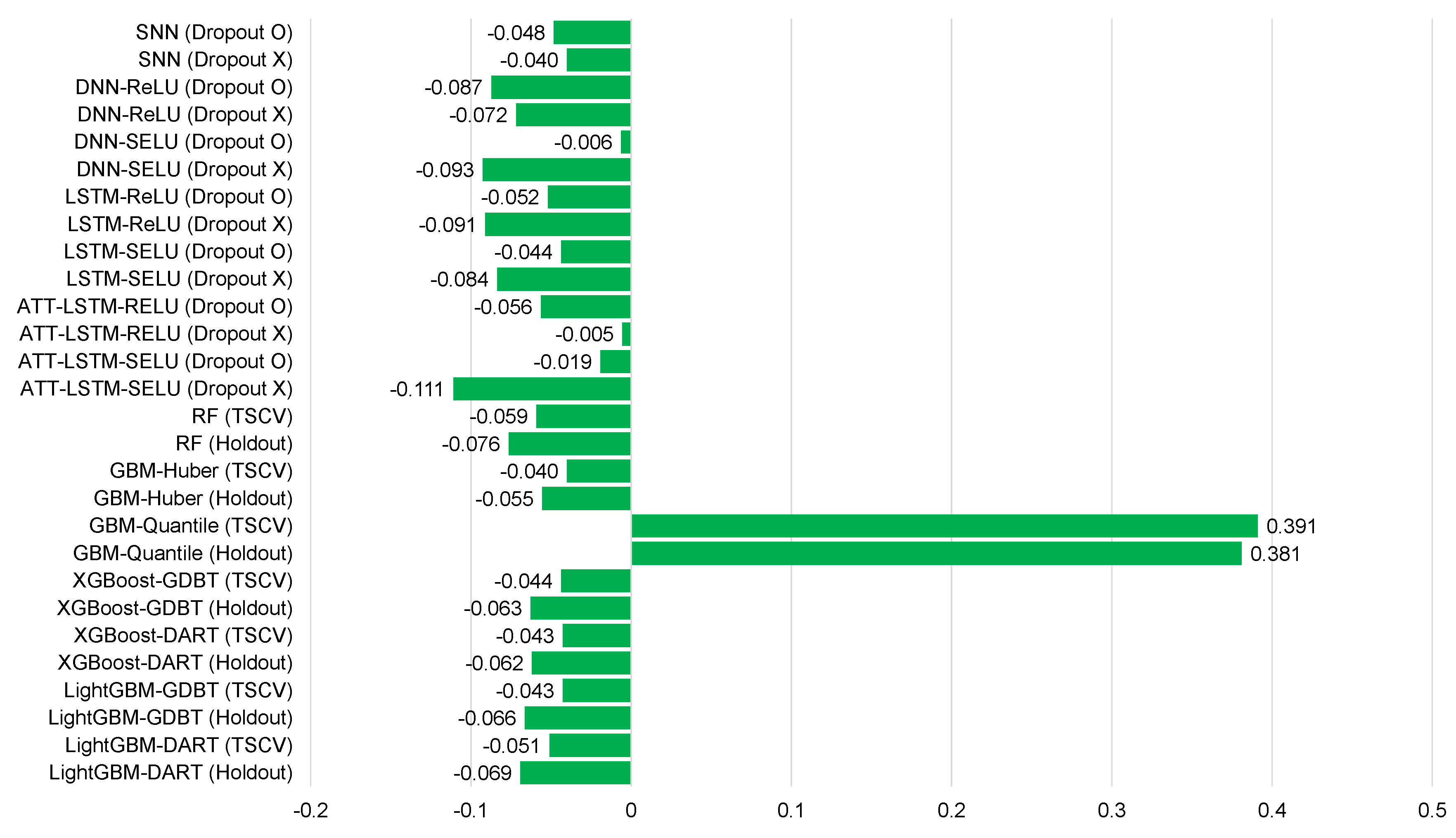
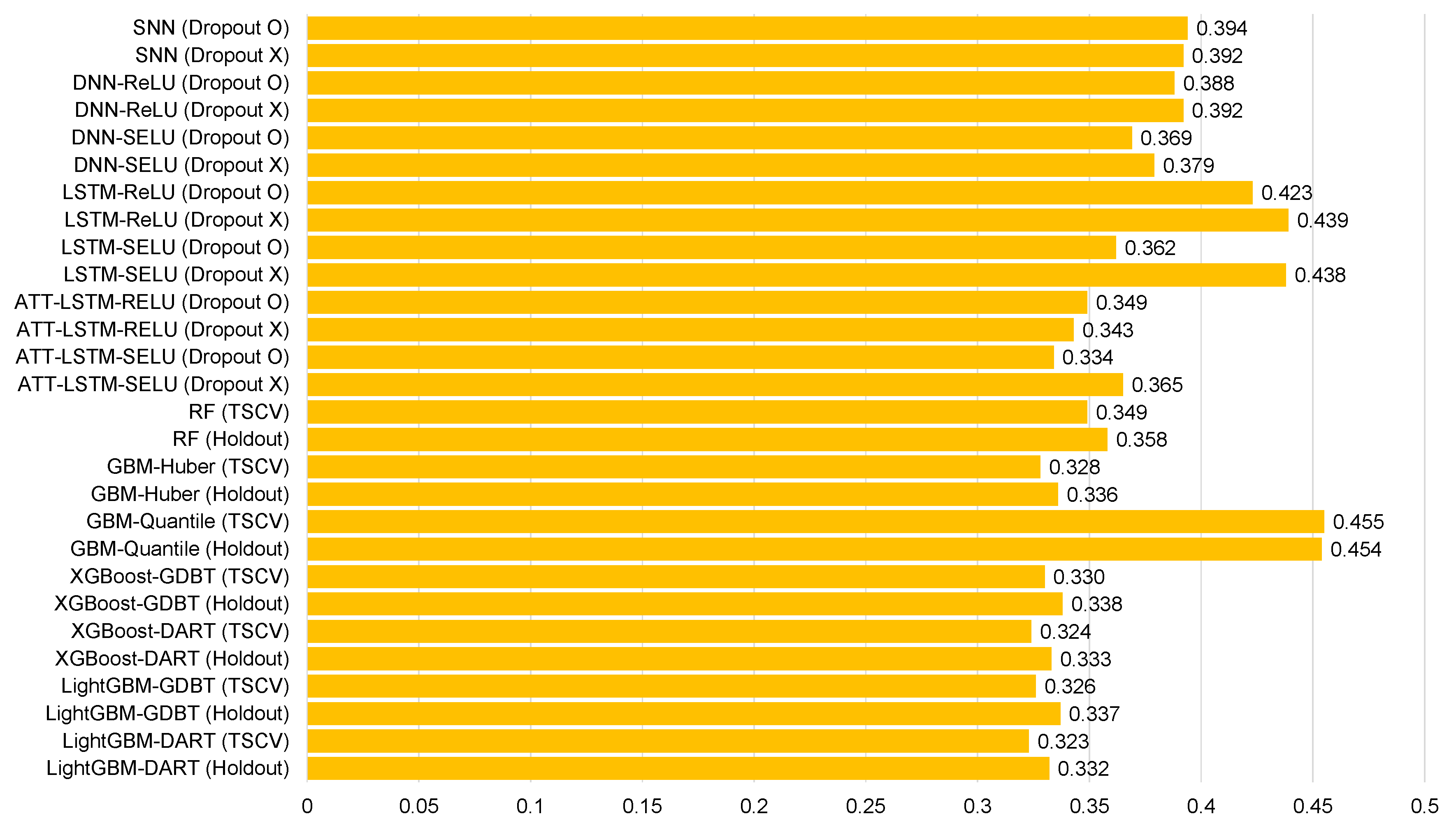
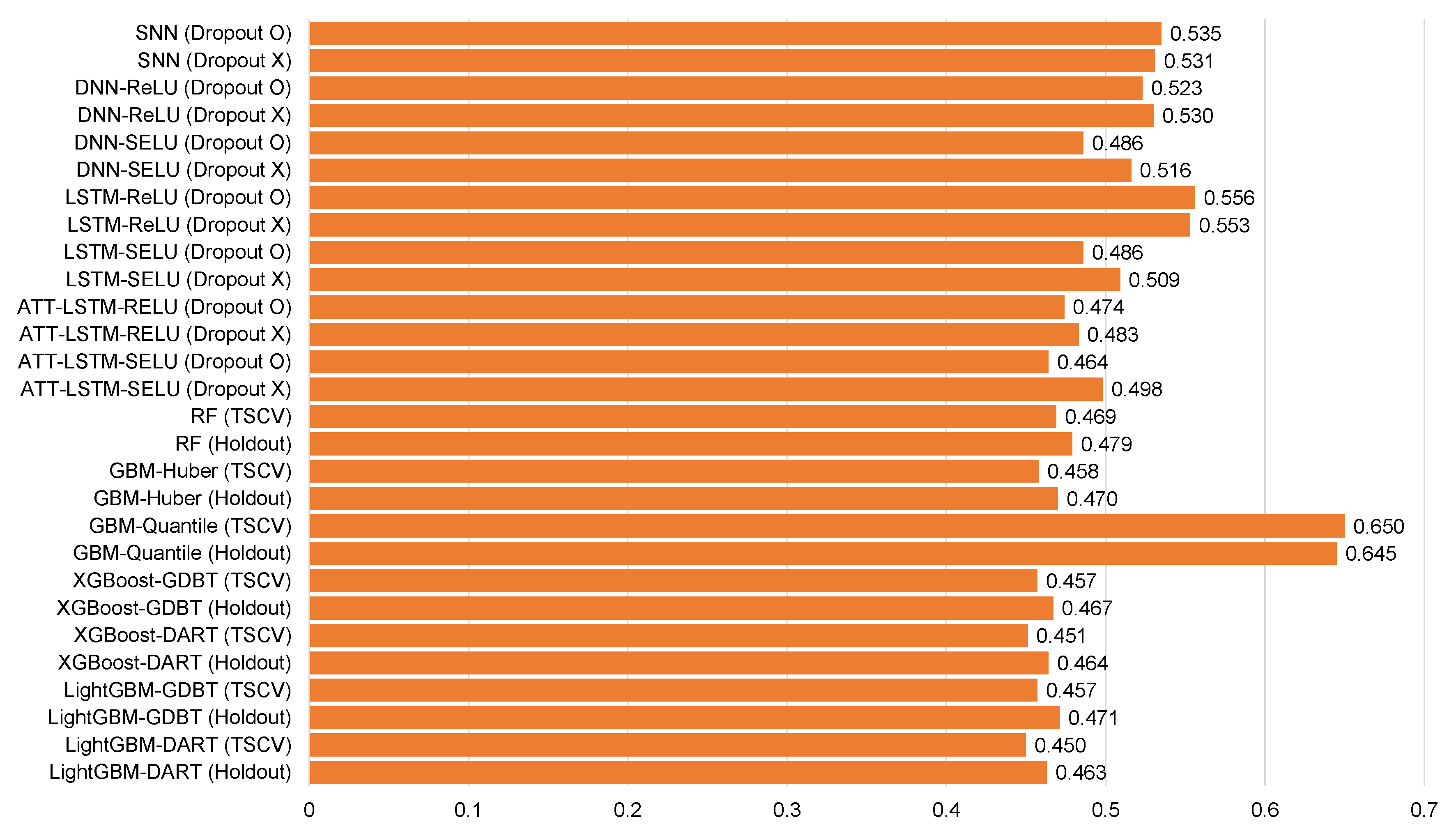
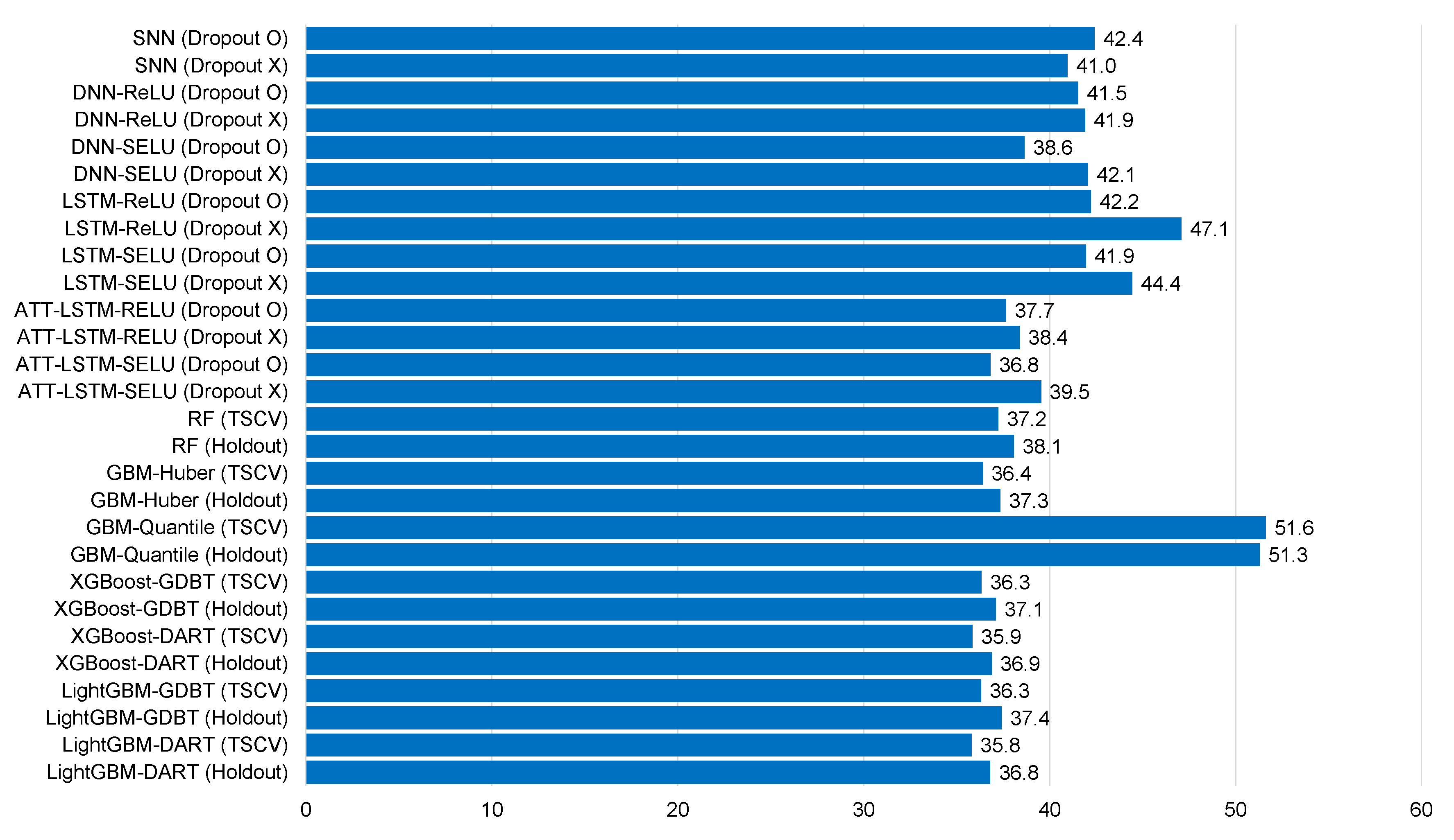
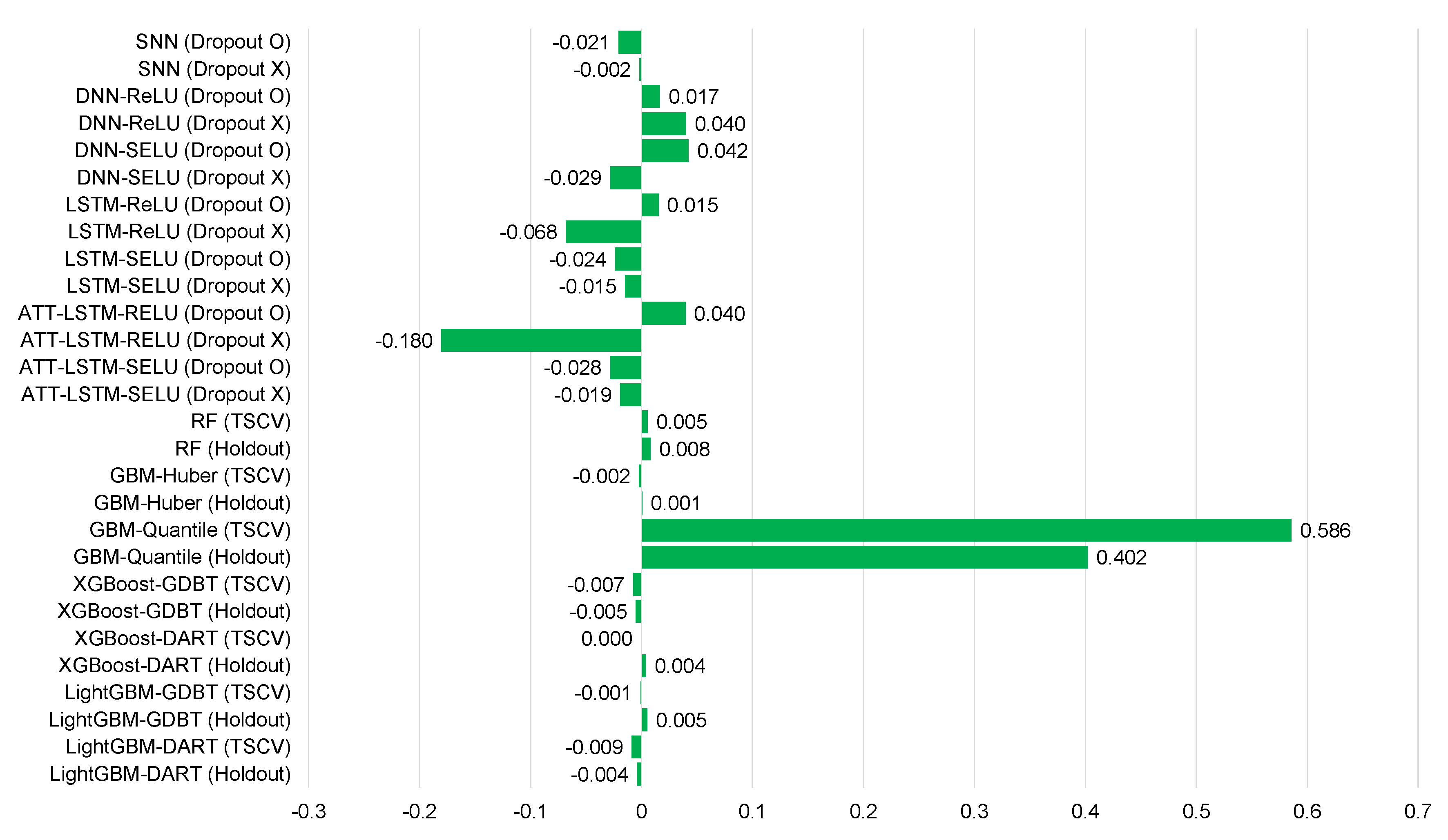
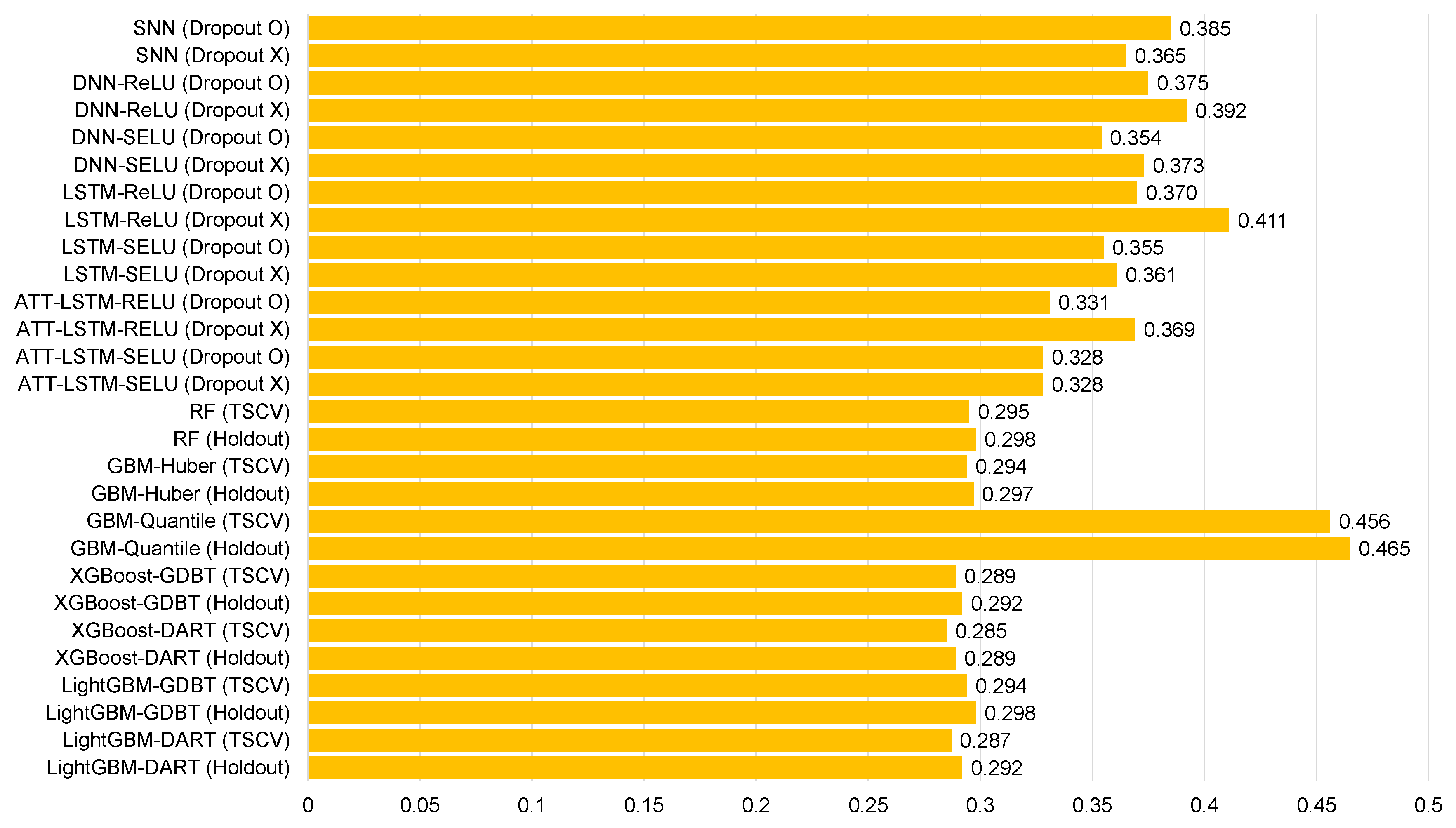
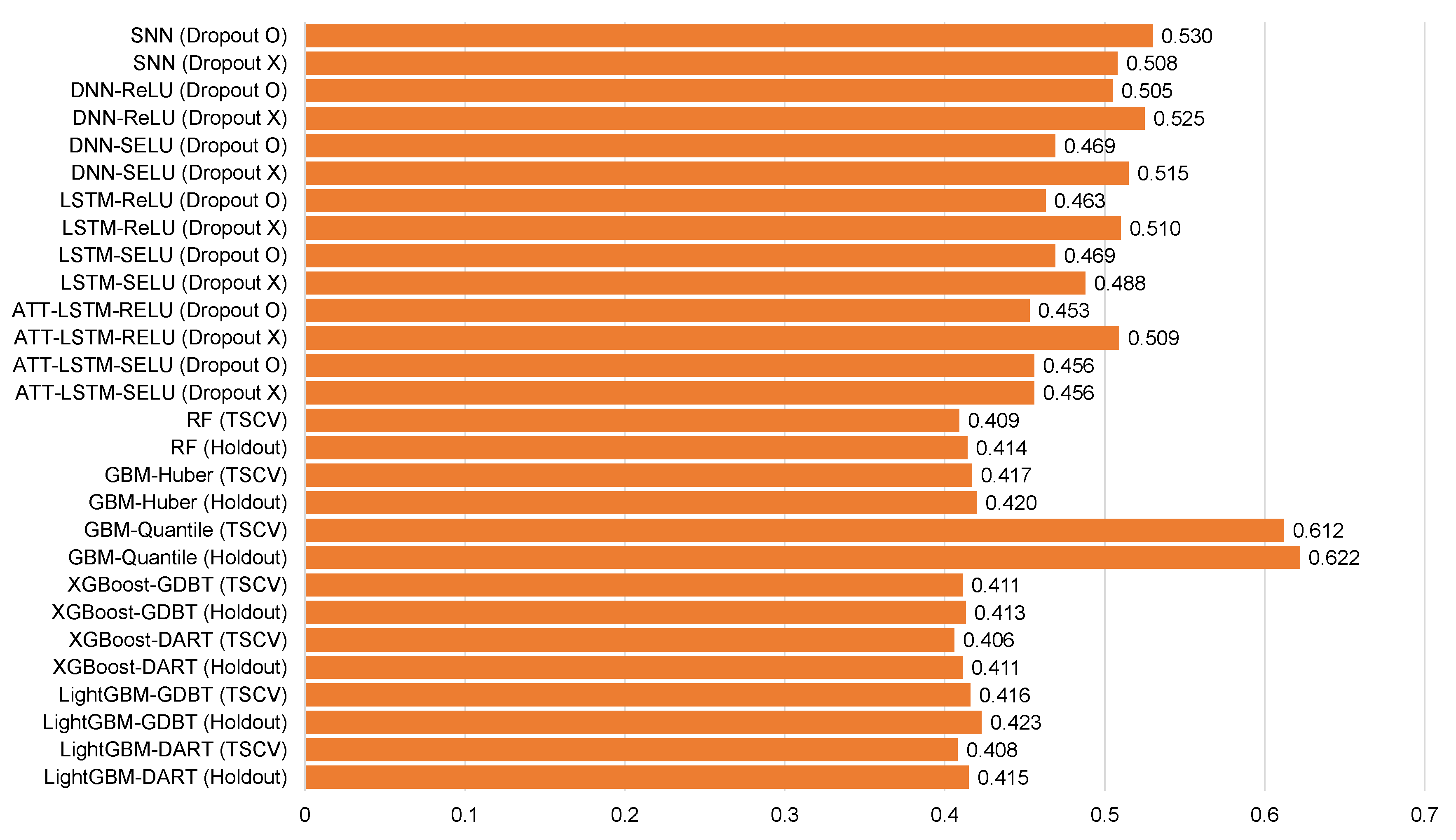
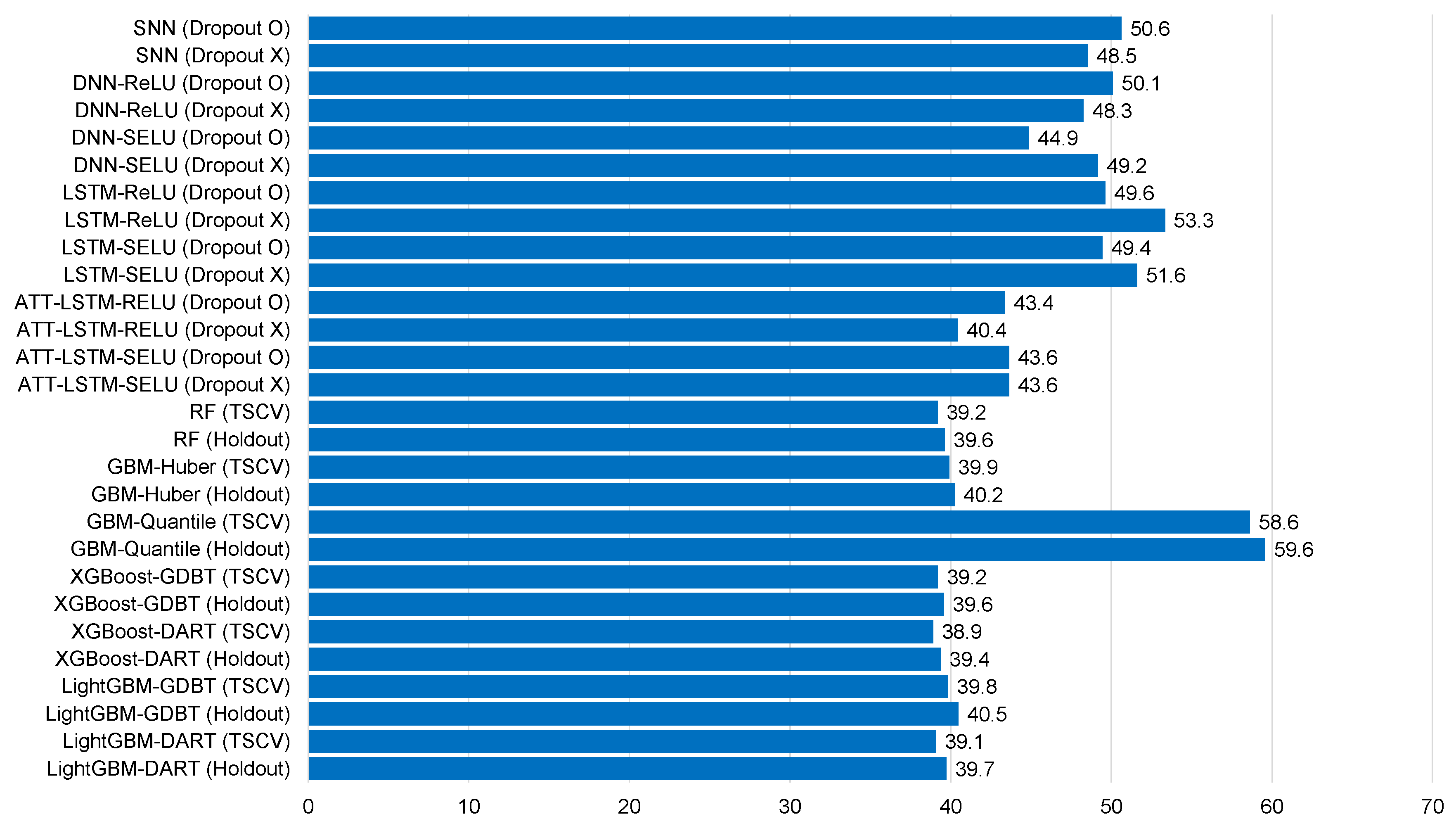
Models	Ildo-1				Gosan-ri
	MBE	MAE	RMSE	NRMSE	MBE	MAE	RMSE	NRMSE
SNN (Dropout O)	−0.048	0.394	0.535	42.4	−0.021	0.530	0.385	50.6
SNN (Dropout X)	−0.040	0.392	0.531	41.0	−0.002	0.508	0.365	48.5
DNN-ReLU (Dropout O)	−0.087	0.388	0.523	41.5	0.017	0.505	0.375	50.1
DNN-ReLU (Dropout X)	−0.072	0.392	0.530	41.9	0.040	0.525	0.392	48.3
DNN-SELU (Dropout O)	−0.006	0.369	0.486	38.6	0.042	0.469	0.354	44.9
DNN-SELU (Dropout X)	−0.093	0.379	0.516	42.1	−0.029	0.515	0.373	49.2
LSTM-ReLU (Dropout O)	−0.052	0.423	0.556	42.2	0.015	0.463	0.370	49.6
LSTM-ReLU (Dropout X)	−0.091	0.439	0.553	47.1	−0.068	0.510	0.411	53.3
LSTM-SELU (Dropout O)	−0.044	0.362	0.486	41.9	−0.024	0.469	0.355	49.4
LSTM-SELU (Dropout X)	−0.084	0.438	0.509	44.4	−0.015	0.488	0.361	51.6
ATT-LSTM-RELU (Dropout O)	−0.056	0.349	0.474	37.7	0.040	0.453	0.331	43.4
ATT-LSTM-RELU (Dropout X)	−0.005	0.343	0.483	38.4	−0.180	0.509	0.369	40.4
ATT-LSTM-SELU (Dropout O)	−0.019	0.334	0.464	36.8	−0.028	0.456	0.328	43.6
ATT-LSTM-SELU (Dropout X)	−0.111	0.365	0.498	39.5	−0.019	0.456	0.328	43.6
RF (TSCV)	−0.059	0.349	0.469	37.2	0.005	0.409	0.295	39.2
RF (Holdout)	−0.076	0.358	0.479	38.1	0.008	0.414	0.298	39.6
GBM-Huber (TSCV)	−0.040	0.328	0.458	36.4	−0.002	0.417	0.294	39.9
GBM-Huber (Holdout)	−0.055	0.336	0.470	37.3	0.001	0.420	0.297	40.2
GBM-Quantile (TSCV)	0.391	0.455	0.650	51.6	0.586	0.612	0.456	58.6
GBM-Quantile (Holdout)	0.381	0.454	0.645	51.3	0.402	0.622	0.465	59.6
XGBoost-GDBT (TSCV)	−0.044	0.330	0.457	36.3	−0.007	0.411	0.289	39.2
XGBoost-GDBT (Holdout)	−0.063	0.338	0.467	37.1	−0.005	0.413	0.292	39.6
XGBoost-DART (TSCV)	−0.043	0.324	0.451	35.9	0.000	0.406	0.285	38.9
XGBoost-DART (Holdout)	−0.062	0.333	0.464	36.9	0.004	0.411	0.289	39.4
LightGBM-GDBT (TSCV)	−0.043	0.326	0.457	36.3	−0.001	0.416	0.294	39.8
LightGBM-GDBT (Holdout)	−0.066	0.337	0.471	37.4	0.005	0.423	0.298	40.5
LightGBM-DART (TSCV)	−0.051	0.323	0.450	35.8	−0.009	0.408	0.287	39.1
LightGBM-DART (Holdout)	−0.069	0.332	0.463	36.8	−0.004	0.415	0.292	39.7

Notes: MBE: mean bias error; MAE: mean absolute error; RMSE: root mean square error; NRMSE: normalized RMSE.

and Figure 6, Figure 7, Figure 8, Figure 9, Figure 10, Figure 11, Figure 12 and Figure 13 demonstrate that our model could achieve lower RMSE and MAE values than all other forecasting models that we considered, except the XGBoost model. In addition, tree-based ensemble models exhibited better performance than deep learning-based models. Moreover, the TSCV scheme demonstrated better prediction performance than the holdout scheme, as presented in Table 13. The XGBoost and LightGBM methods exhibited a similar prediction performance. However, regarding the aspect of the training and testing time, LightGBM took 220 s, whereas XGBoost took 3798 s. That is, LightGBM is 17 times faster than XGBoost. Hence, LightGBM has a clear advantage in terms of accuracy and time. In the forecasting results of LightGBM, we observed that the MAE and RMSE values were lowest at the first time point, and as the distance increased, these values increased.

Feature importance is a measure of variable importance when data have obtained a subset of all features. Feature importance can be determined from logistic regression or tree-based models. We determined the feature importance of our model, LightGBM-DART (TSCV), at each test point (one month) according to the TSCV cycle. Figure 14 and Figure 15 present a heat map graph that reveals the feature importance of the input variables mentioned in Table 2 for both regions. The variable importance values are exhibited in the range of 0 to 1 using minimum–maximum normalization to help readers understand. From the table, we confirmed that the day number of the year ($Dat{e}_X$ and $Dat{e}_y$) consistently exhibited high feature importance, and the temperature, humidity, and wind speed, among the meteorological information, presented high feature importance. In particular, the importance of humidity increased over time.

4. Conclusions

In this paper, we proposed an MSA global solar radiation forecasting method based on LightGBM. To do this, we first configured 330 input variables considering the time and weather information provided by KMA to forecast the global solar radiation at multiple time points over the next 24 h. Then, we constructed a LightGBM-based forecasting model with DART boosting. To evaluate the performance of our model, we implemented diverse ensemble-based models and deep learning-based models and compared their performance using global solar radiation data from Jeju Island. From the comparison, we confirmed that our model exhibited better forecasting performance than other methods. We plan to conduct a forecasting model using only historical global solar radiation data in the future to provide accurate global solar radiation forecasting in regions where meteorological information is not provided. We will also conduct smart grid scheduling based on photovoltaic forecasting.

References

- Moon, J.; Kim, K.-H.; Kim, Y.; Hwang, E. A Short-Term Electric Load Forecasting Scheme Using 2-Stage Predictive Analytics. In Proceedings of the IEEE International Conference on Big Data and Smart Computing (BigComp), Shanghai, China, 15–17 January 2018; pp. 219–226. [Google Scholar] [CrossRef]
- Abdel-Nasser, M.; Mahmoud, K. Accurate photovoltaic power forecasting models using deep LSTM-RNN. Neural Comput. Appl. 2019, 31, 2727–2740. [Google Scholar] [CrossRef]
- Son, M.; Moon, J.; Jung, S.; Hwang, E. A Short-Term Load Forecasting Scheme Based on Auto-Encoder and Random Forest. In Proceedings of the International Conference on Applied Physics, System Science and Computers, Dubrovnik, Croatia, 26–28 September 2018; pp. 138–144. [Google Scholar] [CrossRef]
- Moon, J.; Park, J.; Hwang, E.; Jun, S. Forecasting power consumption for higher educational institutions based on machine learning. J. Supercomput. 2018, 74, 3778–3800. [Google Scholar] [CrossRef]
- Wang, H.Z.; Li, G.Q.; Wang, G.B.; Peng, J.C.; Jiang, H.; Liu, Y.T. Deep learning based ensemble approach for probabilistic wind power forecasting. Appl. Energy 2017, 188, 56–70. [Google Scholar] [CrossRef]
- Moon, J.; Kim, Y.; Son, M.; Hwang, E. Hybrid Short-Term Load Forecasting Scheme Using Random Forest and Multilayer Perceptron. Energies 2018, 11, 3283. [Google Scholar] [CrossRef]
- Jung, S.; Moon, J.; Park, S.; Hwang, E. A Probabilistic Short-Term Solar Radiation Prediction Scheme Based on Attention Mechanism for Smart Island. KIISE Trans. Comput. Pract. 2019, 25, 602–609. [Google Scholar] [CrossRef]
- Park, S.; Moon, J.; Jung, S.; Rho, S.; Baik, S.W.; Hwang, E. A Two-Stage Industrial Load Forecasting Scheme for Day-Ahead Combined Cooling, Heating and Power Scheduling. Energies 2020, 13, 443. [Google Scholar] [CrossRef]
- Lee, M.; Lee, W.; Jung, J. 24-Hour photovoltaic generation forecasting using combined very-short-term and short-term multivariate time series model. In Proceedings of the 2017 IEEE Power & Energy Society General Meeting, Chicago, IL, USA, 16–20 July 2017; pp. 1–5. [Google Scholar] [CrossRef]
- Khosravi, A.; Koury, R.N.N.; Machado, L.; Pabon, J.J.G. Prediction of hourly solar radiation in Abu Musa Island using machine learning algorithms. J. Clean. Prod. 2018, 176, 63–75. [Google Scholar] [CrossRef]
- Meenal, R.; Selvakumar, A.I. Assessment of SVM, empirical and ANN based solar radiation prediction models with most influencing input parameters. Renew. Energy 2018, 121, 324–343. [Google Scholar] [CrossRef]
- Aggarwal, S.; Saini, L. Solar energy prediction using linear and non-linear regularization models: A study on AMS (American Meteorological Society) 2013–14 Solar Energy Prediction Contest. Energy 2014, 78, 247–256. [Google Scholar] [CrossRef]
- Yadav, A.K.; Chandel, S. Solar radiation prediction using Artificial Neural Network techniques: A review. Renew. Sustain. Energy Rev. 2014, 33, 772–781. [Google Scholar] [CrossRef]
- Rao, K.D.V.S.K.; Premalatha, M.; Naveen, C. Analysis of different combinations of meteorological parameters in predicting the horizontal global solar radiation with ANN approach: A case study. Renew. Sustain. Energy Rev. 2018, 91, 248–258. [Google Scholar] [CrossRef]
- Cornaro, C.; Pierro, M.; Bucci, F. Master optimization process based on neural networks ensemble for 24-h solar irradiance forecast. Sol. Energy 2015, 111, 297–312. [Google Scholar] [CrossRef]
- Dahmani, K.; Dizene, R.; Notton, G.; Paoli, C.; Voyant, C.; Nivet, M.L. Estimation of 5-min time-step data of tilted solar global irradiation using ANN (Artificial Neural Network) model. Energy 2014, 70, 374–381. [Google Scholar] [CrossRef]
- Leva, S.; Dolara, A.; Grimaccia, F.; Mussetta, M.; Sahin, E. Analysis and validation of 24 hours ahead neural network forecasting for photovoltaic output power. Math. Comput. Simul. 2017, 131, 88–100. [Google Scholar] [CrossRef]
- Amrouche, B.; le Pivert, X. Artificial neural network based daily local forecasting for global solar radiation. Appl. Energy 2014, 130, 333–341. [Google Scholar] [CrossRef]
- Kaba, K.; Sarıgül, M.; Avcı, M.; Kandırmaz, H.M. Estimation of daily global solar radiation using deep learning model. Energy 2018, 162, 126–135. [Google Scholar] [CrossRef]
- Qing, X.; Niu, Y. Hourly day-ahead solar irradiance prediction using weather forecasts by LSTM. Energy 2018, 148, 461–468. [Google Scholar] [CrossRef]
- Benali, L.; Notton, G.; Fouilloy, A.; Voyant, C.; Dizene, R. Solar radiation forecasting using artificial neural network and random forest methods: Application to normal beam, horizontal diffuse and global components. Renew. Energy 2019, 132, 871–884. [Google Scholar] [CrossRef]
- Lee, J.; Wang, W.; Harrou, F.; Sun, Y. Reliable solar irradiance prediction using ensemble learning-based models: A comparative study. Energy Conv. Manag. 2020, 208, 112582. [Google Scholar] [CrossRef]
- Rew, J.; Cho, Y.; Moon, J.; Hwang, E. Habitat Suitability Estimation Using a Two-Stage Ensemble Approach. Remote Sens. 2020, 12, 1475. [Google Scholar] [CrossRef]
- Kim, J.; Moon, J.; Hwang, E.; Kang, P. Recurrent inception convolution neural network for multi short-term load forecasting. Energy Build. 2019, 194, 328–341. [Google Scholar] [CrossRef]
- Jung, S.; Moon, J.; Park, S.; Rho, S.; Baik, S.W.; Hwang, E. Bagging Ensemble of Multilayer Perceptrons for Missing Electricity Consumption Data Imputation. Sensors 2020, 20, 1772. [Google Scholar] [CrossRef]
- Kim, K.H.; Oh, J.K.-W.; Jeong, W. Study on Solar Radiation Models in South Korea for Improving Office Building Energy Performance Analysis. Sustainability 2016, 8, 589. [Google Scholar] [CrossRef]
- Lee, M.; Park, J.; Na, S.-I.; Choi, H.S.; Bu, B.-S.; Kim, J. An Analysis of Battery Degradation in the Integrated Energy Storage System with Solar Photovoltaic Generation. Electronics 2020, 9, 701. [Google Scholar] [CrossRef]
- Ke, G.; Meng, Q.; Finley, T.; Wang, T.; Chen, W.; Ma, W.; Ye, Q.; Liu, T. LightGBM: A highly efficient gradient boosting decision tree. In Advances in Neural Information Processing Systems; Morgan Kaufmann Publishers: San Mateo, CA, USA, 2017; pp. 3148–3156. [Google Scholar]
- Rashmi, K.V.; Gilad-Bachrach, R. DART: Dropouts meet Multiple Additive Regression Trees. In Proceedings of the AISTATS, San Diego, CA, USA, 9–12 May 2015. [Google Scholar]
- De Livera, A.M.; Hyndman, R.J.; Snyder, R.D. Forecasting time series with complex seasonal patterns using exponential smoothing. J. Am. Stat. Assoc. 2011, 106, 1513–1527. [Google Scholar] [CrossRef]
- Breiman, L.E.O. Random Forests. Mach. Learn. 2001, 45, 5–32. [Google Scholar] [CrossRef]
- Natekin, A.; Knoll, A. Gradient Boosting Machines: A Tutorial. Front. Neurorobot. 2013, 7, 21. [Google Scholar] [CrossRef]
- Chen, T.; Guestrin, C. XGBoost: A scalable tree boosting system. In Proceedings of the 22nd ACM SIGKDD International Conference on Knowledge Discovery and Data Mining, San Francisco, CA, USA, 13–17 August 2016. [Google Scholar]
- Park, S.; Moon, J.; Hwang, E. 2-Stage Electric Load Forecasting Scheme for Day-Ahead CCHP Scheduling. In Proceedings of the IEEE International Conference on Power Electronics and Drive System (PEDS), Toulouse, France, 9–12 July 2019. [Google Scholar] [CrossRef]
- Rahman, R.; Otridge, J.; Pal, R. IntegratedMRF: Random forest-based framework for integrating prediction from different data types. Bioinformatics 2017, 33, 1407–1410. [Google Scholar] [CrossRef] [PubMed]
- Pedregosa, F.; Varoquaux, G.; Gramfort, A.; Michel, V.; Thirion, B.; Grisel, O.; Blondel, M.; Prettenhofer, P.; Weiss, R.; Dubourg, V. Scikit-learn: Machine learning in Python. J. Mach. Learn. Res. 2011, 12, 2825–2830. [Google Scholar]
- Feng, C.; Cui, M.; Hodge, B.-M.; Zhang, J. A data-driven multi-model methodology with deep feature selection for short-term wind forecasting. Appl. Energy 2017, 190, 1245–1257. [Google Scholar] [CrossRef]
- Moon, J.; Park, S.; Rho, S.; Hwang, E. A comparative analysis of artificial neural network architectures for building energy consumption forecasting. Int. J. Distrib. Sens. Netw. 2019, 15. [Google Scholar] [CrossRef]
- Moon, J.; Jung, S.; Rew, J.; Rho, S.; Hwang, E. Combination of short-term load forecasting models based on a stacking ensemble approach. Energy Build. 2020, 216, 109921. [Google Scholar] [CrossRef]
- Hochreiter, S.; Schmidhuber, J. Long short-term memory. Neural Comput. 1997, 9, 1735–1780. [Google Scholar] [CrossRef]
- Bahdanau, D.; Cho, K.; Bengio, Y. Neural machine translation by jointly learning to align and translate. In Proceedings of the International Conference on Learning Representations, San Diego, CA, USA, 7–9 May 2015. [Google Scholar]
- Li, H.; Shen, Y.; Zhu, Y. Stock Price Prediction Using Attention-based Multi-Input LSTM. In Proceedings of the 10th Asian Conference on Machine Learning (ACML 2018), Beijing, China, 14–16 November 2018; pp. 454–469. [Google Scholar]
- Klambauer, G.; Unterthiner, T.; Mayr, A.; Hochreiter, S. Self-Normalizing Neural Networks. In Proceedings of the 31st International Conference on Neural Information Processing Systems (NIPS 2017), Long Beach, CA, USA, 4–9 December 2017; pp. 971–980. [Google Scholar]
- Moon, J.; Kim, J.; Kang, P.; Hwang, E. Solving the Cold-Start Problem in Short-Term Load Forecasting Using Tree-Based Methods. Energies 2020, 13, 886. [Google Scholar] [CrossRef]