Automated Extraction of Visible Floodwater in Dense Urban Areas from RGB Aerial Photos

Abstract

Rapid response mapping of floodwater extents in urbanized areas, while essential for early damage assessment and rescue operations, also presents significant image interpretation challenges. Images from visible band (red–green–blue (RGB)) remote sensors are the most common and cost-effective for real-time applications. Based on an understanding of the differing characteristics of turbid floodwater and urban land surface classes, a robust method was developed and automatized to extract visible floodwater using RGB band digital numbers. The methodology was applied to delineate visible floodwater distribution from very high-resolution aerial image data acquired during the 2013 Calgary flood event. The methodology development involved segment- and pixel-based feature analysis, rule development, automated feature extraction, and result validation processing. The accuracies for the visible floodwater class were above 0.8394% and the overall accuracies were above 0.9668% at both pixel and segment levels for three test sites with diverse urban landscapes.

1. Introduction

The combination of rapid urbanization and climate change resulted in increased occurrence of major urban flood events across the globe, especially for those cities located along coastal lines and in floodplains of major rivers [1,2]. Urban floods present high risk to dense resident populations, as well as to valuable and complex infrastructure [3]. Timeliness is a critical requirement for the provision of information during flood disasters in urban areas. Real-time geographic extents of flooded areas delineated using remote sensing data and technologies represent one of the key information inputs for effective disaster management and rapid rescue response [4].

Flooding in urban areas can be grouped into three categories. These include inundation in coastal areas due to rising sea levels caused by tsunamis, tropical storms, and the effects of climate change (type A, also referred to as “coastal flood”). Inland cities, on the other hand, are susceptible to flooding from severe local rain events or river surges due to heavy upstream precipitation or snow melt (type B, also referred to as “fluvial flood”). In the case of local storm events, run-off water management can be greatly impacted by aspects of the urban landscape. For example, high levels of impervious cover, usually associated with high-intensity urbanization, result in greater run-off volumes and shorter run-off response time, thereby putting great stress on storm sewer infrastructure (type C, also referred to as “pluvial flood” or “flash flood”). The data inputs and information extraction methodologies needed for rapid disaster response or pre-event preparation vary depending on the urban flood type. Remote sensing data and techniques were identified as being useful for providing real-time estimates of floodwater distribution and flood area change in the case of type A and B disasters in rural and open land areas [5]. Delineation of floodwater distribution in dense urban areas using remotely sensed imagery presents additional challenges due to the complexity of urban landscapes and morphologies [6].

For operational visible flood mapping in disaster emergency response, satellite synthetic aperture radar (SAR) image data are widely used [7,8,9,10,11,12,13], since SAR imagery can be acquired under all weather conditions. On the other hand, SAR imagery of urban areas is difficult to interpret because of complexities arising from the off-nadir viewing configuration of such sensors. These complexities can include (a) confusion of floodwaters with specular reflection of smooth land surfaces such as pavement, (b) extensive ground areas that are not imaged because of shadowing, and (c) overlay effects that merge reflections from physically separated areas into the same sensor resolution cell [6]. Recently, progress from tests using InSAR (interferometric synthetic aperture radar) coherence for floodwater mapping in urban areas was reported [14,15]. Optical remote sensing imagery data with low to medium spatial resolution (e.g., those from Landsat TM and MSS, MODIS) are used broadly for regional flood mapping and monitoring [16,17]. These sensors, which include near- and medium-infrared spectral bands, as well as visible bands (hereafter referred to as red–green–blue (RGB) bands), have a cost-effective advantage over SAR data for operational flood extent mapping, under cloud-free conditions. Furthermore, many floodwater products were generated from a combination of active and passive image data for the creation of long-term flood records (e.g., Reference [18]). Optical imagery was used as an information source for water surface detection, as well as for a broad range of water quality issues (see Reference [19] for an excellent review of the state of the art in this research field). Indices, derived from arithmetic combinations of spectral bands, were evaluated to map waterbodies with a range of quality measures including dissolved organic matter, chlorophyll a, and total suspended solids. However, these indices, including the normalized difference water index (NDWI) [20], the modified NDWI [21], the automated water extraction index [22], and the water ratio index [23], which can be used for water surface detection, require both visible and infrared bands. Some spectral indices targeted at water quality assessments were proposed that involve ratios of visible band responses, which were used to map total suspended solids and turbidity using Landsat imagery (e.g., Reference [24,25]). Mapping of urban turbid floodwater, which is usually in fragment patterns, on the other hand, requires higher-resolution coverage and must deal with fast-flowing water, as well as placid water conditions.

For real-time mapping of floodwater distribution, airborne imagery (including data from sensors mounted on both aircraft and unmanned aerial vehicles (UAVs)) has advantages over satellite optical data since its spatial resolution is typically higher [26], acquisition times can be flexible to provide data during critical times of the flood event, and acquisitions can be made from under cloud layers if necessary. Historically, aircraft are the primary sensor platform for acquisition. The design and performance of UAVs for civil applications do not yet, in most events, meet the requirements for disaster mapping over large areas. In the future, low-cost, high-endurance UAVs are anticipated to play a key role in the disaster monitoring. Feng et al. [27] used high-resolution imagery from UAV with long power endurance (1.5 hour) for floodwater mapping over an urban area with coverage of 10 km². A random forest classifier using RGB spectral and texture information was used for floodwater mapping, although the rules used in the classifier were not presented explicitly in the public scientific literature to facilitate further use by others.

The optical image sources discussed above can only provide direct estimates of “visible” flooded areas, i.e., those areas with unobstructed lines of sight to the parent sensor. In urban areas, since the landscapes and infrastructure morphologies in dense urban areas are diversified and complex, the floodwater extent that is visible to the sensor appears spatially fragmented, as some ground level areas are obscured by, for example, tree canopies and, in the case of off-nadir imaging, tall buildings. In addition, flooded areas that are in shadow may be difficult to distinguish from dry ground because of their low reflectance levels. On the other hand, using this information on the spatial distribution of visible floodwater as a clue, hidden flooded areas can be inferred with the aid of additional information sources [28].

The most common suite of bands carried by remote sensing sensors on various Earth observation platforms (such as satellites, the International Space Station, aerial planes, and UAVs) constitutes the red–green–blue (RGB) visible bands. On the downside, RGB bands alone provide limited capability for discriminating among common land covers compared to having the addition of near-infrared and mid-infrared spectral coverage. Major challenges of real-time floodwater mapping using RGB imagery in this work are (a) timely extraction of the visible floodwater information, (b) maximizing the capability of extraction from RGB data with limited information, and (c) detection of the targets in dense urban areas with complex landscape. The objective of this work was to develop robust methodology based on RGB imagery data for rapid response mapping of the visible floodwater in dense urban areas. The developed methodology was tested in an urban flood case study. The next section of this paper describes the test sites and available datasets, including high-resolution aerial RGB imagery acquired during the Calgary 2013 flood event. This is followed by a description of the feature analysis of principal land surface classes including the target class, i.e., the visible floodwater. The feature analysis led to the development of a novel spectral index, as well as rules for the rapid extraction of visible floodwater areas. Then, the technique of targeted information extraction and a performance assessment are demonstrated using the test site data. Finally, the overall conclusions from the case study are presented.

2. Materials and Methods

The study area of this work is in the central business district and its environs of the city of Calgary, Canada, as shown in Figure 1. The city of Calgary, a major Canadian city with a population of 1.097 million (2011 census) is located at the confluence of the Bow River, flowing east–west, and the Elbow River, flowing north–south. In June 2013, the city experienced a major flooding event. Widespread heavy precipitation of more than 200 millimeters fell during the period from 19 to 21 June 2013 in the Rockies and foothills west of the city, triggering rapid rises in both the Bow and Elbow rivers [29,30]. It was a typical type B urban flood as categorized above. The impact of the disaster on populated urban areas was significant. In total, across Alberta province, 125,000 residents were affected (75,000 in Calgary alone) and costs for clean-up and damage repair exceeded five billion Canadian dollars [31].

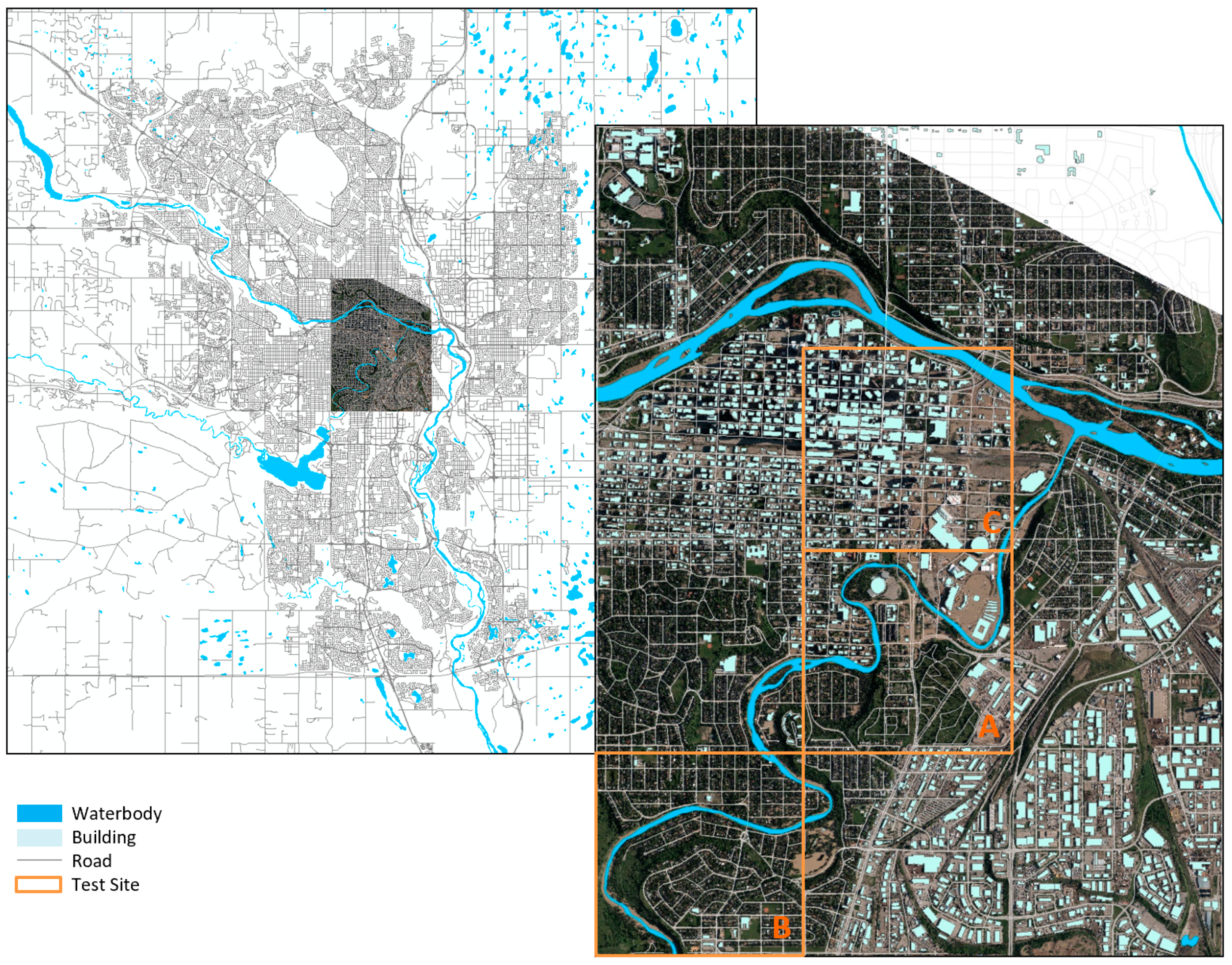
An overview of the aerial imagery is shown in Figure 1 (right). The set of true color aerial ortho-photos, taken between about 8:00 and 9:30 a.m. local time on 22 June 2013, was obtained from the city of Calgary (cityonline.calgary.ca). The cloud-free aerial photos are of three bands (RGB) with a spatial resolution of 20 cm. Since the aerial imagery was acquired after the peak time (21 June) of the flood, sediment residue was present and detectable on ground surfaces such as on the surfaces of roads and parking lots that were recently exposed following floodwater recession. In addition to the distortion of some high-rise buildings in the image due to the off-nadir imaging effects, significant shadowing was also present due to the early morning acquisition (solar elevation angle between 35 and 40 degrees).

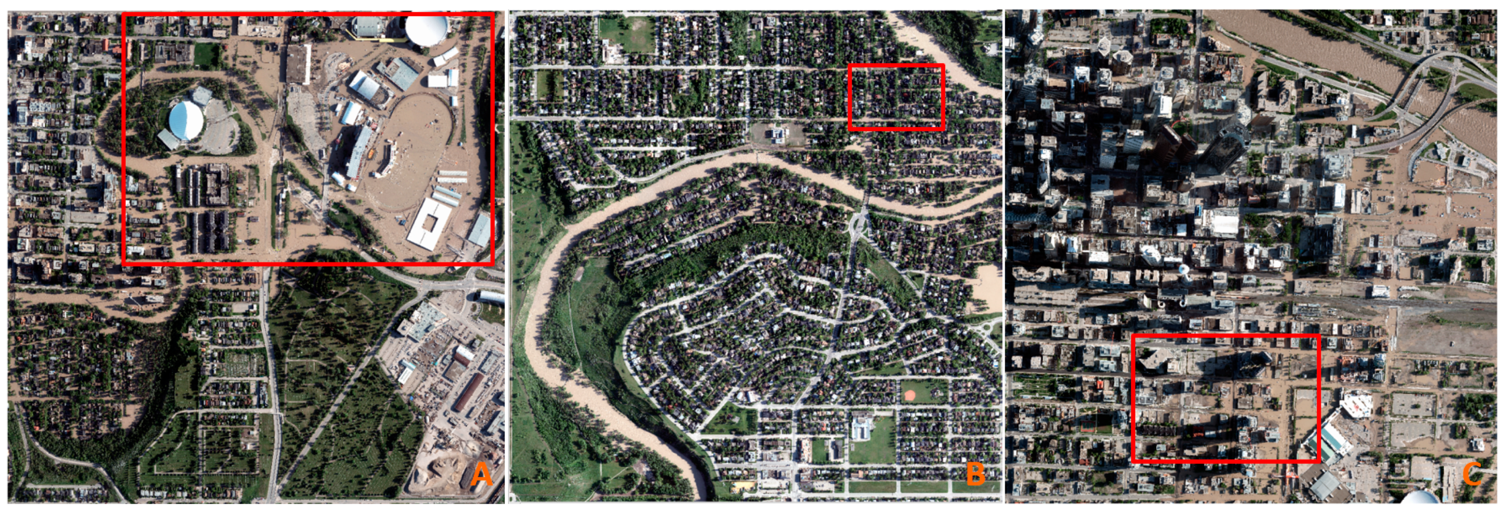
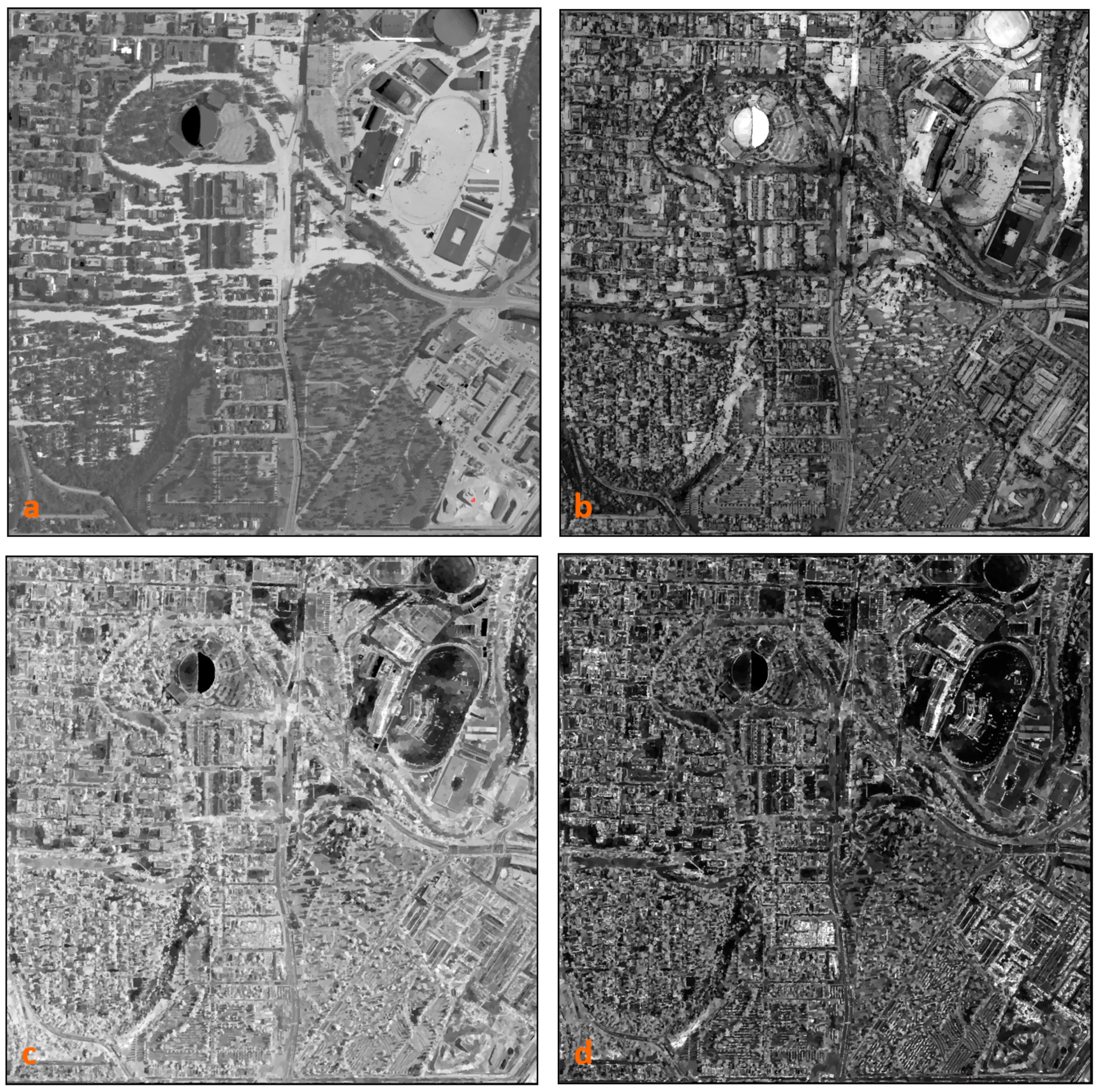
Three test sites, with a size of approximately 1.6 × 1.6 km each, were selected within the aerial photo data coverage. The coverages of these test sites are shown in Figure 1. These test sites have diverse urban land cover and land use types, as well as various complex urban landscapes (business parks, matured residential areas, and central business district). A brief description of these three sites is given in

Table 1. Description of the test sites.

Test Site	Area (km2)	Land Use	Main Landscape	Major Land Surface Features
A	2.721	Business Parks and Matured Residential Land	Low-rise buildings, single and multi-level residential buildings, public infrastructure, roads, parking lots, trees, open grass land	Building roof, road, shadow, grass, tree canopy, wet and dry soil
B	2.681	Matured Residential Land	Single residential buildings, roads, dense trees, grassy yards	Tree canopy, building roof, shadow, road
C	2.711	Central Commercial Area	Large high-rise buildings, roads and parking lots	Large building roof, road, shadow

. In addition, Figure 2 shows the aerial photo images over these test sites.

In addition to the RGB image dataset, a high-resolution digital elevation model (DEM) with a spatial resolution of 20 cm and the building footprint polygons over the Calgary center area were provided by the City of Calgary.

3. Preliminary Analysis

In order to gain insight into a possible strategy for floodwater delineation, a preliminary study was undertaken of test site A to assess the spectral properties of both water and prominent land cover types. This site was selected as it encompasses diverse land use types including residential, transportation, commercial, and light industrial. Sample areas of each key class were visually identified. Each area covered 5 × 5 pixels of pure land surface cover type. The surface cover classes selected included floodwater and shadow, as well as conventional land cover types such as grass, trees, building roofs (including large building flat roofs of various materials and residential shingle roofs), dry soil, roads, and parking lot surfaces. 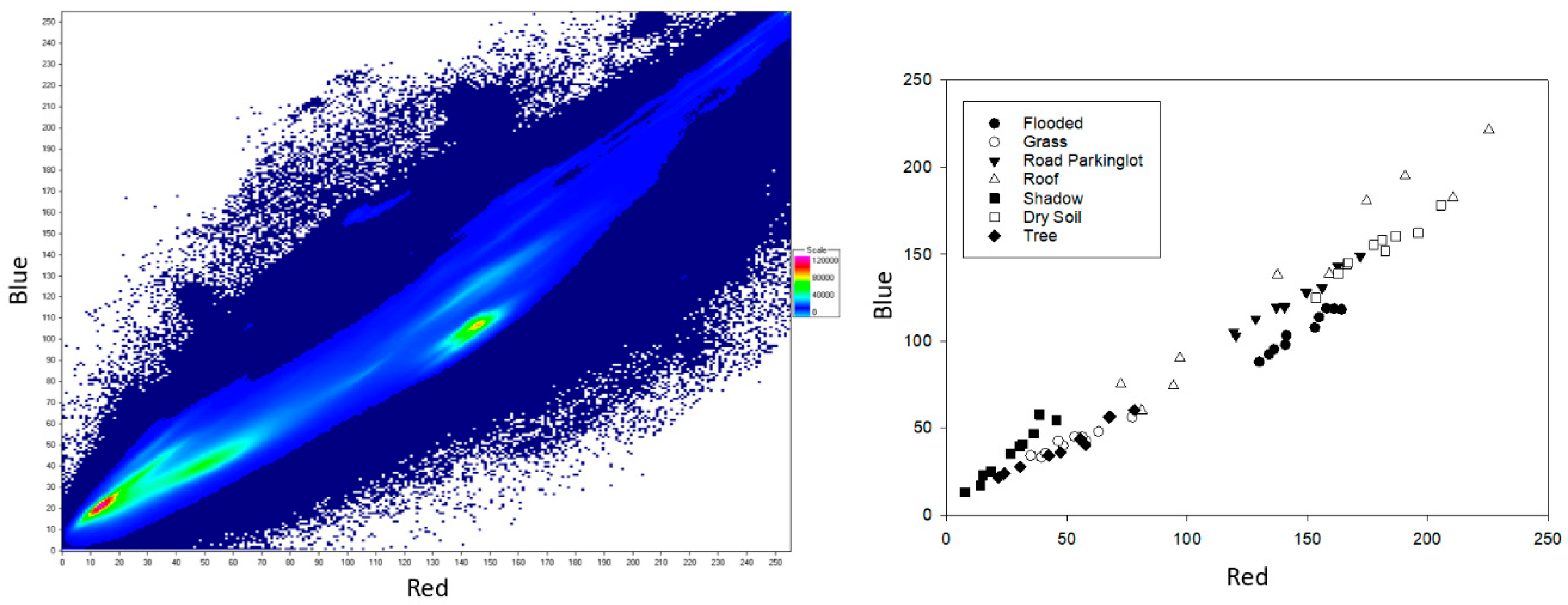Figure 3 presents a color-coded scatter plot of red vs. blue DN (digital number) values of all pixels in the image (left plot). The colors indicate pixel concentrations, where the scale of blue through green to red indicates increasing concentrations of pixels (the colored pixel number scale in Figure 3 is between 0 and 120,000 pixels). The plot on the right illustrates the locations, in the same spectral space, of reference samples of the surface classes noted above. Although the DNs of blue and red bands are highly correlated, there are clusters of samples in this space, particularly one associated with areas of floodwater (i.e., the target class). This cluster lies off the correlation line defined by land pixels. Among these land surface classes, the building rooftop class exhibited most dispersion since there was wide variation in roofing materials and roofing colors (i.e., shingles, tar, gravel, etc.). Water bodies in most scenes were clear and could be easily confused with shadow (i.e., due to low reflectance in both red and blue bands). Compared to clear water, the floodwater in our data had high reflectance in the visible bands due to its turbidity. This turbidity arose from sediment suspension (mainly soil) which increased the reflectance, particularly in the red part of the visible spectrum, while the reflectance of clear water is highest in the blue part of the spectrum. As the type of soil in the floodwater depends on the location of run-off upstream, the reflectance of the floodwater can be expected to vary depending on watershed soil types and distributions. In the Calgary flood case, the aerial photos exhibited a turbidity that appeared visually as a dark-yellow color.

The spatial characteristics of land surface features at the segment level were examined as well. The gray-level co-occurrence matrix (GLCM) and standard deviation (SD) of image segments were used to examine the similarity of floodwater with other land surface classes based on surface texture features [32]. Figure 4 shows maps of the example spatial attributes, namely, GLCM homogeneity, GLCM entropy, and SD red band, over site A. From a visual inspection of this figure, it is obvious that these texture measures did not appear to provide good segregation of visible floodwater from other land surface classes. In the complicated urban landscape like that in test site A, there was large variation in the surface textures on building roofs and other manmade surfaces (such as that of mowed grass land). In the aerial image acquired on 22 June, the surface texture of the visible floodwater varied greatly since the flow rates of floodwater varied from still to fast-flowing conditions. There were also similarities in texture between the surface of floodwater and that of other land cover classes. For example, smooth manmade surface features such as large building roofs can have similar texture feature levels to those of calm water surfaces, as shown in site A. In addition, the GLCM mean map was examined. It was found that the GLCM mean map had high similarity with the red band map (e.g., the Spearman rank order correlation between these two maps was 0.995 for test site A). The contribution of the GLCM mean was duplicated with that of the red band. Therefore, texture attributes exhibited little in the way of floodwater discrimination.

4. Methodology

From the preliminary analysis above, it was noted that visible floodwater, with a unique spectral character (i.e., higher red-band DNs), can potentially be separated from all land classes on high-resolution true color image data. To accomplish this, we propose a new information spectral index, the floodwater index (FWI), based on the differences between the DNs of the red, green, and blue bands (B_r, B_g, and B_b, respectively).

$$FWI=\frac{(B_r-B_b)+\left(B_r-B_g\right)}{100},$$

(1)

where the factor 100 is included as a simple reduction factor.

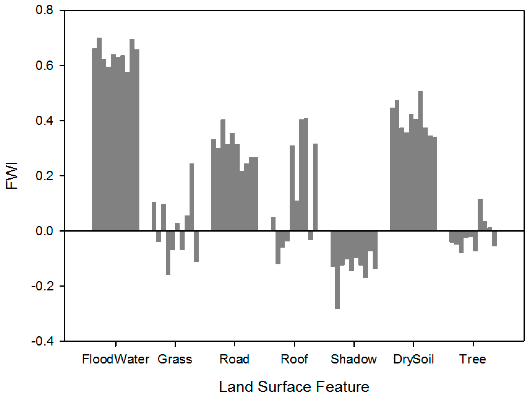
Figure 4a displays the FWI map for test site A. Further analysis involved quantifying the separability of floodwater from other land surface types based on FWI. Figure 5 illustrates the distributions of FWI values for samples of the land surface classes (including floodwater) selected from test site A. Cursory inspection of this figure suggests that the floodwater class consistently exhibited higher positive values of FWI compared to other land surface classes. While impervious surfaces and dry soil primarily exhibited positive FWI, vegetation and shadow areas exhibited negative values. To quantify floodwater separability, t-tests were undertaken comparing the FWI distributions of water versus each of the land surface class sample populations. In each case, floodwater was found to be significantly different to better than the 99.9% confidence level.

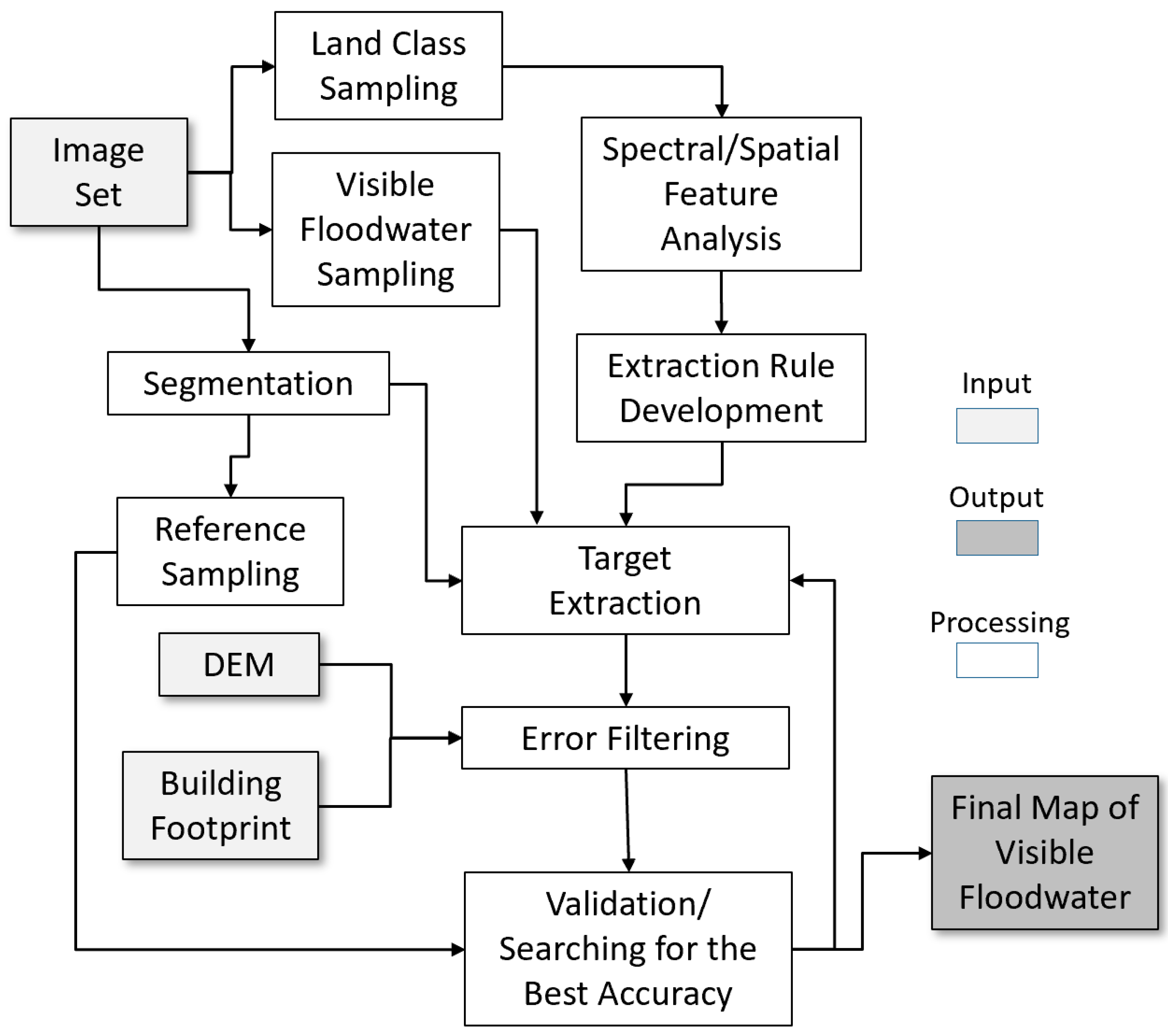
Figure 6 presents a proposed processing flow for visible floodwater delineation based on FWI. The principal steps of this approach are briefly described below.

• High-resolution image interpretation is amenable to object-based processing. As a consequence, the raw image was segmented using the eCognition package (www.ecognition.com). The values of parameters at the segment level were output from the eCognition platform for further information extraction.
• Three groups of samples were collected manually from the visual interpretation for preliminary analysis: all land surface classes (10 samples per class), those for floodwater detection (visible floodwater class, 50 samples), and those for validation, i.e., the reference sample layer with visible-floodwater and non-visible-floodwater classes (all segments for each test site, for this experimental work).
• An analysis was undertaken to assess the effectiveness of FWI in isolating floodwater from land classes in the scene, for rule development.
• For the preliminary visible floodwater mask generation, FWI and a spectral similarity comparison with visible floodwater class sample segments were employed. Application of the comparison test involved calculating the minimum RGB spectral distance (D_min) of each floodwater candidate segment (x) with each visible floodwater class sample (x_s), where

  $$D_{min}=\underset{samples}{\min }(\sqrt{{\displaystyle \sum }_{RGB}{\left(x-x_s\right)}^2}).$$

  (2)

For a segment to be classed as visible floodwater, FWI and D_min must be below designated threshold levels that are estimated by calculation for the floodwater extraction results with the best accuracies.

5.

Searching for the optimum thresholds of FWI and D_min was done to obtain the highest mean accuracy against the reference sample data for each test image tile. The mean accuracy here was the average of producer and user accuracy [33] of the visible floodwater at the segment level. A floodwater mask was generated by determining which segments could be classed as visible floodwater with a high degree of confidence linked with the best mean accuracy. Two ratio parameters, RDIS (a ratio related to D_min) and RFI (a ratio related to FWI) were used as inputs for searching the threshed to obtain optimal results with the best mean accuracy. If RDIS or RFI is R and D_min or FWI is Y, then

$$Y=Y_{min}+SD\times R,$$

(3)

where Y_min is the minimum value of Y and SD is the standard deviation of Y, with both being derived from the visible floodwater sample data.

6.

Further classification refinement was undertaken using ancillary information extracted from a DEM and building footprint databases. These information sets would typically be available in municipal databases and available for rapid response mapping. These datasets can be used for filtering some of the floodwater error pixels in the visible floodwater mask, especially those involving confusion with the building rooftops.

7.

Final accuracies were computed at the pixel and segment levels.

5. Results

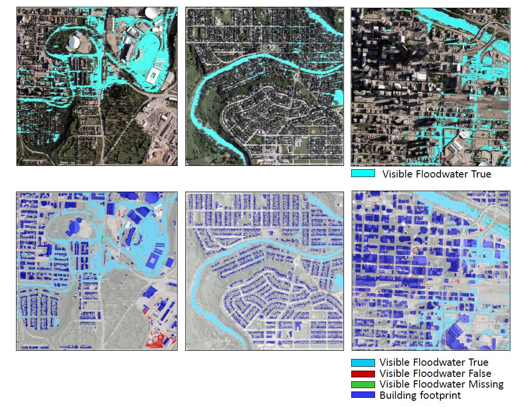
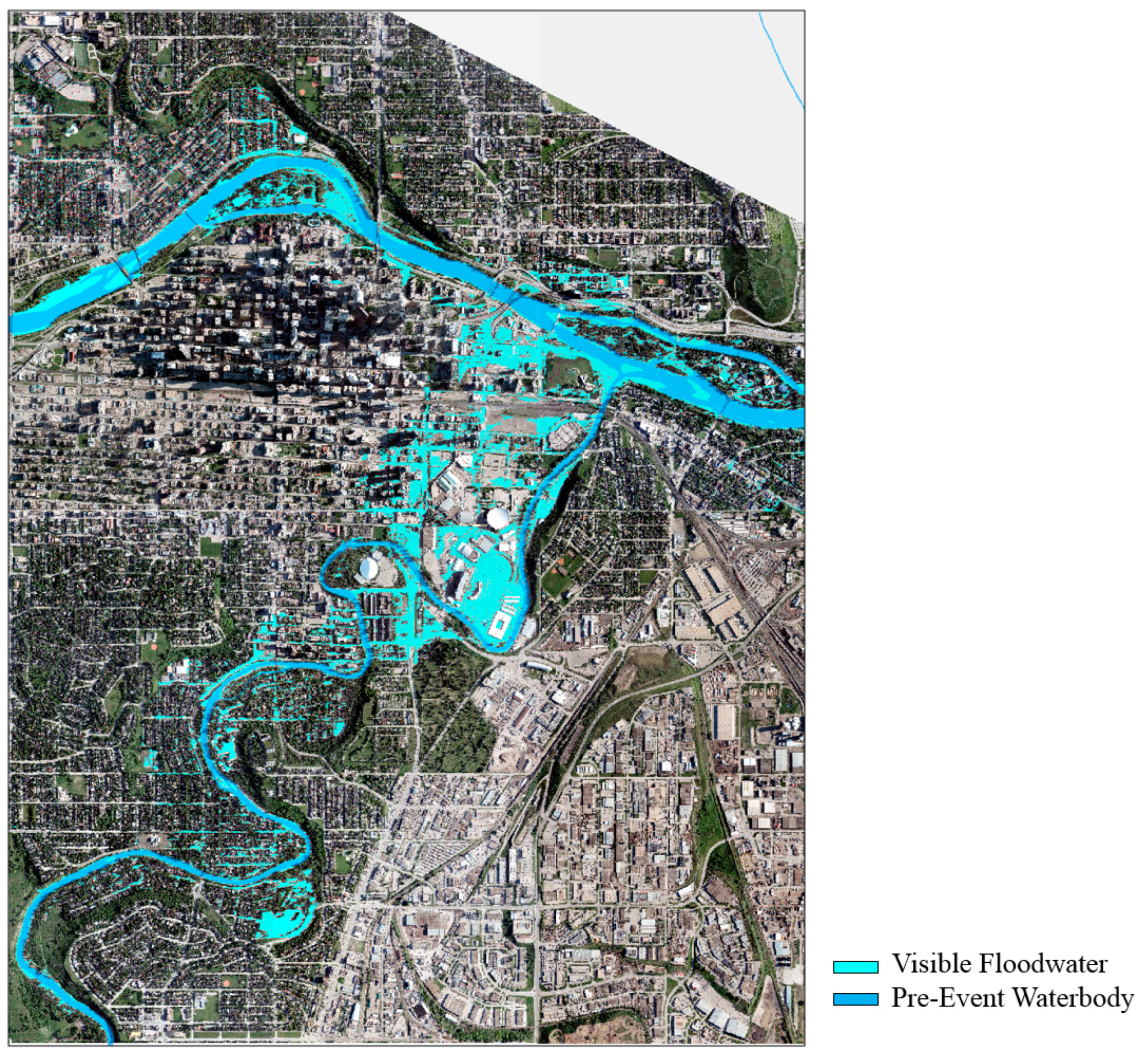
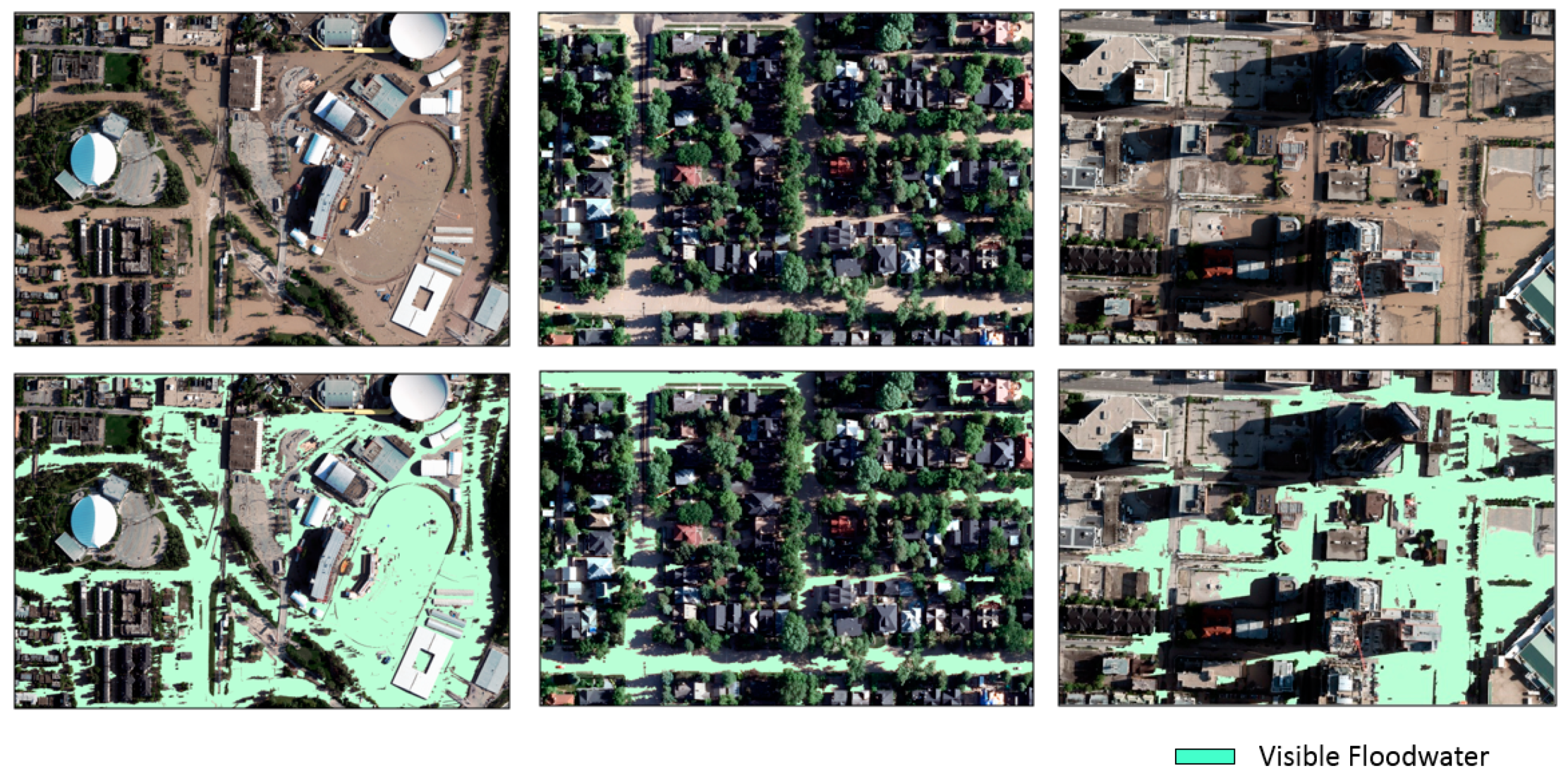
Figure 7 shows the distribution of visible floodwater extracted using the optimum FWI–spectral distance threshold combination. The coverage of the visible flooded areas was mainly over lands close to the parent river valleys including business (commercial and light industrial) districts, older residential areas, and the downtown area. The high spatial resolution of the aerial photo imagery provided good detail of the visible floodwater patterns (see the selected portions of the visible floodwater map using the zoomed-in view shown in Figure 8). It also revealed that, in high-resolution optical imagery, visible flooded areas were only a portion of the overall flooded areas in urbanized areas because of the presence of mature tree canopies and shadows cast by trees and buildings. Improvement of overall floodwater distribution mapping would require extraction of trees and accurate shadow delineation. These issues will be dealt with in a later publication.

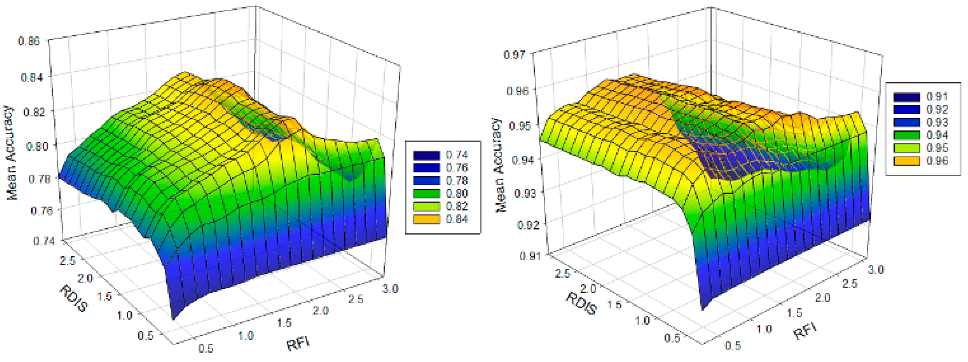
Accuracy assessment was based on two reference groups of samples, i.e., one for the target class, the visible floodwater (VFW), and the other for non-visible floodwater (NVFW), i.e., the conglomerate of land surface covers except for the visible floodwater. A series of test runs were conducted for a range of FWI and RGB distance thresholds. A mean accuracy, namely, the average of the producer and user accuracies, was computed for each trial run. The floodwater map was generated based on the best (maximum) mean accuracy at the segment level. The variation in the mean accuracy at segment and pixel levels as a function of FWI and D_min is shown in the three-dimensional (3D) plots in Figure 9 for site A. The optimum value of the mean accuracy corresponds to the peak of the surface shown in this figure. The best accuracy values from the automated processing at the pixel and segment levels for the three test sites and the results are summarized in

Table 2. The highest achieved accuracies of visible floodwater (VFW) and non-visible floodwater (NVFW) for three test sites.

	Overall Accuracy	VFW Producer Accuracy	VFW User Accuracy	NVFW Producer Accuracy	NVFW User Accuracy
Object - based
Site A	0.9733	0.8862	0.7925	0.9806	0.9904
Site B	0.9956	0.9478	0.9211	0.9974	0.9983
Site C	0.9802	0.8755	0.8219	0.9872	0.9916
Pixel-based
Site A	0.9668	0.9803	0.9316	0.9592	0.9885
Site B	0.9932	0.9830	0.9835	0.9958	0.9957
Site C	0.9678	0.9478	0.9442	0.9762	0.9778

.

Furthermore, the sensitivities of the accuracies to conditions without FWI or DIS_min parameters used as constraints in the extraction process were examined for site A. The results of this sensitivity analysis indicated that FWI was the key parameter for high-accuracy visible floodwater mapping. For example, in cases without the application of FWI, the segment-based producer accuracy was reduced to 41.95% and the pixel-based producer accuracy was reduced to 64.96%. DIS_min was less effective than FWI. In the case without the use of DIS_min, the segment-based producer accuracy was reduced to 85.88% and pixel-based producer accuracy was reduced to 97.29%.

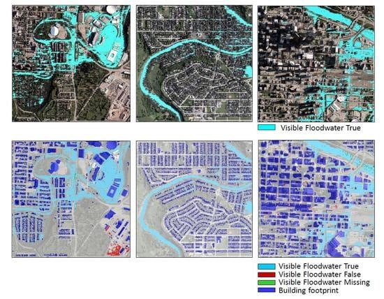
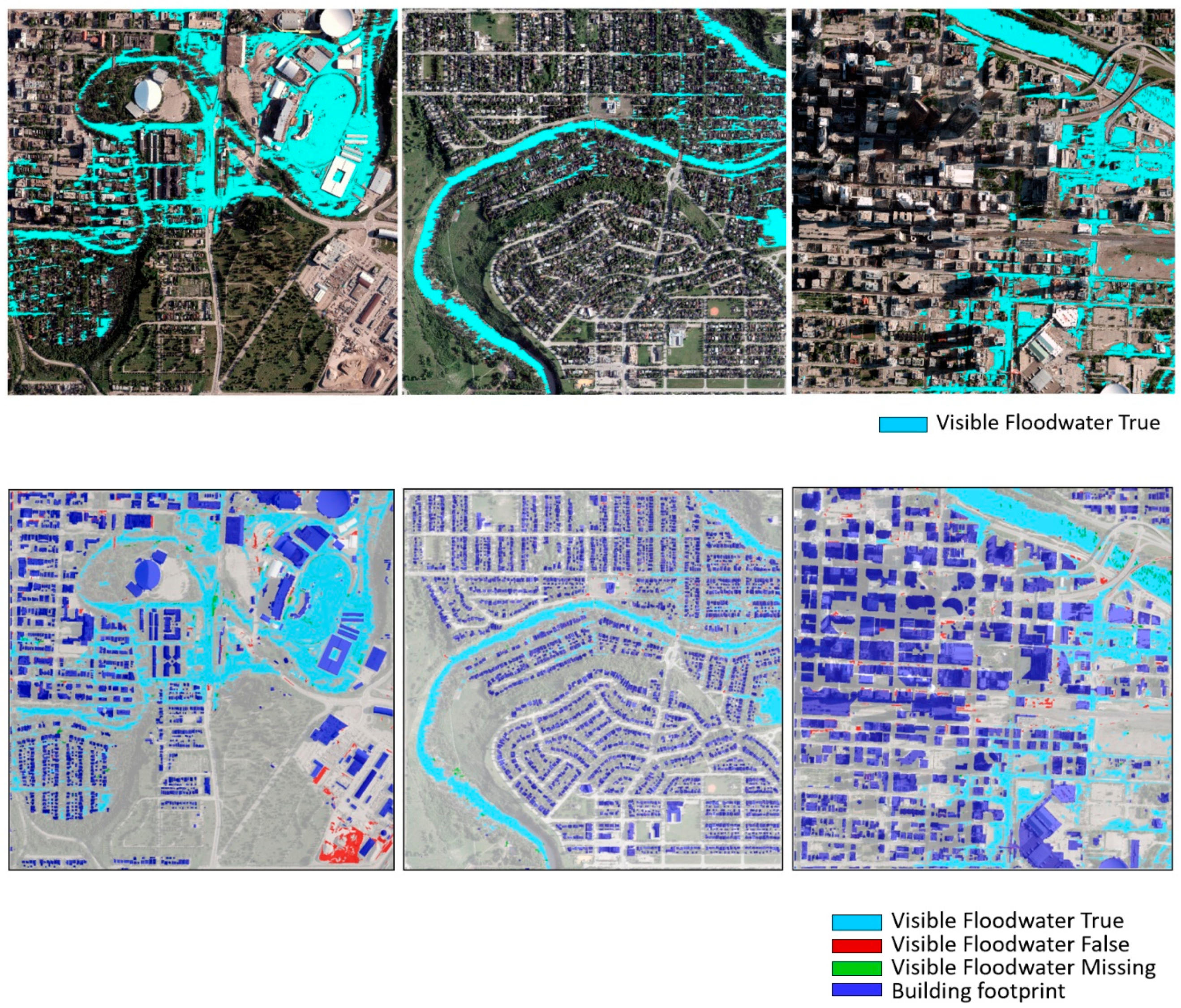
In addition, maps of floodwater class errors are shown in Figure 10, where the “visible floodwater true” class was the visible floodwater correctly classified, the “visible floodwater false” class was the non-visible flooded areas classified as visible floodwater, and the “visible floodwater missing” class was the visible floodwater classified as non-visible floodwater. The overall accuracies for the three test sites were satisfactory (all above 96%) at both the segment and the pixel levels. There were cases where the accuracies at the segment level were lower than those at the pixel level. This arose primarily from incorrectly classified small segments. Another error arose in the case of wet soil which was highly confused with floodwater due to high spectral similarities. A large patch of floodwater class errors was found in site A where a light industrial site included a region of bare wet soil. Overall, in dense urban areas such as those in the Calgary case, there were few land surfaces covered with wet bare soil since (a) the image acquisition was not immediately after rainfall, and (b) there are very few bare soil areas in urban areas during warm seasons except at construction sites.

Considering that the visible floodwater extracted from remote sensing imagery is only a portion of the real flooded area, a comparison of the visible floodwater map with the total flooded area map was made. The total flooded area map was manually generated by the City of Calgary with ground-truth information. The percentages of the visible floodwater portion were estimated for test sites. Visible floodwater percentages were estimated to be 43.56%, 30.58%, and 53.49% for sites A, B, and C, respectively. This indicates that the percentages of flooded areas under tree canopies and in shadows were significant in the Calgary case. Although the percentage of the visible floodwater was not high, the visible floodwater extracted was a critical information source as it could be used as a key clue for further inference of the real floodwater extent (i.e., including the flooded areas under trees and in shadows, in addition to the visible floodwater) in dense urban areas [28]. Details about our investigation on the inference of real flooded areas will be presented in a later paper.

DEM data were used to correct some of the commission errors, namely, those apparent floodwater patches located at high elevations above the known maximum floodwater level. However, there remained uncertainty regarding commission areas below this maximum level. This was complicated by the fact that, in urbanized areas, there are additional drainage infrastructures and local human activities such as damming that can impact flood levels. Therefore, there are potentially large uncertainties associated with using DEM data only for the prediction of floodwater distribution.

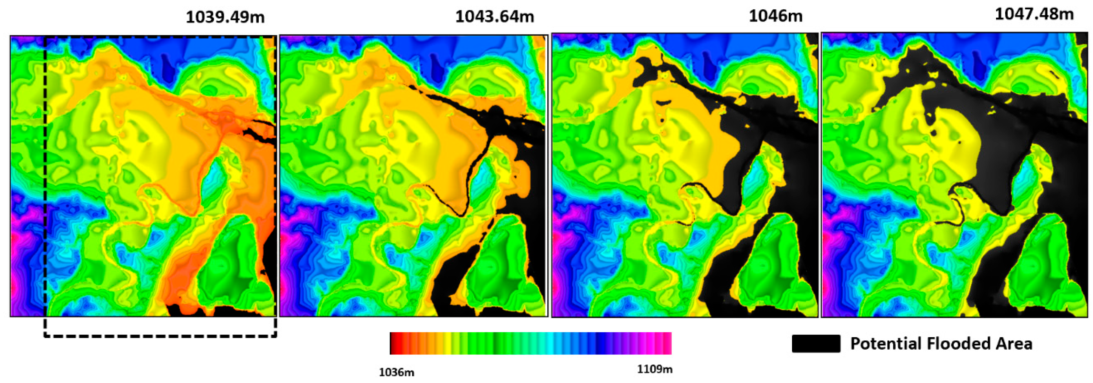
In the Calgary flood case study, maps of possible flooded areas estimated using the DEM alone were compared with the map of the visual flooded areas extracted from the aerial data. The maps of possible flooded areas estimated using the DEM with reference water levels ranging from 1036.0 m to 1047.48 m are presented in Figure 11. Comparing the image-based (Figure 7) and DEM-based flood (Figure 11) coverages, it can be seen that there were obvious differences in the patterns between the real visible floodwater distribution and the predicted distributions based on DEM level. In urban areas with complex landscapes, the floodwater distribution in reality should be influenced by various physical processes and possible human interventions. Therefore, the estimation of the flooded areas using only the DEM can be considered to be of limited value in urbanized areas, especially dense urban areas. The detection of the visible floodwater is the key step for understanding the real floodwater patterns and extent.

Building roofs, constructed from various types of materials, are a major source of commission errors. The use of building footprint data can potentially mitigate this problem. However, a major challenge in using the footprints of very high buildings is the positional horizontal shift of their roof outlines relative to imagery if the image in question was acquired using an off-nadir sensor configuration and not corrected to a proper orthographic projection (a situation likely to be the case in real flood analysis conditions). The reduction of confusion errors using building footprint data, therefore, will not be as effective, especially in downtown business districts and in areas with high-rise apartment complexes.

6. Summary

This paper presented and evaluated a method for the extraction of visible floodwater coverage from RGB aerial imagery over dense urban areas. Visible floodwater denotes the floodwater on the ground surface that can be observed by remote sensing and is a key information source for the analysis of real-time floodwater extent; floodwater under tree canopies and in shadows was excluded from the visible floodwater class. The method was tested using a dataset collected for the flood event in Calgary, Canada in June 2013. A new spectral index, the floodwater index was proposed for optimized separation of the visible floodwater class pixels or image segments from other urban land surface features. In addition, the minimum RGB spectral distance to reference floodwater samples was used as an additional constraint for high mapping accuracy generation. DEM and building footprint data were used for confusion error filtering. For three test sites in the Calgary case study, the overall accuracies at the segment and pixel levels for visible floodwater extraction were above 96.68%. The mean accuracy for the visible floodwater was above 83.94%.

Several important conclusions about visible floodwater mapping using RGB aerial data are discussed below.

Very high-resolution aerial RGB imagery (such as that from imagers carried by aircraft and UAVs) can provide the source of information for rapid response mapping of visible floodwater distributions, despite the limited spectral dimensionality of visible (RGB) data.

The floodwater index developed in this study can be used as a primary tool for rapid extraction of the visible floodwater from RGB image data. Other parameters such as the minimum RGB distance to the floodwater samples, as well as the high-resolution terrain elevation and the building footprint information, can be used as important constraints for increasing the mapping accuracy for dense urban areas.

Although terrain elevation is a parameter influencing the spread of floodwater, the patterns of floodwater extent in dense urban areas generated using the terrain elevation information alone cannot match well to those from the image-based mapping. Therefore, in the estimation of the flood extent in an urbanized area, a DEM can be employed as an ancillary information source but is insufficient as a standalone layer for accurate estimation.