Generation of a Global Spatially Continuous TanSat Solar-Induced Chlorophyll Fluorescence Product by Considering the Impact of the Solar Radiation Intensity

Abstract

Solar-induced chlorophyll fluorescence (SIF) provides a new and direct way of monitoring photosynthetic activity. However, current SIF products are limited by low spatial resolution or sparse sampling. In this paper, we present a data-driven method of generating a global, spatially continuous TanSat SIF product. Firstly, the key explanatory variables for modelling canopy SIF were investigated using in-situ and satellite observations. According to theoretical and experimental analysis, the solar radiation intensity was found to be a dominant driving environmental variable for the SIF yield at both the canopy and global scales; this has, however, been neglected in previous research. The cosine value of the solar zenith angle at noon (cos (SZA₀)), a proxy for solar radiation intensity, was found to be a dominant abiotic factor for the SIF yield. Next, a Random Forest (RF) approach was employed for SIF prediction based on Moderate Resolution Imaging Spectroradiometer (MODIS) visible-to-NIR reflectance data, the normalized difference vegetation (NDVI), cos (SZA₀), and air temperature. The machine learning model performed well at predicting SIF, giving R² values of 0.73, an RMSE of 0.30 mW m⁻² nm⁻¹ sr⁻¹ and a bias of 0.22 mW m⁻² nm⁻¹ sr⁻¹ for 2018. If cos (SZA₀) was not included, the accuracy of the RF model decreased: the R² value was then 0.65, the RMSE 0.34 mW m⁻² nm⁻¹ sr⁻¹ and an bias of 0.26 mW m⁻² nm⁻¹ sr⁻¹, further verifying the importance of cos (SZA₀). Finally, the globally continuous TanSat SIF product was developed and compared to the TROPOspheric Monitoring Instrument (TROPOMI) SIF data. The results showed that the globally continuous TanSat SIF product agreed well with the TROPOMI SIF data, with an R² value of 0.73. Thus, this paper presents an improved approach to modelling satellite SIF that has a better accuracy, and the study also generated a global, spatially continuous TanSat SIF product with a spatial resolution of 0.05°.

1. Introduction

Solar-induced chlorophyll fluorescence (SIF) within the wavelengths ranging from 650 to 850 nm, and which has two peaks centered at 685 and 740 nm [1], is well known as a good proxy for photosynthetic activity [2,3]. Numerous studies have shown that the gross primary productivity (GPP) of vegetation photosynthesis can be directly estimated using satellite, airborne, in-situ and ground level SIF data [4,5,6,7,8,9].

Existing satellite fluorescence products include the Scanning Imaging Absorption spectrometer for Atmospheric CHartographY (SCIAMACHY), Greenhouse gases Observing SATellite (GOSAT), Global Ozone Monitoring Experiment-2 (GOME-2), Orbiting Carbon Observatory-2 (OCO-2), Chinese Carbon Dioxide Observation Satellite (TanSat) and TROPOspheric Monitoring Instrument (TROPOMI) datasets. The first global fluorescence map is based on data acquired by the GOSAT satellite, which has a circular footprint and a spatial resolution of 10.5 km. However, due to the point observation, spatial sampling frequency and the low accuracy of single observations, the average spatial resolution of monthly satellite products is 2° × 2° [10,11,12]. The spatial resolution of the SCIAMACHY satellite is 30 × 240 km (30 km × 60 km in nadir mode), whereas the average spatial resolution of daily satellite products is 1.5° × 1.5° [10,13,14,15]. Because GOME-2 carries out continuous sampling, the same as for SCIAMACHY, the spatial resolution of its synthetic fluorescence products is higher than that of GOSAT, and is about 0.5° × 0.5° [13,15,16]. TROPOMI, with a spatial resolution of 3.5 km × 7 km and a swath of 2600 km, has produced daily global coverage since February 2018 [17,18].

Apart from TROPOMI, the satellite SIF products described above are limited either by low spatial resolution or sparse sampling, and are severely disturbed by noise at low signal levels, which makes it difficult to use then for ecosystem monitoring [17]. The OCO-2 and TanSat SIF data, which have much smaller footprints (i.e., 1.3 × 2.25 km and 2 × 2 km), provide the chance of linking satellite SIF to flux tower-based GPP at the ecosystem scale [19,20]. However, due to the sparse sampling, these data cannot be used for small-region applications in all parts of the globe. Therefore, the spatial expansion of high-resolution SIF data from OCO-2 and TanSat is of great significance for GPP estimation [21,22].

SIF can be expressed as [23,24,25]

$$\begin{array}{c}SIF=PAR·fPAR·SI{F}_{yield}\end{array}$$

(1)

where PAR is the downwelling photosynthetically active radiation (PAR), $fPAR$ is the fraction of PAR absorbed by vegetation, and $SI{F}_{yield}$ is the fluorescence quantum yield at the canopy level.

The SIF contains plant physiological and structural information together with the mixed effects of vegetation biochemistry (i.e., pigments) and structure [26,27], whereas the reflectance provides only canopy structural and biochemic information. $SI{F}_{yield}$, influenced by vegetation biochemistry, contains plant physiologic information. While $fPAR$, which can be estimated using reflectance data, mainly contains vegetation structural information. Zhang et al. [22] and Gentine and Alemohammad [28] constructed the relationship between reflectance and SIF, and reflectance only contains vegetation structural information. Other researchers have taken the land-cover type, Vapor Pressure Deficit (VPD), air temperature, Evapotranspiration (ET) and Normalized Difference Vegetation Index (NDWI) into consideration [21,29,30,31] in order to better model the SIF; however, this can only provide part of the physiological information provided by the SIF. According to Gu et al. [32], $SI{F}_{yield}$ is affected by NPQ and $q_L$, and the solar radiation intensity is a dominant factor for these two physiological variables. However, the solar radiation intensity has not been taken into account in recent prediction models [21,22,31], which has resulted in there being very limited physiological information in the currently available continuous OCO-2 SIF products.

The aims of this study were: (1) to investigate whether the solar radiation intensity, approximated by the cosine value of the solar zenith angle at noon, can provide good physiological information of SIF; (2) to generate global, continuous TanSat SIF products with a spatial resolution of 0.05°; and (3) to investigate the accuracy of spatially continuous TanSat SIF products.

2. Materials and Methods

2.1. Satellite-Based Datasets

2.1.1. TanSat SIF Product

TanSat is the first sun-synchronous satellite that has the potential to retrieve SIF in China and has a revisit period of 16 days. The high spectral resolution (0.044 nm) and high SNR (360 at 15.2 mW m⁻² nm⁻¹ sr⁻¹) of the Atmospheric Carbon dioxide Grating Spectroradiometer (ACGS) in the region of the O²-A band (758–778 nm) provide the potential to retrieve SIF. The TanSat SIF dataset used in this study (https://zenodo.org/record/3883434) was provided by Du et al. [20], and consisted of SIF retrievals (referenced at 758 and 771 nm) retrieved at 13:30 local time. Singular vector decomposition (SVD) was used for SIF retrieval and the surrounding area covering a footprint of 2 × 2 km. TanSat can work in nadir, sun-glint or target mode. However, there was a change from sun-glint mode to nadir mode from October 2018, so the available data for 2019 is equivalent to that for 2017 for the first five months only.

Previous studies have shown that the SIF at different wavelengths has a different sensitivity to stress, and to leaf and canopy reabsorption [33,34,35]. We chose the 758 nm fluorescence because it is closer to the peak band and has a stronger fluorescence signal. In addition, studies have shown that the SIF at 757 nm is better at predicting GPP than the 771 nm SIF [36]. Observations covering the period from February 2017 to August 2019 made at nadir were used in this study to avoid the potential impact of the viewing geometry, as the glint mode tends to underestimate SIF [7].

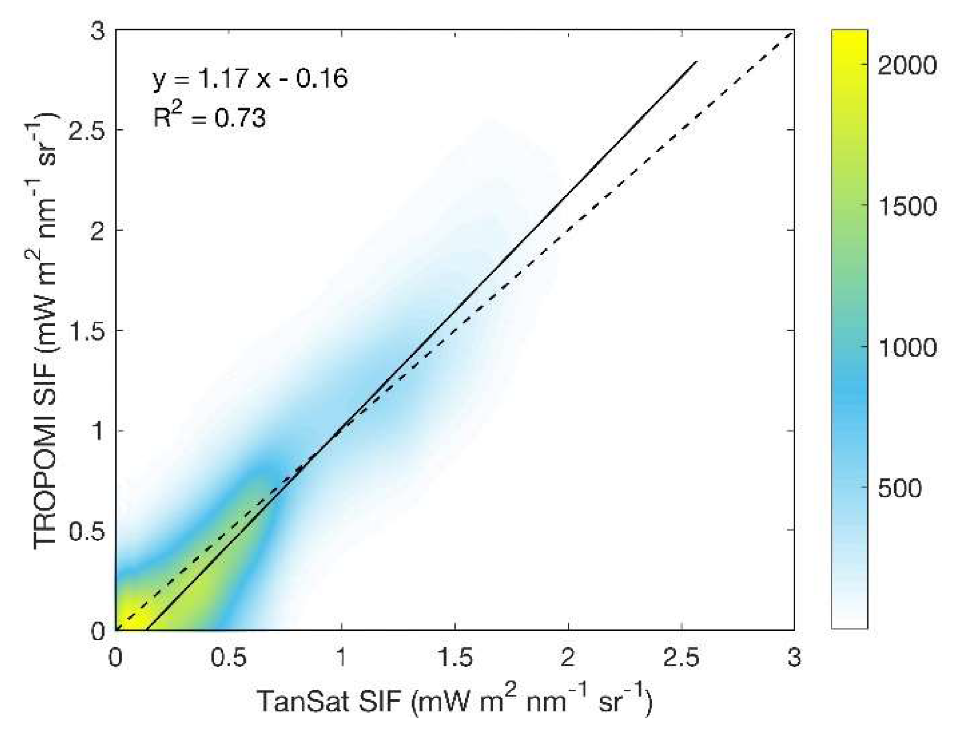
2.1.2. TROPOMI SIF Product

The TROPOMI instrument is carried on-board the Sentinel 5 Precursor (S-5P) satellite [37], which has a crossing time of 13:30 local solar time and a revisit time of 17 days. Available ungridded SIF data with a footprint of 3.5 × 7 km is available from February 2018 and gridded data with a spatial resolution of 0.2° × 0.2° is available from March to October 2018 [18]. For each 0.2° grid cell, if the footprint of the sample covered the center of the cell, this sample was used to calculate the SIF [18].

As the crossing time for TROPOMI is the same as that for TanSat and because it provides almost complete global coverage, 0.2° Tropomi SIF data were used for comparison with the continuous TanSat SIF produced in this study.

2.1.3. MODIS NBAR Reflectance Product

The MODIS Collection 6 Nadir Bidirectional reflectance distribution Adjusted Reflectance (NBAR) product (MCD43C4) was employed to explain the SIF structural information. The BRDF product uses a combination of Terra and Aqua data over a period of 16 days to generate the highest possible quality data for each day. The NBAR product has a spatial resolution of 0.05° × 0.05° and computes the reflectance at a nadir viewing angle for each pixel at local solar noon, which should result in a more stable and consistent product [38].

As the swath width of TanSat satellite is narrow and the selected samples were acquired in nadir mode, the use of NBAR was considered reasonable. Additionally, only four bands of MCD43C4 (red, NIR, blue and green) were used as explanatory remote sensing variables in the modelling of the SIF, which is the same as in Zhang et al. [22] and Gentine and Alemohammad [28]. These four bands contain most of the vegetation information and drive most of the variation in the SIF [39]. In order to reduce the uncertainty in modelling the SIF, only high-quality MCDC43C4 data (Quality = 0) were used.

2.1.4. Air Temperature Datasets

Air temperature products can be used to provide physiological information for vegetation [31]. In this study, we used GLDAS/Noah L4 3-hourly 0.25-degree products (download address: http://disc.sci.gsfc.nasa.gov/hydrology/data-holdings). At the basin scale (14,700 km²), this highly accurate temperature product is suitable for water and energy-cycling studies [40,41]. The GLDAS data, acquired at 3-h intervals, was produced on February 24, 2000; a detailed description can be seen in Rodell et al. [42].

2.2. Tower-Based Datasets

We used both satellite and tower-based data to obtain the relationship between $SI{F}_{yield}$ and cos (SZA₀). The SIF inversion was based mainly on the Fraunhofer Line Depth (FLD) and the Spectral Fitting Method (SFM). The tower-based cropland SIF dataset used in this study was acquired at the Huailai, Daman and Aurora sites [43,44,45]. The canopy SIF data from Huailai and Daman covered the period from July to September in both 2017 and 2018, and from April to October in 2019. The canopy SIF dataset in maize field from Aurora site covered the period from July 2018 to September 2018 (doi: 10.22002/D1.1226), which are available from California Institute of Technology (https://data.caltech.edu/records/1226) [45]. Another canopy SIF dataset that was used was acquired at the Niwot Ridge site from June 2017 to June 2018; the major species here is evergreen needleleaf. This needle-scale SIF data (doi: 10.22002/D1.1231) are available from the California Institute of Technology (https://data.caltech.edu/records/1231) [9].

In total we acquired 372 samples from the Huailai and Daman sites, 209 samples from the Niwot Ridge site and 57 samples from the Aurora site.

Table 1. Details of the Eddy Covariance (EC) flux sites.

Ecosystem Type	Site Name	ID	Latitude	Longitude	Height
Cropland	Huailai	HL	40.35°N	115.79°E	4 m H
	Daman	DM	38.86°N	100.37°E	25 m H
	Aurora	-	42.72°N	76.66°W	7 m H
Forest	Niwot Ridge	NR	40.03°N	105.55°W	26 m H

shows the detailed information of these sites.

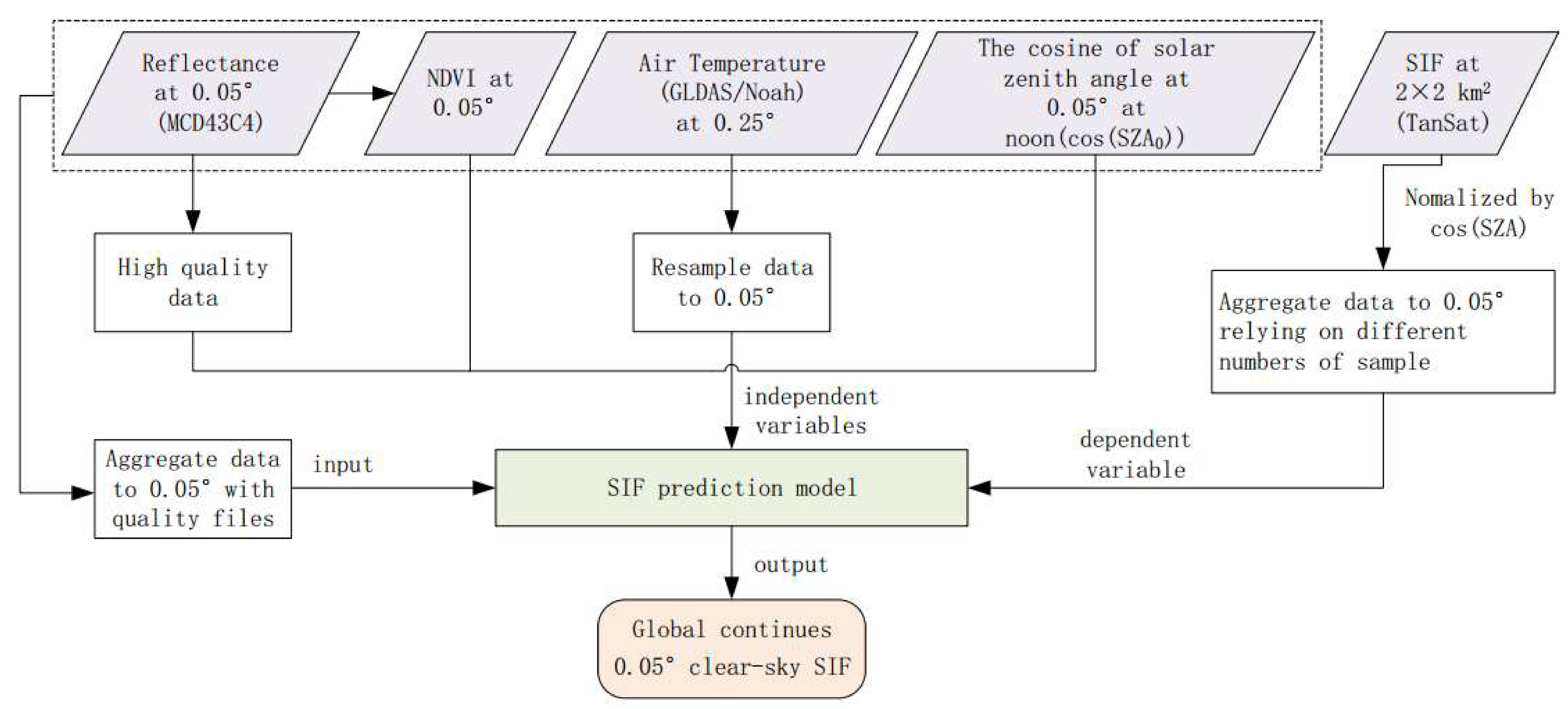
2.3. Data-Driven SIF Prediction Model Using the Random Forest Algorithm

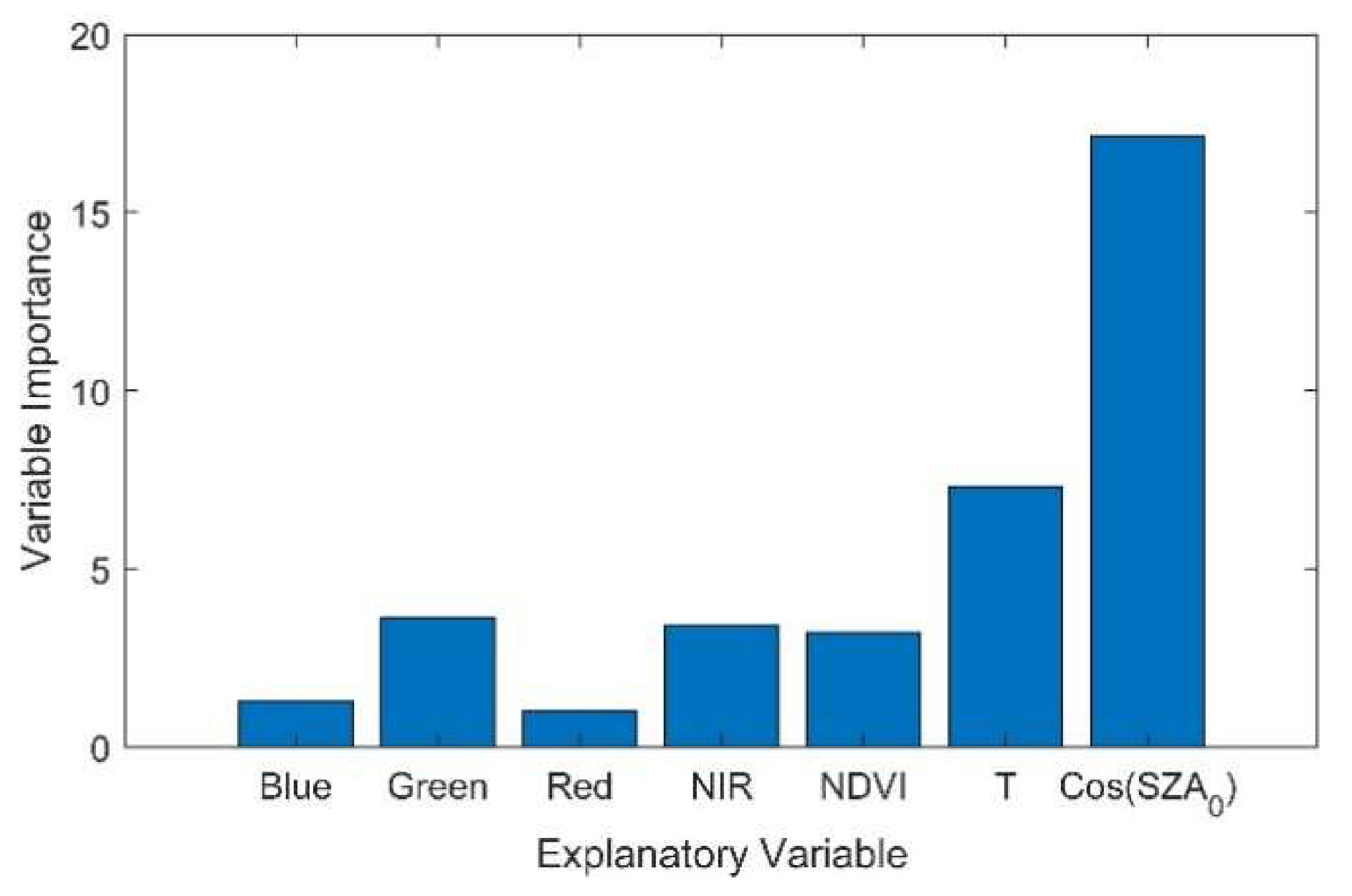
2.3.1. Explanatory Variable Selection for SIF Prediction Model

According to Gu et al. [32], the SIF can be calculated as:

$$\begin{array}{c}SIF=PAR·\epsilon {\alpha }_{gm}·{\Phi }_{SIF}\end{array}$$

(2)

where $\epsilon$ is the canopy escape probability of SIF photons, ${\alpha }_{gm}$ is the fraction of PAR absorbed by green leaves, and ${\Phi }_{SIF}$ is the fluorescence quantum yield.

This formula can be divided into three terms: $PAR$, $\epsilon {\alpha }_{gm}$ (the SIF variation related to the canopy structure) and ${\Phi }_{SIF}$ (the SIF variation related to plant physiological factors). Since the incoming PAR of instantaneous SIF differs according to the location, the SIF normalized by PAR has been widely used to describe the global photosynthetic capability [46,47]. For satellite SIF observations, which are available only under clear-sky conditions, the PAR can be assumed to be linearly correlated with the cosine value of the solar zenith angle at the transit time of the satellite [8,11,48]. $SI{F}_{normalized}$ is the SIF normalized to a fixed transit time, based on the central latitude and longitude of each grid cell (Equation (3)):

$$\begin{array}{c}SI{F}_{normalized}=\frac{SIF}{PAR}=\frac{SIF}{cos\left(SZA\right)}\end{array}$$

(3)

where cos (SZA) is the cosine of the solar zenith angle at the satellite transit time. Then Equation (2) can be written as:

$$\begin{array}{c}SI{F}_{normalized}=\epsilon {\alpha }_{gm}·{\Phi }_{SIF}\end{array}$$

(4)

At the far-red band, $\epsilon$, the canopy escape probability of the SIF, is dominated by the canopy bi-directional reflectance (BRF) [25,49,50,51]. ${\alpha }_{gm}$, the FAPAR for green leaves, has been widely estimated using combinations of BRFs [52,53,54]. The second term in Equation (2) depends on the reflectance and vegetation indices (VIs), which are directly related to plant structure. Additionally, since the selected TanSat SIF was acquired nadir mode, it was reasonable to assume that $\epsilon {\alpha }_{gm}$, which is the contribution of the structural information to SIF, could be modeled using BRDF-corrected reflectance and VIs.

${\Phi }_{SIF}$, which accounts for the contribution of plant physiological factors to SIF, can be determined using chlorophyll fluorescence parameters, which, in turn, can be obtained by pulse-amplitude-modulated (PAM) fluorometry [32]. Since, in this case, the value of PSI SIF was low and stable, PSI was not taken into consideration when calculating ${\Phi }_{SIF}$ [32,33,55];

$$\begin{array}{c}{\Phi }_{SIF}=\frac{1-{\Phi }_{PSIImax}}{\left(1+k_{DF}\right)\left[\left(1+NPQ\right)\left(1-{\Phi }_{PSIImax}\right)+q_L{\Phi }_{PSIImax}\right]}\end{array}$$

(5)

where $k_{DF}$ is the ratio of thermal dissipation ($k_D$) to fluorescence emission ($k_F$), $NPQ$ is the adjustable heat dissipation, $q_L$ is the fraction of photosynthesis system II (PSII) reaction centers, and ${\Phi }_{PSIImax}$ is the maximum photochemical quantum yield of PSII.

In Equation (5), $k_{DF}$ is always assumed to be constant as $k_D$ and $k_F$ are considered to be intrinsic physical properties of the chlorophyll molecule. ${\Phi }_{PSIImax}$ typically ranges from 0.8 to 0.83 and varies slightly under environmental stress [56]. Therefore, ${\Phi }_{SIF}$ mainly depends on $NPQ$ and $q_L$. Numerous studies have shown that $NPQ$ and $q_L$ vary with external conditions and stresses, such as illumination, temperature, and water stress [32,57,58], and that illumination or PAR is the main driving factor for them [32]. In addition, in diurnal experiments carried out on sunny days and investigations into light response, $NPQ$ and $q_L$ have been shown to have a strong relationship with the illumination [32,58,59]. For satellite-based observations, only the SIF on sunny days is available, and so our aim was to produce a global SIF product for clear conditions. Therefore, the cosine of the solar zenith angle at noon (cos (SZA₀)) was used to represent the illumination conditions in this study and for simulating the fluorescence quantum yield ($SI{F}_{yield}$) at the canopy scale.

Therefore, BRDF-corrected reflectances (red, NIR, blue and green bands), NDVI, cos (SZA₀), and the air temperature were selected as explanatory variables for modelling satellite $SI{F}_{normalized}$ signals. Compared to other studies [21,22,29,30,31], it was hoped that adding cos (SZA₀) as a new explanatory variable might improve the modelling of the contribution of ${\Phi }_{SIF}$ to SIF, given the light response of $NPQ$ and $q_L$ to cos (SZA₀). The data-driven model used for reconstructing the normalized SIF was:

$$\begin{array}{c}SI{F}_{normalized}=f\left(Rs,NDVI,cos\left(SZ{A}_0\right),T\right)\end{array}$$

(6)

where NDVI is the normalized difference vegetation index, T is the air temperature, and $Rs$ represents the four BRDF-corrected reflectances at the red, NIR, blue and green bands.

2.3.2. Random Forest Approach for SIF Modeling

Random forest has been widely applied in remote sensing applications such as classification, and the estimation of high-density wetland biomass [60,61,62,63]. Random forest (RF) was first proposed by Leo Breiman [64] and is a classifier that uses multiple decision trees to train and predict samples. Compared with other widely used non-parametric algorithms, RF is insensitive to unbalanced distributions and the problem of missing data. Because of the random way it selects data for splitting each tree node, it is also less sensitive to the over-fitting problem [60,64]. It performs better for large, high-dimensional data sets and is more robust to noise and feature selection [34,61,62,63,65]. Additionally, the prediction ability of Random Forest is resistant to the multicollinearity of the driven variables [66,67,68], so all the all the variables in Equation (2) were used to predict the spatially continuous TanSat SIF. The main parameters used in RF are the numbers of input prediction variables and decision trees. Gislason et al. [69] found that there was no obvious relationship between the accuracy and the number of selected prediction variables, and so used the default value of the square root of the total number of variables [62,70]. For the number of decision trees, Du et al. [71] found by developing 10 to 200 trees (at intervals of 10) that the accuracy was insensitive to the number of trees. In this study, 100 trees and six variables (three prediction variables were selected) were used in RF. The importance of each predictor was calculated by calculating the percentage increase in the mean-squared error when the value of a particular variable was changed (while keeping the other values unchanged): this allowed us to determine which were the important variables [64].

Here, a Random Forest (RF) approach was employed to model the normalized SIF, as in Equation (6): the flowchart for the corresponding procedure is illustrated in Figure 1. The input variables used were MCD43C4, and the vegetation index, air temperature and cos (SZA₀) datasets. Since the spatial resolution of MCD43C4 is 0.05°, to maintain consistency with MCD43C4, the TanSat SIF needed to be aggregated to a resolution of 0.05°. The SIF training samples were eliminated if there were less than 20 samples in each 0.05° cell between 10°S and 60°N. However, due to the low vegetation coverage in some areas, there were few valid data. Therefore, in order to keep the integrity of the global coverage of the samples, we relaxed these restrictions and only eliminated samples which had less than 5 samples in each grid cell. The final results were that there were 118,722 SIF grid cells for 2017, 187,077 cells for 2018, and 173,153 cells for 2019. The air temperature data were also resampled to 0.05 degrees using polynomial interpolation.

To validate the RF model, we randomly took 70% of the data as the training set and 30% as the validation set for each year. Three accuracy metrics, the coefficient of determination (R²), Relative Deviation (RD) and Root Mean Square Error (RMSE) were used to evaluate the performance of the RF model.

3. Results

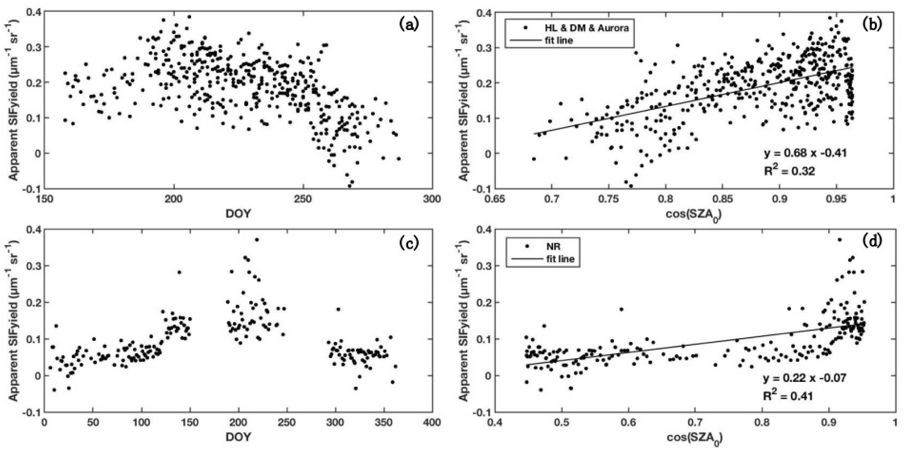
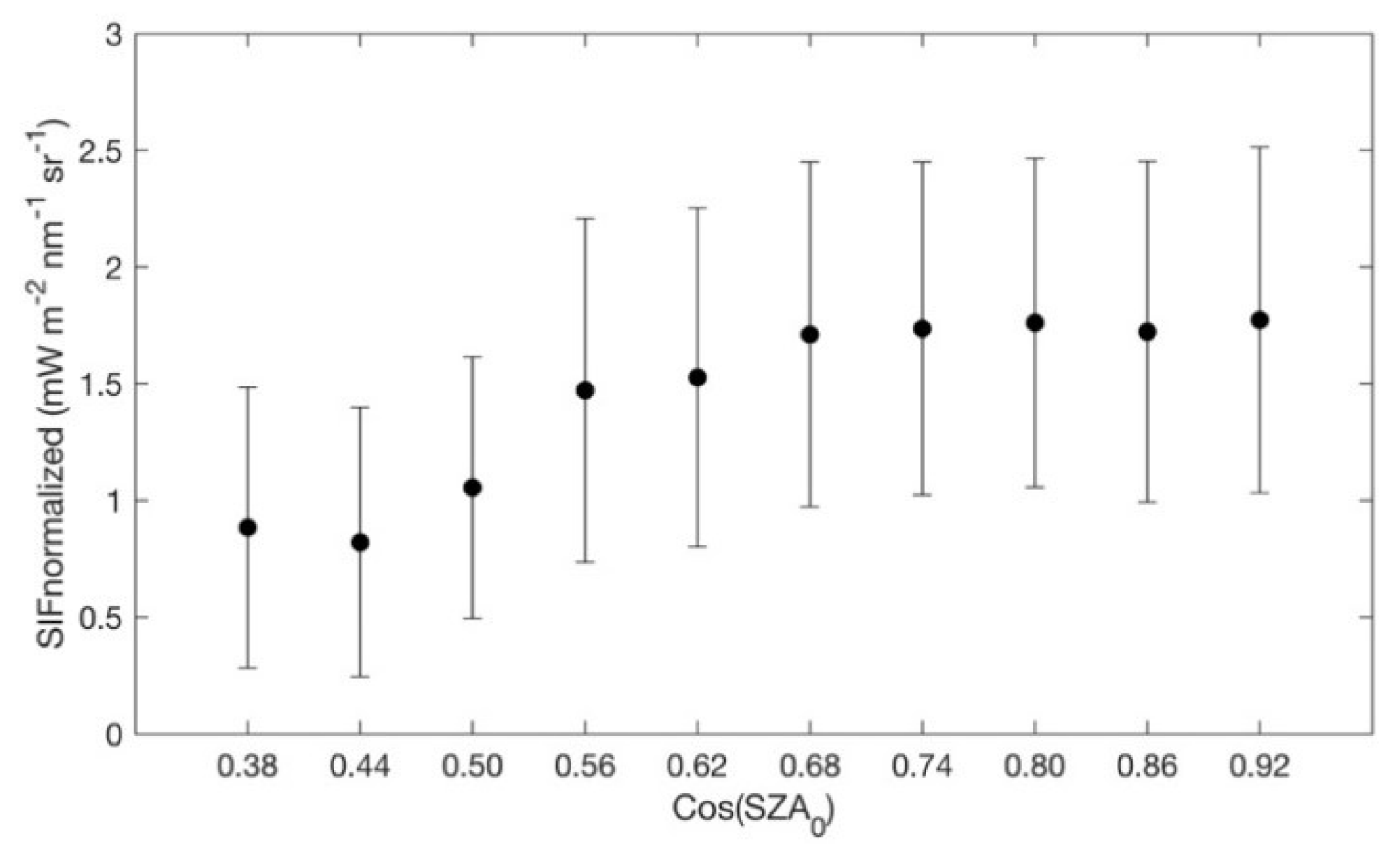
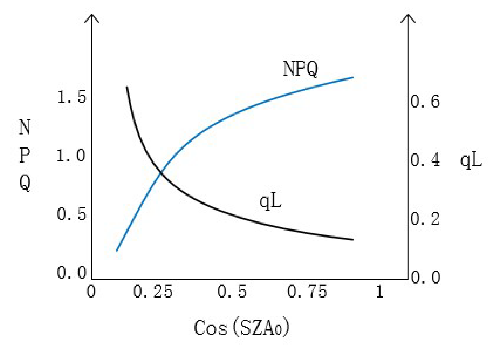
3.1. Relationship between cos (SZA₀) and Apparent SIF Yield

The tower-based and satellite experimental data were used to investigate the relationship between the apparent $SI{F}_{yield}$ (calculated using the SIF observed at the top of the canopy) and cos (SZA₀). As illustrated in Figure 2, there was a seasonal change in the apparent $SI{F}_{yield}$, which was correlated with cos (SZA₀) in the maize crop and evergreen forest ecosystems. Therefore, it was concluded that cos (SZA₀), which is a proxy for the solar radiation intensity, could be used to describe the seasonal variation in the apparent $SI{F}_{yield}$.

From Figure 2a,c it can be seen that the value of apparent ${\mathrm{SIF}}_{\mathrm{yield}}$, reaches its peak in July. As illustrated in Figure 2b,d, the apparent ${\mathrm{SIF}}_{\mathrm{yield}}$ also increases as cos (SZA₀) increases at the crop sites (slope = 0.68, R² = 0.32) and the NR forest site (slope = 0.22, R² = 0.41). The different values of the slope may be due to the different types of ecosystem and number of samples. As has been widely observed previously, the value of apparent $SI{F}_{yield}$ at the canopy level was higher for cropland than for forest [72,73].

The relationship between apparent $SI{F}_{yield}$ and cos (SZA₀) was also investigated using the TROPOMI SIF data acquired from February 2018 to February 2019. As in-situ APAR data were not available for TROPOMI SIF, $SI{F}_{normalized}$ (as defined in Equation (3)) for dense vegetation (NDVI > 0.85) was used as a proxy of the apparent $SI{F}_{yield}$. Only forest pixels lying within the area of dense vegetation (NDVI > 0.85) were selected. The dense vegetation regions at DOY 210 and 365 in 2018 were illustrated in Figure 3.

Then, we calculate $SI{F}_{normalized}$. The values of cos (SZA₀) were divided into 10 levels ranging from 0.35 to 0.95. The results showed an obvious rise in $SI{F}_{normalized}$ with cos (SZA₀) at the global scale (Figure 4), indicating the important influence of the solar radiation intensity on apparent $SI{F}_{yield}$.

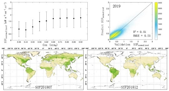
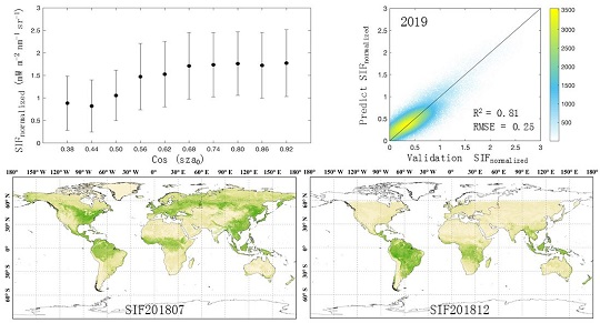
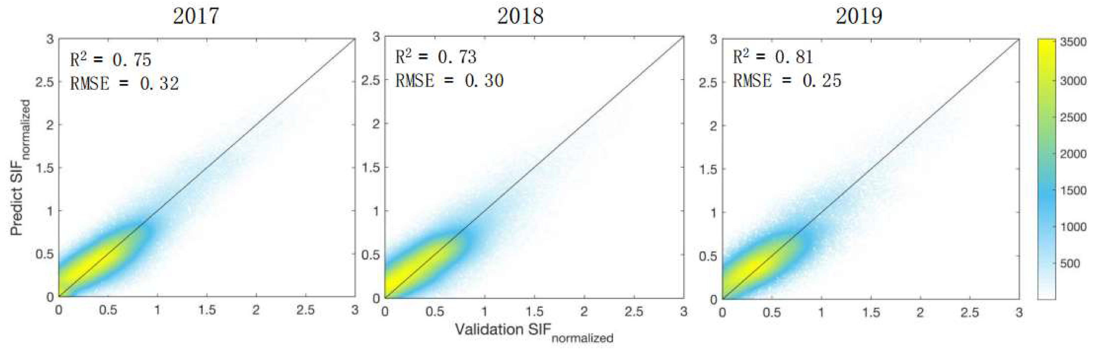
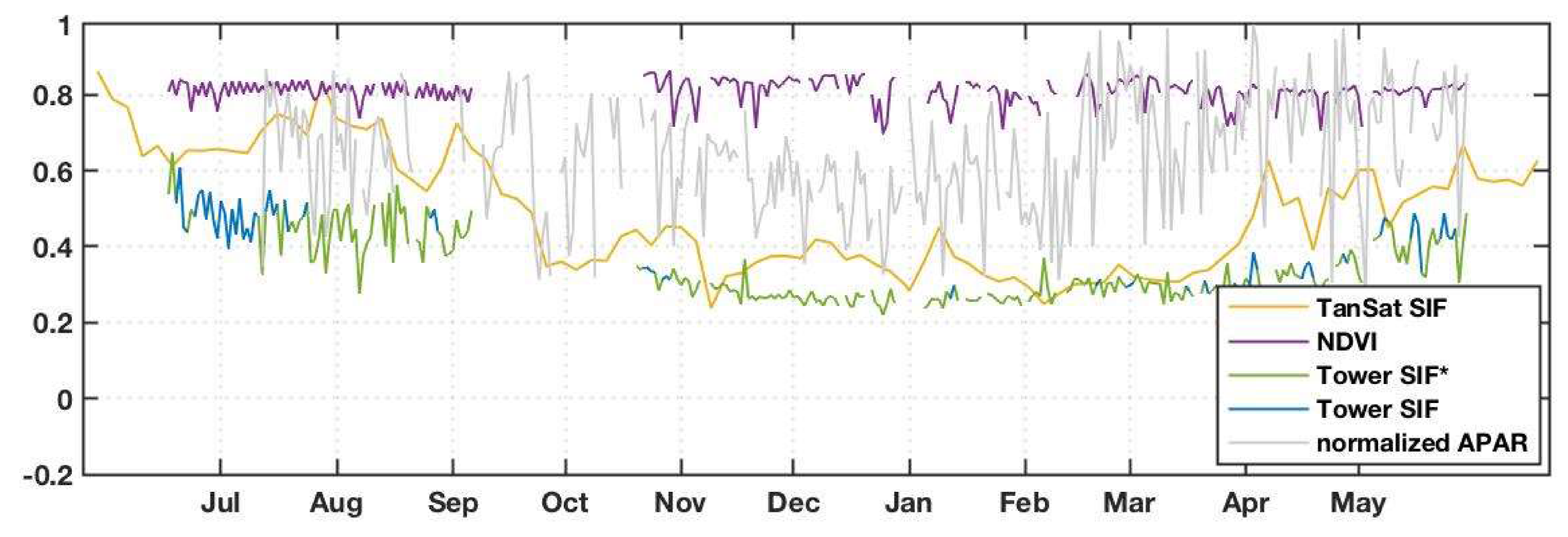
3.2. Performance of the Random Forest Model in SIF Prediction

To better understand the performance of explanatory variables for $SI{F}_{normalized}$, we calculated the importance of the variables in the model using RF; the results are shown in Figure 5.

Figure 5 shows that cos (SZA₀) and the air temperature proved to be the most important input parameters for $SI{F}_{normalized}$; the green and NIR reflectance and NDVI were the next most important. Healthy plants have a high reflectivity in the NIR band. The results for the performance of RF with six explanatory variables are shown as Figure 6.

The results show that the RF model performed well at simulating TanSat SIF (Figure 6), with R² values of 0.75, 0.73 and 0.81, RMSE values of 0.32, 0.30 and 0.32 mW m⁻² nm⁻¹ sr⁻¹, and RD values of -0.32, 0.02 and −0.14 mW m⁻² nm⁻¹ sr⁻¹, for the 2017, 2018 and 2019 datasets, respectively.

A comparison between models that did and did not include cos (SZA₀) was also made. Taking the 2018 dataset, for example, the RF model gave a better accuracy if cos (SZA₀) was included, giving an R² of 0.72, an RMSE of 0.30 mW m⁻² nm⁻¹ sr⁻¹ and an bias of 0.22 mW m⁻² nm⁻¹ sr⁻¹; this was against an R² of 0.65, an RMSE of 0.34 mW m⁻² nm⁻¹ sr⁻¹ and an bias of 0.26 mW m⁻² nm⁻¹ sr⁻¹ without cos (SZA₀). In comparison, R² was improved by 0.07, RMSE was reduced by 0.04, and bias was reduced by 0.04.

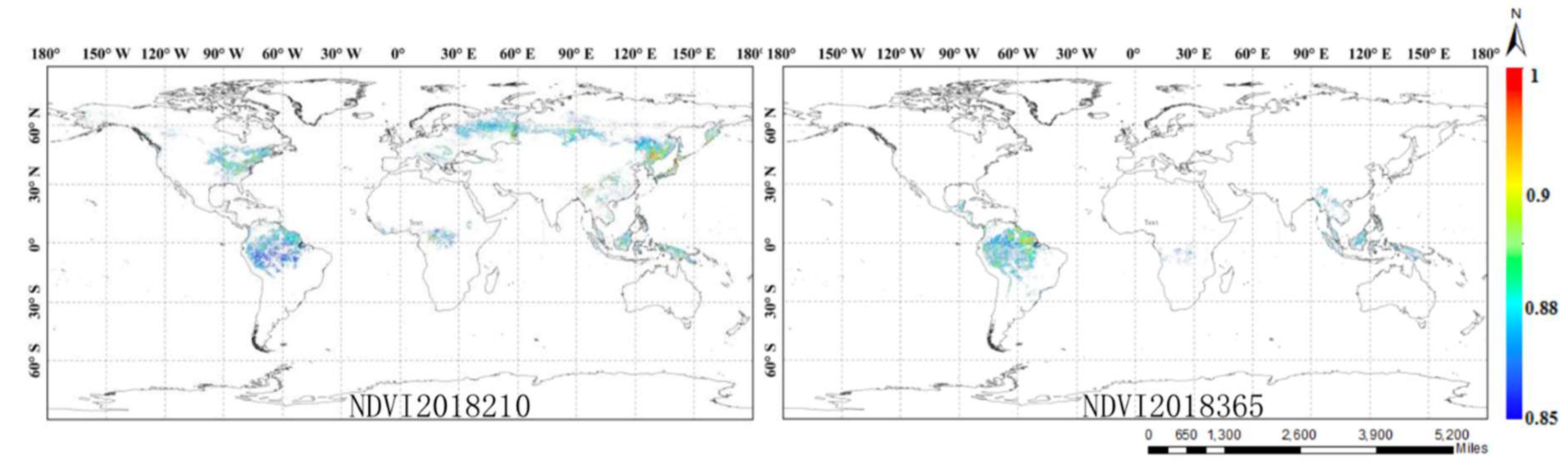
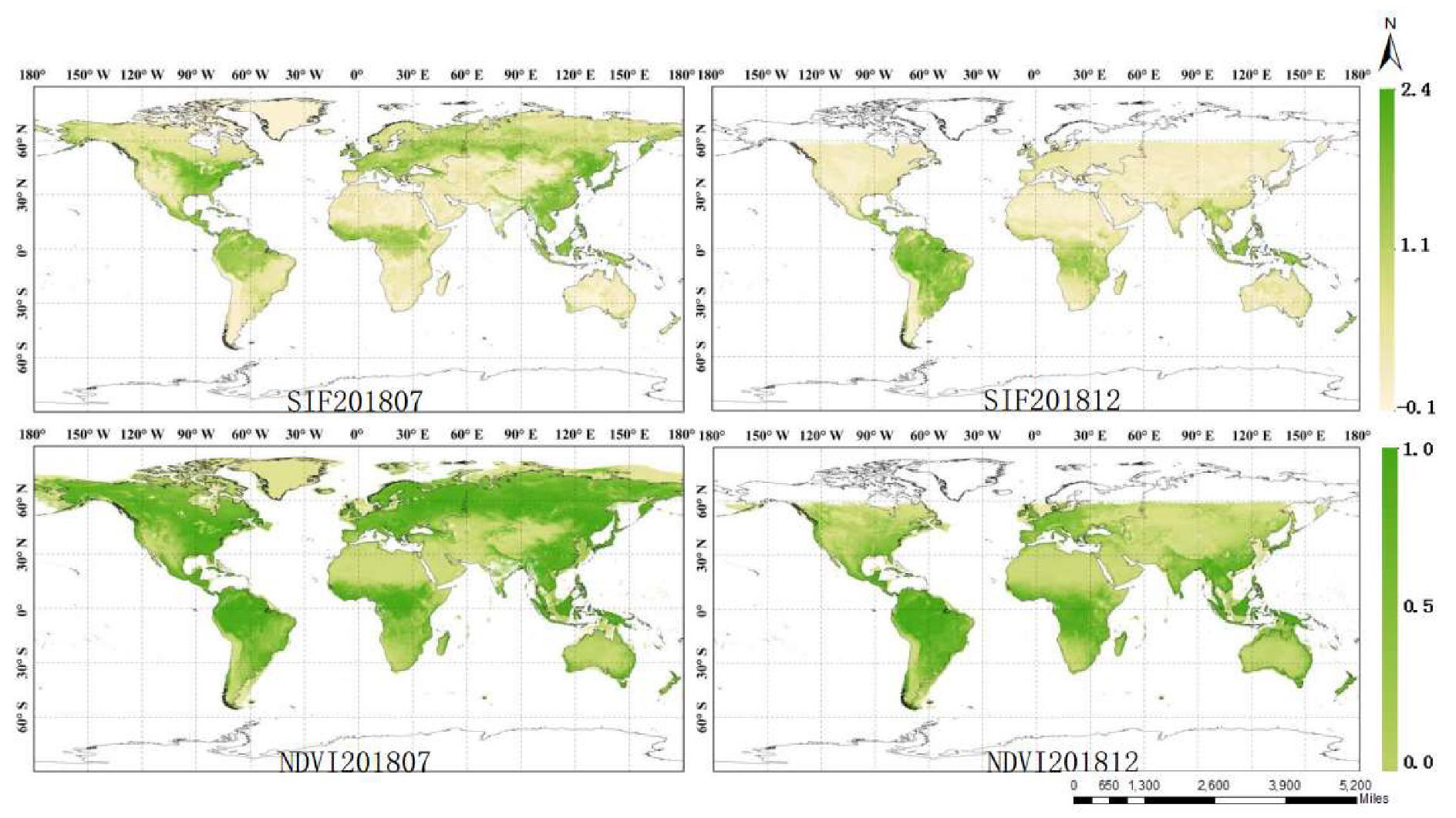
3.3. Global Continuous TanSIF Product

Based on the RF model, a global, continuous SIF dataset that included cos (SZA₀) at the transit time for the central latitude and longitude of each grid cell, normalized to the same level (0.2° × 0.2°) as TROPOMI for the period 2017–2019 was produced. This dataset had a spatial resolution of 0.05° and a temporal resolution of four days. Figure 7 shows the spatially continuous TanSat SIF products for July and December in 2018, together with the NDVI for comparison. Tropical rainforest areas had high SIF values in both July and December. In July, southeast and northeast China, the eastern United States, and southern Europe as well as southern Russia were hot spots of SIF, which agrees well with the distribution of dense vegetation.

Since the transit time of TanSat and TROPOMI was almost the same at about 13:00 local time, the continuous TanSat SIF data were also validated using TROPOMI SIF data. In order to reduce the impact of noise, 0.05-degree TanSat SIF was aggregated to 0.2-degrees so that it could be compared with 0.2-degree TROPOMI SIF, as produced by Koehler et al. [18]. The comparison is illustrated in Figure 8. Since TROPOMI SIF is retrieved at around 740 nm, it has a higher value than TanSat SIF, which is retrieved at 758 nm. R² was used to evaluate the consistency between the two data sets. The results show that the continuous TanSat SIF dataset agreed well with the TROPOMI SIF with an R² of 0.73, indicating that the SIF can be well modeled by integrating cos (SZA₀) with other metrics.

The values of TanSat SIF were all lower than 2.5 mW m⁻² μm⁻¹, whereas the maximum value of TROPOMI SIF reached around 6 mW m⁻² μm⁻¹. Compared with TROPOMI SIF at 740 nm, TanSat SIF at 758 nm was obviously lower in the high (>1 mW m⁻² μm⁻¹) fluorescence region but higher where the fluorescence was around 0.1–0.5 mW m⁻² μm⁻¹.

4. Discussion

4.1. Importance of Solar Radiation Intensity for Better SIF Modelling

The biggest problem in existing SIF prediction models is that the influence of ${\Phi }_{SIF}$ is not well considered. ${\Phi }_{SIF}$ is mainly determined by heat dissipation ($NPQ$) and the fraction of PSII reaction centers ($q_L$) [32]. $NPQ$ increases as PAR increases, while $q_L$ decreases with increased PAR [59,74,75]. Therefore, the solar radiation intensity should be taken into account for better SIF modelling. The relationship between cos (SZA) and PAR is approximately linear for clear-sky conditions. Based on the above relationship, we have drawn a conceptual diagram that briefly indicates the relationship between cos (SZA₀) and $\mathrm{NPQ}$/${\mathrm{q}}_{\mathrm{L}}$, as Figure 9. For satellite observations, only retrievals at clear-sky conditions were available; therefore, in this study, the cosine of the solar zenith angle at noon (cos (SZA₀)) was used to represent the seasonal variation of solar radiation intensity.

The results presented in this paper have confirmed that cos (SZA₀) can be used successfully as a proxy for solar-radiation-intensity information to produce better modelling based on satellite SIF data. A certain degree of correlation was found between cos (SZA₀) and tower-based and satellite SIF apparent yield. The apparent SIF yield increased as cos (SZA₀) increased. Analysis of the importance of different variables using the RF approach clearly showed that cos (SZA₀) was the most important variable for the modelling of $SI{F}_{normalized}$. Therefore, our results were consistent with those of Gu et al. [32], which emphasized that, in theory, the solar radiation intensity is the main factor affecting the apparent SIF yield.

The seasonal trend in SIF at the Niwot Ridge site, where the majority of the forest consisted of needleaved evergreens, was investigated using both continuous TanSat and tower-based SIF measurements made by Magney et al. [76], and also compared with the tower-based NDVI observations, as illustrated in Figure 10. Here, we used the daily mean clearness index (CI) (only CI > 0.6 was used) to determine whether it was clear skies [77]. We calculated the daily SIF under clear-sky conditions, if there are more than three samples a day. We found that the seasonal trend in the continuous TanSat SIF values was consistent with that observed in the tower-based SIF data. The SIF signal reached its peak in summer and remained low in winter. In the first growing season, the slightly difference may be caused by observation error. The low values of SIF for evergreen needleleaf forest in winter season may be caused by snow cover [78]. Combined with in-situ APAR and tower-based SIF under clear-sky conditions, the high value of TanSat SIF may be due to the fact that the contidion of cloudy days was not considered in the model. The differences between TanSat SIF and tower-based SIF may also be due to the time scale and geographic coverage. The TanSat SIF dataset consisted of 0.05-degree instantaneous SIF values acquired at 13:30 local time, whereas the tower-based SIF values used were the daily averages for the station. NDVI was relative stable for all seasons around 0.8. Compared with NDVI, it was found that the SIF can better track seasonal changes in vegetation, which indicates that the spatially continuous TanSat SIF contains more physiological information related to plant photosynthesis.

4.2. Importance of Reflectance and NDVI

Recent studies have used reflectance or NDVI to present most of the vegetation information used in predicting SIF [21,22,28]. In this paper, the main parameter used to provide plant physiological information for the SIF was the solar radiation intensity (as discussed in Section 2.3.1), whereas the reflectance and NDVI were mainly used to provide canopy structure-related information, which was mainly represented by the fraction of PAR absorbed by green leaves in Equation (2).

The canopy structure influences the re-absorption, scattering and escape probability of emitted SIF photons [25,50,79], and the reflectance and NDVI can provide structural information [33,80]. The NDVI was designed to enhance the vegetation information contained in the canopy reflectance. However, the NDVI characteristic may not be well learned by the random forest machine-learning model using red/near-infrared reflectance, although the relationship between the NDVI and the two reflectances is completely deterministic [81,82]. Therefore, the NDVI and red/near-infrared reflectance were both included in the random forest model in this study, although this may seem some redundant.

Gentine and Alemohammad [28] and Yu et al. [21] used seven MODIS reflectance bands to present SIF information. It was found that the first four bands (red, near-infrared, blue and green) can provide most of the vegetation information [39,83]. In our case, we found that the improvement in R² achieved by using seven bands rather than four was less than 0.1, which is consistent with the results found by Zhang et al. [22]. Therefore, only four MODIS reflectance bands were subsequently used in this study.

Near-infrared and red bands are most commonly used to represent the vegetation structural and pigment concentration information. The near-infrared band contains structural information, which influences the SIF escape probability (and also the NDVI) [50,84]. The near-infrared reflectance has a linear relationship with the canopy scattering scale, and has an inverse relationship with the leaf albedo and the amount of light intercepted by the canopy (the complement to the fraction of light that reaches the soil and does not interact with the canopy) [25,26,49] chlorophyll concentration has less impact on the escape ratio and reflectance in the near-infrared SIF [85]. The red reflectance is strongly associated with pigments apart from the xanthophyll carotenoids, and can provide information about the absorption [83,86]. Red radiation is strongly absorbed by chlorophyll, and the absorption increases with chlorophyll concentration [26,87].

The blue and green bands also contain helpful information for predicting SIF. Firstly, reflectance is mainly used to provide information related to fPAR. PAR covers the spectral window from 400–700 nm, which includes the blue, green and red bands. This means that the red band alone cannot well represent fPAR-related information. Secondly, as carotenoids transfer energy to chlorophyll molecules during photosynthesis [76], the use of the blue and green bands can help in the measurement of carotenoid concentration and variation, which are related to the amount of absorption. The blue reflectance is strong related to chlorophyll and carotenoid (including carotenes and xanthophylls) absorption; and green reflectance is sensitive to the difference between two extreme situations of xanthophyll carotenoids with higher absorption [83,86]. Thirdly, the green reflectance slowly changes with the pigment pool size at the seasonal scale [63]. Additionally, the Photochemical Reflectance Index (PRI), which is calculated form the green reflectance, is related to canopy photosynthetic efficiency over different kinds of species and time scales [88,89]. Many researchers have shown that the PRI can represent NPQ [83,90,91].

Therefore, BRDF-corrected reflectance (at the red, near infra-red, blue and green bands) and the NDVI are all important in predictions of SIF, and also provide a certain amount of structural information.

5. Conclusions

In this paper, we have presented an improved approach to modelling satellite SIF by taking the influence of illumination on the SIF_yield into account. The cosine of sun zenith angle at noon (cos (SZA₀)) was used to represent the illumination conditions, and together with the reflectance, NDVI, and air temperature, was used to generate a spatially-continuous TanSat SIF product with a resolution of 0.05° for the period 2017–2019. The results showed that cos (SZA₀) is an important factor affecting the SIF yield. It was also shown that, of the variables in the RF model, cos (SZA₀) was the most important, and that the model accuracy could be significantly improved by including cos (SZA₀) as an explanatory variable. The RF model also modelled the TanSat SIF well (R² = 0.74 for 2017, 0.74 for 2018, and 0.81 for 2019). The global, continuous TanSat SIF data were highly consistent with TROPOMI SIF, with an R² of 0.73. Furthermore, the continuous TanSat product was able to capture the seasonal characteristics of the evergreen needleleaf forest site at Niwot Ridge, where the SIF is low in winter. Therefore, the globally continuous TanSat SIF product contains more physiological SIF information and can serve as a reliable global SIF dataset for monitoring plant photosynthetic activity. And the global spatially continuous TanSat SIF product was available at the zenodo website (https://zenodo.org/record/3884309).

References

1. Pedros, R.; Moya, I.; Goulas, Y.; Jacquemoud, S. Chlorophyll fluorescence emission spectrum inside a leaf. Photochem. Photobiol. Sci. 2008, 7, 498–502. [Google Scholar] [CrossRef] [PubMed] [Green Version]
2. Grace, J.; Nichol, C.; Disney, M.; Lewis, P.; Quaife, T.; Bowyer, P. Can we measure terrestrial photosynthesis from space directly, using spectral reflectance and fluorescence? Glob. Chang. Biol. 2007, 13, 1484–1497. [Google Scholar] [CrossRef]
3. Verrelst, J.; van der Tol, C.; Magnani, F.; Sabater, N.; Rivera, J.P.; Mohammed, G.; Moreno, J. Evaluating the predictive power of sun-induced chlorophyll fluorescence to estimate net photosynthesis of vegetation canopies: A SCOPE modeling study. Remote Sens. Environ. 2016, 176, 139–151. [Google Scholar] [CrossRef]
4. Damm, A.; Guanter, L.; Paul-Limoges, E.; van der Tol, C.; Hueni, A.; Buchmann, N.; Eugster, W.; Ammann, C.; Schaepman, M.E. Far-red sun-induced chlorophyll fluorescence shows ecosystem-specific relationships to gross primary production: An assessment based on observational and modeling approaches. Remote Sens. Environ. 2015, 166, 91–105. [Google Scholar] [CrossRef]
5. Wagle, P.; Zhang, Y.; Jin, C.; Xiao, X. Comparison of solar- induced chlorophyll fluorescence, light- use efficiency, and process- based GPP models in maize. Ecol. Soc. Am. 2016, 26, 1211–1222. [Google Scholar] [CrossRef] [Green Version]
6. Liu, L.; Guan, L.; Liu, X. Directly estimating diurnal changes in GPP for C3 and C4 crops using far-red sun-induced chlorophyll fluorescence. Agric. For. Meteorol. 2017, 232, 1–9. [Google Scholar] [CrossRef]
7. Sun, Y.; Frankenberg, C.; Jung, M.; Joiner, J.; Guanter, L.; Köhler, P.; Magney, T. Overview of solar-induced chlorophyll fluorescence (SIF) from the orbiting carbon observatory-2: Retrieval, cross-mission comparison, and global monitoring for GPP. Remote Sens. Environ. 2018, 209, 808–823. [Google Scholar] [CrossRef]
8. Hu, J.; Liu, L.; Guo, J.; Du, S.; Liu, X. Upscaling solar-induced chlorophyll fluorescence from an instantaneous to daily scale gives an improved estimation of the gross primary productivity. Remote Sens. 2018, 10, 1663. [Google Scholar] [CrossRef] [Green Version]
9. Magney, T.S.; Bowling, D.R.; Logan, B.A.; Grossmann, K.; Stutz, J.; Blanken, P.D.; Burns, S.P.; Cheng, R.; Garcia, M.A.; Khler, P.; et al. Mechanistic evidence for tracking the seasonality of photosynthesis with solar-induced fluorescence. Proc. Natl. Acad. Sci. USA 2019, 116, 11640–11645. [Google Scholar] [CrossRef] [PubMed] [Green Version]
10. Joiner, J.; Yoshida, Y.; Vasilkov, A.P.; Middleton, E.M.; Campbell, P.K.E.; Yoshida, Y.; Kuze, A.; Corp, L.A. Filling-in of near-infrared solar lines by terrestrial fluorescence and other geophysical effects: Simulations and space-based observations from SCIAMACHY and GOSAT. Atmos. Meas. Tech. 2012, 5, 809–829. [Google Scholar] [CrossRef] [Green Version]
11. Frankenberg, C.; Fisher, J.B.; Worden, J.; Badgley, G.; Saatchi, S.S.; Lee, J.-E.; Toon, G.C.; Butz, A.; Jung, M.; Kuze, A.; et al. New global observations of the terrestrial carbon cycle from GOSAT: Patterns of plant fluorescence with gross primary productivity. Geophys. Res. Lett. 2011, 38, 351–365. [Google Scholar] [CrossRef] [Green Version]
12. Guanter, L.; Frankenberg, C.; Dudhia, A.; Lewis, P.E.; Gómez-Dans, J.; Kuze, A.; Suto, H.; Grainger, R.G. Retrieval and global assessment of terrestrial chlorophyll fluorescence from GOSAT space measurements. Remote Sens. Environ. 2012, 121, 236–251. [Google Scholar] [CrossRef]
13. Köhler, P.; Guanter, L.; Joiner, J. A linear method for the retrieval of sun-induced chlorophyll fluorescence from GOME-2 and SCIAMACHY data. Atmos. Meas. Tech. 2015, 8, 2589–2608. [Google Scholar] [CrossRef] [Green Version]
14. Wolanin, A.; Rozanov, V.V.; Dinter, T.; Noël, S.; Vountas, M.; Burrows, J.P.; Bracher, A. Global retrieval of marine and terrestrial chlorophyll fluorescence at its red peak using hyperspectral top of atmosphere radiance measurements: Feasibility study and first results. Remote Sens. Environ. 2015, 166, 243–261. [Google Scholar] [CrossRef] [Green Version]
15. Joiner, J.; Yoshida, Y.; Guanter, L.; Middleton, E.M. New methods for the retrieval of chlorophyll red fluorescence from hyperspectral satellite instruments: Simulations and application to GOME-2 and SCIAMACHY. Atmos. Meas. Tech. 2016, 9, 3939–3967. [Google Scholar] [CrossRef] [Green Version]
16. Joiner, J.; Guanter, L.; Lindstrot, R.; Voigt, M.; Vasilkov, A.P.; Middleton, E.M.; Huemmrich, K.F.; Yoshida, Y.; Frankenberg, C. Global monitoring of terrestrial chlorophyll fluorescence from moderate-spectral-resolution near-infrared satellite measurements: Methodology, simulations, and application to GOME-2. Atmos. Meas. Tech. 2013, 6, 2803–2823. [Google Scholar] [CrossRef] [Green Version]
17. Guanter, L.; Koehler, P.; Walther, S.; Zhang, Y.; Joiner, J.; Frankenberg, C. Global monitoring of terrestrial chlorophyll fluorescence from space: Status and potential for carbon cycle research. In Proceedings of the AGU Fall Meeting, San Francisco, CA, USA, 14–18 December 2015. [Google Scholar]
18. Köhler, P.; Frankenberg, C.; Magney, T.S.; Guanter, L.; Joiner, J.; Landgraf, J. Global retrievals of solar-induced chlorophyll fluorescence with TROPOMI: First results and intersensor comparison to OCO-2. Geophys. Res. Lett. 2018, 45, 10456–10463. [Google Scholar] [CrossRef] [Green Version]
19. Frankenberg, C.; O’Dell, C.; Berry, J.; Guanter, L.; Joiner, J.; Köhler, P.; Pollock, R.; Taylor, T.E. Prospects for chlorophyll fluorescence remote sensing from the orbiting carbon observatory-2. Remote Sens. Environ. 2014, 147, 1–12. [Google Scholar] [CrossRef] [Green Version]
20. Du, S.; Liu, L.; Liu, X.; Zhang, X.; Zhang, X.; Bi, Y.; Zhang, L. Retrieval of global terrestrial solar-induced chlorophyll fluorescence from TanSat satellite. Sci. Bull. 2018, 63, 1502–1512. [Google Scholar] [CrossRef] [Green Version]
21. Yu, L.; Wen, J.; Chang, C.Y.; Frankenberg, C.; Sun, Y. High-resolution global contiguous SIF of OCO-2. Am. Geophys. Union 2018, 26, 1449–1458. [Google Scholar] [CrossRef]
22. Zhang, Y.; Joiner, J.; Hamed Alemohammad, S.; Zhou, S.; Gentine, P. A global spatially continuous solar induced fluorescence (CSIF) dataset using neural networks. Biogeosciences 2018, 15, 5779–5800. [Google Scholar] [CrossRef] [Green Version]
23. Berry, J.A.; Frankenberg, C.; Wennberg, P.O. New method for measurement of photosynthesis from space. In Proceedings of the AGU Fall Meeting, San Francisco, CA, USA, 9–13 December 2013. [Google Scholar]
24. Guanter, L.; Zhang, Y.; Jung, M.; Joiner, J.; Voigt, M.; Berry, J.A.; Frankenberg, C.; Huete, A.R.; Zarco-Tejada, P.; Lee, J.-E.; et al. Global and time-resolved monitoring of crop photosynthesis with chlorophyll fluorescence. Soil Water Clim. 2014, 111, E1327–E1333. [Google Scholar] [CrossRef] [PubMed] [Green Version]
25. Liu, X.; Guanter, L.; Liu, L.; Damm, A.; Malenovský, Z.; Rascher, U.; Peng, D.; Du, S.; Gastellu-Etchegorry, J.-P. Downscaling of solar-induced chlorophyll fluorescence from canopy level to photosystem level using a random forest model. Remote Sens. Environ. 2019, 231. [Google Scholar] [CrossRef]
26. Yang, P.; van der Tol, C.; Verhoef, W.; Damm, A.; Schickling, A.; Kraska, T.; Muller, O.; Rascher, U. Using reflectance to explain vegetation biochemical and structural effects on sun-induced chlorophyll fluorescence. Remote Sens. Environ. 2019, 231. [Google Scholar] [CrossRef]
27. Dechant, B.; Ryu, Y.; Badgley, G.; Zeng, Y.; Berry, J.A.; Zhang, Y.; Goulas, Y.; Li, Z.; Zhang, Q.; Kang, M. Canopy structure explains the relationship between photosynthesis and sun-induced chlorophyll fluorescence in crops. Remote Sens. Environ. 2020, 241, 111733. [Google Scholar] [CrossRef] [Green Version]
28. Gentine, P.; Alemohammad, S.H. Reconstructed solar-induced fluorescence: A machine learning vegetation product based on MODIS surface reflectance to reproduce GOME-2 solar-induced fluorescence. Geophys. Res. Lett. 2018, 45, 3136–3146. [Google Scholar] [CrossRef]
29. Duveiller, G.; Cescatti, A. Spatially downscaling sun-induced chlorophyll fluorescence leads to an improved temporal correlation with gross primary productivity. Remote Sens. Environ. 2016, 182, 72–89. [Google Scholar] [CrossRef]
30. Duveiller, G.; Filipponi, F.; Walther, S.; Köhler, P.; Frankenberg, C.; Guanter, L.; Cescatti, A. A spatially downscaled sun-induced fluorescence global product for enhanced monitoring of vegetation productivity. Earth Syst. Sci. Data 2019. [Google Scholar] [CrossRef]
31. Li, X.; Xiao, J. A global, 0.05-degree product of solar-induced chlorophyll fluorescence derived from OCO-2, MODIS, and reanalysis data. Remote Sens. 2019, 11, 517. [Google Scholar] [CrossRef] [Green Version]
32. Gu, L.; Han, J.; Wood, J.D.; Chang, C.Y.; Sun, Y. Sun-induced Chl fluorescence and its importance for biophysical modeling of photosynthesis based on light reactions. New Phytol. 2019, 223, 1179–1191. [Google Scholar] [CrossRef] [PubMed] [Green Version]
33. Porcar-Castell, A.; Tyystjarvi, E.; Atherton, J.; van der Tol, C.; Flexas, J.; Pfundel, E.E.; Moreno, J.; Frankenberg, C.; Berry, J.A. Linking chlorophyll a fluorescence to photosynthesis for remote sensing applications: Mechanisms and challenges. J. Exp. Bot. 2014, 65, 4065–4095. [Google Scholar] [CrossRef] [PubMed]
34. Rossini, M.; Nedbal, L.; Guanter, L.; Ač, A.; Alonso, L.; Burkart, A.; Cogliati, S.; Colombo, R.; Damm, A.; Drusch, M.; et al. Red and far red sun-induced chlorophyll fluorescence as a measure of plant photosynthesis. Geophys. Res. Lett. 2015, 42, 1632–1639. [Google Scholar] [CrossRef] [Green Version]
35. Rossini, M.; Meroni, M.; Celesti, M.; Cogliati, S.; Julitta, T.; Panigada, C.; Rascher, U.; van der Tol, C.; Colombo, R. Analysis of red and far-red sun-induced chlorophyll fluorescence and their ratio in different canopies based on observed and modeled data. Remote Sens. 2016, 8, 412. [Google Scholar] [CrossRef] [Green Version]
36. Li, X.; Xiao, J.; He, B. Chlorophyll fluorescence observed by OCO-2 is strongly related to gross primary productivity estimated from flux towers in temperate forests. Remote Sens. Environ. 2018, 204, 659–671. [Google Scholar] [CrossRef]
37. Veefkind, J.P.; Aben, I.; McMullan, K.; Förster, H.; de Vries, J.; Otter, G.; Claas, J.; Eskes, H.J.; de Haan, J.F.; Kleipool, Q.; et al. TROPOMI on the ESA sentinel-5 precursor: A GMES mission for global observations of the atmospheric composition for climate, air quality and ozone layer applications. Remote Sens. Environ. 2012, 120, 70–83. [Google Scholar] [CrossRef]
38. Schaaf, C.B.; Gao, F.; Strahler, A.H.; Lucht, W.; Li, X.; Tsang, T.; Strugnell, N.C.; Zhang, X.; Jin, Y.; Muller, J.-P. First operational BRDF, albedo nadir reflectance products from MODIS. Remote Sens. Environ. 2002, 83, 135–148. [Google Scholar] [CrossRef] [Green Version]
39. Verrelst, J.; Rivera, J.P.; van der Tol, C.; Magnani, F.; Mohammed, G.; Moreno, J. Global sensitivity analysis of the SCOPE model: What drives simulated canopy-leaving sun-induced fluorescence? Remote Sens. Environ. 2015, 166, 8–21. [Google Scholar] [CrossRef]
40. Syed, T.H.; Famiglietti, J.S.; Rodell, M.; Chen, J.; Wilson, C.R. Analysis of terrestrial water storage changes from GRACE and GLDAS. Water Resour. Res. 2008, 44. [Google Scholar] [CrossRef]
41. Sebastian, D.E.; Pathak, A.; Ghosh, S. Use of atmospheric budget to reduce uncertainty in estimated water availability over South Asia from different reanalyses. Sci. Rep. 2016, 6, 29664. [Google Scholar] [CrossRef] [Green Version]
42. Rodell, M.; Houser, P.R.; Jambor, U.; Gottschalck, J.; Mitchell, K.; Meng, C.J.; Arsenault, K.; Cosgrove, B.; Radakovich, J.; Bosilovich, M. The global land data assimilation system. Bull. Am. Meteorol. Soc. 2004, 85, 381–394. [Google Scholar] [CrossRef] [Green Version]
43. Du, S.; Liu, L.; Liu, X.; Guo, J.; Hu, J.; Wang, S.; Zhang, Y. SIFSpec: Measuring solar-induced chlorophyll fluorescence observations for remote sensing of photosynthesis. Sensors 2019, 19, 3009. [Google Scholar] [CrossRef] [Green Version]
44. Liu, S.; Li, X.; Xu, Z.; Che, T.; Xiao, Q.; Ma, M.; Liu, Q.; Jin, R.; Guo, J.; Wang, L. The heihe integrated observatory network: A basin-scale land surface processes observatory in China. Vadose Zone J. 2018, 17. [Google Scholar] [CrossRef]
45. Chang, C.Y.; Guanter, L.; Frankenberg, C.; Köhler, P.; Gu, L.; Magney, T.S.; Grossmann, K.; Sun, Y. Systematic assessment of retrieval methods for canopy far-red solar-induced chlorophyll fluorescence (SIF) using high-frequency automated field spectroscopy. J. Geophys. Res. Biogeosci. 2020. [Google Scholar] [CrossRef]
46. Pinto, F.; Damm, A.; Schickling, A.; Panigada, C.; Cogliati, S.; Muller-Linow, M.; Balvora, A.; Rascher, U. Sun-induced chlorophyll fluorescence from high-resolution imaging spectroscopy data to quantify spatio-temporal patterns of photosynthetic function in crop canopies. Plant Cell Environ. 2016, 39, 1500–1512. [Google Scholar] [CrossRef] [Green Version]
47. Shen, J.; Huete, A.; Ma, X.; Tran, N.N.; Joiner, J.; Beringer, J.; Eamus, D.; Yu, Q. Spatial pattern and seasonal dynamics of the photosynthesis activity across Australian rainfed croplands. Ecol. Indic. 2020, 108. [Google Scholar] [CrossRef]
48. Yoshida, Y.; Joiner, J.; Tucker, C.; Berry, J.; Lee, J.-E.; Walker, G.; Reichle, R.; Koster, R.; Lyapustin, A.; Wang, Y. The 2010 Russian drought impact on satellite measurements of solar-induced chlorophyll fluorescence: Insights from modeling and comparisons with parameters derived from satellite reflectances. Remote Sens. Environ. 2015, 166, 163–177. [Google Scholar] [CrossRef]
49. Yang, P.; Christiaan, V.D.T. Linking canopy scattering of far-red sun-induced chlorophyll fluorescence with reflectance. Remote Sens. Environ. 2018, 209, 456–467. [Google Scholar] [CrossRef]
50. Zeng, Y.; Badgley, G.; Dechant, B.; Ryu, Y.; Chen, M.; Berry, J.A. A practical approach for estimating the escape ratio of near-infrared solar-induced chlorophyll fluorescence. Remote Sens. Environ. 2019, 232. [Google Scholar] [CrossRef] [Green Version]
51. Liu, X.; Liu, L.; Hu, J.; Guo, J.; Du, S. Improving the potential of red SIF for estimating GPP by downscaling from the canopy level to the photosystem level. Agric. For. Meteorol. 2020, 281. [Google Scholar] [CrossRef]
52. Sellers, P.J. Canopy reflectance, photosynthesis and transpiration. Int. J. Remote Sens. 1985, 6, 1335–1372. [Google Scholar] [CrossRef]
53. Tucker, C.J. Red and photographic infrared linear combinations for monitoring vegetation. Remote Sens. Environ. 1979, 8, 127–150. [Google Scholar] [CrossRef] [Green Version]
54. Huang, N.; Wang, L.; Guo, Y.; Hao, P.; Niu, Z. Modeling spatial patterns of soil respiration in maize fields from vegetation and soil property factors with the use of remote sensing and geographical information system. PLoS ONE 2014, 9, e105150. [Google Scholar] [CrossRef] [PubMed] [Green Version]
55. Palombi, L.; Cecchi, G.; Lognoli, D.; Raimondi, V.; Toci, G.; Agati, G. A retrieval algorithm to evaluate the photosystem I and photosystem II spectral contributions to leaf chlorophyll fluorescence at physiological temperatures. Photosynth. Res. 2011, 108, 225–239. [Google Scholar] [CrossRef]
56. Papageorgiou, G.C.; Govindjee (Eds.) Advances in photosynthesis and respiration 19. In Chlorophyll a Fluorescence—A Signature of Photosynthesis; Springer: Dordrecht, The Netherlands, 2004. [Google Scholar]
57. Shahenshah; Isoda, A. Effects of water stress on leaf temperature and chlorophyll fluorescence parameters in cotton and peanut. Plant Prod. Sci. 2010, 13, 269–278. [Google Scholar] [CrossRef]
58. Chen, X.; Mo, X.; Hu, S.; Liu, S. Relationship between fluorescence yield and photochemical yield under water stress and intermediate light conditions. J. Exp. Bot. 2019, 70, 301–313. [Google Scholar] [CrossRef]
59. Cendrero-Mateo, M.P.; Carmo-Silva, A.E.; Porcar-Castell, A.; Hamerlynck, E.P.; Papuga, S.A.; Moran, M.S. Dynamic response of plant chlorophyll fluorescence to light, water and nutrient availability. Funct. Plant Biol. 2015, 42. [Google Scholar] [CrossRef] [Green Version]
60. Belgiu, M.; Dragut, L. Random forest in remote sensing: A review of applications and future directions. J. Photogramm. Remote Sens. 2016, 114, 24–31. [Google Scholar] [CrossRef]
61. Mutanga, O.; Adam, E.; Cho, M.A. High density biomass estimation for wetland vegetation using WorldView-2 imagery and random forest regression algorithm. Int. J. Appl. Earth Obs. Geoinf. 2012, 18, 399–406. [Google Scholar] [CrossRef]
62. Zhang, X.; Liu, L.; Chen, X.; Xie, S.; Gao, Y. Fine land-cover mapping in China using landsat datacube and an operational SPECLib-based approach. Remote Sens. 2019, 11, 1056. [Google Scholar] [CrossRef] [Green Version]
63. Vincenzi, S.; Zucchetta, M.; Franzoi, P.; Pellizzato, M.; Pranovi, F.; Leo, G.A.D.; Torricelli, P. Application of a random forest algorithm to predict spatial distribution of the potential yield of ruditapes philippinarum in the venice lagoon, Italy. Ecol. Model. 2011, 222, 1471–1478. [Google Scholar] [CrossRef]
64. Breiman, L. Random forests. Mach. Learn. 2001, 45, 5–32. [Google Scholar] [CrossRef] [Green Version]
65. Ismail, R.; Onisimo, M.; Lalit, K. Modeling the potential distribution of pine forests susceptible to sirex noctilio infestations in mpumalanga, South Africa. Trans. Gis. 2010, 14, 709–726. [Google Scholar] [CrossRef]
66. Shmueli, G. To explain or to predict? Stat. Sci. 2010, 25, 289–310. [Google Scholar] [CrossRef]
67. Matsuki, K.; Kuperman, V.; van Dyke, J.A. The random forests statistical technique: An examination of its value for the study of reading. Sci. Stud. Read. 2016, 20, 20–33. [Google Scholar] [CrossRef] [PubMed] [Green Version]
68. Gómez-Ramírez, J.; Ávila-Villanueva, M.; Fernández-Blázquez, M.Á. Selecting the most important self-assessed features for predicting conversion to mild cognitive impairment with random forest and permutation-based methods. bioRxiv 2019. [Google Scholar] [CrossRef]
69. Gislason, P.O.; Benediktsson, J.A.; Sveinsson, J.R. Random forests for land cover classification. Pattern Recognit. Lett. 2006, 27, 294–300. [Google Scholar] [CrossRef]
70. Ghosh, A.; Fassnacht, F.E.; Joshi, P.K.; Koch, B. A framework for mapping tree species combining hyperspectral and LiDAR data: Role of selected classifiers and sensor across three spatial scales. Int. J. Appl. Earth Obs. Geoinf. 2014, 26, 49–63. [Google Scholar] [CrossRef]
71. Du, P.; Samat, A.; Waske, B.; Liu, S.; Li, Z. Random forest and rotation forest for fully polarized SAR image classification using polarimetric and spatial features. ISPRS J. Photogramm. Remote Sens. 2015, 105, 38–53. [Google Scholar] [CrossRef]
72. Yang, X.; Tang, J.; Mustard, J.F.; Lee, J.E.; Rossini, M.; Joiner, J.; Munger, J.W.; Kornfeld, A.; Richardson, A.D. Solar-induced chlorophyll fluorescence that correlates with canopy photosynthesis on diurnal and seasonal scales in a temperate deciduous forest. Geophys. Res. Lett. 2015, 42, 2977–2987. [Google Scholar] [CrossRef]
73. Yang, H.; Yang, X.; Zhang, Y.; Heskel, M.A.; Lu, X.; Munger, J.W.; Sun, S.; Tang, J. Chlorophyll fluorescence tracks seasonal variations of photosynthesis from leaf to canopy in a temperate forest. Glob. Chang. Biol. 2017, 23, 2874–2886. [Google Scholar] [CrossRef]
74. Zivcak, M.; Brestic, M.; Kalaji, H.M.; Govindjee. Photosynthetic responses of sun- and shade-grown barley leaves to high light: Is the lower PSII connectivity in shade leaves associated with protection against excess of light? Photosynth. Res. 2014, 119, 339–354. [Google Scholar] [CrossRef] [Green Version]
75. Flexas, J.; Escalona, J.M.; Evain, S.; Gulías, J.; Moya, I.; Barry, C.; Osmond; Medrano, H. Steady-state chlorophyll fluorescence (Fs) measurements as a tool to follow variations of net CO2 assimilation and stomatal conductance during water-stress in C3 plants. Physiol. Plant. 2002, 114. [Google Scholar] [CrossRef] [Green Version]
76. Holt, N.E.; Kennis, J.T.M.; Dall’Osto, L.; Bassi, R.; Fleming, G.R. Carotenoid to chlorophyll energy transfer in light harvesting complex II from arabidopsis thaliana probed by femtosecond fluorescence upconversion. Chem. Phys. Lett. 2003, 379, 305–313. [Google Scholar] [CrossRef]
77. Chen, J.; Liu, X.; Du, S.; Ma, Y.; Liu, L. Integrating SIF and clearness index to improve maize GPP estimation using continuous tower-based observations. Sensors 2020, 9, 2493. [Google Scholar] [CrossRef]
78. Greenland, D. The climate of niwot ridge, front range, Colorado, USA. Arct. Alp. Res. 1989, 21, 380–391. [Google Scholar] [CrossRef]
79. Fournier, A.; Daumard, F.; Champagne, S.; Ounis, A.; Goulas, Y.; Moya, I. Effect of canopy structure on sun-induced chlorophyll fluorescence. ISPRS J. Photogramm. Remote Sens. 2012, 68, 112–120. [Google Scholar] [CrossRef]
80. Gao, F. Detecting vegetation structure using a kernel-based BRDF model. Remote Sens. Environ. 2003, 86, 198–205. [Google Scholar] [CrossRef]
81. Baldi, P.; Sadowski, P.; Whiteson, D. Searching for exotic particles in high-energy physics with deep learning. Nat. Commun. 2014, 5. [Google Scholar] [CrossRef] [Green Version]
82. Domingos, P. A few useful things to know about machine learning. Commun. ACM 2012, 55, 78–87. [Google Scholar] [CrossRef] [Green Version]
83. Woodgate, W.; Suarez, L.; van Gorsel, E.; Cernusak, L.A.; Dempsey, R.; Devilla, R.; Held, A.; Hill, M.J.; Norton, A.J. tri-PRI: A three band reflectance index tracking dynamic photoprotective mechanisms in a mature eucalypt forest. Agric. For. Meteorol. 2019, 272, 187–201. [Google Scholar] [CrossRef]
84. Badgley, G.; Field, C.B.; Berry, J.A. Canopy near-infrared reflectance and terrestrial photosynthesis. Sci. Adv. 2017, 3, e1602244. [Google Scholar] [CrossRef] [PubMed] [Green Version]
85. Qiu, B.; Chen, J.M.; Ju, W.; Zhang, Q.; Zhang, Y. Simulating emission and scattering of solar-induced chlorophyll fluorescence at far-red band in global vegetation with different canopy structures. Remote Sens. Environ. 2019, 233. [Google Scholar] [CrossRef]
86. Vilfan, N.; Van der Tol, C.; Yang, P.; Wyber, R.; Malenovský, Z.; Robinson, S.A.; Verhoef, W. Extending fluspect to simulate xanthophyll driven leaf reflectance dynamics. Remote Sens. Environ. 2018, 211, 345–356. [Google Scholar] [CrossRef]
87. Zhang, Y.; Guanter, L.; Berry, J.A.; van der Tol, C.; Yang, X.; Tang, J.; Zhang, F. Model-based analysis of the relationship between sun-induced chlorophyll fluorescence and gross primary production for remote sensing applications. Remote Sens. Environ. 2016, 187, 145–155. [Google Scholar] [CrossRef] [Green Version]
88. Magney, T.S.; Vierling, L.A.; Eitel, J.U.H.; Huggins, D.R.; Garrity, S.R. Response of high frequency photochemical reflectance index (PRI) measurements to environmental conditions in wheat. Remote Sens. Environ. 2016, 173, 84–97. [Google Scholar] [CrossRef]
89. Garbulsky, M.F.; Peñuelas, J.; Gamon, J.; Inoue, Y.; Filella, I. The photochemical reflectance index (PRI) and the remote sensing of leaf, canopy and ecosystem radiation use efficiencies: A review and meta-analysis. Remote Sens. Environ. 2011, 115, 281–297. [Google Scholar] [CrossRef]
90. Sukhova, E.; Sukhov, V. Analysis of light-induced changes in the photochemical reflectance index (PRI) in leaves of pea, wheat, and pumpkin using pulses of green-yellow measuring light. Remote Sens. 2019, 11, 810. [Google Scholar] [CrossRef] [Green Version]
91. Alonso, L.; Van Wittenberghe, S.; Amoros-Lopez, J.; Vila-Frances, J.; Gomez-Chova, L.; Moreno, J. Diurnal cycle relationships between passive fluorescence, PRI and NPQ of vegetation in a controlled stress experiment. Remote Sens. 2017, 9, 770. [Google Scholar] [CrossRef] [Green Version]
Figure 1. Flowchart for the production of aggregated, 0.05° globally continuous TanSat SIF.
Remotesensing 12 02167 g001
Figure 2. The seasonal change in apparent S I F y i e l d and its relationship with cos (SZA0) using the tower-based observations made at the HL, DM and Aurora maize sites (a,b) and the NR forest site (c,d). The apparent S I F y i e l d is the fluorescence quantum yield, DOY is the day of year, and cos (SZA0) is the cosine of the solar zenith angle at noon, used to represent the solar radiation intensity under clear-sky conditions. The black line is the fitted line.
Remotesensing 12 02167 g002
Figure 3. Dense regions of the world in July (DOY 210) and December (DOY 365) 2018.
Remotesensing 12 02167 g003
Figure 4. The relationship between S I F n o r m a l i z e d (apparent S I F y i e l d within the dense vegetation area in TROPOMI ignoring the canopy escape probability) and cos (SZA0) according to TROPOMI for a dense forest region from February 2018 to February 2019. Cos (SZA0) is the cosine of the solar zenith angle at noon, which was used to represent the solar radiation intensity.
Remotesensing 12 02167 g004
Figure 5. Feature importance in the Random Forest (RF) model. T is the air temperature. Red, NIR, Blue and Green are the BRDF-corrected reflectances at the corresponding bands, cos (SZA0) is the cosine of the solar zenith angle at noon, and NDVI is the normalized difference vegetation index.
Remotesensing 12 02167 g005
Figure 6. Performance of RF for TanSat SIF normalized by cos (SZA) using band reflectances, air temperature and cos (SZA0) and validation data sets from 2017–2019. The three columns show the validation results for each year. The different colors represent the sample density. The diagonal black line depicts the 1:1 relationship. The units of RMSE are mW m−2 nm−1 sr−1.
Remotesensing 12 02167 g006
Figure 7. Global continuous TanSat SIF and NDVI for July and December 2018. The units of SIF are mW m−2 μm−1 sr−1.
Remotesensing 12 02167 g007
Figure 8. Comparison of TROPOMI SIF against continuous TanSat SIF for August 2018. The black dotted diagonal line depicts the 1:1 relationship. The black solid line depicts the fitted line. Only the results for the range 0–3 mW m−2 μm−1 sr−1 are shown.
Remotesensing 12 02167 g008
Figure 9. Conceptual diagram of the response of N P Q and q L to cos (SZA0) (revised from Gu et al., 2019).
Remotesensing 12 02167 g009
Figure 10. Seasonal dynamics of SIF, NDVI and APAR at the Niwot Ridge evergreen needleleaf forest site (40.03°N, 105.55°W, 26 m height, 3050 m elevation). The blue line (Tower SIF) shows tower-based effective daily mean (far-red) SIF under clear-sky, as shared by Magney et al. [9]. The green line (Tower SIF*) shows the other daily mean SIF. The yellow line shows the continuous (758 nm) TanSat SIF. The purple line shows the in-situ NDVI. The grey line shows the in-situ APAR. The units of SIF are mW m−2 μm−1 sr−1.
Remotesensing 12 02167 g010