A Space-Interconnection Algorithm for Satellite Constellation Based on Spatial Grid Model


Abstract

1. Introduction
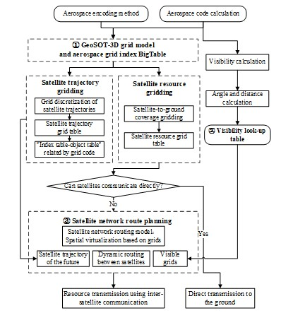
2. Methods
2.1. GeoSOT-3D and Aerospace Grid BigTable
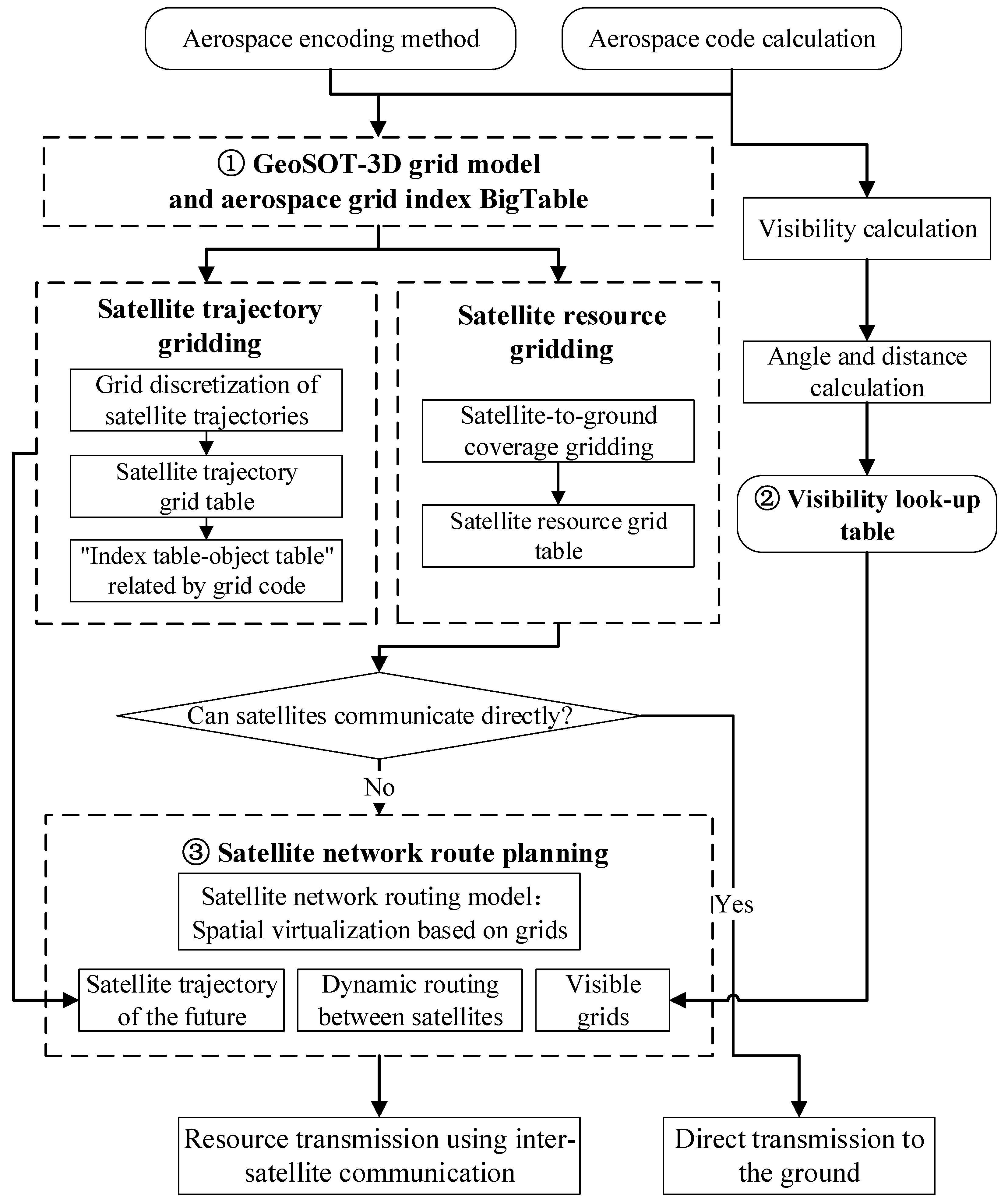
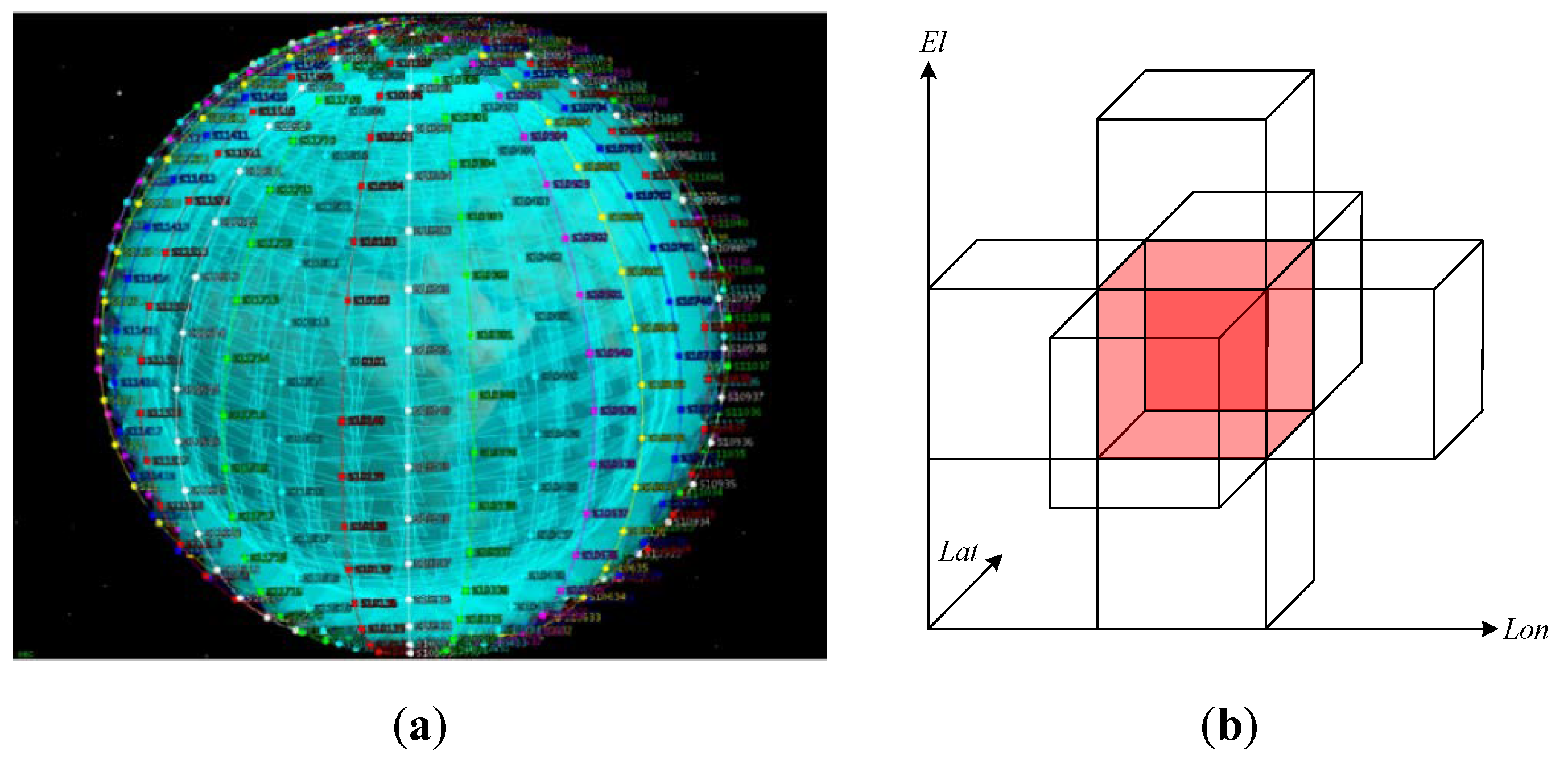
2.1.1. GeoSOT-3D Grid Model and Coding Method
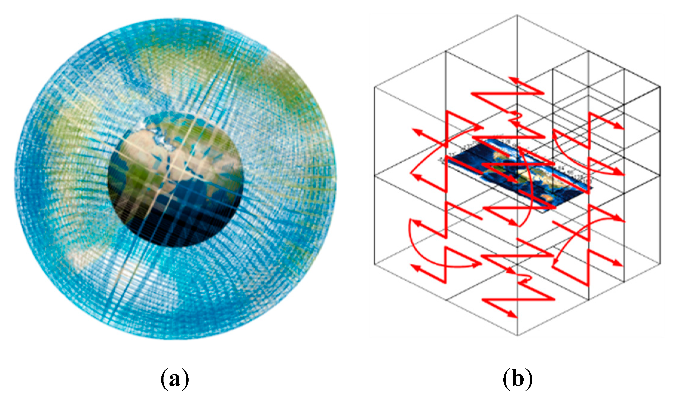
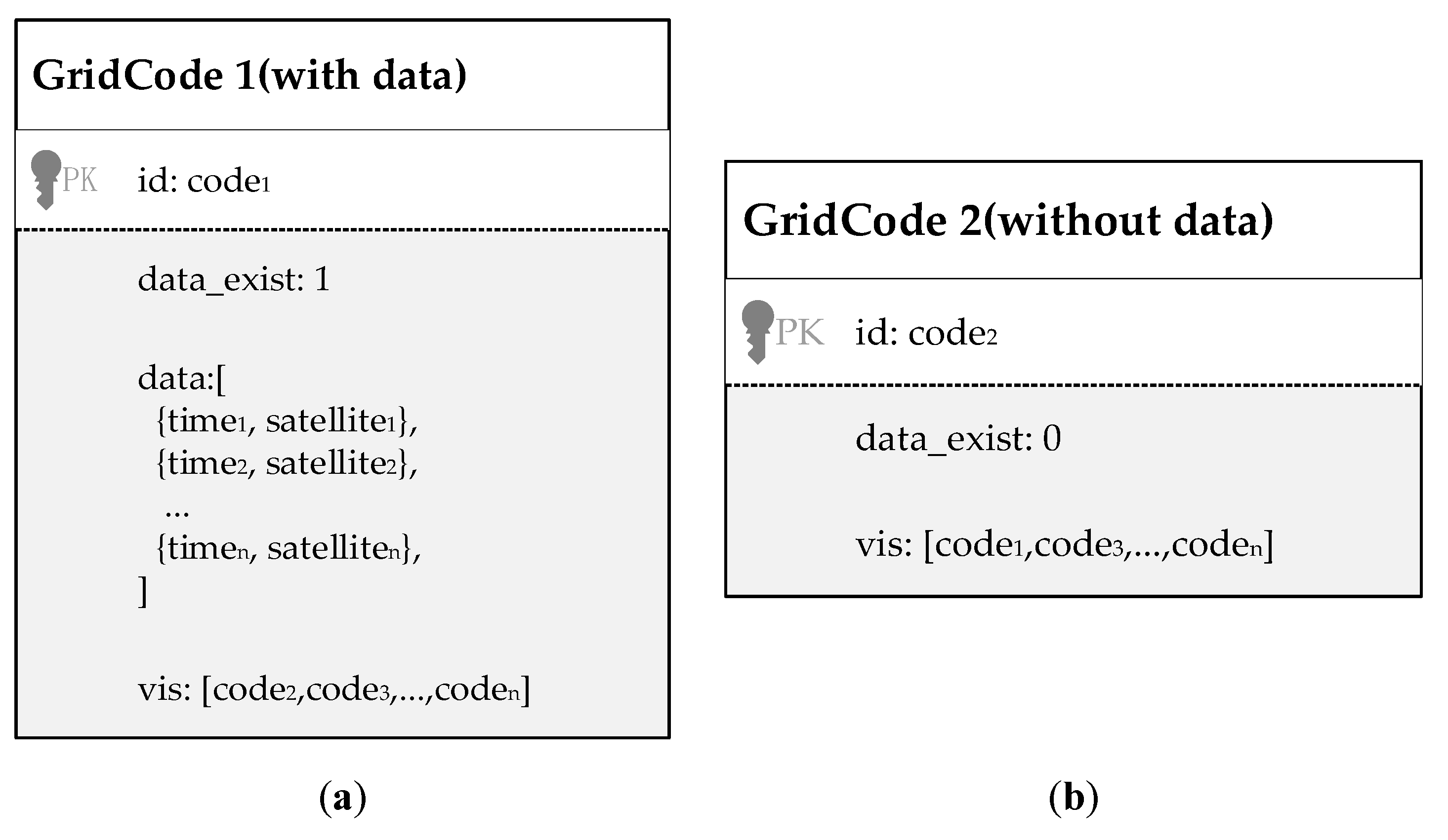
2.1.2. Aerospace Grid Indexing BigTable
2.2. Satellite Grid Visibility Algorithm
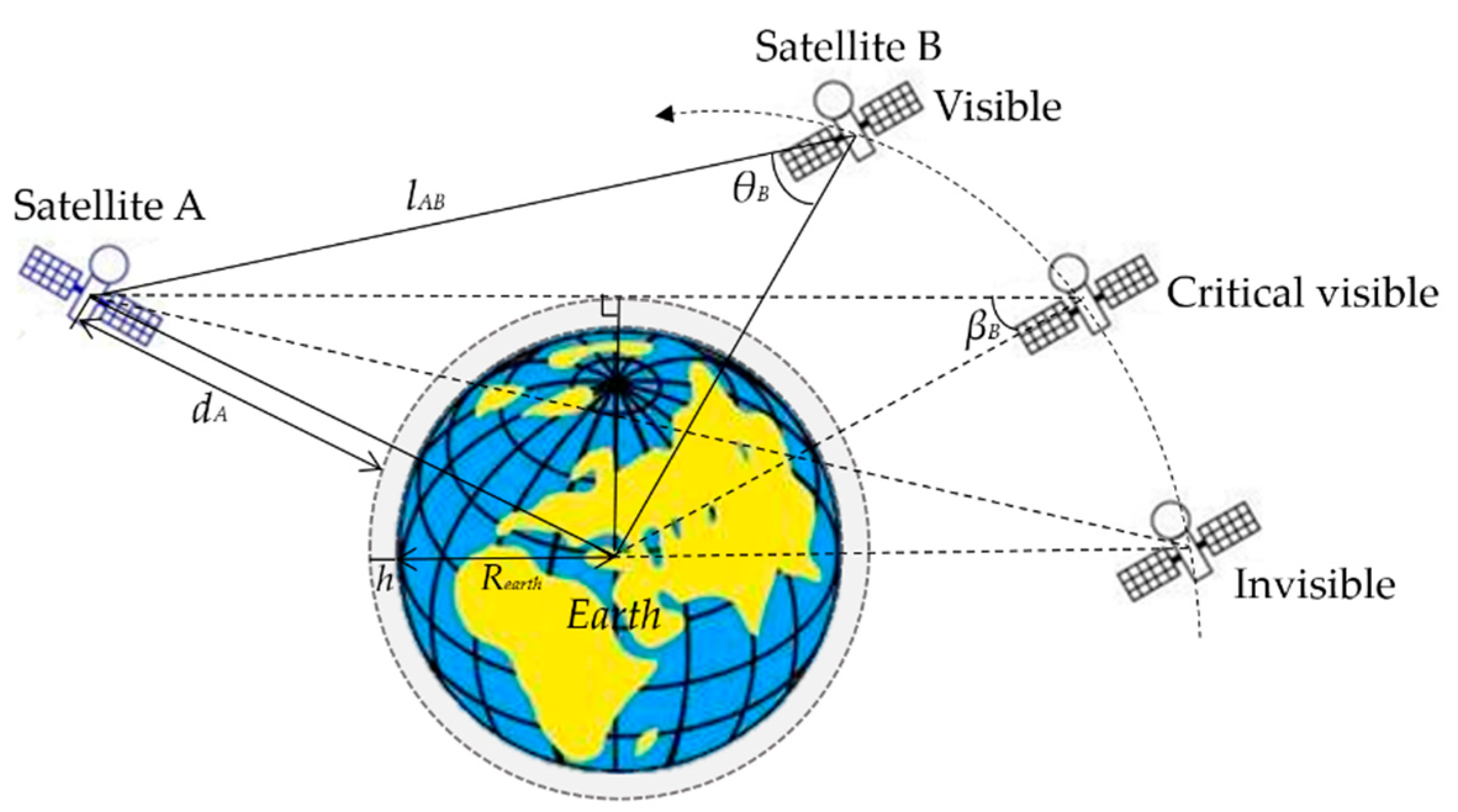
2.2.1. Traditional Satellite Visibility Analysis
2.2.2. Grid Visibility Analysis
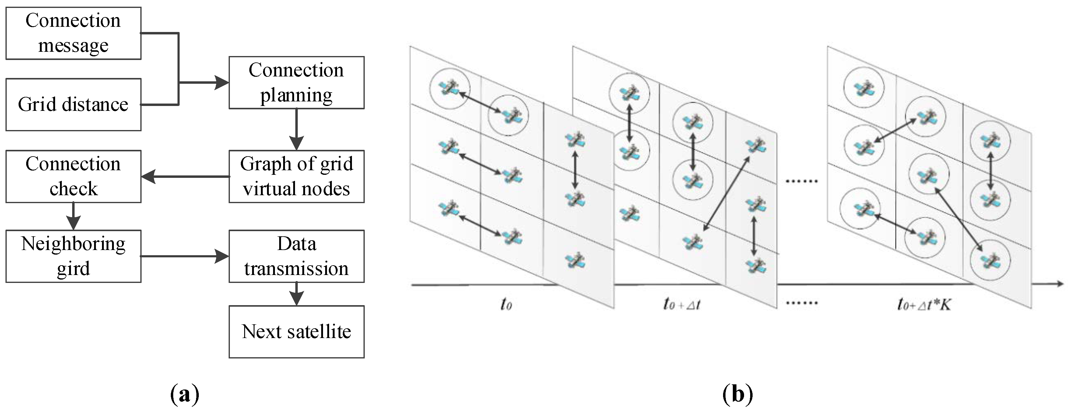
2.3. Grid Network Topology Model and Routing Algorithm
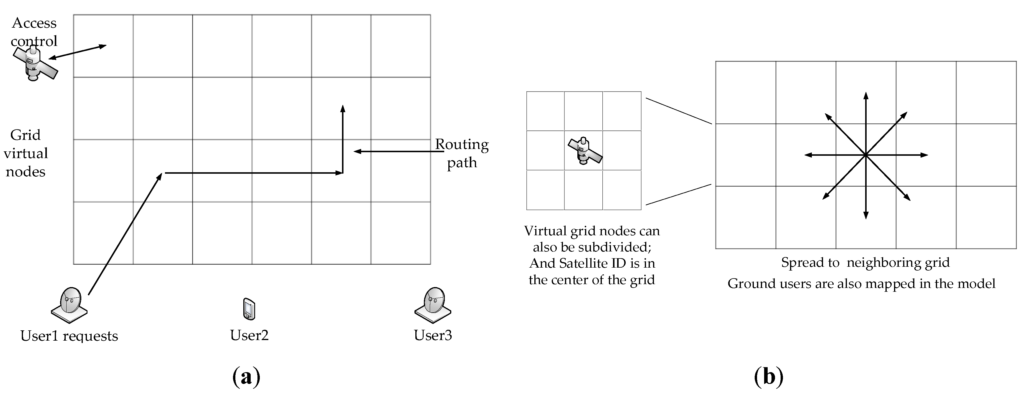
2.3.1. Grid Network Topology Model
2.3.2. Dynamic Routing Planning Algorithm
3. Experiments and Results
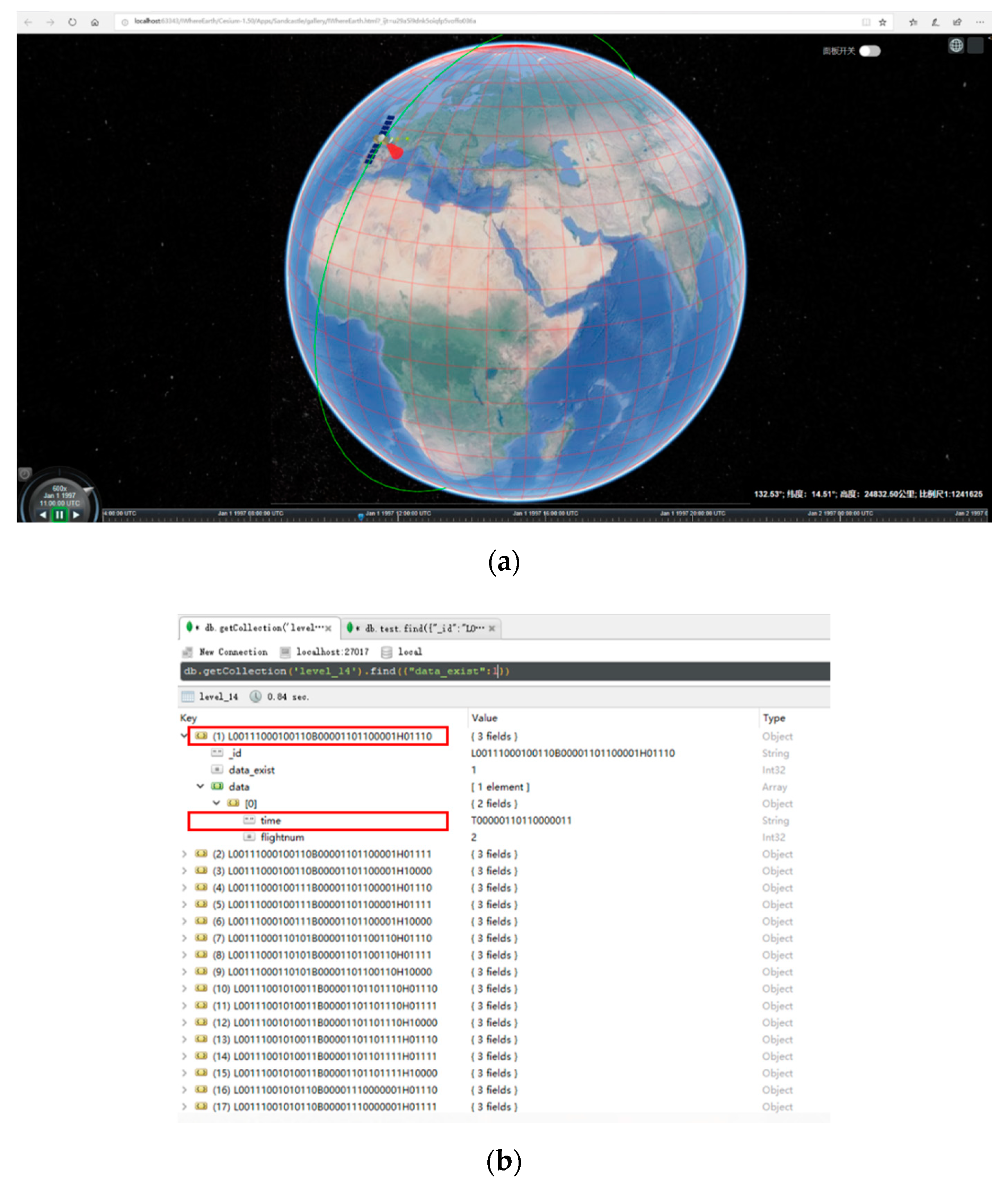
3.1. Experiment Design
3.2. Aerospace Grid Indexing BigTable
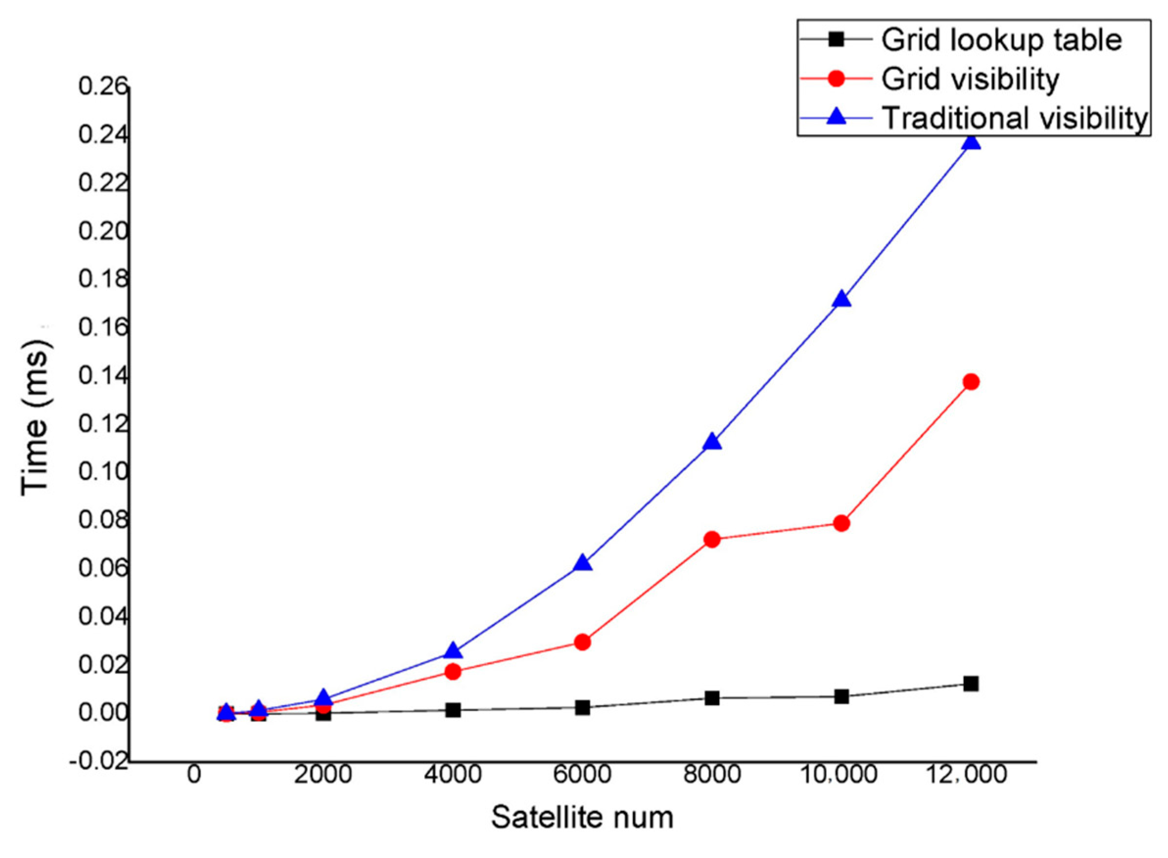
3.3. Satellite Visibility Analysis
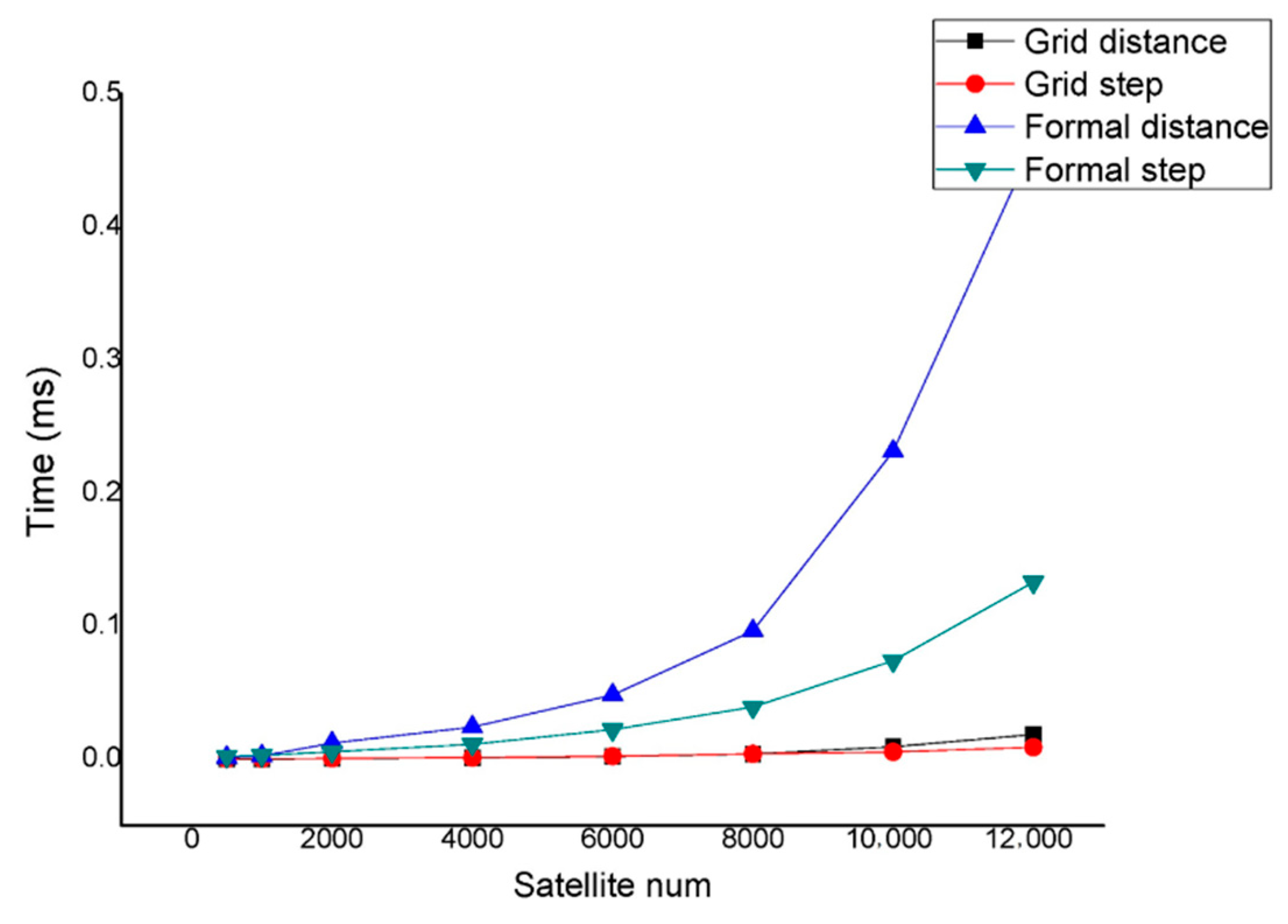
3.4. Satellite Routing Planning
4. Discussion
5. Conclusions
Author Contributions
Funding
Conflicts of Interest
References
- Sanctis, M.D.; Cianca, E.; Araniti, G.; Bisio, I.; Prasad, R. Satellite communications supporting internet of remote things. IEEE Internet Things J. 2016, 3, 113–123. [Google Scholar] [CrossRef]
- Liu, F.; Li, X.; Wang, J.; Zhang, J. An adaptive UWB/MEMS-IMU complementary Kalman filter for indoor location in NLOS environment. Remote Sens. 2019, 11, 2628. [Google Scholar] [CrossRef]
- Wei, J.; Han, J.; Cao, S. Satellite IoT edge intelligent computing: A research on architecture. Electronics 2019, 8, 1247. [Google Scholar] [CrossRef]
- Li, D.; Shen, X.; Gong, J.; Zhang, J.; Lu, J. On construction of China’s space information network. Geomat. Inf. Sci. Wuhan Univ. 2015, 40, 711–715. [Google Scholar]
- SpaceX to Launch Astronauts—And a New Era of Private Human Spaceflight. Available online: https://www.nature.com/articles/d41586-020-01554-8 (accessed on 29 May 2020).
- Mann, A. Crewed launch deepens ties between NASA and SpaceX. Science 2020, 368, 811–812. [Google Scholar] [CrossRef] [PubMed]
- Kodheli, O.; Guidotti, A.; Vanelli-Coralli, A. Integration of satellites in 5G through LEO constellations. In Proceedings of the 2017 IEEE Global Communications Conference (GLOBECOM 2017), Singapore, 4–8 December 2017; pp. 1–6. [Google Scholar]
- Chan, C.C.; Al-Hourani, A.; Choi, J.; Gomez, K.M.; Kandeepan, S. Performance modeling framework for IoT-over-satellite using shared radio spectrum. Remote Sens. 2020, 12, 1666. [Google Scholar] [CrossRef]
- Graydon, M.; Parks, L. ‘Connecting the unconnected’: A critical assessment of US satellite Internet services. Media Cult. Soc. 2020, 42, 260–276. [Google Scholar] [CrossRef]
- Liu, M.; Li, K.; Song, H.; Chen, Y.; Gao, X.; Gong, F. Using heterogeneous satellites for passive detection of moving aerial target. Remote Sens. 2020, 12, 1150. [Google Scholar] [CrossRef]
- Li, D.; Shen, X.; Li, D.; Li, S. On civil-military integrated space-based real-time information service system. Geomat. Inf. Sci. Wuhan Univ. 2017, 42, 1501–1505. [Google Scholar]
- Shimizu, K.; Ota, T.; Mizoue, N.; Saito, H. Comparison of multi-temporal PlanetScope data with Landsat 8 and Sentinel-2 data for estimating Airborne LiDAR Derived Canopy Height in Temperate forests. Remote Sens. 2020, 12, 1876. [Google Scholar] [CrossRef]
- Braten, L.E. Satellite visibility in Northern Europe based on digital maps. Int. J. Satell. Comm. 2000, 18, 47–62. [Google Scholar] [CrossRef]
- Han, S.H.; Gui, Q.M.; Li, J.W. Analysis of the connectivity and robustness of inter-satellite links in a constellation. Sci. China Phys. Mech. 2011, 54, 991–995. [Google Scholar] [CrossRef]
- Sharaf, M.A. Satellite to satellite visibility. Open Astron. 2012, 5, 26–40. [Google Scholar] [CrossRef]
- Wang, X.; Han, C.; Yang, P.; Sun, X. Onboard satellite visibility prediction using metamodeling based framework. Aerosp. Sci. Technol. 2019, 94, 1–9. [Google Scholar] [CrossRef]
- STK Access Tool. Available online: http://help.agi.com/stk/index.htm#stk/tools-01.htm (accessed on 23 May 2020).
- Tilwari, V.; Dimyati, K.; Hindia, M.N.; Mohmed Noor Izam, T.F.B.T.; Amiri, I.S. EMBLR: A high-performance optimal routing approach for D2D communications in large-scale IoT 5G network. Symmetry 2020, 12, 438. [Google Scholar] [CrossRef]
- Xia, X.; Yang, B.; Liu, Z.; An, K.; Guo, K. Performance evaluation of a full-duplex relaying-enabled satellite sensor network. Sensors 2019, 19, 5453. [Google Scholar] [CrossRef]
- Lysogor, I.; Voskov, L.; Rolich, A.; Efremov, S. Study of data transfer in a heterogeneous LoRa-Satellite network for the Internet of Remote Things. Sensors 2019, 19, 3384. [Google Scholar] [CrossRef]
- Li, X.; Zhang, X.; Ren, X.; Fritsche, M.; Wickert, J.; Schuh, H. Precise positioning with current multi-constellation Global Navigation Satellite Systems: GPS, GLONASS, Galileo and BeiDou. Sci. Rep. 2015, 5, 8328. [Google Scholar] [CrossRef]
- Sun, L.; Wang, Y.; Huang, W.; Yang, J.; Zhou, Y.; Yang, D. Inter-satellite communication and ranging link assignment for navigation satellite systems. GPS Solut. 2018, 22, 38–51. [Google Scholar] [CrossRef]
- Liu, Z.; Zhu, J.; Zhang, J.; Liu, Q. Routing algorithm design of satellite network architecture based on SDN and ICN. Int. J. Satell. Comm. Netw. 2020, 38, 1–15. [Google Scholar] [CrossRef]
- Li, J.; Ke, L.; Ye, G.; Zhang, T. Ant colony optimisation for the routing problem in the constellation network with node satellite constraint. Int. J. Bio-Inspir. Com. 2017, 10, 267–274. [Google Scholar] [CrossRef]
- Li, B.; Ge, H.; Ge, M.; Nie, L.; Shen, Y.; Schuh, H. LEO enhanced global navigation satellite system (LeGNSS) for real-time precise positioning services. Adv. Space Res. 2019, 63, 73–93. [Google Scholar] [CrossRef]
- Madni, M.A.A.; Raad, R.; Iranmanesh, S. DTN and Non-DTN routing protocols for inter-cubesat communications: A comprehensive survey. Electronics 2020, 9, 482. [Google Scholar] [CrossRef]
- Li, X.; Jiang, Z.; Ma, F.; Lv, H.; Yuan, Y.; Li, X. LEO precise orbit determination with inter-satellite links. Remote Sens. 2019, 11, 2117. [Google Scholar] [CrossRef]
- Discrete Global Grid. Available online: https://en.wikipedia.org/wiki/Discrete_global_grid (accessed on 31 May 2020).
- Tong, X.; Ben, J.; Wang, Y.; Zhang, Y. Efficient encoding and spatial operation scheme for aperture 4 hexagonal discrete global grid system. Int. J. Geogr. Inf. Sci. 2013, 27, 898–921. [Google Scholar] [CrossRef]
- Zhou, L.C.; Lian, W.J.; Zhang, Y.D.; Lin, B.X. A topology preserving gridding method for vector features in Discrete Global Grid Systems. ISPRS Int. J. Geo-Inf. 2020, 9, 168. [Google Scholar] [CrossRef]
- Cheng, C.; Tong, X.; Chen, B.; Zhai, W. A subdivision method to unify the existing latitude and longitude grids. ISPRS Int. J. Geo-Inf. 2016, 5, 161. [Google Scholar] [CrossRef]
- Li, S.; Pu, G.; Cheng, C.; Chen, B. Method for managing and querying geo-spatial data using a grid-code-array spatial index. Earth Sci. Inform. 2018, 12, 173–181. [Google Scholar] [CrossRef]
- Li, S.; Cheng, C.; Pu, G.; Chen, B. QRA-Grid: Quantitative risk analysis and grid-based pre-warning model for urban natural gas pipeline. ISPRS Int. J. Geo-Inf. 2019, 8, 122. [Google Scholar] [CrossRef]
- Miao, X.; Cheng, C.; Zhai, W.; Ren, F.; Zhang, B.; Li, S.; Zhang, J.; Zhang, H. A low-altitude flight conflict detection algorithm based on a multilevel grid spatiotemporal index. ISPRS Int. J. Geo-Inf. 2019, 8, 289. [Google Scholar] [CrossRef]
- Overview of Cloud Bigtable. Available online: https://cloud.google.com/bigtable/docs/overview (accessed on 21 June 2020).
- Park, S.; Ko, D.; Song, S. Parallel insertion and indexing method for large amount of spatiotemporal data using dynamic multilevel grid technique. Appl. Sci. 2019, 9, 4261. [Google Scholar] [CrossRef]
- Tong, X.; Cheng, C.; Wang, R.; Ding, L.; Zhang, Y.; Lai, G.; Wang, L.; Chen, B. An efficient integer coding index algorithm for multi-scale time information management. Data Knowl. Eng. 2019, 119, 123–138. [Google Scholar] [CrossRef]
- The Beauty of Bresenham’s Algorithm. Available online: http://members.chello.at/easyfilter/bresenham.html (accessed on 19 May 2020).
- Two-Line Element Set. Available online: https://en.wikipedia.org/wiki/Two-line_element_set (accessed on 19 June 2020).


| Plan of RS Satellite | Number of Satellites | Spatial Resolution | Time Resolution | Satellite Payload | Main Technical Characteristics |
|---|---|---|---|---|---|
| Planet-Dove | 140+ | 3–5 m | / | Multi-spectral | 3D observation, global coverage |
| SkySat | 24 (14) | 0.7–1 m | 6–8 h | Video/Multi-spectral | The first sub-meter optical satellite |
| BlackSky | 60 | 1 m | 10–60 min | Video/Multi-spectral | Multi-orbit constellation |
| EarthNow | 500 | Unknown | / | Unknown | Provide images and videos anywhere on the earth |
| Id | Name | Type | Description |
|---|---|---|---|
| 1 | id | STRING/INT | GeoSOT-3D grid code |
| 2 | visible | STRING/INT | Visible grid codes |
| 3 | DataExist | INT | Whether there are data in the grid (true or false) |
| 4 | Data | JSON | Data description |
| Time | TIME | Time, including the time to enter the grid, the time to leave the grid | |
| DataSource | JSON | Data source description | |
| Metadata | JSON | Metadata information |
| Query Method | Satellite Trajectory | Satellite Coverage Area | ||||
|---|---|---|---|---|---|---|
| Aera 1 | Aera 2 | Aera 3 | Aera 4 | Aera 5 | Aera 6 | |
| Lon, Lat, Height | 504.158 | 983.956 | 817.712 | 347.369 | 585.005 | 477.232 |
| GeoSOT-3D code | 53.394 | 95.743 | 87.416 | 38.03 | 85.18 | 61.47 |
| Number of Satellites | 500 | 1000 | 2000 | 4000 | 6000 | 8000 | 10,000 | 12,000 |
|---|---|---|---|---|---|---|---|---|
| Grid lookup table | 0.00001 | 0.00007 | 0.00024 | 0.00081 | 0.00171 | 0.00559 | 0.0062 | 0.01148 |
| Grid visibility | 0.00010 | 0.00072 | 0.00370 | 0.01757 | 0.02984 | 0.07247 | 0.07921 | 0.13709 |
| Traditional Visibility | 0.00014 | 0.00145 | 0.00612 | 0.02559 | 0.06208 | 0.11249 | 0.17162 | 0.23701 |
| 500 | 1000 | 2000 | 4000 | 6000 | 8000 | 10,000 | 12,000 | |
|---|---|---|---|---|---|---|---|---|
| Grid distance | 0.00005 | 0.0001 | 0.00028 | 0.00056 | 0.00153 | 0.00385 | 0.00835 | 0.0145 |
| Grid step | 0.00011 | 0.00018 | 0.00035 | 0.00051 | 0.00101 | 0.00191 | 0.00289 | 0.00547 |
| Formal distance | 0.0012 | 0.00241 | 0.01205 | 0.02209 | 0.04818 | 0.08937 | 0.23128 | 0.46256 |
| Formal step | 0.00208 | 0.00277 | 0.00554 | 0.01109 | 0.02218 | 0.03913 | 0.07392 | 0.13306 |
© 2020 by the authors. Licensee MDPI, Basel, Switzerland. This article is an open access article distributed under the terms and conditions of the Creative Commons Attribution (CC BY) license (http://creativecommons.org/licenses/by/4.0/).
Share and Cite
Li, S.; Hou, K.; Cheng, C.; Li, S.; Chen, B. A Space-Interconnection Algorithm for Satellite Constellation Based on Spatial Grid Model. Remote Sens. 2020, 12, 2131. https://doi.org/10.3390/rs12132131
Li S, Hou K, Cheng C, Li S, Chen B. A Space-Interconnection Algorithm for Satellite Constellation Based on Spatial Grid Model. Remote Sensing. 2020; 12(13):2131. https://doi.org/10.3390/rs12132131
Chicago/Turabian StyleLi, Shuang, Kaihua Hou, Chengqi Cheng, Shizhong Li, and Bo Chen. 2020. "A Space-Interconnection Algorithm for Satellite Constellation Based on Spatial Grid Model" Remote Sensing 12, no. 13: 2131. https://doi.org/10.3390/rs12132131
APA StyleLi, S., Hou, K., Cheng, C., Li, S., & Chen, B. (2020). A Space-Interconnection Algorithm for Satellite Constellation Based on Spatial Grid Model. Remote Sensing, 12(13), 2131. https://doi.org/10.3390/rs12132131