Does the Intra-Arctic Modification of Long-Range Transported Aerosol Affect the Local Radiative Budget? (A Case Study)

Abstract

The impact of aerosol spatio-temporal variability on the Arctic radiative budget is not fully constrained. This case study focuses on the intra-Arctic modification of long-range transported aerosol and its direct aerosol radiative effect (ARE). Different types of air-borne and ground-based remote sensing observations (from Lidar and sun-photometer) revealed a high tropospheric aerosol transport episode over two parts of the European Arctic in April 2018. By incorporating the derived aerosol optical and microphysical properties into a radiative transfer model, we assessed the ARE over the two locations. Our study displayed that even in neighboring Arctic upper tropospheric levels, aged aerosol was transformed due to the interplay of removal processes (nucleation scavenging and dry deposition) and alteration of the aerosol source regions (northeast Asia and north Europe). Along the intra-Arctic transport, the coarse aerosol mode was depleted and the visible wavelength Lidar ratio (LR) increased significantly (from 15 to 64–82 sr). However, the aerosol modifications were not reflected on the ARE. More specifically, the short-wave (SW) atmospheric column ARE amounted to +4.4 - +4.9 W m⁻² over the ice-covered Fram Strait and +4.5 W m⁻² over the snow-covered Ny-Ålesund. Over both locations, top-of-atmosphere (TOA) warming was accompanied by surface cooling. These similarities can be attributed to the predominant accumulation mode, which drives the SW radiative budget, as well as to the similar layer altitude, solar geometry, and surface albedo conditions over both locations. However, in the context of retreating sea ice, the ARE may change even along individual transport episodes due to the ice albedo feedback.

1. Introduction

As anthropogenic climate change drives major modifications in the Arctic environment, Arctic aerosol and its related feedback mechanisms are inextricably affected. Aerosol is involved in aerosol–cloud and aerosol–radiation interactions, which highly depend on the aerosol species, solar zenith angle, and surface albedo [1,2,3]. In the Arctic, the annual mean aerosol radiative forcing at the top-of-atmosphere (TOA) is estimated at −0.12 W m⁻² with respect to pre-industrial emissions of anthropogenic aerosol and precursors [3]. Over the past century, the aerosol-induced cooling has offset the greenhouse gas-induced warming by 1.3 to 2.2 °C [4]. However, the aerosol radiative forcing in the Arctic region still entails high uncertainties [1,2,3]. Therefore, a better understanding of the aerosol-related physical processes is crucial in the changing Arctic environment, where the most rapid near-surface temperature increase is taking place, known as “Arctic amplification” [5,6].

Arctic aerosol properties exhibit a pronounced seasonal cycle due to variation in sources, transport pathways, and removal processes [7,8,9,10]. On a pan-Arctic scale, the accumulation mode concentration increases through winter and peaks in April, with median values between 100 and 200 cm⁻³ [11,12,13]. This seasonality is reflected upon the aerosol optical properties, with a late winter–spring scattering coefficient maximization (median values even higher than 10 Mm⁻¹) [10]. While in winter, maximal extinction occurs in the lower Arctic troposphere, in spring, there is a progressive shift towards the middle and upper troposphere [13,14,15]. The extinction enhancement in higher altitudes (“Arctic haze”) is associated with the isentropic poleward transport of polluted mid-latitude air masses [16,17,18]. “Arctic haze” comprises mostly aged accumulation particles of sulfate composition. However, chemical analysis has illustrated the presence of nitrate, chloride, sea salt, ammonium, dust, and carbonaceous compounds [14,19,20,21,22]. Studies have also demonstrated contribution from biomass-burning sources [12,23,24,25,26,27].

Ny-Ålesund (78.9°N, 11.9°E), Spitsbergen island, Svalbard is an Arctic research site embedded in a complex orography of fjord and mountain ranges. The Svalbard region is the hotspot of winter warming with up to 2 °C per decade near-surface temperature increase in the past two decades [28] and a 5–20% decadal decrease in fjord sea ice coverage [29]. One quarter of this warming is attributed to the amplified advection of warm and moist air-masses over the mid-latitude Atlantic Ocean, which is facilitated by changes in large-scale circulation, such as atmospheric blocking patterns [30,31]. In the context of enhanced local humidity fluxes from the increasingly ice-free Arctic Ocean, the springtime AOD over Ny-Ålesund has diminished over the past two decades [32].

Despite the overall distinct annual patterns, the seasonal cycle of aerosol properties presents consistent discrepancies within the Arctic. Synergistic ground-based and air-borne aerosol observations can provide insight into intra-Arctic aerosol modification and improve its representation into chemical transport and climate models. Lidar systems are key observational tools of aerosol, with the asset of delivering vertically resolved measurements on high spatial and temporal scales [33]. Moreover, the Raman Lidar technique delivers a suite of optical parameters from which the aerosol microphysical properties can be inferred [34,35,36,37], allowing the evaluation of aerosol radiative effects.

Our study focused on a persistent aerosol transport episode, which was synergistically identified by remote sensing systems in remarkably high tropospheric altitudes. The elevated aerosol layers were revealed over two parts of the European Arctic, namely Fram Strait and Ny-Ålesund, three days apart in April 2018 (Figure 1 and Figure 2). Our primary target was to investigate the intra-Arctic modification of the aerosol optical and microphysical properties. By incorporating the derived aerosol properties into a radiative transfer model, we aimed to assess the direct aerosol radiative effect (ARE) and quantify the related uncertainties.

2. Methods: Instrumentation and Modeling Tools

In this study, we utilized active and passive remote sensing observations over two parts of the European Arctic in order to retrieve the optical and microphysical properties of long-range transported aerosol. The ensemble of inverted aerosol properties was incorporated into a radiative transfer model to assess the ARE and its related uncertainties. In parallel, the simulated irradiances were evaluated with ground-based and air-borne observations.

2.1. Lidar Systems

The elastic air-borne mobile aerosol Lidar (AMALi) is installed on board of the research aircraft Polar 5 [38]. During the polar air-borne measurements and Arctic Regional Climate Model Simulation Project 2018 (PAMARCMiP2018), AMALi was operated in zenith configuration during 9 flights (25 March–4 April for approximately 32 h in total) over the region of Fram Strait (84, 17 NW to 79, 20 NE). AMALi is equipped with an Nd:YAG laser that emits pulses at 15 Hz. A 10-cm off-axis telescope mirror of 3.1 mrad field of view (FOV) collects the backscattered light. Photomultiplier tubes (PMTs) are used for the detection of elastically backscattered photons at 532 and 355 nm. Additionally, the cross-polarized component is recorded at 532 nm, allowing for the determination of the aerosol linear depolarization ratio, hereafter mentioned as the aerosol depolarization ratio.

AMALi signal returns were acquired with a 1 s––7.5 m resolution. Signals were vertically averaged every 30 m and smoothed with a 90-m window, while backscatter profiles were smoothed with a 150-m window. The altitude of the observed features was corrected with respect to the aircraft movements, with the pitch and roll angles changing by 2° and 3.5° during the evaluation windows. For this study, we extracted two observation periods of a 2- and 5-min duration (as indicated in Figure 1 and Figure 2a), which were limited by the changing flight altitude. The signal-to-noise ratio (SNR) changed considerably due to the variable flight altitude (0.3–2.9 km) during AMALi observations, which limited the temporal averaging and led to higher uncertainties in the air-borne-derived optical properties compared to the ground-based ones.

The multi-wavelength Koldewey Aerosol Raman Lidar (KARL) is operated in the Alfred Wegener Institute Emille Victor (AWIPEV) research base, Ny-Ålesund, Svalbard. KARL is a “3β+2α+2δ+2wv” system equipped with an Nd:YAG laser emitting at 1064, 532, and 355 nm after frequency doubling and tripling, respectively [39]. The pulse repetition rate of the system is 50 Hz, emitting approximately 10 W in each wavelength. The receiver consists of a parabolic 70 cm diameter Newtonian telescope with a 1.75 mrad FOV and an aperture with an adaptable position and pinhole diameter. PMTs are used for the detection of backscattered photons in all channels, except for 1064 nm, where avalanche photodiodes (APDs) are used. KARL signal returns were obtained with a 1.5 min-7.5 m resolution. In order to reduce signal noise, we averaged the profiles for approximately 2.5 h and applied vertical smoothing of 157.5 m in the backscatter retrieval and 225 m in extinction retrieval, following the effective resolution concept [40].

We applied the Klett–Fernald method to the elastic AMALi and KARL signals in order to retrieve the backscatter profiles [41,42]. This method requires a priori information on the vertical profile of the extinction-to-backscatter ratio (Lidar ratio or LR) and a reference value for the backscatter ratio (total backscatter over molecular backscatter). Here, we assumed uncertainties of 10 sr and 3% for the LR and backscatter ratio, respectively. The positioning of the calibration window introduces additional uncertainty. Errors are also introduced due to statistical signal noise and the procedures of temporal averaging and vertical smoothing. We obtained extinction profiles from KARL by utilizing the Raman method [43]. Since Raman scattering cross-sections are orders of magnitude lower than Rayleigh cross-sections and our observations were performed during the Polar day period, we derived layer-mean values of extinction and LR. Aerosol optical properties are presented in

Table 1. Aerosol optical properties (mean ± one standard deviation) over two parts of Fram Strait and Ny-Ålesund retrieved from AMALi and KARL, respectively. For details on the retrieval procedure, see Section 2.1. The aerosol backscatter coefficient β, backscatter-related Angström exponent A_β, and aerosol depolarization ratio δ are presented.

Aerosol Optical Properties
Aerosol Properties	Fram Strait (AMALi)		Ny-Ålesund (KARL)
	2 April		5 April		6 April
	10:31–10:33	12:04–12:09	11:00–13:47		9:51–10:41
aerosol layer altitude (km)	5.15–6.8	5.3–6.9	4.3–4.9	4.9–5.75	4.6–5
${\beta }_{355}^{aer}$ (Mm−1sr−1)	1.3 ± 0.3	1.7 ± 0.5	0.5 ± 0.1	0.6 ± 0.1	1 ± 0.3
${\beta }_{532}^{aer}$ (Mm−1sr−1)	0.9 ± 0.1	1 ± 0.2	0.2 ± 0.05	0.3 ± 0.06	0.4 ± 0.2
${\beta }_{1064}^{aer}$ (Mm−1sr−1)	-	-	0.1 ± 0.03	0.1 ± 0.03	0.2 ± 0.1
${\mathrm{\AA }}_{\beta 355/\beta 532}$	0.8 ± 0.6	1.3 ± 0.4	1.8 ± 0.2	2.2 ± 0.1	2.4 ± 0.3
${\mathrm{\AA }}_{\beta 532/\beta 1064}$	-	-	1 ± 0.1	1.1 ± 0.04	1.2 ± 0.3
${\delta }_{355}^{aer}$ (%)	-	-	3.8 ± 0.6	2.9 ± 0.3	3.9 ± 0.8
${\delta }_{532}^{aer}$ (%)	1.3 ± 0.2	5.5 ± 1	3.2 ± 0.3	3 ± 0.2	3.4 ± 0.4

and

Table 2. Aerosol layer mean optical properties over the Greenland side of Fram Strait retrieved from the synergy of sun-photometer and KARL and over Ny-Ålesund as derived from KARL. The aerosol extinction coefficient α, Lidar ratio LR, and extinction-related Angström exponent A_α are presented. Values estimated by Mie theory are given in italic. For details, see Section 2.1 and Section 2.2. The extinction over Fram Strait was estimated by Equation (2).

Aerosol Layer-mean Optical Properties
Aerosol Properties	Fram Strait (Sun-photometer and KARL)	Ny-Ålesund (KARL)
	2 April	5 April
	10:52–10:57	11:00–13:47
aerosol layer altitude (km)	5.15–6.8	4.3–4.9	4.9–5.75
$a_{355}^{aer}$ (Mm−1)	-	18 ± 7	30 ± 8
$a_{496}^{aer}$ (Mm−1)	20 ± 2	-	-
$a_{532}^{aer}$ (Mm−1)	21 ± 2	20 ± 5	16 ± 6
$a_{675}^{aer}$ (Mm−1)	27 ± 1	12 ± 2	12 ± 2
$a_{779}^{aer}$ (Mm−1)	28 ± 1	10 ± 2	9 ± 2
$a_{861}^{aer}$ (Mm−1)	25 ± 1	9 ± 2	7 ± 2
$a_{1026}^{aer}$ (Mm−1)	20 ± 1	7 ± 2	4 ± 2
LR355 (sr)	-	35 ± 15	48 ± 4
LR532 (sr)	15 ± 3	82 ± 25	64 ± 37
${\mathrm{\AA }}_{a355/a532}$	-	−0.3 ± 0.8	1.5 ± 1.8
Åα496-α1026	−0.09	-	-

.

2.2. Sun-Photometers and Extinction Estimation at Fram Strait

The air-borne Sun-photometer with an active tracking system (SPTA) was operated under a quartz dome on the top of Polar 5 during PAMARCMiP2018. The aerosol optical depth (AOD) was provided at 10 wavelengths between 396 and 1026 nm every 30 sec. Unfortunately, the 369–414 nm channels presented calibration issues and, thus, they were not used for further evaluation. Moreover, we did not use the 946-nm channel, which is dedicated to water vapor (WV) absorption. On 2 April, the AOD was measured at different flight levels between 0.04 and 5.15 km (Figure 3). We performed 5-min averaging in the AOD in order to reduce statistical noise. The aerosol extinction coefficient was estimated by consecutive AOD pairs within altitude layers of 0.5–2.2 km and temporal periods of 5–40 min, within which the atmospheric conditions were assumed to be horizontally homogeneous (similar AOD at similar altitudes, Figure 3).

The AOD of the elevated aerosol layer (5.15–6.8 km), observed close to the Greenland side of Fram Strait (Figure 1 and Figure 2a), was estimated by combining photometer and Lidar observations. More specifically, we used the photometer AOD at five different measurement points below the layer, between the highest photometer observation (number 5, 10:52–10:57 UT; flight level 5.15 km) and the closest AMALi observation (number 1, 10:31–10:33 UT; flight level 2.8 km). We also used the AOD at three intermediate flight levels (numbers 2, 3, and 4 corresponding to 3, 4.3, and 4.4 km) so as to better constrain the estimated extinction. The AOD was calculated according to Equation (1), with the selected measurement points enumerated in Figure 3. Horizontal homogeneity was assumed due to the short spatial (maximum 100 km) and temporal differences (maximum 25 min) among the measurement points, as in the study of Mei et al. [44] that focused on satellite aerosol remote sensing. Above the aerosol layer, the AOD was derived from KARL. The ground-based Lidar signals were preferred over the air-borne ones due to their higher SNR. The aerosol load in the stratosphere was invariable between the air-borne and ground-based observations (three days and a maximum of 500 km apart). The AOD was the product of the integrated backscatter with the LR. The KARL AOD was interpolated to the photometer wavelengths using an appropriate Angström exponent (1.8 as fitted to the backscatter at 355, 532, and 1064 nm). Following the same steps, we estimated the stratospheric AOD. Finally, the extinction of the elevated aerosol layer was estimated by Equation (2):

$$AO{D}_{5.15-6.8km}=AO{D}_{2.8km}^{sun-photometer}-AO{D}_{3-4.3km}^{sun-photometer}-AO{D}_{4.4-5.15km}^{sun-photometer}-AO{D}_{6.8km-tropopause}^{KARL}-AO{D}_{stratosphere}^{KARL}$$

(1)

$$a_{5.15-6.8km}=\frac{AO{D}_{5.15-6.8km}}{Layergeometricaldepth}.$$

(2)

Over Ny-Ålesund the AOD was measured by an SP1a type sun-photometer in 10 wavelengths between 369 and 1023 nm. A cloud screening procedure that relies on the short-term AOD variability was applied to the data [45]. The total AOD uncertainty amounted to 0.01 [32]. In this study, we only utilized the wavelengths, which are spectrally closer to the air-borne photometer channels, except for the 1023 nm that was affected by calibration issues.

2.3. Aerosol Microphysical Properties Inversion Schemes

We incorporated the set of optical parameters derived for Fram Strait and Ny-Ålesund into inversion algorithms so as to retrieve the aerosol microphysical properties. In the inversion schemes, the extinction and backscatter coefficients were used as input for the derivation of the complex refractive index and aerosol volume size distribution using Mie theory. For each combination of the real and imaginary refractive index, the best solution was identified. More specifically, the least residuum between the backward (input) and forward calculated optical parameters was selected. The standard deviation of the best solutions represents the uncertainties of the complex refractive index. Statistical noise and systematic uncertainties of the input optical parameters together with mathematical approximation errors contribute additively to the total uncertainties in the microphysical parameters.

For Fram Strait, we utilized the AMALi-derived backscatter coefficient (355 and 532 nm) together with the sun-photometer-derived extinction (496, 675, 779, 861, and 1026 nm). We employed collocation discretization and an iterative Padé-regularization method with a fixed number of 30 iterations [35,36]. For Ny-Ålesund, the KARL-derived aerosol backscatter (355, 532 and 1064 nm) and extinction coefficients (355 and 532 nm) were inverted to the particle microphysics employing a truncated singular value decomposition regularization algorithm [34]. More details about the Lidar inversion algorithms, which have been developed at the University of Potsdam, can be found in [34,37,46].

The total number (n_t), surface-area (s_t), and volume (v_t) concentration, as well as the effective radius (r_eff) were derived for the fine and coarse aerosol modes by performing log-normal fits to the inverted volume distribution. Fitting errors amounted to 10% for the total concentrations and 5% for the r_eff estimation. The single-scattering albedo (SSA) and the asymmetry parameter were calculated from the fitted number size distributions utilizing Mie theory. The corresponding SSA and asymmetry parameter uncertainties were estimated by sensitivities based on different complex refractive index scenarios.

2.4. Trajectory Calculations for Air-Mass History

In order to assay the origin of the observed transport event and link the evolution of aerosol properties with intruding air masses, we performed 10-day LAGRANTO backward trajectories over Fram Strait and Ny-Ålesund [47,48]. A significant number of trajectories ending over Fram Strait and Ny-Ålesund originated from the lower troposphere, providing an indication for the surface aerosol sources. Due to the complex orography of Spitsbergen island, with the highest peak at 1.7 km, and the challenging to parameterize stable boundary layer, we are inclined to have higher confidence in higher altitude trajectories.

We used ECMWF analysis data to calculate trajectories with LAGRANTO, which utilizes the three-dimensional wind field to calculate kinematic trajectories. The ECMWF data for this study had a horizontal grid spacing of 0.5° x 0.5° with 137 hybrid sigma pressure levels in total. Analysis fields were available every six hours. For the flight locations over Fram Strait, we initialized the trajectories in a small region around the flight track. Trajectories from Ny-Ålesund were initialized every 0.05° in the horizontal within a 0.5° × 0.5° box centered at Ny-Ålesund. Trajectory information was then available every hour. Ancillary meteorological parameters, such as pressure and relative humidity (RH), were calculated along the trajectories. The spatial variability of the trajectories was taken into account by using a box, instead of a single point, for initializing our calculations. Moreover, the influence of atmospheric variability was considered by analyzing coherent bundles of trajectories instead of single trajectories.

2.5. Radiation and Meteorological Observations

We utilized air-borne and ground-based irradiance observations for evaluating the modeled irradiances at the surface and different flight altitudes. Radiation sensors were installed on the top and bottom of the Polar 5 fuselage during PAMARCMiP2018. More specifically, a CMP22 Pyranometer by Kipp&Zonen was measuring broadband (0.2–3.6 μm) global and reflected solar irradiances. The measurement repetition rate was 20 Hz, with all the irradiances being deconvoluted for their inertia time [49]. The overall uncertainty was lower than 10 W m⁻² for all radiation quantities. Basic meteorological observations were also performed on board of the Polar 5 aircraft [50]. WV concentration was measured by the LI-7200 closed CO₂/H₂O analyzer [51].

At Ny-Ålesund, radiation measurements are performed within the frame of the Baseline Surface Radiation Network (BSRN) since 1992 [52]. Short-wave (SW) broadband radiation in the range 0.2 to 3.6 μm is measured with CMP22 pyranometers by Kipp&Zonen, installed in an up- and downward orientation for global and reflected radiation, respectively. In addition, the diffuse radiation is obtained by ball-shaded similar instrumentation. The basic surface radiation and meteorological measurements with a one-minute resolution applied in our study are available via the Pangaea data repository [53]. Vertical profiles of the temperature, RH, wind speed, and direction in the upper atmosphere are applied from daily radiosonde ascents performed at the AWIPEV station [54].

2.6. Radiative Transfer Simulations

In order to quantify the altitude-dependent direct ARE and its uncertainties, we performed simulations with the radiative transfer model SCIATRAN [55], using as input the retrieved aerosol optical and microphysical properties. For the evaluation of the simulated irradiances, the latter were integrated within the spectral range of the BSRN and air-borne pyranometers.

We performed simulations from the local surface up to 40 km. The vertical resolution varied from 50 m to 1 km (above 10 km). The radiative transfer equation was solved by means of the scalar discrete ordinate technique, while a plane-parallel atmosphere approximation was used. The absorption contribution of line absorbers was computed in line-by-line mode of 0.01-nm spectral resolution, based on the spectroscopic parameters of the HITRAN 2008 database [56]. The altitude-dependent ARE was derived from the difference of SW net irradiances between the respective aerosol and the off-aerosol scenario, in order to distinguish it from the total atmospheric effect. The difference between the TOA and surface ARE yielded the overall atmospheric column ARE.

The aerosol-related input comprised the spectrally resolved aerosol extinction coefficient (Table 2), the SSA, as well as the asymmetry factor calculated according to the Henyey–Greenstein parameterization (

Table 3. Aerosol microphysical properties over the Greenland side of Fram Strait and Ny-Ålesund. The complex refractive index ri, the single-scattering albedo SSA, and the asymmetry parameter g are given. Moreover, the effective radius r_eff as well as the number n_t, surface s_t, and volume v_t concentrations are presented for the fine and coarse aerosol modes. For details on the retrieval schemes, see Section 2.3.

Aerosol Microphysical Properties
Aerosol Properties	Fram Strait (AMALi and Sun-Photometer)		Ny-Ålesund (KARL)
	2 April		5 April
	10:31–10:57		11:00–13:47
aerosol layer altitude (km)	5.15–6.8		4.3–4.9		4.9–5.75
Refractive Index ri (mean ± one standard deviation)
ri	1.5 + 0.008 i ± 0.02 + 0.006 i		1.54 + 0.019 i ± 0.04 + 0.01 i		1.49 + 0.007 i ± 0.02 + 0.004 i
Single-Scattering Albedo SSA (mean ± uncertainty)
SSA355 SSA532	0.84 ± 0.1 0.91 ± 0.06		0.88 ± 0.06 0.9 ± 0.05		0.96 ± 0.02 0.96 ± 0.02
Asymmetry parameter g (mean ± uncertainty)
g355 g532	0.69 ± 0.04 0.7 ± 0.05		0.71 ± 0.04 0.69 ± 0.03		0.72 ± 0.02 0.68 ± 0.01
Effective radius reff, number nt, surface st and volume vt concentration
	fine	coarse	fine	coarse	fine	coarse
reff (μm)	0.49	1.26	0.26	1.43	0.19	-
nt (cm−3)	8.78	0.24	65.2	0.005	132.9	-
st (μm2 cm−3)	24.09	4.68	21.6	0.13	36.4	-
vt (μm3 cm−3)	3.9	1.97	1.9	0.06	2.3	-

). The aerosol optical and microphysical properties were extrapolated to the model’s spectral range (from 355–1026 nm) by forward Mie theory. More specifically, using the aerosol refractive index and number size distribution as input, we were able to calculate the aerosol extinction coefficient at any wavelength. The surface albedo over Fram Strait and Ny-Ålesund was obtained from air-borne and BSRN pyranometer observations, respectively. A surface albedo of approximately 0.7 was found for both locations, revealing the presence of sea ice at Fram Strait and snow-covered tundra in Ny-Ålesund.

For Fram Strait, we performed four simulation scenarios: Aerosol and off-aerosol for the aircraft positions during the AMALi and sun-photometer evaluation periods, as indicated in Figure 1. Thermodynamic profiles were constructed as a combination of appropriately selected air-borne meteorological observations below 5 km (pressure and temperature from aircraft meteorological observations, WV mixing ratio from LI-7200 instrument) and radiosonde ascents from Ny-Ålesund aloft (approximately 500 km distance from flight operations). Between 5 and 8 km, a hybrid air-borne – radiosonde profile was constructed, which gradually shifted from the highest air-borne towards the radiosonde observations.

For Ny-Ålesund, simulations were performed for the period of available Raman Lidar observations (5 April, 11:00–13:30). The simulations comprised four different scenarios: Off-aerosol, with two aerosol layers (4.3–5.75 km), with the lower layer (4.3–4.9 km) and finally with the upper layer (4.9–5.75 km). Ancillary meteorological information on the temperature at the surface, 2 and 10 m, as well as surface pressure, were also incorporated into the model. Pressure, temperature, WV mixing ratio, and O₃ concentration profiles were taken from a collocated ozonesonde ascent (5 April, AWIPEV). For both Arctic locations, further trace gas profiles were obtained from climatological profiles for the given month and latitude [57].

3. Aerosol Observations over the European Arctic and Meteorological Conditions

Air-borne observations were performed within the frame of PAMARCMiP2018 (March-April), Villum Research Station, Greenland (81.6°N, 16.7°W). The PAMARCMiP2018 period was characterized by a high-pressure system over the North Pole, while some weak lows occurred over northeast Greenland. On 2 April, a well-defined aerosol layer was identified at a remarkably high tropospheric altitude over Fram Strait by AMALi and sun-photometer (Figure 1 and Figure 2a). Three days later, a geometrically similar aerosol layer was observed by KARL over Ny-Ålesund (Figure 2b), at a distance of 200–600 km from the flight operations. In the interim of Fram Strait and Ny-Ålesund on 3 April, clouds and aerosol remnants were captured in the upper troposphere by AMALi (Figure S1). At that day, Raman Lidar observations over Ny-Ålesund were not allowable due to low-level clouds. However, the micro-pulse Lidar (MPL, technical description given in Shibata et al. [18]) provided the geometrical evolution of the aerosol layers. It should be noted that the MPL optical products cannot be utilized for the derivation of aerosol microphysical properties due to the lack of Raman channels. Therefore, the optical and microphysical aerosol properties over Ny-Ålesund were investigated within periods of 5 and 6 April as indicated in Figure 2b. On the days when the aerosol layer was observed over Ny-Ålesund, the synoptic situation was characterized by the passing of a weak low-pressure system. According to radiosonde ascents from Ny-Ålesund, moderate N-NW winds (3–7 m/s) prevailed, while wind shear and RH were enhanced (RH of 47– 58% on 5 April and 55–65% on 6 April) at the aerosol layer atmospheric levels.

4. Results

4.1. Episode Evolution over Ny-Ålesund and Connection to Air Masses

The geometrical evolution of the transported aerosol plume over Ny-Ålesund along with the related air mass trajectories are presented in Figure 4. The columnar AOD over Ny-Ålesund and Fram Strait are demonstrated in Figure 5. Before the layer arrival (30–31 March), air masses originated from central Eurasia (4–7 km, Figure 4b). The daily mean AOD₅₀₀ was relatively low (0.04 ± 0.01) with respect to background values (AOD₅₀₀ = 0.06 from Yamanouchi et al. [58]). The influence of northeast Asian air masses is discernible for 2 April, with aerosol features appearing entangled with clouds. Due to persistent low-level clouds (2–4 April), Raman Lidar and sun-photometer observations were unfortunately not allowable during those days.

On 5 April, the layer displayed a well-defined structure. The AOD₅₀₀ followed a moderate increasing tendency with persisting northeast Asian and emerging north European air masses (Figure 4d). On 6 April, the layer was vertically perturbed (Figure 4c,6 April 0-8 UT), possibly due to the passing of the weak low-pressure system. The AOD₅₀₀ fluctuated and maximized (AOD₅₀₀ = 0.13) some hours later. The layer gradually diluted (7 April), with the AOD approaching background levels. Re-emerging low-level clouds did not allow us to further investigate the event evolution, with intermittent aerosol features and mid-level clouds mostly observed (8 April). Overall, the AOD over Ny-Ålesund was clearly lower compared to Fram Strait. In Section 4.3 and Section 4.4, we will investigate in more detail the modification of aerosol optical and microphysical properties within the elevated aerosol plume.

4.2. Origin of Observed Aerosol Over Fram Strait and Ny-Ålesund

Prior to investigating the modification of aerosol optical and microphysical properties, we assessed whether the observed aerosol plumes over Fram Strait and Ny-Ålesund originated from the same region or regions comprising similar aerosol sources. The atmospheric pressure along the LAGRANTO backward trajectories as well as the air mass transport time are displayed in Figure 6.

At Fram Strait, the layer close to Greenland (Figure 6a) was a receptor of central and northeast Asian air masses, which were at least nine days old (time since contact with main aerosol source region, Figure 6c). At Ny-Ålesund, the lower part of the plume originated from north Europe (Figure 6d), while the upper part was also affected by northeast Asian air masses (Figure 6e). On their arrival at Ny-Ålesund, the Asian air masses were at least nine days old, while the north European ones had last contact with the main aerosol sources four days ago (Figure 6f). The latter air masses mixed over Fram Strait (500–600 hPa) in the earlier days (Figure 6f).

4.3. Modification of Aerosol Optical Properties

The optical properties of the long-range transported aerosol over Fram Strait and Ny-Ålesund are summarized in Table 1 and Table 2, for the evaluation periods indicated in Figure 1 and Figure 2. The vertical profiles of the aerosol backscatter coefficient (proportional to the aerosol number concentration), aerosol depolarization ratio (rising with aerosol non-sphericity), and backscatter-related Angström exponent (inversely proportional to aerosol radius) are demonstrated in Figure 7. The aerosol extinction coefficient and extinction-related Angström exponent as derived by sun-photometer and Lidar are presented in Figure 8.

A shift towards smaller particles was observed, mainly between Fram Strait and Ny-Ålesund, as well as between 5 and 6 April over Ny-Ålesund. Over Fram Strait, the layers were characterized by low but variable aerosol depolarization ratios (1.1–5.5%). This indicates nearly spherical particles as well as connotes the presence of different aerosol mixtures. The lower depolarization close to Greenland (Figure 7b, black line) more likely represents a mixture of aerosol from industrial pollution and biomass burning (Figure S2, sparse fire hotspots and smoke plume observed over Jilin province, north China, on 22 March 2018). Nevertheless, higher depolarization in the mid-Fram Strait (Figure 7b, gray line) is more likely linked to an additional non-spherical aerosol component, such as dust from Gobi desert (supported by backward trajectories, Figure 6b).

For Ny-Ålesund, a mixture of industrial pollution and biomass-burning aerosol is more likely for the upper part of the plume. The lower layer is more likely to comprise industrial pollution particles as it is affected by north European intrusions. The depolarization (approximately 3%) indicates more spherical particles compared to mid-Fram Strait but less spherical than the Greenland regime. The transition to more spherical aerosol could be attributed to the depletion of non-spherical components. In general, particles with a higher surface roughness are more likely to undergo scavenging due to their higher heterogeneous nucleation efficacy [59]. Close to Greenland, the LR₅₃₂ was significantly lower (15 sr) compared to Ny-Ålesund (64–82 sr). We will discuss in more detail the modification of light scattering properties in Section 5.

4.4. Modification of Aerosol Microphysical Properties

The inverted aerosol microphysical properties for Fram Strait and Ny-Ålesund are summarized in Table 3, while the corresponding volume size distributions are illustrated in Figure 9. The microphysical retrieval periods are denoted in Figure 2. The low imaginary refractive index at the Greenland side of Fram Strait suggests the domination of scattering particles. The same holds true for the upper layer over Ny-Ålesund, while weakly absorbing particles dominated in the lower one, respectively. It should be noted that we considered the refractive index as wavelength independent, which is a common assumption. However, the wavelength-dependent SSA indicates the presence of relatively more absorbing small particles over Fram Strait (SSA₃₅₅ = 0.84) as well as in the lower Ny-Ålesund plume (SSA₃₅₅ = 0.88). The asymmetry parameter was similar over Fram Strait and Ny-Ålesund (approximately 0.7), indicating relatively large particles. Moreover, the asymmetry parameter was higher than the monthly average of different Arctic sites, which mainly lies between 0.55 and 0.65 (Figure 7 from Schmeisser et al. [10]), with such high values usually being pertinent to long-range transport events [10].

The aerosol size distribution was clearly modified along the intra-Arctic transport (Figure 9). A bi-modal distribution was derived for Fram Strait (fine r_eff = 0.49 μm, coarse r_eff = 1.26 μm), whereas the coarse mode was strongly diminished over Ny-Ålesund. A weak bi-modal distribution (fine r_eff = 0.26 μm, coarse r_eff = 1.43 μm) emerged in the lower Ny-Ålesund layer, while the fine mode (r_eff = 0.19 μm) was predominant in the upper one layer. This transition could be related to the modified pollution pathways, as presented in Section 4.2, as well as to aerosol removal processes. The latter processes will be further discussed in Section 5.

4.5. Aerosol Radiative Effect (ARE)

We assessed the direct effect of aerosol on the local radiative budget by incorporating the retrieved aerosol properties into the radiative transfer model SCIATRAN. The vertical distribution of simulated SW downward, upward and net irradiances, as well as the ARE are depicted in Figure 10. For evaluation, the observed irradiances at the surface and different flight levels are displayed.

The aerosol layer attenuated the down-welling irradiance through scattering and absorption. At Fram Strait, the surface up-welling irradiance was diminished to a less pronounced degree, in terms of the absolute magnitude compared to the downward component, and, thus, a “shadowing” effect (−3.5 to −2.9 W m⁻²) was produced. The less intense depletion of upward surface irradiances connotes that their main driver is the surface albedo. Contrarily, the upward component above the layer was diminished more intensely, compared to the downward component, producing a warming effect at TOA (+0.9 to +2 W m⁻²). Finally, +4.4 to +4.9 W m⁻² were retained in the atmosphere, with the majority absorbed within the aerosol layer. Compared to air-borne radiation observations, the simulated irradiances presented a maximum bias of 3%, 8%, and 13 % in the SW down-welling, up-welling, and net components, respectively. These differences can be attributed to uncertainties in the thermodynamic and trace gas profiles, as well as the high solar zenith angles (larger than 75⁰), which could introduce additional errors in the radiative transfer calculations, especially under the plane-parallel assumption.

At Ny-Ålesund, the TOA was characterized by positive ARE (two-layers +3 W m⁻², lower layer +1.15 W m⁻², upper layer +0.1 W m⁻²). More pronounced warming was produced within the atmospheric column (two-layers +4.5 W m⁻², lower layer +1.8 W m⁻², upper layer +0.6 W m⁻²), which led to a cooling effect at the surface (two-layers −1.5 W m⁻², lower layer −0.6 W m⁻², upper layer −0.5 W m⁻²). In comparison to BSRN observations, the simulated full atmospheric scenario (two-layers) irradiances exhibited agreement with the range of uncertainty. It is worth noticing that the ARE of the two layers did not act cumulatively, indicating the complexity of aerosol radiation interactions. The positive TOA ARE revealed at both Arctic locations implies a contribution from black carbon. On an annual basis, fossil fuel-related black carbon drives a positive TOA forcing (+0.19 W m⁻²) with respect to pre-industrial emissions, albeit the black carbon AOD is low compared to other aerosol species [3].

4.6. ARE Uncertainties and Comparison to WV-Related Radiative Effect

To investigate the effect of aerosol uncertainties on the simulated ARE, we performed a set of sensitivity tests. More specifically, we repeated the full atmospheric scenario over Ny-Ålesund, but we perturbed the aerosol input by its highest related uncertainties, as they are presented in Table 2 and Table 3. We found out that a 30% increase in the aerosol extinction produced more pronounced warming at TOA (by +0.9 W m⁻²) and atmosphere (by +1.3 W m⁻²) and, thus, moderately enhanced cooling at the surface (by -0.4 W m⁻²). Accordingly, a 10% decrease in the SSA resulted in even more pronounced TOA and atmospheric warming (by +1.7 and +2.1 W m⁻²) but similar surface cooling (by −0.4 W m⁻²) as the extinction perturbation. Finally, an 8% decline in the asymmetry parameter led to equal magnitude warming and cooling at TOA and the surface (by −0.1 W m⁻²), respectively, and, thus, the atmospheric radiative budget was not modified. According to error propagation, the maximum cumulative uncertainty amounted to 2.7 W m⁻² at TOA, 0.9 W m⁻² at the surface, and 3.4 W m⁻² within the atmospheric column. Consequently, the sign of the obtained ARE is not affected given the range of aerosol related uncertainties.

Finally, we investigated the effect of the WV concentration on the irradiances in order to assess its radiative effect comparatively to the aerosol effect. More specifically, we repeated the full atmospheric scenario over Ny-Ålesund, but we reduced the WV mixing ratio by 30%. Our sensitivity analysis revealed that a 30% decline in the WV mixing ratio resulted in a −3.8 W m⁻² atmospheric effect. At the surface and TOA, the effect amounted to +1 and −2.8 W m⁻², respectively. Hence, the atmospheric column ARE (+4.5 W m⁻²) outweighed the WV radiative effect (−3.8 W m⁻²), with maximum weekly WV fluctuations over Ny-Ålesund (2–9 April) being lower than 30% at 5–15 km.

5. Discussion

An unusual aspect of the investigated long-range aerosol transport is its high altitude, with the majority of reported episodes over Ny-Ålesund confined below 5 km [14,24,60,61]. Aerosol climate models predict such transport with an increased black carbon burden at atmospheric levels higher than 500 hPa [62,63,64], but this is usually attributed to an underestimation of wet removal. With our study, however, we found observational evidence of the rare but persistent presence of such elevated aerosol transport [14,24,60,61]. North European sources affect, in general, lower altitudes due to their relative proximity to the Arctic [16]. The intrusion of north Eurasian air masses in early spring is promoted either by blocking patterns or strong diabatic cooling along transport over snow-covered areas. Thereby, aerosol trapped below temperature inversions can be transported over long distances [16,17,18]. Asian origin transport at such high tropospheric altitudes is seldom observed [18]. Lifting processes, nonetheless, that facilitate the export of air masses from the boundary layer to these altitudes are related to the warm conveyor belts of mid-latitude cyclones. Air masses ascend along the sloping isentropes and can penetrate the polar dome from above through radiative cooling [16,17,18]. In the future, lofted aerosol layers may appear more frequently over the Arctic in the context of projected intensification in strong extra-tropical surface cyclones [65,66]. Moreover, in view of the increasing long-term trend in blockings over the west Pacific [67], more frequent elevated aerosol layers can play an important role in high cloud formation processes.

The intra-Arctic aerosol modification of this episode demonstrates not only the effect of altered aerosol source regions but also the role of removal processes. Mechanisms promoting the aerosol depletion within pollution plumes are mixing with ambient air, coagulation, nucleation scavenging (activation to cloud condensation nuclei and ice nucleating particles as well as subsequent scavenging of interstitial aerosol), dry deposition (impaction, gravitational settling, Brownian motion), and wet scavenging [68]. In this transport episode, a transition towards smaller accumulation mode particles along with the depletion of the coarse mode occurred (Figure 9). The bigger aerosol is deposited more effectively due to gravitational settling and impaction is more efficient due to their higher inertia [69] (pp. 362–395). However, solely dry deposition could not account for the coarse mode depletion within a period of three days. The presence of clouds over Fram Strait (Figure S1) and Ny-Ålesund (Figure 4a) in the interim of the episode indicates that the transported aerosol underwent nucleation scavenging. Nucleation rates are proportional to the aerosol surface area [70].

The Fram Strait plume and its Ny-Ålesund counterpart consisted of aerosol with a similar refractive index. Biomass burning aerosol usually exhibits lower absorption along its transport, which is associated with the degree of oxidative processing on the particle surface [71]. However, in the course of this episode, a part of the aerosol plume (lower Ny-Ålesund sub-layer) was more absorbing, possibly due to interstitial and additionally supplied black carbon particles from neighboring industrial pollution sources (north Europe). Overall, the refractive indices are in line with reported Arctic haze events over Ny-Ålesund, which comprised either polluted ([72], 1.56 + 0.01 i) or mixtures of industrial pollution and biomass-burning aerosol from Siberia ([24], 1.6 + 0.007 i). The aforementioned Arctic haze events demonstrated a higher total number concentration ([72], 343 ± 30% cm⁻³; [24], 480–950 cm⁻³), probably due to the more efficient aerosol sources or less effective removal processes along their shorter transport paths (central and east Siberia). The accumulation mode at Ny-Ålesund presented similarities with those events ([72], r_eff = 0.18 μm; [24], r_eff = 0.19 μm). Average Arctic aerosol size distributions (derived from in situ measurements with a 0.5-μm cut-off diameter) peak around radii of 0.15 μm [8,9,73]. However, the accumulation mode particles at Fram Strait were untypically large. Bi-modal size distributions are also typical for the Arctic haze season of west Greenland [74], but their accumulation mode is shifted to smaller radii than the present episode.

Both biomass-burning and industrial pollution aerosol constitute combustion particles. The LR spectral dependency (higher LR₅₃₂ than LR₃₅₅) at Ny-Ålesund is more similar to that of aged biomass-burning aerosol [71,75,76]. Overall, biomass-burning aerosol demonstrates diverse LR (LR₃₅₅ = 40–89 sr and LR₅₃₂ = 46–100 sr; [71,75,76,77,78,79]) due to the interplay of several parameters, such as vegetation type, transport time, combustion efficiency (temperature and oxygen availability), local meteorological conditions (RH), as well as mixing state of the particles and content of elemental and organic carbon. Similar factors formulate the light scattering properties of industrial pollution particles. These particles display higher LR in the ultraviolet spectral region (LR₃₅₅ = 41–73 sr and LR₅₃₂ = 23–74 sr, [77,79,80] but generally exhibit lower r_eff than ours. The LR₅₃₂ (15 sr) at Fram Strait was lower compared to the reported literature values for biomass-burning and industrial pollution particles. From a microphysical perspective, the particle size distribution exhibits less sensitivity to the visible light, since this is optically dominated by the coarse mode. As illustrated in Figure S3 the coarse mode particles dominate the extinction and backscatter cross-sections. By performing Mie calculations, we estimated that the highest LR is produced in the near-infrared (LR₁₀₆₄ = 36 sr), whereas in the visible considerably lower values were revealed (LR₅₃₂ = 19 sr). During PAMARCMiP2018, an increased BC concentration, reaching 117 ng m⁻³, was revealed over Fram Strait by aircraft in situ measurements [81]. In general, black carbon has a longer lifetime due to its low deposition ability [82]. Thus, interstitial black carbon aerosol that survived the nucleation scavenging and dry deposition processes in combination with a further supply of pollution particles from north Europe could have resulted in the increased LR over Ny-Ålesund (64–82 sr).

The similarity of biomass-burning and industrial pollution particles in their optical and microphysical properties makes their distinction difficult [83]. Our study shows that under specific solar geometry and surface albedo conditions, these similarities are also reflected upon the ARE. The aerosol-related parameters, which are incorporated into radiative transfer simulations, are the SSA, the asymmetry factor, and the aerosol extinction coefficient. We will attempt to illuminate the role of each on the resulting ARE. From the SSA viewpoint, we cannot effectively tell any difference in the aerosol properties between Fram Strait and Ny-Ålesund. Our sensitivity analysis revealed that a 10% SSA perturbation can modulate the atmospheric ARE by 2.1 W m⁻², with the SSA modification being lower between the two locations. The asymmetry parameter did not reflect the pronounced coarse mode modification, since it has different sensitivity compared to other size relevant parameters, such as the Angström exponent [10]. Finally, despite the diminished extinction in the near-infrared (from 20 to 4–7 Mm⁻¹), the impact on the spectrally integrated irradiance was not considerable, since this spectral region corresponds to low solar spectral irradiance. At the same time, the visible spectrum extinction, which is sensitive to the accumulation mode and the dominating visible solar irradiance, was almost constant. Therefore, the optically and microphysically similar accumulation mode led to an indistinguishable SW radiative footprint over the two locations.

Aerosol modification was reflected more intensely on the aerosol backscatter coefficient compared to the extinction. On the one hand, extinction, comprising scattering and absorption, is more representative for radiative transfer processes compared to solely scattering that mainly leads to the re-distribution of radiation. On the other hand, Lidar-derived extinction is characterized by high uncertainties due to the weak Raman cross-sections. Backscatter is accompanied by lower uncertainties and can also be derived from simple elastic Lidar systems [84], such as ceilometers, but it cannot be directly incorporated into aerosol climate models. Therefore, the aerosol retrieval uncertainties and limitations need to be thoroughly explored so as to better constrain the vertically resolved ARE from Lidar-inferred aerosol properties.

The derived aerosol properties, concentrations, and its change in time could, in principle, be compared to outcomes of chemical transport models. This has already been done successfully in the Arctic by Warneke et al. [12] and Zielinski et al. [85]. Despite the differences in the aerosol size distribution at the two sites, similar and stable results for the ARE have been found. Apparently, the forcing of the aerosol is more dependent on the solar zenith angle, surface albedo, and the geometrical height of the aerosol layer, as these parameters were similar for our case. Aerosol indirect effects could not be constrained from this case study.

6. Summary and Conclusions

In this study, we exploited synergistic remote sensing observations (from Lidar and sun-photometer) of a long-range aerosol transport episode over two parts of the European Arctic in April 2018. Our aims were oriented towards investigating the intra-Arctic aerosol modification and assessing its influence on the local radiative budget. The main findings and conclusions can be summarized as follows:

• This transport episode stood out due to its considerable altitude, with such elevated aerosol layers predicted by aerosol climate models but rarely observed [14,60,61]. Generalizing the findings from our radiative transfer simulations, geometrically higher aerosol layers will produce a warming effect at higher tropospheric levels. Since these aerosol mixtures cool the surface, and hence near-surface air, but warm the surrounding air, the tropospheric stratification will be stabilized. Hence, the vertical propagation of heat and radiation fluxes will be suppressed. The latter applies for similar aerosol mixtures aloft bright surfaces during early spring.
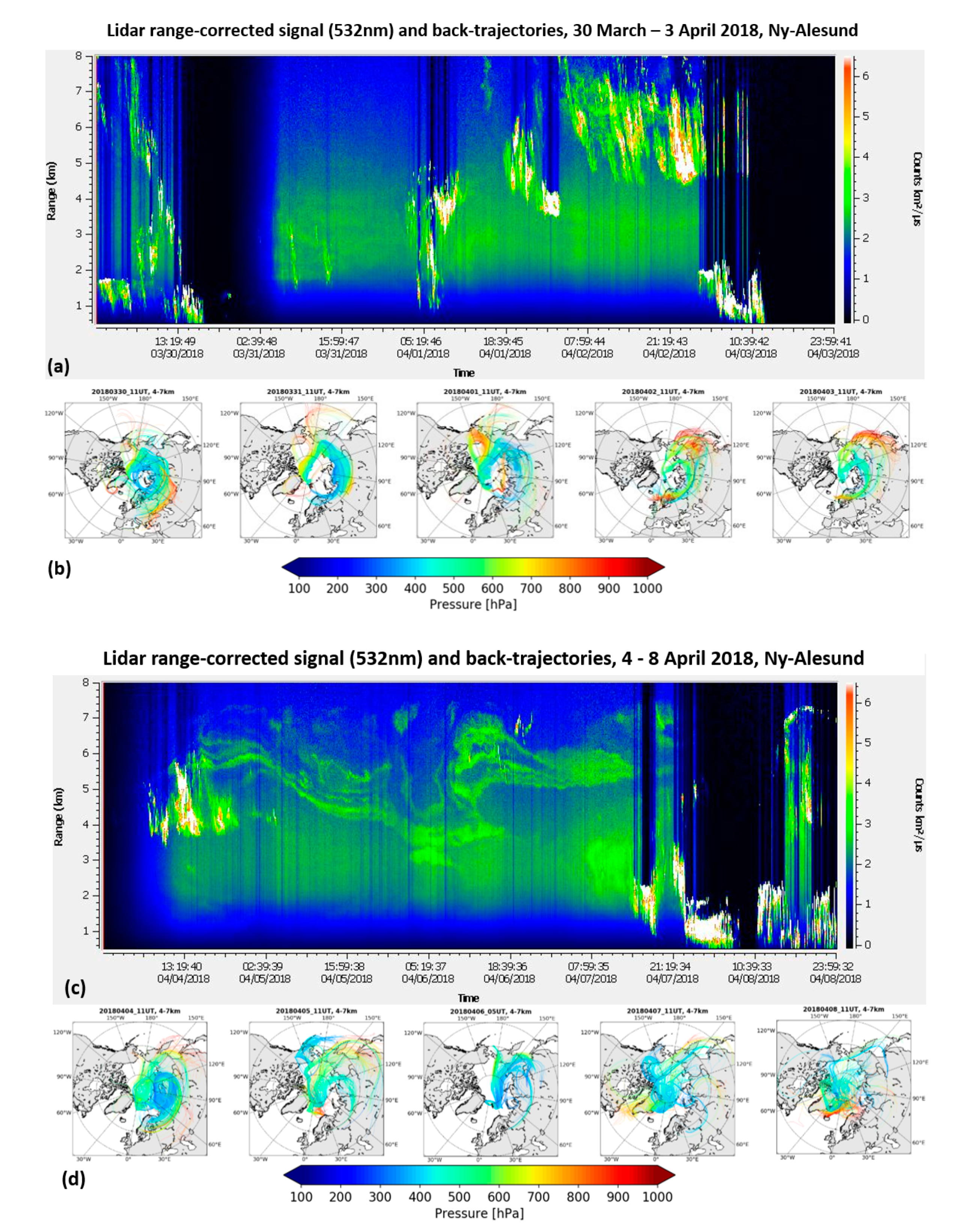
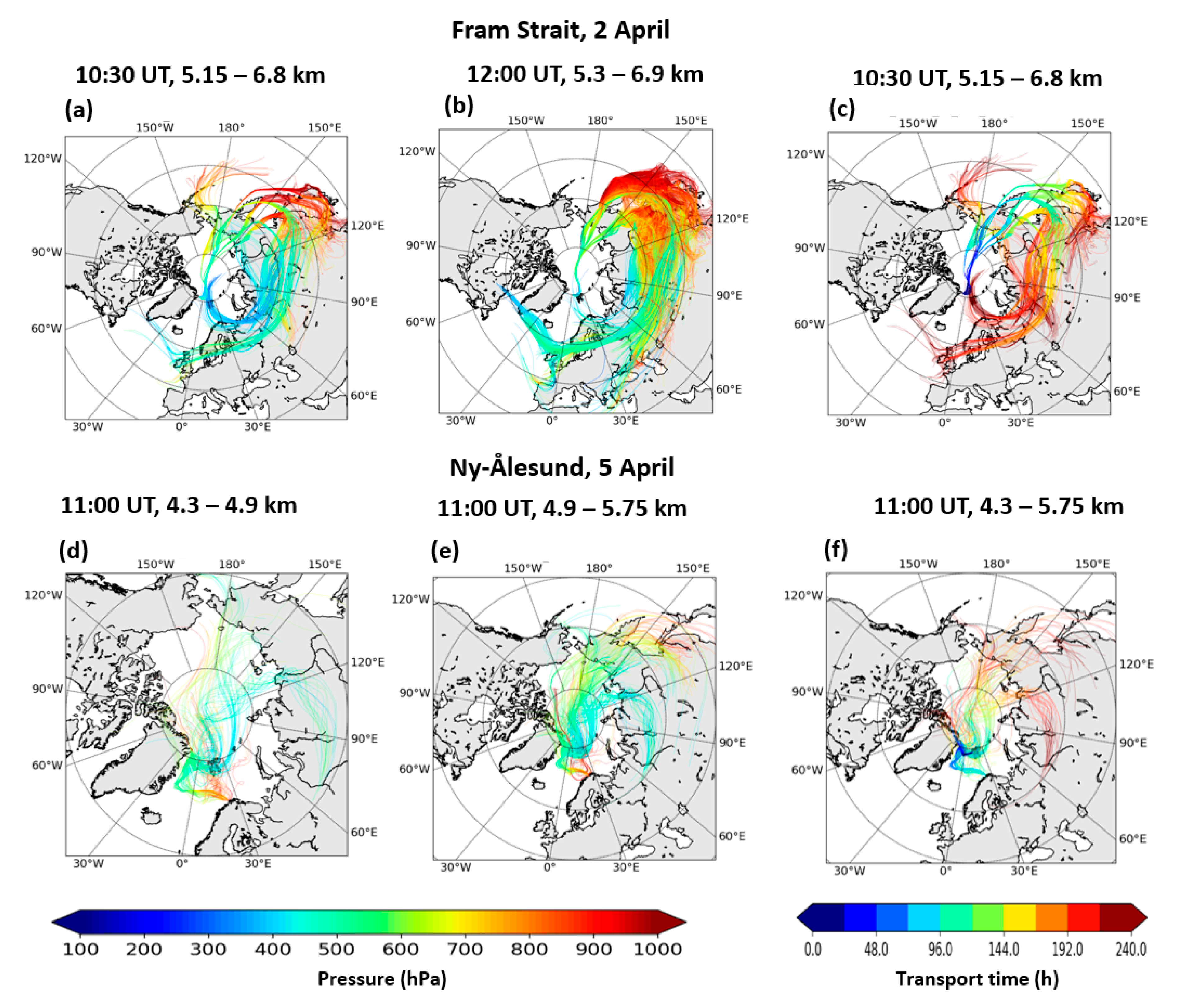
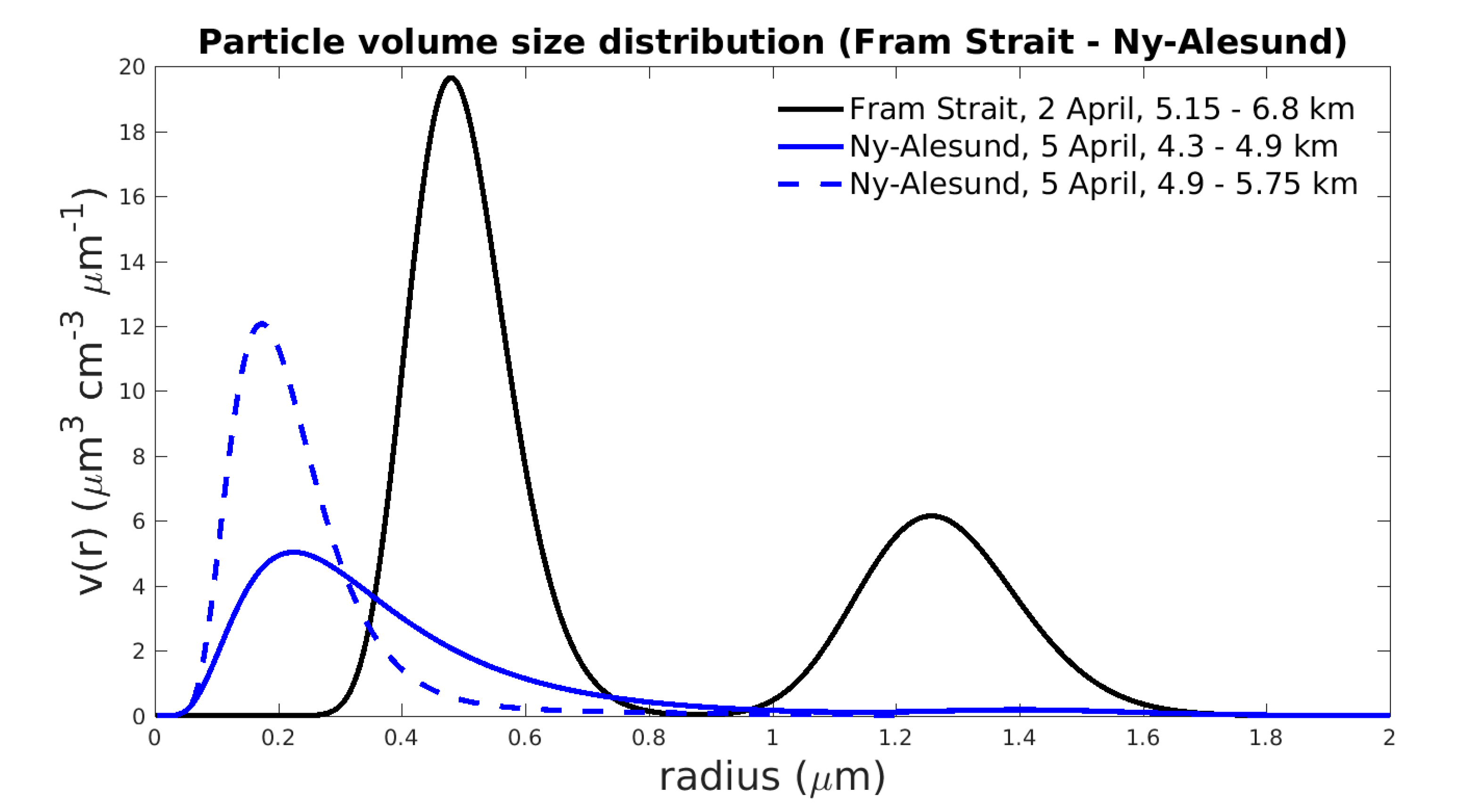
• The aerosol size distribution was clearly modified between the two Arctic locations. The effective radius of the accumulation mode decreased, while the coarse mode was depleted (Figure 9). Industrial pollution and biomass-burning aerosol were funneled to Fram Strait and Ny-Ålesund, Svalbard. In the beginning, aged air masses originating from Asia dominated, while in the course of the episode they mixed with less mature air from northern Europe (Figure 6). Solely, the modified aerosol sources and dry deposition could not account for the elimination of the coarse mode. However, high-level clouds in the interim of the two observations indicate the presence of nucleation scavenging (Figure S1).
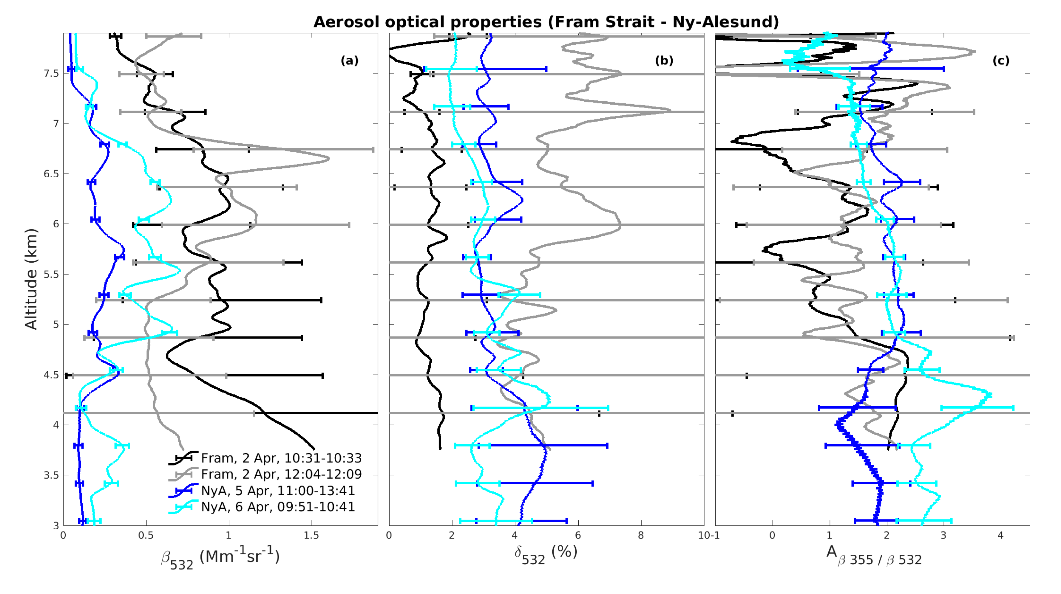
• Along the intra-Arctic transport, particles presented a significantly higher Lidar ratio at visible wavelengths (LR₅₃₂ increased from 15 sr to 64–82 sr). A possible increased absorption can be attributed to black carbon, which could be transported at longer distances as interstitial aerosol since it has low deposition ability [82] and, thus, a longer lifetime. Moreover, black carbon could have been advected through neighboring north European intrusions.
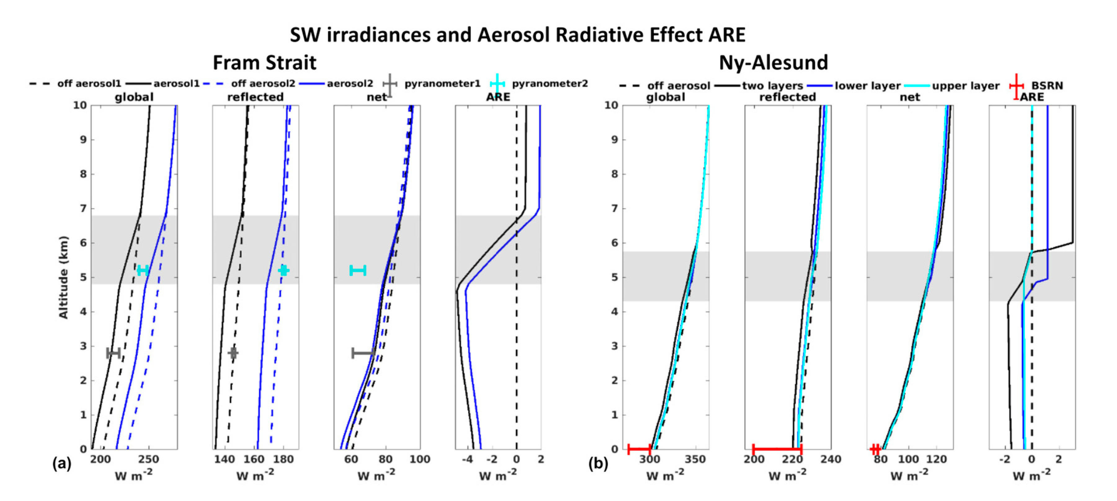
• Despite the coarse mode depletion and increased Lidar ratio, the microphysical similarities of the accumulation mode led to an indistinguishable short-wave radiative footprint in the two episode stages. The accumulation mode drives visible solar irradiance and, thus, dominates the short-wave radiative budget. Thus, the atmospheric column aerosol radiative effect bore similarities over the two locations, amounting to +4.4–4.9 W m⁻² over the ice-covered Fram Strait and +4.5 W m⁻² over the snow-covered Ny-Ålesund. This episode caused top-of-atmosphere warming accompanied by surface cooling, with implications for atmospheric stratification.
• The aerosol radiative effect was more significant compared to the ambient humidity effect on a weekly basis (30% WV mixing ratio perturbation).
• Our study suggests that within this Arctic haze episode, which was dominated by accumulation mode particles, the intra-Arctic aerosol modification (and hence, the precise aerosol microphysics) had little effect on the local radiative budget. However, in the context of retreating Arctic sea ice and declining surface albedo [86], the local aerosol radiative effect may change along individual transport episodes.

References

1. Breider, T.J.; Mickley, L.J.; Jacob, D.J.; Ge, C.; Wang, J.; Payer Sulprizio, M.; Croft, B.; Ridley, D.A.; McConnell, J.R.; Sharma, S. Multidecadal trends in aerosol radiative forcing over the Arctic: Contribution of changes in anthropogenic aerosol to Arctic warming since 1980. J. Geophys. Res. Atmos. 2017, 122, 3573–3594. [Google Scholar] [CrossRef]
2. Bellouin, N.; Quaas, J.; Gryspeerdt, E.; Kinne, S.; Stier, P.; Watson-Parris, D.; Boucher, O.; Carslaw, K.S.; Christensen, M.; Daniau, A.-L. Bounding global aerosol radiative forcing of climate change. Rev. Geophys. 2019, 58, e2019RG000660. [Google Scholar] [CrossRef] [Green Version]
3. Sand, M.; Samset, B.H.; Balkanski, Y.; Bauer, S.; Bellouin, N.; Berntsen, T.K.; Bian, H.; Chin, M.; Diehl, T.; Easter, R. Aerosols at the poles: An AeroCom Phase II multi-model evaluation. Atmos. Chem. Phys. 2017, 17, 12197–12218. [Google Scholar] [CrossRef] [Green Version]
4. Najafi, M.R.; Zwiers, F.W.; Gillett, N.P. Attribution of Arctic temperature change to greenhouse-gas and aerosol influences. Nat. Clim. Chang. 2015, 5, 246–249. [Google Scholar] [CrossRef]
5. Serreze, M.C.; Barry, R.G. Processes and impacts of Arctic amplification: A research synthesis. Glob. Planet. Chang. 2011, 77, 85–96. [Google Scholar] [CrossRef]
6. Wendisch, M.; Brückner, M.; Burrows, J.P.; Crewell, S.; Dethloff, K.; Ebell, K.; Lüpkes, C.; Macke, A.; Notholt, J.; Quaas, J. Understanding causes and effects of rapid warming in the Arctic. Eos 2017, 98. [Google Scholar] [CrossRef]
7. Korhonen, H.; Carslaw, K.S.; Spracklen, D.V.; Ridley, D.A.; Ström, J. A global model study of processes controlling aerosol size distributions in the Arctic spring and summer. J. Geophys. Res. Atmos. 2008, 113. [Google Scholar] [CrossRef] [Green Version]
8. Croft, B.; Martin, R.V.; Leaitch, W.R.; Tunved, P.; Breider, T.J.; D’Andrea, S.D.; Pierce, J.R. Processes controlling the annual cycle of Arctic aerosol number and size distributions. Atmos. Chem. Phys. 2016, 16, 3665–3682. [Google Scholar] [CrossRef] [Green Version]
9. Freud, E.; Krejci, R.; Tunved, P.; Leaitch, R.; Nguyen, Q.T.; Massling, A.; Skov, H.; Barrie, L. Pan-Arctic aerosol number size distributions: Seasonality and transport patterns. Atmos. Chem. Phys. 2017, 17, 8101–8128. [Google Scholar] [CrossRef] [Green Version]
10. Schmeisser, L.; Backman, J.; Ogren, J.A.; Andrews, E.; Asmi, E.; Starkweather, S.; Uttal, T.; Fiebig, M.; Sharma, S.; Eleftheriadis, K. Seasonality of aerosol optical properties in the Arctic. Atmos. Chem. Phys. 2018, 18, 11599–11622. [Google Scholar] [CrossRef] [Green Version]
11. Quinn, P.K.; Shaw, G.; Andrews, E.; Dutton, E.G.; Ruoho-Airola, T.; Gong, S.L. Arctic haze: Current trends and knowledge gaps. Tellus B Chem. Phys. Meteorol. 2007, 59, 99–114. [Google Scholar] [CrossRef] [Green Version]
12. Warneke, C.; Bahreini, R.; Brioude, J.; Brock, C.A.; De Gouw, J.A.; Fahey, D.W.; Froyd, K.D.; Holloway, J.S.; Middlebrook, A.; Miller, L. Biomass burning in Siberia and Kazakhstan as an important source for haze over the Alaskan Arctic in April 2008. Geophys. Res. Lett. 2009, 36. [Google Scholar] [CrossRef] [Green Version]
13. Di Pierro, M.; Jaeglé, L.; Eloranta, E.W.; Sharma, S. Spatial and seasonal distribution of Arctic aerosols observed by CALIOP (2006–2012). Atmos. Chem. Phys. Discuss. 2013, 13, 7075–7095. [Google Scholar] [CrossRef] [Green Version]
14. Ritter, C.; Neuber, R.; Schulz, A.; Markowicz, K.M.; Stachlewska, I.S.; Lisok, J.; Makuch, P.; Pakszys, P.; Markuszewski, P.; Rozwadowska, A. 2014 iAREA campaign on aerosol in Spitsbergen–Part 2: Optical properties from Raman-lidar and in-situ observations at Ny-\AAlesund. Atmos. Environ. 2016, 141, 1–19. [Google Scholar] [CrossRef] [Green Version]
15. Shibata, T.; Shiraishi, K.; Shiobara, M.; Iwasaki, S.; Takano, T. Seasonal Variations in High Arctic Free Tropospheric Aerosols Over Ny-\AAlesund, Svalbard, Observed by Ground-Based Lidar. J. Geophys. Res. Atmos. 2018, 123, 12–353. [Google Scholar] [CrossRef]
16. Klonecki, A.; Hess, P.; Emmons, L.; Smith, L.; Orlando, J. Seasonal changes in the transport of pollutants into the Arctic troposphere-model study: Tropospheric Ozone Production about the Spring Equinox (TOPSE). J. Geophys. Res. 2003, 108, TOP15-1. [Google Scholar] [CrossRef] [Green Version]
17. Stohl, A. Characteristics of atmospheric transport into the Arctic troposphere. J. Geophys. Res. Atmos. 2006, 111, 0148–0227. [Google Scholar] [CrossRef]
18. Di Pierro, M.; Jaeglé, L. Satellite observations of aerosol transport from East Asia to the Arctic: Three case studies. Atmos. Chem. Phys. 2011, 11, 2225. [Google Scholar] [CrossRef] [Green Version]
19. Eleftheriadis, K.; Vratolis, S.; Nyeki, S. Aerosol black carbon in the European Arctic: Measurements at Zeppelin station, Ny-\AAlesund, Svalbard from 1998–2007. Geophys. Res. Lett. 2009, 36. [Google Scholar] [CrossRef] [Green Version]
20. Lisok, J.; Markowicz, K.M.; Ritter, C.; Makuch, P.; Petelski, T.; Chilinski, M.; Kaminski, J.W.; Becagli, S.; Traversi, R.; Udisti, R. 2014 iAREA campaign on aerosol in Spitsbergen–Part 1: Study of physical and chemical properties. Atmos. Environ. 2016, 140, 150–166. [Google Scholar] [CrossRef] [Green Version]
21. Moroni, B.; Arnalds, O.; Dagsson-Waldhauserová, P.; Crocchianti, S.; Vivani, R.; Cappelletti, D. Mineralogical and chemical records of Icelandic dust sources upon Ny-\AAlesund (Svalbard Islands). Front. Earth Sci. 2018, 6, 187. [Google Scholar] [CrossRef]
22. Ferrero, L.; Ritter, C.; Cappelletti, D.; Moroni, B.; Močnik, G.; Mazzola, M.; Lupi, A.; Becagli, S.; Traversi, R.; Cataldi, M. Aerosol optical properties in the Arctic: The role of aerosol chemistry and dust composition in a closure experiment between Lidar and tethered balloon vertical profiles. Sci. Total Environ. 2019, 686, 452–467. [Google Scholar] [CrossRef] [PubMed] [Green Version]
23. Law, K.S.; Stohl, A. Arctic air pollution: Origins and impacts. Science 2007, 315, 1537–1540. [Google Scholar] [CrossRef] [PubMed] [Green Version]
24. Stock, M.; Ritter, C.; Herber, A.; von Hoyningen-Huene, W.; Baibakov, K.; Graeser, J.; Orgis, T.; Treffeisen, R.; Zinoviev, N.; Makshtas, A. Springtime Arctic aerosol: Smoke versus haze, a case study for March 2008. Atmos. Environ. 2012, 52, 48–55. [Google Scholar] [CrossRef] [Green Version]
25. Quennehen, B.; Schwarzenboeck, A.; Matsuki, A.; Burkhart, J.F.; Stohl, A.; Ancellet, G.; Law, K.S. Anthropogenic and forest fire pollution aerosol transported to the Arctic: Observations from the POLARCAT-France spring campaign. Atmos. Chem. Phys. 2012. [Google Scholar] [CrossRef] [Green Version]
26. Monks, S.A.; Arnold, S.R.; Emmons, L.K.; Law, K.S.; Turquety, S.; Duncan, B.N.; Flemming, J.; Huijnen, V.; Tilmes, S.; Langner, J. Multi-model study of chemical and physical controls on transport of anthropogenic and biomass burning pollution to the Arctic. Atmos. Chem. Phys. 2015, 15, 3575–3603. [Google Scholar] [CrossRef] [Green Version]
27. Evangeliou, N.; Balkanski, Y.; Hao, W.; Petkov, A.; Silverstein, R.P.; Corley, R.; Nordgren, B.L.; Urbanski, S.; Eckhardt, S.; Stohl, A. Wildfires in northern Eurasia affect the budget of black carbon in the Arctic-a 12-year retrospective synopsis (2002–2013). Atmos. Chem. Phys. 2016, 16, 7587–7604. [Google Scholar] [CrossRef] [Green Version]
28. Gjelten, H.M.; Nordli, Ø.; Isaksen, K.; Førland, E.J.; Sviashchennikov, P.N.; Wyszynski, P.; Prokhorova, U.V.; Przybylak, R.; Ivanov, B.V.; Urazgildeeva, A.V. Air temperature variations and gradients along the coast and fjords of western Spitsbergen. Polar Res. 2016, 35, 29878. [Google Scholar] [CrossRef]
29. Dahlke, S.; Hughes, N.E.; Wagner, P.M.; Gerland, S.; Wawrzyniak, T.; Ivanov, B.; Maturilli, M. The observed recent surface air temperature development across Svalbard and concurring footprints in local sea ice cover. Int. J. Climatol. 2020. [Google Scholar] [CrossRef]
30. Dahlke, S.; Maturilli, M. Contribution of atmospheric advection to the amplified winter warming in the Arctic North Atlantic region. Adv. Meteorol. 2017, 1687–9309. [Google Scholar] [CrossRef] [Green Version]
31. Woods, C.; Caballero, R.; Svensson, G. Large-scale circulation associated with moisture intrusions into the Arctic during winter. Geophys. Res. Lett. 2013, 40, 4717–4721. [Google Scholar] [CrossRef]
32. Graßl, S.; Ritter, C. Properties of Arctic Aerosol Based on Sun Photometer Long-Term Measurements in Ny-\AAlesund, Svalbard. Remote Sens. 2019, 11, 1362. [Google Scholar] [CrossRef] [Green Version]
33. Binietoglou, I.; D’Amico, G.; Baars, H.; Belegante, L.; Marinou, E. A methodology for cloud masking uncalibrated lidar signals. In Proceedings of the EPJ Web of Conferences; EDP Sciences: Les Ulis, France, 2018; Volume 176, p. 05048. [Google Scholar]
34. Böckmann, C. Hybrid regularization method for the ill-posed inversion of multiwavelength lidar data in the retrieval of aerosol size distributions. Appl. Opt. 2001, 40, 1329–1342. [Google Scholar] [CrossRef] [PubMed]
35. Böckmann, C.; Kirsche, A. Iterative regularization method for lidar remote sensing. Comput. Phys. Commun. 2006, 174, 607–615. [Google Scholar] [CrossRef]
36. Osterloh, L.; Böckmann, C.; Mamouri, R.-E.; Papayannis, A. An adaptive base point algorithm for the retrieval of aerosol microphysical properties. Open Atmos. Sci. J. 2011, 5, 61–73. [Google Scholar] [CrossRef]
37. Samaras, S.; Nicolae, D.; Böckmann, C.; Vasilescu, J.; Binietoglou, I.; Labzovskii, L.; Toanca, F.; Papayannis, A. Using Raman-lidar-based regularized microphysical retrievals and Aerosol Mass Spectrometer measurements for the characterization of biomass burning aerosols. J. Comput. Phys. 2015, 299, 156–174. [Google Scholar] [CrossRef]
38. Stachlewska, I.S.; Neuber, R.; Lampert, A.; Ritter, C.; Wehrle, G. AMALi the Airborne Mobile Aerosol Lidar for Arctic research. Atmos. Chem. Phys. 2010, 10, 2947–2963. [Google Scholar] [CrossRef] [Green Version]
39. Hoffmann, A. Comparative Aerosol Studies Based on Multi-Wavelength Raman LIDAR at Ny-\AAlesund, Spitsbergen. Ph.D. Thesis, University Potsdam, Potsdam, Germany, 2011. [Google Scholar]
40. Iarlori, M.; Madonna, F.; Rizi, V.; Trickl, T.; Amodeo, A. Effective resolution concepts for lidar observations. Atmos. Meas. Tech. Discuss. 2015, 8, 5157–5176. [Google Scholar] [CrossRef] [Green Version]
41. Fernald, F.G. Analysis of atmospheric lidar observations: Some comments. Appl. Opt. 1984, 23, 652–653. [Google Scholar] [CrossRef] [PubMed]
42. Klett, J.D. Stable analytical inversion solution for processing lidar returns. Appl. Opt. 1981, 20, 211–220. [Google Scholar] [CrossRef] [Green Version]
43. Ansmann, A.; Riebesell, M.; Weitkamp, C. Measurement of atmospheric aerosol extinction profiles with a Raman lidar. Opt. Lett. 1990, 15, 746–748. [Google Scholar] [CrossRef] [PubMed]
44. Mei, L.; Vandenbussche, S.; Rozanov, V.; Proestakis, E.; Amiridis, V.; Callewaert, S.; Vountas, M.; Burrows, J.P. On the retrieval of aerosol optical depth over cryosphere using passive remote sensing. Remote Sens. Environ. 2020, 241, 111731. [Google Scholar] [CrossRef]
45. Alexandrov, M.D.; Marshak, A.; Cairns, B.; Lacis, A.A.; Carlson, B.E. Automated cloud screening algorithm for MFRSR data. Geophys. Res. Lett. 2004, 31. [Google Scholar] [CrossRef]
46. Müller, D.; Böckmann, C.; Kolgotin, A.; Schneidenbach, L.; Chemyakin, E.; Rosemann, J.; Znak, P.; Romanov, A. Microphysical particle properties derived from inversion algorithms developed in the framework of EARLINET. Atmos. Meas. Tech. 2016, 9, 5007–5035. [Google Scholar] [CrossRef] [Green Version]
47. Sprenger, M.; Wernli, H. The LAGRANTO Lagrangian analysis tool—Version 2.0. Geosci. Model Dev. 2015, 8, 2569–2586. [Google Scholar] [CrossRef] [Green Version]
48. Wernli, B.H.; Davies, H.C. A Lagrangian-based analysis of extratropical cyclones. I: The method and some applications. Q. J. R. Meteorol. Soc. 1997, 123, 467–489. [Google Scholar] [CrossRef]
49. Ehrlich, A.; Wendisch, M. Reconstruction of high-resolution time series from slow-response broadband terrestrial irradiance measurements by deconvolution. Atmos. Meas. Tech. 2015, 8, 3671–3684. [Google Scholar] [CrossRef] [Green Version]
50. Herber, A. Meteorological Observations during POLAR 5 Campaign PAMARCMIP 2018; Alfred Wegener Institute, Helmholtz Centre for Polar and Marine Research: Bremerhaven, Germany, 2019. [Google Scholar]
51. Burba, G.G.; McDermitt, D.K.; Anderson, D.J.; Furtaw, M.D.; Eckles, R.D. Novel design of an enclosed CO2/H2O gas analyser for eddy covariance flux measurements. Tellus B: Chem. Phys. Meteorol. 2010, 62, 743–748. [Google Scholar] [CrossRef]
52. Maturilli, M.; Herber, A.; König-Langlo, G. Surface radiation climatology for Ny-\AAlesund, Svalbard (78.9 N), basic observations for trend detection. Theor. Appl. Climatol. 2015, 120, 331–339. [Google Scholar] [CrossRef] [Green Version]
53. Maturilli, M. Basic and Other Measurements of Radiation at Station Ny-Ålesund (2018-04); Alfred Wegener Institute—Research Unit Potsdam: Potsdam, Germany, 2018. [Google Scholar]
54. Maturilli, M. High Resolution Radiosonde Measurements from Station Ny-Ålesund (2018-04); Alfred Wegener Institute—Research Unit Potsdam: Potsdam, Germany, 2018. [Google Scholar]
55. Rozanov, V.V.; Rozanov, A.V.; Kokhanovsky, A.A.; Burrows, J.P. Radiative transfer through terrestrial atmosphere and ocean: Software package SCIATRAN. J. Quant. Spectrosc. Radiat. Transf. 2014, 133, 13–71. [Google Scholar] [CrossRef]
56. Rothman, L.S.; Barbe, A.; Benner, D.C.; Brown, L.R.; Camy-Peyret, C.; Carleer, M.R.; Chance, K.; Clerbaux, C.; Dana, V.; Devi, V.M. The HITRAN molecular spectroscopic database: Edition of 2000 including updates through 2001. J. Quant. Spectrosc. Radiat. Transf. 2003, 82, 5–44. [Google Scholar] [CrossRef]
57. Sinnhuber, B.-M.; Sheode, N.; Sinnhuber, M.; Chipperfield, M.P.; Feng, W. The contribution of anthropogenic bromine emissions to past stratospheric ozone trends: A modelling study. Atmos. Chem. Phys. 2009, 9, 2863–2871. [Google Scholar] [CrossRef] [Green Version]
58. Yamanouchi, T.; Treffeisen, R.; Herber, A.; Shiobara, M.; Yamagata, S.; Hara, K.; Sato, K.; Yabuki, M.; Tomikawa, Y.; Rinke, A. Arctic study of tropospheric aerosol and radiation (ASTAR) 2000: Arctic haze case study. Tellus B: Chem. Phys. Meteorol. 2005, 57, 141–152. [Google Scholar] [CrossRef]
59. Lazaridis, M.; Hov, Ø.; Eleftheriadis, K. Heterogeneous nucleation on rough surfaces: Implications to atmospheric aerosols. Atmos. Res. 2000, 55, 103–113. [Google Scholar] [CrossRef]
60. Hoffmann, A.; Osterloh, L.; Stone, R.; Lampert, A.; Ritter, C.; Stock, M.; Tunved, P.; Hennig, T.; Böckmann, C.; Li, S.-M. Remote sensing and in-situ measurements of tropospheric aerosol, a PAMARCMiP case study. Atmos. Environ. 2012, 52, 56–66. [Google Scholar] [CrossRef] [Green Version]
61. Ritter, C.; Angeles Burgos, M.; Böckmann, C.; Mateos, D.; Lisok, J.; Markowicz, K.M.; Moroni, B.; Cappelletti, D.; Udisti, R.; Maturilli, M. Microphysical properties and radiative impact of an intense biomass burning aerosol event measured over Ny-\AAlesund, Spitsbergen in July 2015. Tellus B Chem. Phys. Meteorol. 2018, 70, 1–23. [Google Scholar] [CrossRef]
62. Schacht, J.; Heinold, B.; Quaas, J.; Backman, J.; Cherian, R.; Ehrlich, A.; Herber, A.; Huang, W.T.; Kondo, Y.; Massling, A. The importance of the representation of air pollution emissions for the modeled distribution and radiative effects of black carbon in the Arctic. Atmos. Chem. Phys. 2019, 19, 11159–11183. [Google Scholar] [CrossRef] [Green Version]
63. Schwarz, J.P.; Weinzierl, B.; Samset, B.H.; Dollner, M.; Heimerl, K.; Markovic, M.Z.; Perring, A.E.; Ziemba, L. Aircraft measurements of black carbon vertical profiles show upper tropospheric variability and stability. Geophys. Res. Lett. 2017, 44, 1132–1140. [Google Scholar] [CrossRef]
64. Schwarz, J.P.; Samset, B.H.; Perring, A.E.; Spackman, J.R.; Gao, R.S.; Stier, P.; Schulz, M.; Moore, F.L.; Ray, E.A.; Fahey, D.W. Global-scale seasonally resolved black carbon vertical profiles over the Pacific. Geophys. Res. Lett. 2013, 40, 5542–5547. [Google Scholar] [CrossRef] [Green Version]
65. Mizuta, R. Intensification of extratropical cyclones associated with the polar jet change in the CMIP5 global warming projections. Geophys. Res. Lett. 2012, 39. [Google Scholar] [CrossRef] [Green Version]
66. Lambert, S.J.; Fyfe, J.C. Changes in winter cyclone frequencies and strengths simulated in enhanced greenhouse warming experiments: Results from the models participating in the IPCC diagnostic exercise. Clim. Dyn. 2006, 26, 713–728. [Google Scholar] [CrossRef]
67. Barriopedro, D.; García-Herrera, R.; Lupo, A.R.; Hernández, E. A Climatology of Northern Hemisphere Blocking. J. Clim. 2006, 19, 1042–1063. [Google Scholar] [CrossRef] [Green Version]
68. Garrett, T.; Zhao, C.; Novelli, P. Assessing the relative contributions of transport efficiency and scavenging to seasonal variability in Arctic aerosol. Tellus B Chem. Phys. Meteorol. 2010, 62, 190–196. [Google Scholar] [CrossRef]
69. Seinfeld, J.H.; Pandis, S.N. Atmospheric Chemistry and Physics: From Air Pollution to Climate Change; John Wiley & Sons: Hoboken, NJ, USA, 2016. [Google Scholar]
70. Fletcher, N.H.J. Size effect in heterogeneous nucleation. J. Chem. Phys. 1958, 29, 572–576. [Google Scholar] [CrossRef]
71. Nicolae, D.; Nemuc, A.; Müller, D.; Talianu, C.; Vasilescu, J.; Belegante, L.; Kolgotin, A. Characterization of fresh and aged biomass burning events using multiwavelength Raman lidar and mass spectrometry. J. Geophys. Res. Atmos. 2013, 118, 2956–2965. [Google Scholar] [CrossRef]
72. Hoffmann, A.; Ritter, C.; Stock, M.; Shiobara, M.; Lampert, A.; Maturilli, M.; Orgis, T.; Neuber, R.; Herber, A. Ground-based lidar measurements from Ny-\AAlesund during ASTAR 2007: A statistical overview. Atmos. Chem. Phys. Discuss 2009, 9, 15453–15510. [Google Scholar] [CrossRef]
73. Tunved, P.; Ström, J.; Krejci, R. Arctic aerosol life cycle: Linking aerosol size distributions observed between 2000 and 2010 with air mass transport and precipitation at Zeppelin station, Ny-\AA lesund, Svalbard. Atmos. Chem. Phys. 2013, 13, 3643–3660. [Google Scholar] [CrossRef] [Green Version]
74. Mei, L.; Rozanov, V.; Ritter, C.; Heinold, B.; Jiao, Z.; Vountas, M.; Burrows, J.P. Retrieval of aerosol optical thickness in the Arctic snow-covered regions using passive remote sensing: Impact of aerosol typing and surface reflection model. IEEE Trans. Geosci. Remote Sens. 2020, 58, 5117–5131. [Google Scholar] [CrossRef]
75. Janicka, L.; Stachlewska, I.S.; Veselovskii, I.; Baars, H. Temporal variations in optical and microphysical properties of mineral dust and biomass burning aerosol derived from daytime Raman lidar observations over Warsaw, Poland. Atmos. Environ. 2017, 169, 162–174. [Google Scholar] [CrossRef]
76. Ortiz-Amezcua, P.; Guerrero-Rascado, J.L.; Granados-Muñoz, M.J.; Benavent-Oltra, J.A.; Böckmann, C.; Samaras, S.; Stachlewska, I.S.; Janicka, L.; Baars, H.; Bohlmann, S. Microphysical characterization of long-range transported biomass burning particles from North America at three EARLINET stations. Atmos. Chem. Phys. 2019, 17, 5931–5946. [Google Scholar] [CrossRef] [Green Version]
77. Giannakaki, E.; Van Zyl, P.G.; Müller, D.; Balis, D.; Komppula, M. Optical and microphysical characterization of aerosol layers over South Africa by means of multi-wavelength depolarization and Raman lidar measurements. Atmos. Chem. Phys. 2016, 16, 8109–8123. [Google Scholar] [CrossRef] [Green Version]
78. Haarig, M.; Ansmann, A.; Baars, H.; Jimenez, C.; Veselovskii, I.; Engelmann, R.; Althausen, D. Depolarization and lidar ratios at 355, 532, and 1064 nm and microphysical properties of aged tropospheric and stratospheric Canadian wildfire smoke. Atmos. Chem. Phys. 2018, 18, 11847–11861. [Google Scholar] [CrossRef] [Green Version]
79. Janicka, L.; Stachlewska, I.S. Properties of biomass burning aerosol mixtures derived at fine temporal and spatial scales from Raman lidar measurements: Part I optical properties. Atmos. Chem. Phys. Discuss 2019, 1–46. [Google Scholar] [CrossRef] [Green Version]
80. Groß, S.; Esselborn, M.; Weinzierl, B.; Wirth, M.; Fix, A.; Petzold, A. Aerosol classification by airborne high spectral resolution lidar observations. Atmos. Chem. Phys. 2013, 13, 2487. [Google Scholar] [CrossRef] [Green Version]
81. Donth, T.; Jäkel, E.; Ehrlich, A.; Heinold, B.; Schacht, J.; Herber, A.; Zanatta, M.; Wendisch, M. Combining atmospheric and snow layer radiative transfer models to assess the solar radiative effects of black carbon in the Arctic. Atmos. Chem. Phys. Discuss. 2020, 1–26. [Google Scholar] [CrossRef] [Green Version]
82. Macdonald, K.M.; Sharma, S.; Toom, D.; Chivulescu, A.; Hanna, S.; Bertram, A.K.; Platt, A.; Elsasser, M.; Huang, L.; Tarasick, D. Observations of atmospheric chemical deposition to high Arctic snow. Atmos. Chem. Phys. 2017, 17, 5775–5788. [Google Scholar] [CrossRef] [Green Version]
83. Papagiannopoulos, N.; Alados Arboledas, L.; Guerrero-Rascado, J.L. An automatic observation-based aerosol typing method for EARLINET. Atmos. Chem. Phys. 2018, 18, 15879–15901. [Google Scholar] [CrossRef] [Green Version]
84. Giannakaki, E.; Kokkalis, P.; Marinou, E.; Bartsotas, N.S.; Amiridis, V.; Ansmann, A.; Komppula, M. The potential of elastic and polarization lidars to retrieve extinction profiles. Atmos. Meas. Tech. 2020, 13, 893–905. [Google Scholar] [CrossRef] [Green Version]
85. Zielinski, T.; Bolzacchini, E.; Cataldi, M.; Ferrero, L.; Graßl, S.; Hansen, G.; Mateos, D.; Mazzola, M.; Neuber, R.; Pakszys, P.; et al. Study of Chemical and Optical Properties of Biomass Burning Aerosols during Long-Range Transport Events toward the Arctic in Summer 2017. Atmosphere 2020, 11, 84. [Google Scholar] [CrossRef] [Green Version]
86. Döscher, R.; Vihma, T.; Maksimovich, E. Recent advances in understanding the Arctic climate system state and change from a sea ice perspective: A review. Atmos. Chem. Phys. 2014, 14, 13571–13600. [Google Scholar] [CrossRef] [Green Version]
Figure 1. Flight track of Polar 5 during the outbound leg of the research flight over Fram on 2 April. The flight altitude is color-indicated. Polar 5 took off from Villum Research Station, Greenland, and performed a transect flight over Fram Strait. AMALi (10:31–10:33 and 12:04–12:09) and sun-photometer (10:52–10:57) observations were exploited synergistically. The aerosol properties evaluation periods are indicated with grey shading.
Remotesensing 12 02112 g001
Figure 2. Persistent high tropospheric aerosol layers observed over Fram Strait and Ny-Alesund, Svalbard, by AMALi and MPL systems, respectively. The Lidar range-corrected signal over Fram Strait (a) and Ny-Ålesund (b) is shown. The evaluation periods of aerosol optical and microphysical properties are indicated with solid rectangles. Dashed rectangles denote periods where only the optical properties were evaluated, due to the lack of air-borne photometer and Raman Lidar observations at Fram Strait and Ny-Ålesund, respectively. Thick clouds over Ny-Ålesund did not allow for Raman Lidar observations in the interim days.
Remotesensing 12 02112 g002
Figure 3. Evolution of aerosol optical depth (AOD) over Fram Strait obtained from the air-borne sun-photometer. A persistent aerosol layer was observed at 5.15 km. Selected measurement points (1–5) were used for estimating the aerosol extinction coefficient of the layer. These observations were combined with Raman Lidar measurements. For details, see Section 2.2. Note the changing flight altitude during the measurements.
Remotesensing 12 02112 g003
Figure 4. Evolution of the long-range transport episode over Ny-Ålesund. The MPL range-corrected signal is displayed (a and c) and LAGRANTO backward trajectories (b and d) with arrival height at 4–7 km. Increased aerosol burden air masses were funneled from northeast Asia and north Europe (2–5 April). Persistent elevated aerosol layers (approximately at 4–7 km) were observed on 5–7 April.
Remotesensing 12 02112 g004
Figure 5. Evolution of AOD over Ny-Ålesund derived from sun-photometer, after cloud screening. For comparison, the AOD over Fram Strait as derived from the air-borne sun-photometer is given (average ± one standard deviation). Overall, the AOD over Ny-Ålesund was significantly lower than Fram Strait, reflecting the effect of removal processes and modified aerosol source efficiency.
Remotesensing 12 02112 g005
Figure 6. Backward trajectories ending at the aerosol layer altitude sectors over Fram Strait (ac) and Ny-Ålesund (df). Atmospheric pressure (a, b, d, and e) and transport time (c and f) of the trajectories are color indicated. The transport time corresponds to air masses arriving at the Greenland side of Fram Strait as well as to both aerosol layer altitude sectors at Ny-Alesund (c and f). Aged Asian air masses affected Fram Strait. Ny-Ålesund was influenced by Asian and fresher air masses from north Europe. The latter air masses mixed over Fram Strait two to three days earlier (f).
Remotesensing 12 02112 g006
Figure 7. Aerosol optical properties over Fram Strait (Fram) and Ny-Ålesund (NyA) derived from the air-borne AMALi and ground-based KARL systems, respectively. The aerosol backscatter coefficient β, aerosol depolarization ratio δ, and backscatter-related Angström exponent Aβ are presented. Error bars represent retrieval uncertainties (for details, see Section 2.1). Air-borne profiles exhibit higher uncertainties due to flight altitude changes that constrained the temporal averaging. The aerosol load was higher over Fram Strait (higher β, a). For both locations, particles were nearly spherical (low δ, b). A shift towards smaller particles was observed over Ny-Ålesund (higher Aβ, c).
Remotesensing 12 02112 g007
Figure 8. Aerosol extinction coefficient α (ab) over Fram Strait (2 April) derived from the air-borne photometer (black dots) and from its synergy with Raman Lidar (black squares) as well as over Ny-Ålesund (5 April) from Raman Lidar (blue dots). The corresponding extinction-related Angström exponent is also demonstrated (c). Horizontal error bars indicate the uncertainties according to error propagation. Vertical error bars indicate the altitude sectors where the α was derived (for details, see Section 2.2). The α over Fram Strait was calculated by Equation (2). At the visible spectrum, α was similar over both locations (a). However, at near-infrared, α diminished significantly over Ny-Ålesund (b).
Remotesensing 12 02112 g008
Figure 9. Particle volume size distributions over Fram Strait and Ny-Ålesund retrieved by regularization techniques (for details, see Section 2.3). A clear diminishing of the coarse aerosol mode was revealed for Ny-Ålesund.
Remotesensing 12 02112 g009
Figure 10. Altitude-dependent SW simulated irradiances and aerosol radiative effect (ARE) for AMALi (1) and sun-photometer (2) evaluation periods over Fram Strait (a) and over Ny-Ålesund (b). Observed irradiances are given for comparison (average ± one standard deviation). The aerosol layer altitude is indicated with grey shading. Over both locations, TOA warming was accompanied by surface cooling. Note the different scales.
Remotesensing 12 02112 g010