A New and Simplified Approach for Estimating the Daily River Discharge of the Tibetan Plateau Using Satellite Precipitation: An Initial Study on the Upper Brahmaputra River

Abstract

Collecting in situ observations from remote, high mountain rivers presents major challenges, yet real-time, high temporal resolution (e.g., daily) discharge data are critical for flood hazard mitigation and river management. In this study, we propose a method for estimating daily river discharge (RD) based on free, operational remote sensing precipitation data (Tropical Rainfall Measuring Mission (TRMM), since 2001). In this method, an exponential filter was implemented to produce a new precipitation time series from daily basin-averaged precipitation data to model the time lag of precipitation in supplying RD, and a linear-regression relationship was constructed between the filtered precipitation time series and observed discharge records. Because of different time lags in the wet season (rainfall-dominant) and dry season (snowfall-dominant), the precipitation data were processed in a segmented way (from June to October and from November to May). The method was evaluated at two hydrological gauging stations in the Upper Brahmaputra (UB) river basin, where Nash–Sutcliffe Efficiency (NSE) coefficients for Nuxia (>0.85) and Yangcun (>0.80) indicate good performance. By using the degree-day method to estimate the snowmelt and acquire the time series of new active precipitation (rainfall plus snowmelt) in the target basins, the discharge estimations were improved (NSE > 0.9 for Nuxia) compared to the original data. This makes the method applicable for most rivers on the Tibetan Plateau, which are fed mainly by precipitation (including snowfall) and are subject to limited human interference. The method also performs well for reanalysis precipitation data (Chinese Meteorological Forcing Dataset (CMFD), 1980–2000). The real-time or historical discharges can be derived from satellite precipitation data (or reanalysis data for earlier historical years) by using our method.

1. Introduction

River discharge (RD) data are indispensable for water resources management and flood prediction, and are also important for climate change studies and hydrological modeling [1,2,3]. RD data are traditionally obtained by monitoring river hydrological variables (depth, width, and velocity) at river gauging stations. However, in some areas, particularly those in mountainous regions such as the Tibetan Plateau (TP), collecting the real-time measurements needed for flood forecasting and hazard mitigation presents significant challenges [4].

The TP is the source of more than 10 large rivers, including the Yangtze River, Yellow River, and Ganges [5], which provides water for billions of people and numerous ecosystems. The rivers on the TP are typical mountain rivers, in which the streamflow is mainly affected by climate change, and there is little or negligible direct human interference [6]. Because of rapid warming on the TP, the risk of extreme flood events is increasing [7], leading to a greater demand for timely and high temporal resolution discharge data for flood prediction and mitigation (e.g., barrier lakes). However, data from hydrological gauging stations are sometimes discontinuous, because the remote and harsh mountain environment entails costly maintenance.

Hydrological modeling has been employed for estimating and predicting RD [8,9,10,11], but high accuracy demands a precise description of the most significant hydrological processes within the catchment, and therefore requires abundant data describing the topography, soil, hydrology, land cover, and forcing data [12,13]. The TP is an environment with many interacting spheres [14], such that its hydrology is complex and difficult to model, yet meteorological and hydrological observations are sparse [15]. Without adequate observations for the assessment and validation of operational models, uncertainties in the model output can be significant.

The development of satellite and remote sensing technologies has made it feasible to continue the runoff records for rivers with conventional measurements [16]. In recent decades, several methods for remote discharge estimation have been developed based on various satellite data sources, such as optical imagery, radar imagery, as well as data from altimetry and microwave scanning radiometry [17,18,19,20,21]. Nevertheless, it is still difficult to acquire remote sensing discharge records at temporal sampling rates matching those of gauging stations [22].

Discharge estimates based on remote sensing can be divided into single-variable and multiple-variable groups. Multiple-variable methods consider hydraulic elements related to runoff that can be retrieved from satellite data, with different variables using indifferent formulas [23,24]. The temporal sampling rate of multiple-variable estimates is likely to be low, as multiple variables cannot usually be observed at the same time [1,25,26]. Estimates based on single-variable methods are mainly achieved by constructing statistical relationships between remote-sensing-derived hydrological variables (stage or width) and observed discharges [27,28]. Optical images used for estimating river width have varying temporal resolution, with high temporal resolution sources (e.g., Moderate Resolution Imaging Spectroradiometer, MODIS) normally having low spatial resolution [29], which is not suitable for mountainous regions, where rivers are usually small (width < 400 m) [18]. Cloudy weather in the rainy season also hinders the use of optical images [30]. Although remote sensing methods based on multi-location stages have been developed to derive daily discharge, they are not suitable for small rivers [31,32].

With the development of satellite technology for monitoring precipitation, it is possible to estimate river discharge based on remote sensing precipitation. The main drawback for discharge estimating in mountainous rivers is that the width and stage cannot both be measured accurately and frequently with remote sensing. However, operational remote sensing precipitation data have high temporal resolution (daily or better) and can satisfy the temporal resolution requirements.

The main objective of this study is to develop a method for daily discharge estimation based on discharge observations and operational remote sensing precipitation. The method is demonstrated at two locations on the Upper Brahmaputra (UB, Yarlung Zangbo) river basin, Tibetan Plateau. Considering that the remote sensing precipitation data have been available since 1998, the method is also used to process a reanalysis precipitation dataset to estimate daily discharge before 1998. The rest of the paper is organized as follows. Section 2 introduces the study regions. Section 3 describes the data that were used and the method that was developed in the study. Section 4 presents the discharge estimates and performance of the method. Section 5 discusses the impact factors for the method and concludes the utilities of the method.

2. Study Regions

The UB river basin is located in the south of the Tibet Plateau (TP) (Figure 1) and covers an area of around 241,000 km². The river basin is in the upstream region of the Brahmaputra River, a trans-boundary river that flows through China, India, and Bangladesh. With an average elevation of 4000 m above sea level, the Upper Brahmaputra river is the world’s highest river. The TP is one of the most sensitive regions to climate change [33], and understanding changes in river discharge on the TP is important for climate change studies; however, the region’s remoteness, high altitude, and harsh weather conditions make field observations difficult and expensive.

The width for the UB river ranges from <100 m in winter to nearly 500 m in summer. The rainy season is June to September (the Indian monsoon season), which accounts for 60–80% of the annual precipitation [34]. Two gauging stations (Nuxia and Yangcun) were used to validate our approach in the study area (Figure 1). Both catchments above the two stations are fed mainly by precipitation (rain and snow), as glaciers occupy only a small proportion (

Table 1. The area and relative proportion of glaciers in the basins upstream of Nuxia and Yangcun hydrological stations.

Station Name	Basin Area above the Station (km2)	Glacier Area in the Basin above the Station (km2)	Areal Proportion of Glaciers (%)
Yangcun	156,561	1793	1.14
Nuxia	195,766	3183	1.63

). In a preceding study, which simulated the discharge with a variable infiltration capacity (VIC) model [35], the contribution of glacier melt to RD was about 10% in the basin.

3. Data and Method

3.1. Datasets

Two types of operational precipitation data were used to test our method: satellite precipitation data and reanalysis precipitation data. The satellite precipitation data were acquired from the Tropical Rainfall Measuring Mission (TRMM) Multi-Satellite Precipitation Analysis (TMPA) and the reanalysis precipitation data were from the Chinese Meteorological Forcing Dataset (CMFD). These are among the most popular satellite precipitation products and they have been applied and evaluated in other basins [36,37,38,39].

The TRMM satellite is a rain-monitoring meteorological satellite that was jointly launched by the American National Aeronautics and Space Administration (NASA) and the Japanese National Space Development Agency (NASDA) in 1997 [40]. The TRMM_3B42_Daily dataset, a quasi-global (50°S–50°N, 180°E–180°W), three-level precipitation product of TRMM satellites, was used in this study. It is a fusion of data from TMI (microwave imager), SSMI (special microwave imaging sensor), AMSR (enhanced microwave scanning radiometer), AMSU (advanced microwave), and thermal infrared sensors. This dataset contained 0.25° × 0.25° daily precipitation accumulation data generated from the research-quality 3-hourly TMPA precipitation data [41]. A total of 6328 files (from 1 January 2001 to 29 April 2018) were used in this study.

The China Meteorological Forcing Dataset (CMFD) is a near-surface meteorological and environmental reanalysis dataset developed by the Institute of Tibetan Plateau Research at the Chinese Academy of Science [42]. The dataset is based on the Princeton reanalysis data, GEWEX-SRB, GLDAS, and TRMM precipitation data, combined with meteorological data from the China Meteorological Administration. Its resolution is 0.1°. In this study, the daily precipitation product for the period 1979–2018 is used, including 15,460 files (from 1 January 1979 to 29 April 2018). The daily precipitation data were computed from the 3 h precipitation data.

In the process of snowmelt estimation, the daily temperature data used for differentiating rain and snow as well as the calculation of snowmelt were also from CMFD. Daily temperature (from 1 January 1979 to 29 April 2018) was used to split rainfall and snowfall, as well as to calculate daily snowmelt based on a degree-day model. The extracted rainfall and snowfall data between 1 January 2001 and 31 December 2010 were used to compute the multi-year monthly mean precipitation of rain and snow.

Observed discharge data included daily data and monthly data. Daily data were available for Nuxia station (2001 to 2018) and Yangcun station (2003 to 2015). As daily data were not available before 2000, we used monthly data to evaluate historically simulated discharge. All the discharge data were processed into the normalized form.

3.2. Methods

3.2.1. Basin-Averaged Precipitation

Our method attempted to estimate daily discharge by constructing a statistical relationship between operational precipitation data and observed discharge. The basin-averaged precipitation over the study catchment was computed and used as the input of the method. The average precipitation data for the two catchments (Figure 1) were obtained by clipping and statistical analysis. To compute the average precipitation over the basin, we resampled the original data into uniform grids (5 × 5 km).

3.2.2. Exponential Filter

The exponential filter was used to model the time lag of the precipitation supply for the RD. There was an obvious delay in the peak discharge relative to the basin-averaged precipitation peak (Figure 2), resulting in poor correlation between the original average precipitation and observed discharge. The discharge often has a time lag relative to the supplements of both rainfall and snowfall because of the storage in a river system, while the time length is different. Physically, the discharge is correlated to the total precipitation over several days before the discharge observation time. Moreover, precipitation closer to the observation time has a greater contribution to the measured discharge. Therefore, an exponential filter [43,44] was applied to process the average precipitation data time series, which was continually calculated as a weighted average of recent precipitation data by giving less weight to older data. A new time series of precipitation data were acquired through the exponential filter. This filter uses a single tuning parameter named the characteristic time T. The correlation coefficient between filtered precipitation and observed discharge changes when T changes. When the correlation coefficient reaches the maximum, the value of T is defined as T_peak. The new time series of precipitation was calculated by using the exponential filter and setting T as T_peak.

The exponential filter uses a recursive formula [43]:

$$P_{t_{n+1}}^{\ast }=P_{t_n}^{\ast }+K_{t_{n+1}}\left(P_{t_{n+1}}-P_{t_n}^{\ast }\right)$$

(1)

$$K_{t_{n+1}}=\frac{K_{t_n}}{K_{t_n}+e^{-\left(\frac{t_{n+1}-t_n}{T}\right)}}$$

(2)

where $P_{t_{n+1}}$ is the average precipitation at time $t_{n+1}$ and $P_{t_n}^{\ast }$ is the respective filtered value at the previous time $t_n$. T is the characteristic time and K ranges between 0 and 1. To initialize the filter, $K_{t_1}$ and $P_{t_1}^{\ast }$ were set to 1 and $P_{t_1}$ (the precipitation for the first day in the records), respectively.

3.2.3. Linear Least-Squares Regression

After the value of T_peak was determined and the corresponding filtered basin-averaged precipitation was obtained, a linear least-squares regression model was constructed with the filtered average precipitation as the independent variable and observed discharge as the dependent variable. Discharge for the times without observations was then estimated using the linear regression model. The filtering and linear regression (FLR) method is summarized in a flow chart (Figure 3).

3.2.4. Segmented Processing of Precipitation Data

Due to the high elevation of the UB river basin above sea level, both rainfall and snowfall are supplies for the discharge. In the wet season, rainfall is the dominant supply, while snowmelt is more important in the dry season. To distinguish the wet season and dry season, the multi-year monthly mean basin-averaged rainfall and snowfall were calculated by applying a relationship between air temperature and precipitation type constructed by Ding et al. [45]. The study of Ding et al. presented the function relationship of proportions of precipitation types with surface elevation and temperature. The multi-year mean monthly precipitation of rain and snow is presented in Figure 4. It shows that the precipitation over the UB river basin is mainly rainfall from June to August. In September and October, although there is less rainfall than snowfall, it is still the dominant supply for the RD, considering the time lag of the confluence. Additionally, the snowfall over the two months melts quickly due to the warm temperature. Therefore, the wet season includes summer and autumn, while the dry season includes winter and spring for the UB river basin. Therefore, basin-averaged precipitation from June to October (wet season) and precipitation data from November to the next May (dry season) are processed separately (Figure 3).

Considering the different dominant types of precipitation in wet seasons and dry seasons, the segmented method was used to deal with the basin-averaged precipitation instead of the year-round method. Discharge often has different time lags relative to the supplements of both rainfall and snowfall, so the wet season (rainfall dominant, warm) and dry season (snow dominant, cold) are separated for estimation (Figure 3). In the segmented method, all the processes are doubled and T_peak has two values. The two values of T_peak are acquired by recognizing the max correlation coefficients in two periods (the wet season and dry season, respectively).

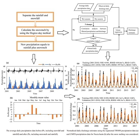
3.2.5. Calculation of Snowmelt

Differing from rainfall, the contribution of snowfall to discharge is more complex. It includes the accumulation and melting of snow. To explicitly study the impact of snow melting on discharge estimation by using the FLR, we used the degree-day method (DDM) [46] to simply estimate the snow melt. After using the DDM to calculate the snowmelt, the summation of daily snowmelt and rainfall produced a new basin-averaged total liquid water (hereafter the active precipitation, Pa) received by the target basin. The time series of active precipitation at each grid cell (5 × 5 km) in this study can be computed through the following procedures:

(1)

Separate the rainfall (Pr) and snowfall (Ps) from the daily precipitation data by using the method provided by Ding et al. [45];

(2)

Calculate the potential snowmelt capacity (SMc) by using the DDM;

(3)

If SMc > Ps, the actual snowmelt (SMa) is equal to the snowfall (that is SMa = Ps); otherwise SMa = SMc, and the value of Ps minus SMc is added to the Ps of the next day;

(4)

The daily active precipitation Pa is equal to the summation of Pr and SMa (Pa = Pr + SMa).

After calculating the Pa for all the grid cells in the target basin, then the basin-averaged Pa can be obtained. The new basin-averaged active precipitation Pa is then processed by using the FLR method and the estimation of RD is compared with the result from the original precipitation data to assess the impacts of snowfall and snow melting on the discharge estimation.

The equations to compute the potential snowmelt capacity are listed as follows:

$$SMc=DDF\ast PDD$$

(3)

$$PDD={\displaystyle \sum }_{t=1}^n{H}_t·T_t$$

(4)

where DDF (mm/d/°C) is the degree-day factor and PDD (°C) is the positive degrees in a day. DDF is an empirical parameter. The DDF used in the study is obtained by the method provide by Liu and Zhang [47], who developed an algorithm to spatially estimate the positive DDFs based on available observed DDFs. The spatial distribution of DDFs in the Yarlung Zangbo River Basin were presented in the paper. Here, $T_t$ is the daily temperature and $H_t$ is a logical variable ($H_t=1.0 \mathrm{when} T_t\ge 0; H_t=0.0 \mathrm{when} T_t<0$).

3.2.6. Performance Evaluation

The accuracy of the discharge estimates was determined by using different performance measures, such as the Nash–Sutcliffe efficiency coefficient (NSE) [48], the root mean square error (RMSE), and the BIAS, which are defined as follows:

$$NSE=1-\frac{{{\displaystyle \sum }}_{i=1}^n{\left(Q_{ob{s}_i}-Q_{es{t}_i}\right)}^2}{{{\displaystyle \sum }}_{i=1}^n{\left(Q_{ob{s}_i}-\overline{Q_{obs}}\right)}^2}$$

(5)

$$RMSE=\sqrt{\frac{1}{n}{\displaystyle \sum }_{i=1}^n{\left(Q_{ob{s}_i}-Q_{es{t}_i}\right)}^2}$$

(6)

$$BIAS=\frac{1}{n}{\displaystyle \sum }_{i=1}^n\frac{Q_{es{t}_i}-Q_{ob{s}_i}}{Q_{ob{s}_i}}\times 100\%$$

(7)

where $Q_{ob{s}_i}$, $\overline{Q_{obs}}$, and $Q_{es{t}_i}$ are the observed discharge, mean observed discharge, and estimated discharge at a given time from paired observations and estimates. NSE ranges from −∞ to 1, where 1 is the perfect match between the estimates and observations. RMSE ranges from 0 to +∞, where 0 is the perfect match between the estimates and observations. BIAS ranges from −∞ to +∞, where 0 indicates no BIAS.

To ensure the confidentiality of the in situ data, all discharge observation data were normalized as follows:

$$Q_{NOR}=\frac{Q-A}{B-A}$$

(8)

where $Q_{NOR}$ is the normalized discharge, $Q$ is the discharge before normalization (including both discharge estimates and observations), and A and B are both constants (0 < A < $Q_{MIN}$ and B > $Q_{MAX}$). $Q_{MIN}$ and $Q_{MAX}$ are the minimum and the maximum gauged discharge for a given gauging station in the study period, respectively.

3.2.7. Sensitivity Analysis of FLR

To assess how the time series length of training data impact the estimated discharge, results based on training data time series lengths of one year, five years, and ten years were compared (see

Table 2. Accuracy evaluation of daily discharge estimates using segmented TRMM precipitation data at the Nuxia station.

Time for Training	Training			Validation (2011–2018)			Validation (2001–2018)
	NSE	RMSE (m3/s)	BIAS (%)	NSE	RMSE (m3/s)	BIAS (%)	NSE	RMSE (m3/s)	BIAS (%)
2003	0.930	673.7	3.70	0.750	914.6	20.6	0.792	913.2	18.3
2004	0.953	488.1	2.59	0.870	659.1	8.25	0.879	696.5	4.44
2005	0.882	569.0	3.44	0.911	546.6	4.89	0.897	642.9	2.07
2006	0.941	272.8	1.72	0.913	540.6	5.16	0.863	740.5	1.64
2007	0.900	695.7	5.02	0.847	715.1	20.7	0.867	728.5	15.7
2008	0.955	482.5	2.44	0.874	648.5	16.2	0.878	697.5	11.1
2009	0.933	294.9	3.6	0.844	721.7	4.41	0.780	938.0	1.60
2010	0.919	633.6	1.71	0.907	556.2	−3.98	0.890	662.2	−7.2
2001–2005	0.901	726.9	3.89	0.844	722.0	12.3	0.866	731.6	9.36
2002–2006	0.904	641.3	3.33	0.863	676.7	9.93	0.876	705.6	6.87
2003–2007	0.900	645.2	4.22	0.876	642.8	11.4	0.887	673.1	7.83
2004–2008	0.917	567.2	3.42	0.891	602.7	11.0	0.892	657.0	6.98
2005–2009	0.899	564.4	3.89	0.904	566.7	11.5	0.893	655.4	7.37
2006–2010	0.909	572.7	4.19	0.905	564.5	9.78	0.892	658.3	5.62
2001–2010	0.894	691.6	4.41	0.889	608.8	11.1	0.893	655.6	7.41

). Eight groups of single-year training data (from 2003 to 2010) were trained and six groups of five-year training data were trained.

4. Method Evaluation

4.1. Results of Filtration

The results of filtration are affected by the characteristic time length T. Here, T was selected by comparing the correlation coefficients between the observed discharge and the filtered average precipitation for values of T ranging from 1 to 100. For each precipitation dataset (wet season or dry season), the correlation coefficients show a unimodal distribution (Figure 5a). The values of T corresponding to the peak correlation coefficient (T_peak) at Nuxia station during 2001–2010 were 23 for the rainy season and 42 for the dry season. The different values of T for the wet season and dry season are because of the different time lags of rainfall and snowfall in supplying RD. The time lag of rainfall supply is about twenty days, while the time lag of snowfall supply is about 1.5 months. The filtered average precipitation data stream was calculated using Equations (1) and (2) by setting T equal to T_peak for the segmented (rainy season and dry season) method (Figure 5b). This shows that the filtered precipitation lags according to the primal precipitation.

4.2. Performance of FLR in Discharge Estimation

Two linear-regression models were established based on linear regression, using the data from 2001 to 2010 as training data. One was for the wet season data (Figure 6a) and the other for the dry season data (Figure 6b).

Based on the FLR method, two estimated discharge time series were calculated from 2001 to 2018. The FLR showed satisfactory performance with both segmented TRMM and CMFD precipitation data for Nuxia basin (Figure 7). The FLR were calibrated respectively and the parameters were different when the TRMM and CMFD data were processed. The NS coefficients exceeded 0.85 in training and validation, and the bias for the two estimates was under 5% in training and about 10% in validation; these results demonstrate that the FLR is reliable in simulating daily discharge using satellite precipitation data.

FLR was then applied at another hydrological station (Yangcun), with estimates based on satellite and reanalysis precipitation datasets both yielding good results (Figure 8). Therefore, the FLR method is applicable to different locations and with different precipitation data.

Comparing the estimations from TRMM and CMFD precipitation data, both the results at Nuxia station and Yangcun station prove that the CMFD achieves better performance (Figure 7 and Figure 8). This owes to the fact that CMFD is reanalysis data, which have combined various satellite precipitation data with more comprehensive local meteorological observations. Therefore, the accuracy of CMFD is supposed to be higher than the TRMM precipitation data.

4.3. How the Time Length of Training Data Series Influence FLR

The highest NS coefficients for the training data and validation data were achieved in the single-year training group, however these were not in the same year (Table 2). Generally, high accuracy in both training and validation was difficult to achieve simultaneously. Almost all NS coefficients for the single-year training data exceeded 0.9; however, their respective NS coefficients in the validation were mostly smaller than those for the multiple-year training (Table 2). For single-year training, the differences in accuracies among different years and between training and validation were more obvious than those for multiple-year training. This means that uncertainties associated with the selected single-year training data are larger than those associated with multiple-year training data.

Average NS coefficient and average RMSE were calculated for all single-year training and five-year training data. As the training time increased, the average NS coefficient decreased and the average RMSE increased for the training data (Figure 9). Meanwhile, the average NS coefficient increased and the average RMSE decreased for the validation data. Increasing training time could reduce the gap between the accuracies of the training data and validation data, thereby maintaining both at relatively high levels simultaneously.

4.4. Estimates of Historical Discharge Using Segmented CMFD Precipitation Data

The daily historical discharges (1980–2000) at Nuxia and Yangcun stations were estimated using CMFD precipitation data based on the FLR (Figure 10a,b). Providing that the historical daily discharge (before 2000) was not available, monthly discharge estimates generated from daily discharge estimates were evaluated using the monthly discharge observations (Figure 10c,d). NS coefficients exceeded 0.8 for the monthly validation data (Figure 11), demonstrating that the FLR is useful for simulating discharge using historical satellite precipitation data.

4.5. Factors Impacting the Estimation Accuracy

As the discharge is estimated by using the precipitation data, the quality of the original data is one of the factors that influence the estimation accuracy. Usually, the quality of the precipitation data is evaluated by using the meteorological station observations as reference data. Here, we use the correlation coefficient between the filtered basin-averaged precipitation and the observed RD to evaluate the quality of precipitation. If the precipitation data are qualified well for estimating RD, the max correlation coefficient between filtered basin-averaged precipitation and observed discharge is suggested to be larger than 0.85. When the max correlation coefficient is very low, this means that the quality of precipitation data is bad or a more complicated relationship between rainfall and runoff characterizes the watershed.

The input of the FLR method is the basin-averaged precipitation, because the average precipitation is an index that can represent the whole basin. The spatial variation of precipitation is not considered.

4.6. The Impact of Snow Melting on the Discharge Estimation

To figure out how the daily temperature impacts the snow melting and then influences the river discharge, we used the DDM and daily temperature data from CMFD to compute daily snowmelt and produced a new time series of active precipitation data (Pa) by adding daily snowmelt to daily rainfall. The comparison between the new active precipitation (Pa) and the original TRMM precipitation (Pb) data shows that Pb including rainfall and snowfall is obviously greater than Pa (sum of rainfall and snowmelt) in the dry season (Figure 11a). In one year, the snow accumulation lasts from the October to the next March and the snowmelt is concentrated between April and July (Figure 11b). This is consistent with the field observation.

The FLR method is used for the newly produced precipitation data stream. The estimations derived from the new precipitation data stream are better than the results from the original precipitation data. The NSE increases and the BIAS decreases according to the performance of the original precipitation data under the consideration of the snow melting process (Figure 7 and Figure 12). It is concluded that calculating snowmelt by using the DDM can improve the estimations from operative precipitation data, as well as by using the FLR method.

5. Discussion and Conclusions

In this study, we developed a method combining an exponential filter and linear regression models to simulate river discharge using operational and gridded precipitation data. The exponential filter can simulate the time lag of rainfall and snowfall in supplying the RD. The UB river basin was selected as the study area. The basin is predominantly supplied by rainfall in the wet season and fed by snow in the dry season. Therefore, the method deals with the precipitation data in a segmented way (dry season and wet season). The method performs well for different locations (Nuxia and Yangcun in the UB river basin) and for different precipitation data (TRMM and CMFD). It was used to estimate recent river discharge since 2001 with the satellite precipitation data (e.g., TRMM). It was also used to establish long time-series of historical discharge in remote regions of the TP, yielding good performance, as shown above. All the estimates yielded an NS coefficient greater than 0.8, which is suitable for most applications.

The accuracy of the precipitation data is one of the factors impacting the quality of RD estimates based on this method. To test if the precipitation is qualified for estimating RD by using FLR, the correlation coefficient between the filtered basin-averaged precipitation and observed discharge can be a useful index. A correlation coefficient >0.85 is suggested. As the quality of satellite precipitation retrievals gradually improves, the corresponding estimates will become more reliable.

The FLR method is used to estimate RD based on the regression model constructed from free operational grid precipitation datasets (satellite and reanalysis). This method can be used to estimate historical discharges based on reanalysis precipitation, real-time discharge based on satellite observing precipitation, as well as to supplement the missing data due to interrupted observations.

Differing from traditional methods for short-term storm events [49,50,51], the FLR method (applicable to long-term time series) is suitable for different kinds of basins, as long as they are mainly fed by precipitation and there is a linear relationship between filter basin-averaged precipitation and runoff. For the basins where precipitation is not the main water source for the RD (such as glacier-melt-fed basin), FLR is not an ideal choice for RD estimation. If the RD management is adjusted artificially, the accuracy of FLR will be affected.

The advantage of our method is that it is straight forward and easily applied to different sized rivers where precipitation is the main water source for the river. Although the method was demonstrated and validated for discharge estimates in mountainous river basins, it can be extended to other river basins where the impact of human activities on discharge is limited. The satellite precipitation data can provide daily estimates, in contrast to many other remote sensing datasets, which are affected by missing data due to cloud cover. This is very important for remote regions where observations are hard to obtain and for basins where the observations are interrupted by economic or political factors. The method can also be used for new gauging stations where the historical observations are absent. The method also has its limitations, since it relies on a certain period of available discharge observations to develop the linear regression model, and thus is not suitable for ungauged basins.

The cryosphere is widespread on the Tibetan Plateau, and thus snowmelt and glacier melt are also important supplies for the river discharge. Traditional fitting methods that construct rating curves between basin-wide rainfall and basin outlet river discharges are not applicable for most rivers on the TP. The rivers on the TP are mostly fed by both snowmelt and rainfall (as well as glacier melt in some glaciated head water regions). In this study, we used the degree-day method to calculate the snowmelt and improved the discharge estimations, which were derived from original precipitation data. This improvement makes the FLR method applicable to most rivers on the Tibetan Plateau.

References

1. Tarpanelli, A.; Amarnath, G.; Brocca, L.; Massari, C.; Moramarco, T. Discharge estimation and forecasting by MODIS and altimetry data in Niger-Benue River. Remote Sens. Environ. 2017, 195, 96–106. [Google Scholar] [CrossRef]
2. Peterson, B.J.; Holmes, R.M.; McClelland, J.W.; Vorosmarty, C.J.; Lammers, R.B.; Shiklomanov, A.I.; Shiklomanov, I.A.; Rahmstorf, S. Increasing river discharge to the Arctic Ocean. Science 2002, 298, 2171–2173. [Google Scholar] [CrossRef] [Green Version]
3. Wang, L.; Koike, T.; Yang, K.; Yeh, P.J.F. Assessment of a distributed biosphere hydrological model against streamflow and MODIS land surface temperature in the upper Tone River Basin. J. Hydrol. 2009, 377, 21–34. [Google Scholar] [CrossRef]
4. GRDC. River Discharge Data; GRDC: Koblenz, Germany, 2014. [Google Scholar]
5. Wang, L.; Sichangi, A.; Zeng, T.; Li, X.; Hu, Z.; Genanu, M. New methods designed to estimate the daily discharges of rivers in the Tibetan Plateau. Sci. Bull. 2019, 64, 418–421. [Google Scholar] [CrossRef] [Green Version]
6. Zhao, F.F.; Zongxue, X.U. Streamflow response to climate variability and human activities in the upper catchment of the Yellow River Basin. Sci. China 2009, 52, 3249–3256. [Google Scholar] [CrossRef]
7. Qiu, J. China: The third pole. Nature 2008, 454, 393–396. [Google Scholar] [CrossRef] [PubMed] [Green Version]
8. Tong, K.; Su, F.G.; Yang, D.Q.; Hao, Z.C. Evaluation of satellite precipitation retrievals and their potential utilities in hydrologic modeling over the Tibetan Plateau. J. Hydrol. 2014, 519, 423–437. [Google Scholar] [CrossRef]
9. Cuo, L.; Zhang, Y.X.; Gao, Y.H.; Hao, Z.C.; Cairang, L.S. The impacts of climate change and land cover/use transition on the hydrology in the upper Yellow River Basin, China. J. Hydrol. 2013, 502, 37–52. [Google Scholar] [CrossRef]
10. Sun, W.C.; Ishidaira, H.; Bastola, S. Prospects for calibrating rainfall-runoff models using satellite observations of river hydraulic variables as surrogates for in situ river discharge measurements. Hydrol. Process. 2012, 26, 872–882. [Google Scholar] [CrossRef]
11. Lauri, H.; de Moel, H.; Ward, P.J.; Rasanen, T.A.; Keskinen, M.; Kummu, M. Future changes in Mekong River hydrology: Impact of climate change and reservoir operation on discharge. Hydrol. Earth Syst. Sci. 2012, 16, 4603–4619. [Google Scholar] [CrossRef]
12. Vilaysane, B.; Takara, K.; Luo, P.P.; Akkharath, I.; Duan, W.L. Hydrological stream flow modelling for calibration and uncertainty analysis using SWAT model in the Xedone river basin, Lao PDR. In 5th Sustainable Future for Human Security; Trihartono, A., McLellan, B., Eds.; Springer: Berlin, Germany, 2015; Volume 28, pp. 380–390. [Google Scholar] [CrossRef] [Green Version]
13. Wang, F.; Wang, L.; Zhou, H.; Yang, K.; Wang, A.; Li, W. Evaluation and application of a fine-resolution global data set in a semiarid mesoscale river basin with a distributed biosphere hydrological model. J. Geophys. Res. 2011, 116, D21108. [Google Scholar] [CrossRef]
14. Yao, T.; Thompson, L.G.; Mosbrugger, V.; Fan, Z.; Ma, Y.; Luo, T.; Xu, B.; Yang, X.; Joswiak, D.R.; Wang, W. Third Pole Environment (TPE). Environ. Dev. 2012, 3, 52–64. [Google Scholar] [CrossRef]
15. Bookhagen, B.; Burbank, D.W. Toward a complete Himalayan hydrological budget: Spatiotemporal distribution of snowmelt and rainfall and their impact on river discharge. J. Geophys. Res. Earth Surf. 2010, 115, F03019. [Google Scholar] [CrossRef] [Green Version]
16. Bjerklie, D.M.; Dingman, S.L.; Vorosmarty, C.J.; Bolster, C.H.; Congalton, R.G. Evaluating the potential for measuring river discharge from space. J. Hydrol. 2003, 278, 17–38. [Google Scholar] [CrossRef]
17. Pan, F.; Wang, C.; Xi, X. Constructing river stage-discharge rating curves using remotely sensed river cross sectional inundation areas and river bathymetry. J. Hydrol. 2016, 540, 670–687. [Google Scholar] [CrossRef]
18. Tarpanelli, A.; Brocca, L.; Lacava, T.; Melone, F.; Moramarco, T.; Faruolo, M.; Pergola, N.; Tramutoli, V. Toward the estimation of river discharge variations using MODIS data in ungauged basins. Remote Sens. Environ. 2013, 136, 47–55. [Google Scholar] [CrossRef]
19. Tarpanelli, A.; Barbetta, S.; Brocca, L.; Moramarco, T. River Discharge Estimation by Using Altimetry Data and Simplified Flood Routing Modeling. Remote Sens. 2013, 5, 4145–4162. [Google Scholar] [CrossRef] [Green Version]
20. Khan, S.I.; Hong, Y.; Vergara, H.J.; Gourley, J.J.; Brakenridge, G.R.; De Groeve, T.; Flamig, Z.L.; Policelli, F.; Yong, B. Microwave Satellite Data for Hydrologic Modeling in Ungauged Basins. IEEE Geosci. Remote Sens. Lett. 2012, 9, 663–667. [Google Scholar] [CrossRef]
21. Gleason, C.J.; Smith, L.C. Toward global mapping of river discharge using satellite images and at-many-stations hydraulic geometry. Proc. Natl. Acad. Sci. USA 2014, 111, 4788–4791. [Google Scholar] [CrossRef] [Green Version]
22. Jarihani, A.A.; Callow, J.N.; Johansen, K.; Gouweleeuw, B. Evaluation of multiple satellite altimetry data for studying inland water bodies and river floods. J. Hydrol. 2013, 505, 78–90. [Google Scholar] [CrossRef]
23. Bjerklie, D.M.; Moller, D.; Smith, L.C.; Dingman, S.L. Estimating discharge in rivers using remotely sensed hydraulic information. J. Hydrol. 2005, 309, 191–209. [Google Scholar] [CrossRef]
24. LeFavour, G.; Alsdorf, D. Water slope and discharge in the Amazon River estimated using the shuttle radar topography mission digital elevation model. Geophys. Res. Lett. 2005, 32, 5. [Google Scholar] [CrossRef] [Green Version]
25. Huang, Q.; Long, D.; Du, M.D.; Zeng, C.; Qiao, G.; Li, X.D.; Hou, A.Z.; Hong, Y. Discharge estimation in high-mountain regions with improved methods using multisource remote sensing: A case study of the Upper Brahmaputra River. Remote Sens. Environ. 2018, 219, 115–134. [Google Scholar] [CrossRef]
26. Sichangi, A.W.; Wang, L.; Yang, K.; Chen, D.L.; Wang, Z.J.; Li, X.P.; Zhou, J.; Liu, W.B.; Kuria, D. Estimating continental river basin discharges using multiple remote sensing data sets. Remote Sens. Environ. 2016, 179, 36–53. [Google Scholar] [CrossRef] [Green Version]
27. Temimi, M.; Lacava, T.; Lakhankar, T.; Tramutoli, V.; Ghedira, H.; Ata, R.; Khanbilvardi, R. A multi-temporal analysis of AMSR-E data for flood and discharge monitoring during the 2008 flood in Iowa. Hydrol. Process. 2011, 25, 2623–2634. [Google Scholar] [CrossRef] [Green Version]
28. Ling, F.; Cai, X.B.; Li, W.B.; Xiao, F.; Li, X.D.; Du, Y. Monitoring river discharge with remotely sensed imagery using river island area as an indicator. J. Appl. Remote Sens. 2012, 6, 14. [Google Scholar] [CrossRef]
29. Sichangi, A.W.; Wang, L.; Hu, Z.D. Estimation of River Discharge Solely from Remote-Sensing Derived Data: An Initial Study over the Yangtze River. Remote Sens. 2018, 10, 1385. [Google Scholar] [CrossRef] [Green Version]
30. Pavelsky, T.M. Using width- based rating curves from spatially discontinuous satellite imagery to monitor river discharge. Hydrol. Process. 2014, 28, 3035–3040. [Google Scholar] [CrossRef]
31. Birkinshaw, S.J.; Moore, P.; Kilsby, C.G.; O′Donnell, G.M.; Hardy, A.J.; Berry, P.A.M. Daily discharge estimation at ungauged river sites using remote sensing. Hydrol. Process. 2014, 28, 1043–1054. [Google Scholar] [CrossRef]
32. Tourian, M.J.; Schwatke, C.; Sneeuw, N. River discharge estimation at daily resolution from satellite altimetry over an entire river basin. J. Hydrol. 2017, 546, 230–247. [Google Scholar] [CrossRef]
33. Immerzeel, W.W.; van Beek, L.P.H.; Bierkens, M.F.P. Climate Change Will Affect the Asian Water Towers. Science 2010, 328, 1382–1385. [Google Scholar] [CrossRef] [PubMed]
34. You, Q.L.; Kang, S.C.; Wu, Y.H.; Yan, Y.P. Climate change over the yarlung zangbo river basin during 1961–2005. J. Geogr. Sci. 2007, 17, 409–420. [Google Scholar] [CrossRef]
35. Zhang, L.; Su, F.; Yang, D.; Hao, Z.; Tong, K. Discharge regime and simulation for the upstream of major rivers over Tibetan Plateau. J. Geophys. Res. Atmos. 2013, 118, 8500–8518. [Google Scholar] [CrossRef]
36. Iwadra, M.; Odirile, P.T.; Parida, B.P.; Moalafhi, D.B. Evaluation of future climate using SDSM and secondary data (TRMM and NCEP) for poorly gauged catchments of Uganda: The case of Aswa catchment. Theor. Appl. Climatol. 2019, 137, 2029–2048. [Google Scholar] [CrossRef]
37. Munzimi, Y.A.; Hansen, M.C.; Asante, K.O. Estimating daily streamflow in the Congo Basin using satellite-derived data and a semi-distributed hydrological model. Hydrol. Sci. J. 2019, 64, 1472–1487. [Google Scholar] [CrossRef]
38. Xie, Z.; Hu, Z.; Gu, L.; Sun, G.; Du, Y.; Yan, X. Meteorological Forcing Datasets for Blowing Snow Modeling on the Tibetan Plateau: Evaluation and Intercomparison. J. Hydrometeorol. 2017, 18, 2761–2780. [Google Scholar] [CrossRef]
39. Yang, F.; Lu, H.; Yang, K.; He, J.; Wang, W.; Wright, J.S.; Li, C.; Han, M.; Li, Y. Evaluation of multiple forcing data sets for precipitation and shortwave radiation over major land areas of China. Hydrol. Earth Syst. Sci. 2017, 21, 5805–5821. [Google Scholar] [CrossRef] [Green Version]
40. Kummerow, C.; Barnes, W.; Kozu, T.; Shiue, J.; Simpson, J. The Tropical Rainfall Measuring Mission (TRMM) sensor package. J. Atmos. Ocean. Technol. 1998, 15, 809–817. [Google Scholar] [CrossRef]
41. Tropical Rainfall Measuring Mission (TRMM). TRMM (TMPA) Rainfall Estimate L3 3 Hour 0.25-Degree x 0.25 Degree V7; Goddard Earth Sciences Data and Information Services Center (GES DISC): Greenbelt, MD, USA, 2011. [Google Scholar] [CrossRef]
42. He, J.; Yang, K. China Meteorological Forcing Dataset; Cold and Arid Regions Science Data Center: Lanzhou, China, 2001. [Google Scholar] [CrossRef]
43. Albergel, C.; Rüdiger, C.; Pellarin, T.; Calvet, J. From near-surface to root-zone soil moisture using an exponential filter: An assessment of the method based on in-situ observations and model simulations. Hydrol. Earth Syst. Sci. 2008, 12, 1323–1337. [Google Scholar] [CrossRef] [Green Version]
44. Wagner, W.; Lemoine, G.; Rott, H. A Method for Estimating Soil Moisture from ERS Scatterometer and Soil Data. Remote Sens. Environ. 1999, 70, 191–207. [Google Scholar] [CrossRef]
45. Ding, B.; Yang, K.; Qin, J.; Wang, L.; Chen, Y.; He, X. The dependence of precipitation types on surface elevation and meteorological conditions and its parameterization. J. Hydrol. 2014, 513, 154–163. [Google Scholar] [CrossRef]
46. Finsterwalder, S.; Schunk, H. Der Suldenferner. Z. Dtsch. Oesterreichischen Alp. 1887, 18, 72–89. [Google Scholar]
47. Liu, J.; Zhang, W. Spatial variability in degree-day factors in Yarlung Zangbo River Basin in China. J. Univ. Chin. Acad. Sci. 2018, 35, 704–711. [Google Scholar]
48. Nash, J.E.; Sutcliffe, J.V. River flow forecasting through conceptual models part I—A discussion of principles. J. Hydrol. 1970, 10, 282–290. [Google Scholar] [CrossRef]
49. Soulis, K.X.; Valiantzas, J.D.; Dercas, N.; Londra, P.A. Investigation of the direct runoff generation mechanism for the analysis of the SCS-CN method applicability to a partial area experimental watershed. Hydrol. Earth Syst. Sci. 2009, 13, 605–615. [Google Scholar] [CrossRef] [Green Version]
50. Rezaei-Sadr, H. Influence of coarse soils with high hydraulic conductivity on the applicability of the SCS-CN method. Hydrol. Sci. J. 2017, 62, 843–848. [Google Scholar] [CrossRef]
51. Hawkins, R.H. Runoff curve numbers for partial area watersheds. J. Irrig. Drain. Div. ASCE 1979, 105, 375–389. [Google Scholar]
Figure 1. Locations of the Upper Brahmaputra (UB) river basin and the two hydrological stations (Yangcun and Nuxia).
Remotesensing 12 02103 g001
Figure 2. Basin-averaged precipitation (P) and normalized observed discharge (Q_obs) at the area upstream of Nuxia hydrological station (hereafter the Nuxia basin). Note that the discharge observations used in this study have been normalized using Equation (8) to comply with the policy of the data provider. The precipitation data are from the Tropical Rainfall Measuring Mission (TRMM) dataset.
Remotesensing 12 02103 g002
Figure 3. Flow chart of filtering and linear regression (FLR), where T is a time parameter in the exponentially smoothing filter model.
Remotesensing 12 02103 g003
Figure 4. Multi-year (2001–2010) monthly mean and basin mean precipitation types (rain and snow) for the upper basin above Nuxia gauging station. The precipitation data are from the TRMM dataset.
Remotesensing 12 02103 g004
Figure 5. Variations in correlation coefficient for daily precipitation and discharge with varying T at Nuxia station basin (a), as well as the original and filtered TRMM precipitation average (P, P_f) over Nuxia basin (b) during 2001–2010.
Remotesensing 12 02103 g005
Figure 6. Daily discharge estimates using segmented TRMM precipitation data in the Nuxia basin. (a) Linear regression between normalized daily discharge and filtered basin-averaged daily precipitation in the rainy season. (b) Linear regression between normalized daily discharge and filtered basin-averaged daily precipitation in the dry season.
Remotesensing 12 02103 g006
Figure 7. Normalized daily discharge estimates using the segmented TRMM precipitation data (a) and Chinese Meteorological Forcing Dataset (CMFD) precipitation data for Nuxia basin (b).
Remotesensing 12 02103 g007
Figure 8. Normalized daily discharge estimates (a) using segmented TRMM precipitation data at Yangcun station and (b) using segmented CMFD precipitation data at Yangcun station.
Remotesensing 12 02103 g008
Figure 9. Variations in NSE and RMSE for daily discharge estimates at Nuxia station with changing duration of the precipitation training data time series. The Y axis is the average NSE or RMSE of daily discharge estimates for all combinations using the same duration of training data (see Table 2). The precipitation data are from the TRMM dataset.
Remotesensing 12 02103 g009
Figure 10. The normalized daily discharge estimates from the segmented CMFD precipitation upstream of Nuxia (a) and Yangcun (b). Additionally included is a comparison between observations and estimates of normalized monthly streamflow (based on the segmented CMFD precipitation) upstream of Nuxia (c) and Yangcun (d).
Remotesensing 12 02103 g010
Figure 11. The average daily precipitation data before (Pb, including snowfall and rainfall) and after (Pa, including snowmelt and rainfall), considering the process of snow melting by using the degree-day model (a) and the multi-year monthly mean value of (Pa-Pb) (b).
Remotesensing 12 02103 g011
Figure 12. Normalized daily discharge estimates using the segmented TRMM precipitation data (a) and CMFD precipitation data for Nuxia basin (b) after the snow melting was considered.
Remotesensing 12 02103 g012