Quantifying Leaf Chlorophyll Concentration of Sorghum from Hyperspectral Data Using Derivative Calculus and Machine Learning

Abstract

Leaf chlorophyll concentration (LCC) is an important indicator of plant health, vigor, physiological status, productivity, and nutrient deficiencies. Hyperspectral spectroscopy at leaf level has been widely used to estimate LCC accurately and non-destructively. This study utilized leaf-level hyperspectral data with derivative calculus and machine learning to estimate LCC of sorghum. We calculated fractional derivative (FD) orders starting from 0.2 to 2.0 with 0.2 order increments. Additionally, 43 common vegetation indices (VIs) were calculated from leaf spectral reflectance factor to make comparisons with reflectance-based data. Within the modeling pipeline, three feature selection methods were assessed: Pearson’s correlation coefficient (PCC), partial least squares based variable importance in the projection (VIP), and random forest-based mean decrease impurity (MDI). Finally, we used partial least squares regression (PLSR), random forest regression (RFR), support vector regression (SVR), and extreme learning regression (ELR) to estimate the LCC of sorghum. Results showed that: (1) increasing derivative order can show improved model performance until certain order for reflectance-based analysis; however, it is inconclusive to state that a particular order is optimal for estimating LCC of sorghum; (2) VI-based modeling outperformed derivative augmented reflectance factor-based modeling; (3) mean decrease impurity was found effective in selecting sensitive features from large feature space (reflectance-based analysis), whereas simple Pearson’s correlation coefficient worked better with smaller feature space (VI-based analysis); and (4) SVR outperformed all other models within reflectance-based analysis; alternatively, ELR with VIs from original reflectance yielded slightly better results compared to all other models.

1. Introduction

Demand for sustainable and high yield crops is continually increasing due to rapid population surge and climate change [1,2,3]. Cereal crops can play a significant role in meeting such demand [4]. Among many different cereals, sorghum (Sorghum bicolor) is an important crop in semi-arid environments due to its high drought, heat, and water tolerance [5,6]. However, accurate genomic selection is indispensable to increase the yield and stress tolerance [7,8], which heavily relies on different phenotypic traits collected at plant breeding stations [9,10,11]. Leaf chlorophyll concentration (LCC) is one of the major leaf biochemical properties commonly evaluated in crop phenotyping. Other than genomics-assisted breeding, LCC can also indicate plant physiological status, health, productivity, and nutrient deficiencies in precision agriculture practices [12,13,14]. Laboratory-based chemical analysis of LCC can be accurate, but the process is destructive, labor-intensive, and not feasible for large-scale fields [14]. Therefore, predicting leaf biochemical properties non-destructively and efficiently is a priority in plant genetics, physiology, and breeding applications.

Reflectance spectroscopy, or hyperspectral remote sensing, is a promising technique to estimate leaf physiological and chemical properties rapidly and non-destructively [15,16]. The principle behind this technique involves remote measurement of reflected solar radiation using imaging and/or non-imaging sensors [17]. The reflectance spectra can be divided into visible (VIS, 400–700 nm), near-infrared (NIR, 700–1100 nm), and short wave infrared (SWIR, 1100–2500 nm) bands in terms of wavelengths, which can be used to model different leaf biochemical properties. Leaf reflectance data are often preferred for testing new algorithms or concepts because they are not influenced by atmospheric effects such as scattering and absorption. In general, the modeling approach for LCC can be divided into two broad categories: (1) empirical approach, and (2) inversion of radiative transfer models. Empirical modeling is the most widely used approach, where LCC can be estimated from either original reflectance or vegetation indices by developing linear or non-linear models [18,19,20]. However, empirical models may lack generalization capability across different plant species and field conditions [21]. Therefore, inversion of radiative transfer models (RTMs) has also been used to estimate LCC, where the assumption is that RTMs accurately describe the spectral variation of canopy reflectance as a function of canopy, leaf, and soil background characteristics [22]. However, the ill-posed nature of model inversion can be problematic since various combinations of canopy parameters may yield almost similar spectra, and it requires a large number of input parameters from the field [23,24].

Numerous studies have demonstrated the potential of empirical modeling in LCC estimation from hyperspectral spectroscopy since the 1970s. However, the prediction accuracy of empirical models using reflectance spectra often suffers from signal noise, baseline effects, and overlapping problems [25,26]. Signal noise for handheld spectroradiometers is highly susceptible to the sun’s illumination, instrument quality, and environmental conditions [27]. To account for these issues, first-order and second-order derivative techniques have been widely applied to reduce signal noise by capturing subtle details in the spectral curve [28,29,30]. First-order and second-order derivatives are functions of mathematical change, where they represent the slope and curvature of the spectral curve, respectively [31,32,33]. However, studies have also examined that integer derivative techniques (e.g., first-order and second-order) may result in spectral information loss or noise amplification, which could affect the model performance for LCC estimation [34,35].

Fractional derivative (FD) is a novel branch of derivative calculus, which is widely applied in the control systems, signal smoothing, biological engineering, and image processing [36,37,38]. Since integer-order derivative models may insufficiently represent the fractional order-based systems, the FD can better represent such issues [39]. The calculation of FD is similar to integer ordering, but the order is arbitrarily extended to fractions [40].

Several studies have utilized FD-augmented hyperspectral data for different chemometric applications: for example, Schmitt [41] found improved results in estimating hemoglobin concentration from scattering liquid by using FD-augmented spectra; Li et al. [42] designed a FD filter for resolving simulated overlapped Lorentzian peaks in spectral data; Tong et al. [43] applied FD transformation to Savitzk–Golay (SG) derivative that resulted in a better performing tobacco-diesel spectral inversion model. Additionally, few studies have found improved performance in estimating different soil properties from FD-augmented spectral data, such as desert soil carbon content [44], electrical conductivity of saline soil [45], soil chromium content [46], and soil organic matter content [35,39]. However, for vegetation or crop related studies, we found three studies that used FD treatment to hyperspectral data for estimating nitrogen (N) content from different crops (i.e., industrial rubber [47], cotton [48], and rice [49]). The results from these studies documented the better modeling capabilities from FD-augmented hyperspectral data in N-content estimation. However, to our knowledge, we have not found any studies that utilized FD augmented hyperspectral data for estimating either LCC or any other biochemical properties from sorghum.

Machine learning (ML) algorithms play an important role in estimating crop LCC and other phenotyping traits from either hyperspectral spectroscopy or multi-sensor imageries. For example, multiple linear regression (MLR) [50,51,52,53], partial least squares regression (PLSR) [49,54,55,56,57], random forest regression (RFR) [14,58,59], support vector machine based regression (SVR) [48,54,57,58], and back propagation neural networks (BPNNs) [14,35,50] have shown incredible performance in estimating LCC of different crops. Recently, extreme learning machine based regression (ELR) [60] has been found to be an efficient and rapid learning algorithm for regression, which outperformed some other ML algorithms for many practical applications [61,62,63,64]. In addition to model training, feature selection is a crucial step before starting any ML pipeline. For example, there could be varying results depending on what feature selection method and how the method is implemented with the training data. However, there has not been any comprehensive study that compares the performance of several ML algorithms in terms of derivative-augmented hyperspectral data for phenotypic trait estimation.

The goal of this study is to investigate the influence of derivative calculus on hyperspectral reflectance data for estimating LCC of sorghum. We asked the following research questions to achieve this goal: (1) Can derivative analysis better quantify LCC of sorghum among reflectance-based and vegetation index (VI)-based spectral data? (2) Which combination of feature selection and ML algorithm has better prediction capability? (3) Can common VIs better estimate LCC compared to reflectance spectra? In this study, we analyzed different derivative orders (including both integer and fractional orders), three feature selection methods (i.e., Pearson’s correlation coefficient, variable importance in the projection, and mean decrease impurity), and four ML algorithms (i.e., PLSR, RFR, SVR, and ELR) for LCC estimation of sorghum.

2. Materials and Methods

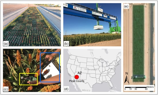
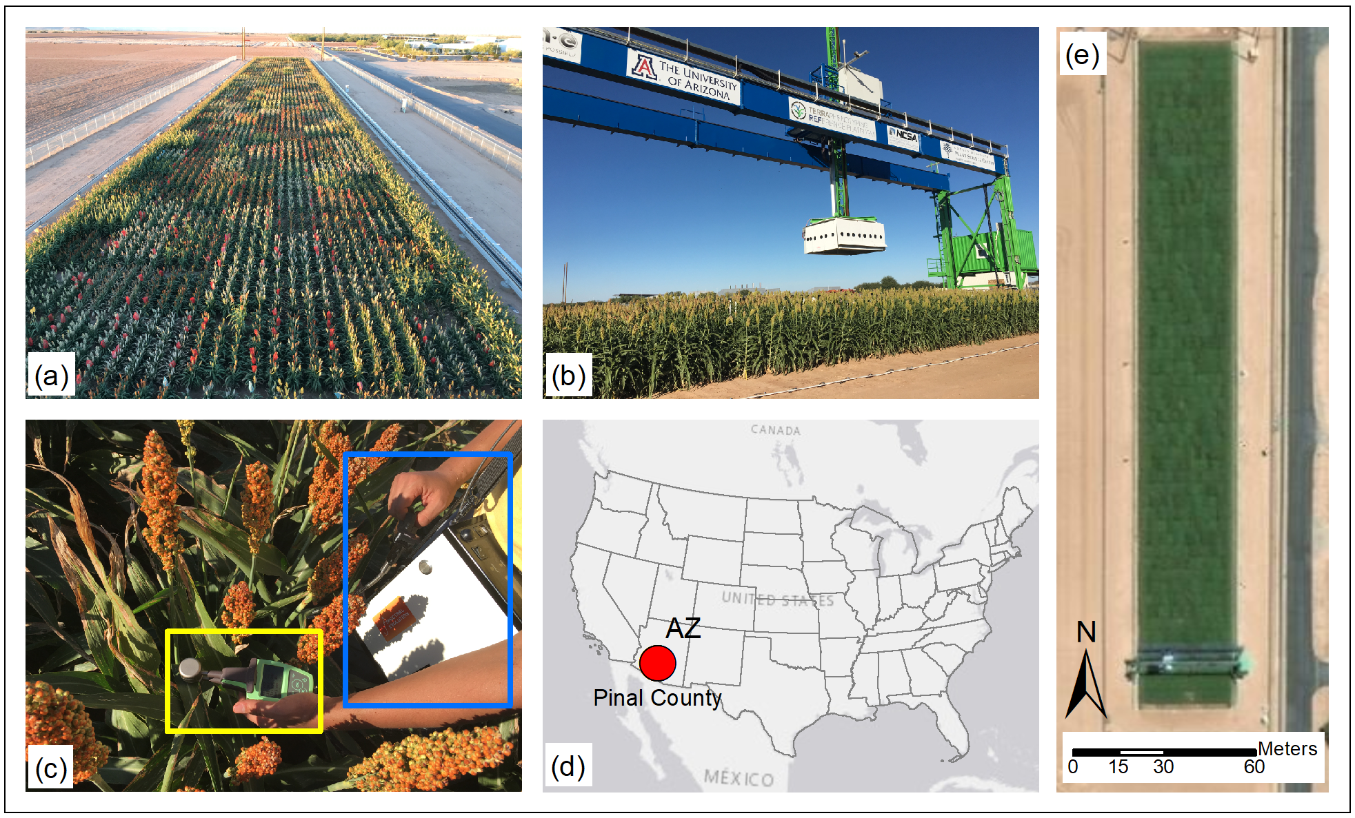
2.1. Study Site and Plant Material

The study area (Figure 1) is the Transportation Energy Resources from Renewable Agriculture Phenotyping Reference Platform (TERRA-REF) field scanner (Figure 1b) field site at the Maricopa Agricultural Center, Maricopa, Arizona, United States. The details of this field scanner system can be found in the research of Burnette et al. [65]. The experimental field site (33.070°N, 111.974°W, elevation 360 m) was planted on 3 August 2016 with two replicates of a Sorghum bicolor research population from Texas A&M (W Rooney) comprised of 173 recombinant inbred lines at the F-10 generation plus the parental lines SC56 and Tx7000. The field layout included 32 rows by 54 ranges in total, with the two outer lateral rows and end ranges as border plots to reduce edge effects. Border plots were excluded from any quantitative analysis. Experimental design followed a two-replicate alpha design with row-column constraint. Plots were four-row plots, 3.5 m long and 0.76 m row spacing, such that sorghum lines were evaluated in the two inner row subplots while the two outer rows were plot borders to reduce plot-to-plot edge effects. There were 350 total plots, where each plot had two subplots and was given unique identifiers. The field trial was managed for optimal growth. Initial irrigation was from sprinklers for emergence followed by subsurface drip lines.

2.2. Data Collection

2.2.1. Leaf Chlorophyll Concentration Measurements

In-situ ground LCC was collected using Dualex 4 Scientific (Figure 1c in yellow box, Force-A, France) handheld sensor for 394 sample leaves from 349 plots. The Dualex 4 Scientific instrument measures leaf chlorophyll index by using a red-edge band (710 nm) and a NIR band (850 nm), and estimates LCC in µg/cm² using a calibration coefficient [66]. Only sunlit representative leaves from each plot were selected for measurements. The LCC measurements were taken at noon on two days, (9 November 2016 and 11 November 2016) while the sorghum plants were at the grain development growth stage.

2.2.2. Hyperspectral Reflectance Measurements

Reflectance measures, or specifically, the hemispheric conical reflectance factor (HCRF, [67]) were collected using a Spectral Evolution portable spectroradiometer PSR-3500 (Figure 1c in blue box; Spectral Revolution, Inc., Lawrence, MA, USA) almost simultaneously with the Dualex measurements from the same sorghum leaves. Measurements were taken under clear-sky conditions near solar noon to minimize the disturbances from changes in sun angle and cloud or canopy shadow. The spectroradiometer has a spectral range of 350–2500 nm with a resolution of 3.5 nm in the 350–1000 nm range, 10 nm in the 1000–1900 nm range, and 7 nm in the 1900–2500 nm range. A reference spectrum taken from a 99% Spectralon calibration panel (Labsphere, Inc., North Sutton, NH, USA) was used to normalize leaf spectral measurements to reflectance factor. Calibration panel readings were repeated for every 15 min to readjust the baseline to account for any changes in illumination condition. A leaf clip with a bifurcated fiber-optic and a 5-watt tungsten halogen lamp light source was used to record leaf reflectance factor with a black background. With pre-configured settings, the PSR-3500 spectroradiometer averaged 40 readings automatically for each sample. The spectral reflectance factor, referred to as the reflectance hereafter, was interpolated to 1 nm, which resulted in 2151 individual spectral bands.

2.3. Fractional Derivative Calculation

Fractional-order derivative has been utilized as a tool to extract useful and sensitive information in many fields of signal processing [68,69,70]. Although fractional derivative (FD) refers to derived integer-order derivative into any positive order, the calculation of FD is complex and several algorithms exist to calculate. However, Riemann–Liouville, Grunwald–Letnikov, and Caputo are the three most frequently used classic definitions [71,72,73,74]. We adopted the Grunwald–Letnikov (G-L) definition to calculate FD at different orders in this study due to its specifically simple formula and coefficients [75]. The G-L definition is generally expressed as Equation (1):

$$d^{\alpha }f\left(x\right)=\underset{h\to 0}{\lim }\frac{1}{h^{\alpha }}{\displaystyle \sum }_{m=0}^{\left(t-a\right)/h}{\left(-1\right)}^m\frac{\mathsf{\Gamma }\left(\alpha +1\right)}{m!\mathsf{\Gamma }\left(\alpha -m+1\right)}f\left(x-mh\right)$$

(1)

where $\alpha$ is any order, $h$ is the step size, $t$ and $a$ are the upper and lower limits of the fractional order derivative, respectively. The G-L algorithm uses a Gamma function, which is expressed as $\mathsf{\Gamma }\left(\alpha \right)={{\displaystyle \int }}_0^{\infty }\exp \left(-u\right)u^{\alpha -1}du=\left(\alpha -1\right)!$. Considering the resampling interval of spectral reflectance as 1 nm and $h=1$, the derived difference in the fractional order derivative of single variable function $f\left(x\right)$ can be expressed as Equation (2):

$$\frac{d^{\alpha }f\left(x\right)}{d{x}^{\alpha }}\approx f\left(x\right)+\left(-\alpha \right)f\left(x-1\right)+\frac{\left(-\alpha \right)\left(-\alpha +1\right)}{2}f\left(x-2\right)+\dots +\frac{\mathsf{\Gamma }\left(-\alpha +1\right)}{n!\mathsf{\Gamma }\left(-\alpha +n+1\right)}f\left(x-n\right)$$

(2)

We considered calculating FD orders from 0.2 to 2.0 with 0.2 order increments. Therefore, 10 different orders were calculated from the spectral data using the G-L algorithm. A Python package named “differint” [76] was used to calculate the FD augmented spectral data.

2.4. Calculation of Vegetation Indices

Hyperspectral narrow band vegetation indices (VIs) are commonly used to estimate different crop biophysical and biochemical properties. We selected 43 common VIs (

Table 1. Vegetation indices (VIs) selected in this study for VI-based modeling.

VI	Equation	Reference
ARI1	$1/R_{550}-1/R_{700}$	[77]
ARI2	$R_{800}\left(1/R_{550}-1/R_{700}\right)$	[77]
Cart1	$R_{695}/R_{420}$	[78]
Cart2	$R_{695}/R_{760}$	[78]
Cart3	$R_{605}/R_{760}$	[78]
Cart4	$R_{710}/R_{760}$	[78]
Cart5	$R_{695}/R_{670}$	[78]
CCI	$(R_{777}-R_{747})/R_{673}$	[79]
Datt1	$(R_{850}-R_{710})/(R_{850}-R_{680})$	[80]
Datt2	$R_{850}/R_{710}$	[80]
Datt3	$R_{754}/R_{704}$	[80]
EVI	$2.5\left((R_{800}-R_{670}\right)/(R_{800}-6R_{670}-7.5R_{475}+1))$	[81,82]
GNDVI1	$(R_{750}-R_{550})/(R_{750}+R_{550})$	[83]
GNDVI2	$(R_{800}-R_{550})/(R_{800}+R_{550})$	[83]
MCARI1	$((R_{700}-R_{670})-0.2(R_{700}-R_{550}))\left(R_{700}/R_{670}\right)$	[84]
MCARI2	$1.2(2.5(R_{800}-R_{670})-1.3(R_{800}-R_{550}))$	[85]
mNDVI	$(R_{750}-R_{705})/(R_{750}+R_{705}-2R_{445})$	[80,86]
mSR	$(R_{750}-R_{445})/(R_{705}-R_{445})$	[80,86]
MTCI	$(R_{754}-R_{709})/(R_{709}-R_{681})$	[87]
MTVI1	$1.2(1.2(R_{800}-R_{550})-2.5(R_{670}-R_{550}))$	[85]
NDCI	$(R_{762}-R_{527})/(R_{762}+R_{527})$	[88]
NDVI	$(R_{750}-R_{705})/(R_{750}+R_{705})$	[89]
PRI	$(R_{531}-R_{570})/(R_{531}+R_{570})$	[90]
PSRI	$(R_{678}-R_{500})/R_{750}$	[91]
REP	$700+40\left((R_{670}-R_{780}\right)/2-R_{700}))/(R_{740}-R_{700})$	[92]
RIdb	$R_{735}/R_{720}$	[93]
SIPI	$(R_{800}-R_{445})/(R_{800}+R_{680})$	[94]
SPVI1	$0.4\times 3.7(R_{800}-R_{670})-1.2\left|R_{530}-R_{670}\right|$	[95,96]
SPVI2	$0.4\times 3.7(R_{800}-R_{670})-1.2\left|R_{550}-R_{670}\right|$	[95]
SR440/690	$R_{440}/R_{690}$	[97]
SR700/670	$R_{700}/R_{670}$	[98]
SR750/550	$R_{750}/R_{550}$	[98]
SR750/700	$R_{750}/R_{700}$	[99]
SR750/710	$R_{750}/R_{710}$	[100]
SR752/690	$R_{752}/R_{690}$	[100]
SR800/680	$R_{800}/R_{680}$	[86]
SRPI	$R_{430}/R_{680}$	[101]
TCARI	$3\left((R_{700}-R_{670}\right)-0.2(R_{700}-R_{550})(R_{700}/R_{670}))$	[18]
TCARI2	$3\left((R_{750}-R_{705}\right)-0.2(R_{750}-R_{550})(R_{750}/R_{705}))$	[20]
TVI	$0.5(120(R_{750}-R_{550})-200(R_{670}-R_{550}))$	[102]
VOG1	$R_{740}/R_{720}$	[103]
VOG2	$(R_{734}-R_{747})/(R_{715}+R_{726})$	[103]
VOG3	$(R_{734}-R_{747})/(R_{715}+R_{720})$	[103]

) based on studies that estimated different plant biochemical traits.

2.5. Feature Selection Methods

Feature selection is one of the most important pre-processing steps before performing any ML regression or classification pipeline [104,105,106]. Since hyperspectral data usually contain a large number of features (i.e., wavelengths), it is ideal to reduce the number of features by selecting the most sensitive features. Our spectral data contained reflectance values for wavelengths from 350–2500 nm with 1 nm intervals, which resulted in 2151 features. Therefore, dimensionality reduction by selecting features that were sensitive to LCC was a necessary step. Other than assessing the impact of FD in estimating LCC using different ML algorithms, we also focused on the effect of different feature selection methods and number of features within the pipeline. We used three common feature selection methods: Pearson’s correlation coefficient (PCC), partial least square based variable importance in the projection (VIP), and random forest based mean decrease impurity (MDI) to rank the importance of features.

2.5.1. Pearson’s Correlation Coefficient (PCC)

Pearson’s correlation coefficient (PCC) is a measure of the linear dependence between two random variables, which is formally defined as the covariance of the variables divided by the product of their standard deviations. The calculation of PCC ($r_{xy}$) can be expressed as Equation (3):

$$r_{xy}=\frac{{{\displaystyle \sum }}_{i=1}^n\left(x_i-\overline{x}\right){{\displaystyle \sum }}_{i=1}^n\left(y_i-\overline{y}\right)}{\sqrt{{{\displaystyle \sum }}_{i=1}^n{\left(x_i-\overline{x}\right)}^2}\sqrt{{{\displaystyle \sum }}_{i=1}^n{\left(y_i-\overline{y}\right)}^2}}$$

(3)

where $\overline{x}=\frac{1}{n}{\displaystyle \sum }_{i=1}^n{x}_i$ and $\overline{y}=\frac{1}{n}{\displaystyle \sum }_{i=1}^n{y}_i$ denote the mean of $x$ and $y$, respectively, with $n$ sample size. The coefficient ($r_{xy}$) ranges from –1 to 1 and it is invariant to linear transformations of either variables. The feature importance scores were calculated based on the absolute value of PCC.

2.5.2. Variable Importance in the Projection (VIP)

Partial least squares (PLS) regression is a common regression technique which is based on explanatory variables that have maximal covariance with the target variable. However, a key feature of PLS regression is that the importance of explanatory variables in predicting the target variable can be quantified by a metric called variable importance in the projection (VIP). The VIP score measures the explicative power of explanatory variables with respect to the target variable which is based on the PLS regression. Feature selection using VIP has been utilized in several studies related to remote sensing of vegetation [107,108,109,110]. According to Eriksson and colleagues [111], the VIP score for the $k$th variable for target variable $y$ can be computed with Equation (4):

$$VI{P}_k=\sqrt{\frac{K{{\displaystyle \sum }}_{a=1}^A\left(q_a^2{t}_a^T{t}_a\right)\left(w_{ak}/w_k{}^2\right)}{{{\displaystyle \sum }}_{a=1}^A\left(q_a^2{t}_a^T{t}_a\right)}}$$

(4)

where $a=1,2\dots ,A$, which is the number of PLS components, $K$ is the number of columns of $X$ (i.e., features or wavelengths), $w_{ak}$ is the loading weight of the $k$th variable in the $a$th component, and $t_a$, $w_a$, and $q_a$ are the $a$th column vectors of $T$, $W$, and $Q$, respectively. Here, $W$ contains the $X$-weights defining the common latent variable space $T$ relating $X$ and $y$, and $Q$ holds the loading vectors that best represent the $y$ space. The variable with a higher VIP score shows the relevancy of using that variable to predict the target variable.

2.5.3. Mean Decrease Impurity (MDI)

Random forest is an ensemble learning technique based on randomized decision trees and impurity measurements [112] that can provide different feature importance measures. One such technique is known as Gini importance or mean decrease impurity (MDI), when the random forest uses Gini index as its impurity measurement. Breiman [112] proposed to evaluate the importance of a variable $k$ for predicting $y$ (i.e., LCC) by adding up the weighted impurity decreases ($p\left(t\right)\mathsf{\Delta }i\left(s_t,t\right)$) for all nodes $t$ where $k$ is used and averaged over all $N_T$ trees in the forest as in Equation (5):

$$MD{I}_k=\frac{1}{N_T}{\displaystyle \sum }_T{\displaystyle \sum }_{t\in T:v\left(s_t\right)=k}p\left(t\right)\mathsf{\Delta }i\left(s_t,t\right)$$

(5)

where $p\left(t\right)$ is the proportion $N_t/N$ of sample reaching $t$, and $v\left(s_t\right)$ is the variable used in split $s_t$. Few studies have implemented MDI scoring for feature selection in ML pipeline [108,113,114]. In our study, the MDI score of a variable (i.e., wavelength or VI) represents the corresponding importance estimating LCC.

2.6. Machine Learning Algorithms

In the plant phenotyping community, several machine learning (ML) algorithms have become popular in terms of both accuracy and computational efficiency [115]. We investigated four commonly used ML regression techniques (i.e., PLSR, RFR, SVR, and ELR) for estimating LCC from reflectance and VI-based spectra with derivative analysis. PLSR is a multivariate calibration technique that uses component projection to reduce the full feature space to a smaller number of non-correlated features (also known as latent variables) containing the most useful information [116]. Therefore, PLSR was found to be very effective when the feature space is large, and multicollinearity exists within different features [117]. RFR is an ensemble-learning algorithm that accumulates a large set of decision trees, which are a hierarchically organized set of conditions or restrictions [118]. The process starts with fitting decision tree to randomly drawn samples and for each tree node a subset of input features is selected. Due to random selection of features in each tree, RFR is tolerant to outliers and noise [119]. SVR is the regression implementation of support vector machine (SVM). SVM transforms the non-linear regression problem to a linear one by utilizing different kernel functions. These functions then map the original input space into a high-dimensional feature space to find unique global solutions that are not exploited by multiple local minima [120]. ELR is the regression version of extreme learning machine (ELM), which is a feed-forward neural network with one input layer, one hidden layer, and one output layer [60]. ELM can provide high computational efficiency because the hidden node parameters are generated randomly [8].

2.7. Modeling Pipeline and Evaluation

An automated modeling pipeline was developd (Figure 2) to train different ML regression techniques. After creating both reflectance-based and VI-based derivative order datasets, the modeling pipeline started with dividing the dataset into training (n = 244) and validation (n = 105) sets by a 70%/30% split. The validation set was kept completely outside of the feature selection and model training parts, and only utilized during the final model evaluation step. Since different derivative orders had different ranges of reflectance values, the features were scaled from 0 to 1 before any modeling steps. Feature importance scores were calculated using three feature selection methods (i.e., PCC, VIP, and MDI). Since both VIP and MDI were required to train PLSR and RFR models first, the training parameters were selected based on a grid search algorithm and 10-fold cross-validation. Based on different feature importance scores, different groups of features were extracted from different derivative orders. For reflectance-based analysis, 25, 50, 75, 100, 125, 150, 175, and 200 feature groups were created, whereas for VI-based analysis, 5, 10, 15, 20, 25, 30, 35, and 40 feature groups were extracted. Each of these groups from different FD orders were input data for ML algorithms.

The feature groups from both reflectance-based and VI-based data were trained with different ML models. Since different models require different training parameters, we carefully selected different ranges of model parameters for PLSR, RFR, SVR, and ELR based on extensive literature survey, and applied a grid search algorithm to select the best combination of model parameters. The grid search was performed with a 10-fold cross-validation and mean squared error (MSE) was selected as the scoring criteria. Therefore, the combination of parameters resulting in the lowest MSE was considered as the optimal parameters for the model. Each feature group from different derivative orders was processed through this technique and the average MSE score for each input set was retained. Finally, the combination of feature selection method and number of features that showed the lowest MSE score within a particular derivative order and ML algorithm was used for model evaluation with the validation set. The modeling pipeline was implemented in Python and the ML algorithms were utilized from the “Scikit-learn” package [121].

The evaluation of model performance was conducted by using the coefficient of determination ($R^2$), root mean squared error ($RMSE$), and relative RMSE ($RMSE\%$). The equations are as follows:

$$R^2=1-\frac{{{\displaystyle \sum }}_{i=1}^n{\left(y_i-{\widehat{y}}_i\right)}^2}{{\left(y_i-{\overline{y}}_i\right)}^2}$$

(6)

$$RMSE=\sqrt{\frac{{{\displaystyle \sum }}_{i=1}^n{\left(y_i-{\widehat{y}}_i\right)}^2}{n-1}}$$

(7)

$$RMSE\%=\frac{RMSE}{\overline{y}}\ast 100$$

(8)

where $i=1,2,3,\dots \dots ..,n$ is the validation sample, ${\widehat{y}}_i$ and $y_i$ represent the predicted and measured LCC values, respectively, and $\overline{y}$ is the average of each measurable variable.

3. Results

3.1. Descriptive Statistics of Collected Samples

The descriptive statistics and distribution of sample LCC are presented in

Table 2. Descriptive statistics of LCC samples (µg/cm²).

	Sample Size	Maximum	Minimum	Mean	SD	CV (%)
LCC (µg/cm2)	349	70.30	30.80	50.26	7.54	15.00

Notes: SD: standard deviation; CV: coefficient of variation.

and Figure 3a, respectively. The collected leaf samples showed a range of LCC values from 30.8 to 70.3 µg/cm² with a mean value of 50.26 µg/cm². The sample distribution had a standard deviation of 7.54 with a coefficient of variation (CV) of 15%. Figure 3a also shows normally distributed LCC sample values. The descriptive statistics for spectral features are visually represented in Figure 3b. The mean spectral curve (350–2500 nm) of corresponding LCC samples shows a typical reflectance pattern of healthy vegetation: moderately strong reflectance at green region (approximately 500–650 nm), very strong reflectance at NIR region (approximately 750–1000 nm), and two water absorption regions at around 1500 nm and 2000 nm. This reveals that the sample leaves selected for this study were healthy and representative for the analysis.

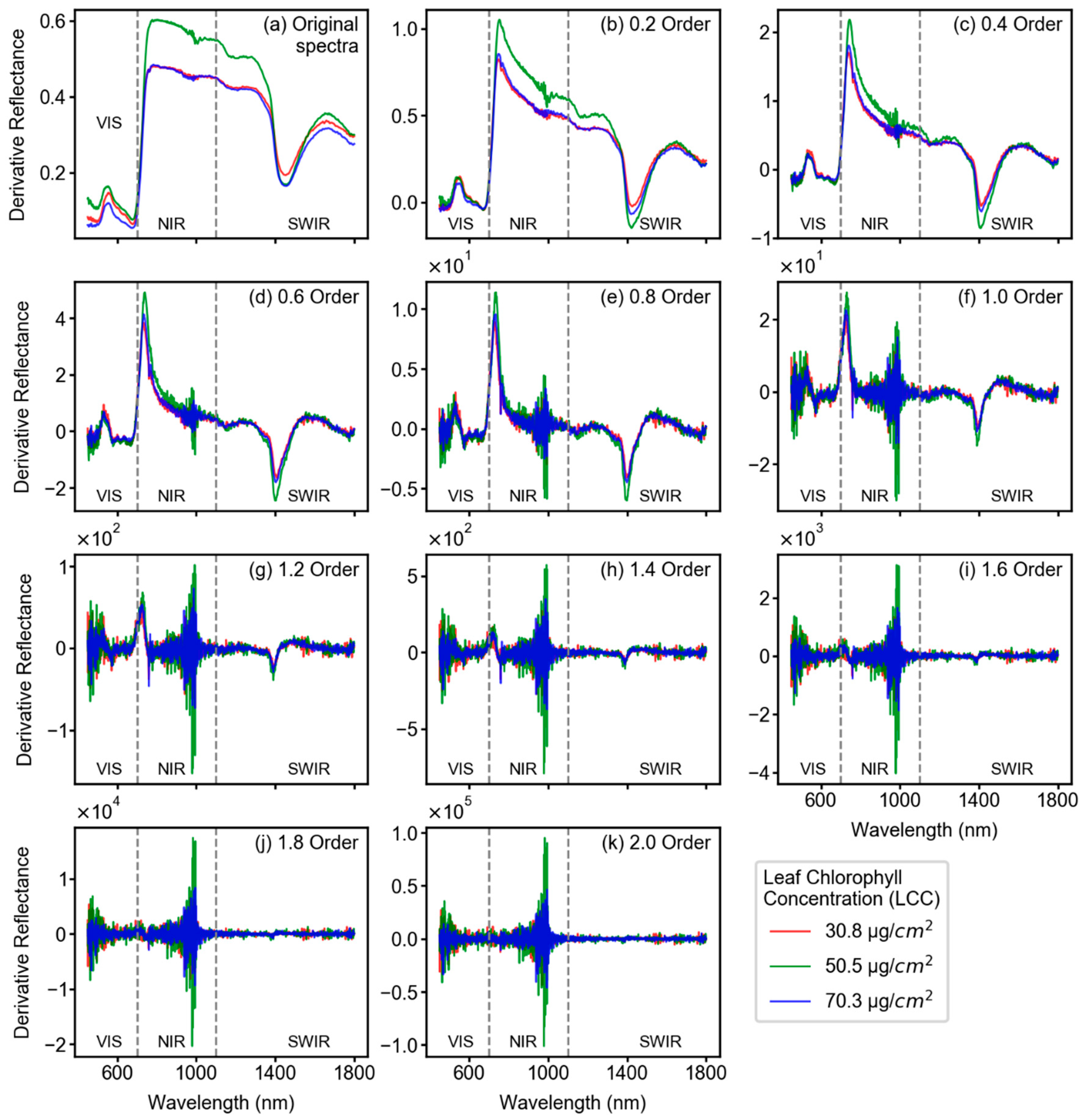
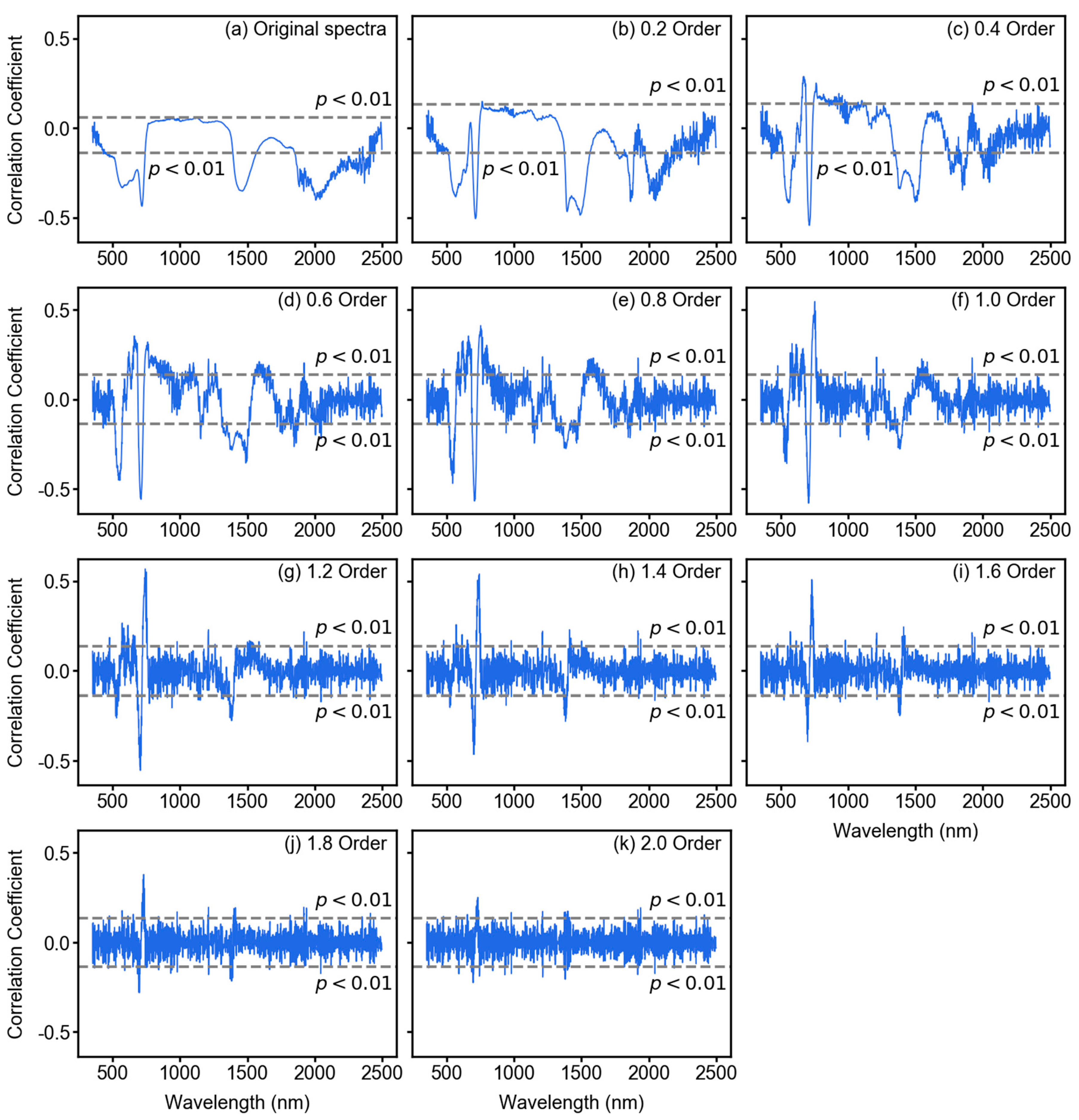
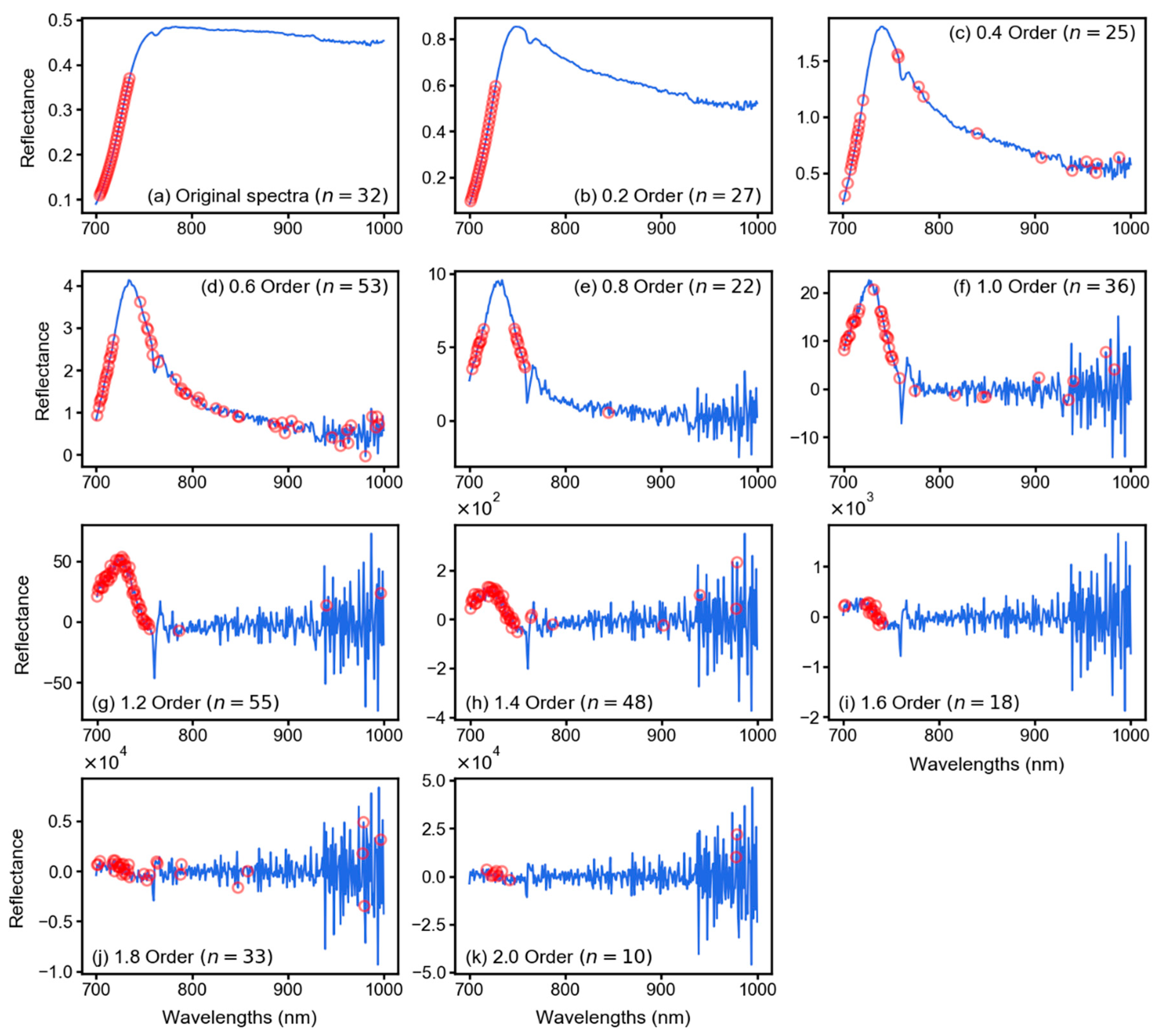
3.2. Spectral Features After Fractional Derivative Analysis

Fractional derivative-augmented spectra showed varying spectral patterns with increasing fractional orders. Figure 4 shows such pattern from the corresponding reflectance spectra of three LCC samples: the minimum (red line), maximum (green line), and median (blue line) LCC values. In the case of the original spectral reflectance factor (Figure 4a, from here on the reflectance factor will be denoted as original spectra), the maximum LCC spectra showed higher reflectance peaks at the NIR region (around 750–800 nm) compared to the other two spectra. However, the difference between these reflectance peaks at the NIR region started to diminish with fractional derivative analysis, specifically after 0.4 order (Figure 4c). Derivative treatment also led to increase in the reflectance value with increasing derivative orders exponentially, which allowed the derivative spectra to be sensitive to subtle changes in the reflectance factor.

Based on Figure 4, the number of reflectance and absorption peaks increased with incremental derivative orders compared to original spectra. For example, a subtle reflectance peak in the original spectra of maximum LCC sample (green line in Figure 4a) at around 800–1000 nm is amplified in the 0.2 derivative order spectra (Figure 4b). The FD treatment to reflectance spectra enabled sensitive features to become more significant by increasing the derivative reflectance value at certain bands (e.g., the derivative reflectance curve showed a sharp change at around 1000 nm in 0.4 order, Figure 4c), whereas the less sensitive bands were found comparatively lower in their derivative reflectance values.

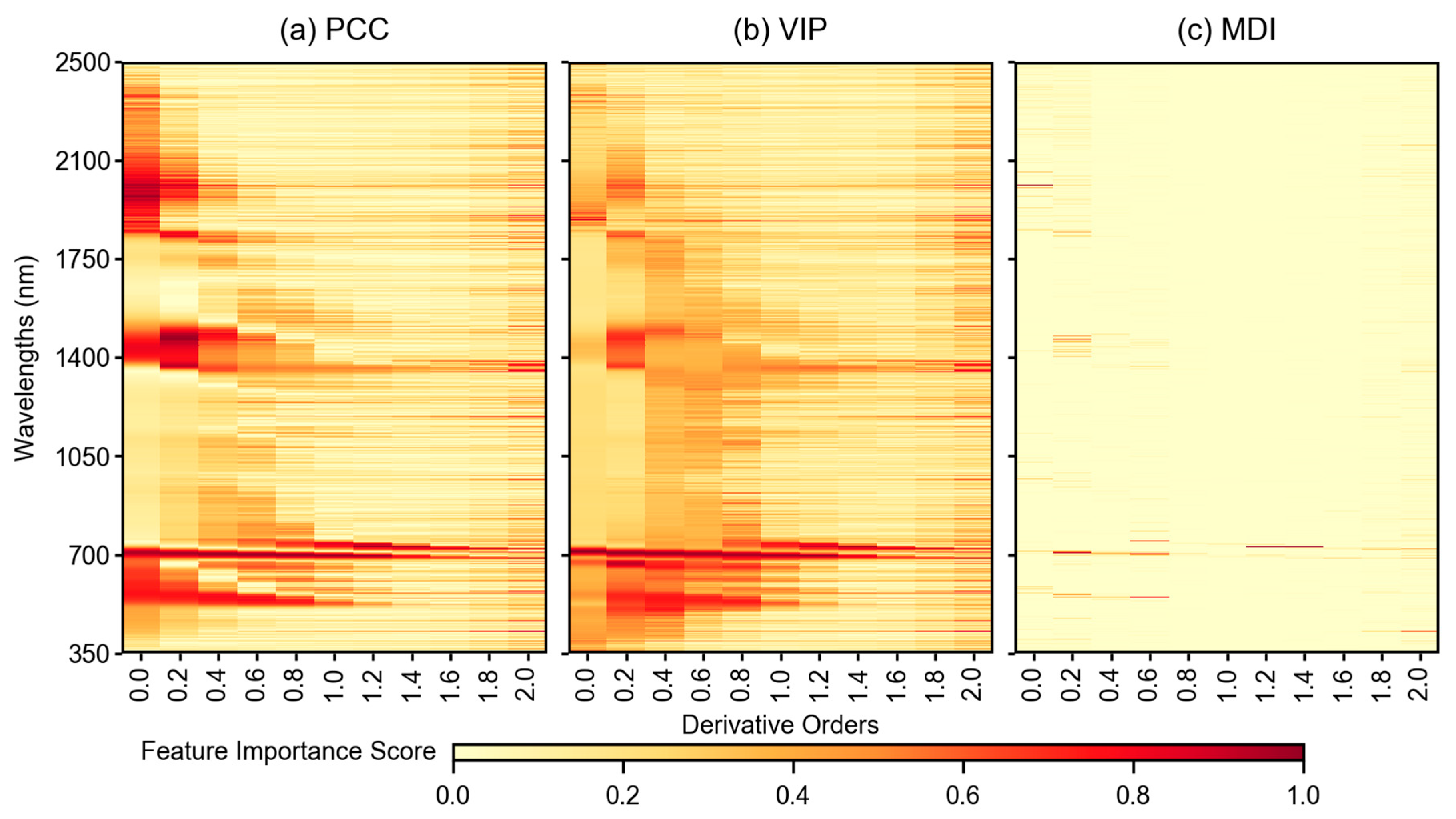
3.3. Feature Importance Scores

The relationship between different features and the target variable in this study (i.e., LCC) is a crucial step before performing model training. Figure 5 shows such a relationship between features from different derivative orders and LCC based on Pearson’s correlation coefficient (Pearson’s R). Pearson’s R ranges from –1 to +1, which represent the negative and positive relationships, respectively. All correlation coefficients from different features and LCC values were tested at the 0.01 significance level (99% confidence); they are shown in Figure 5 for each derivative order. Overall, there were negative correlations between original reflectance spectra and LCC at around 750 nm, 1400 nm, and 2000 nm wavelengths, where some features passed the significance test (Figure 5a). Very few features in original spectra showed a positive correlation and not a single feature with a positive correlation showed statistical significance (Figure 5a). However, with increasing derivative orders, both the correlation coefficient and number of features passing the significance test increased (Figure 5b–k). The highest correlation (both positive and negative) was found at around 700–750 nm range from 1.0 and 1.2 order derivatives. After 1.4 order, the overall correlation and number of significant features started dropping and the correlation curve became noisy (Figure 5i–k).

Figure 6 and Figure 7 show the feature importance scores from different feature selection methods for reflectance spectra and VIs, respectively. The PCC, VIP, and MDI scores were scaled in the range of 0–1 to make uniform comparison of scores between each derivative orders and feature selection methods. An important consideration for this analysis was that the scores were calculated using only the training samples, whereas the validation set was set aside for further model evaluations. In terms of reflectance-based feature importance scores (Figure 6), the PCC tended to extract sensitive features from around 700 nm, 1400 nm, and 1800–2400 nm range (Figure 6a). With increasing derivative orders, the most important features were concentrated at around 700 nm and 1400 nm, and after 1.6 order, the pattern of important features became noisy. The VIP scores (Figure 6b) showed a similar pattern of feature importance as the PCC, however, the values were slightly different. Alternatively, in terms of MDI (Figure 6c), the feature importance was more discrete than PCC and VIP. The MDI resulted in important features at the 2000 nm region for original spectra (order 0.0), whereas with increasing derivative orders, the important features were found at around 700–800 nm region. Usually this region is considered as the NIR region and the correlation between features at this region and LCC was found significantly improving with increasing derivative orders (Figure 5). However, the MDI highlighted unique wavelengths as a result of very clear and sharper increase in feature importance.

Feature importance scores from the VIs are shown in Figure 7. The scores are shown for all 43 features with different feature selection methods, however, the order of the features in Figure 7 does not represent any logical meaning. Similar to the reflectance-based feature importance scores, the PCC and VIP showed similar patterns of feature importance with different derivative orders. The PCC tended to highlight several important features even with original spectral data (order 0.0), for example, Cart₄, Datt₁, MTCI, NDVI, REP, RI_db, SR_750/710, VOG₂, and VOG₃ were found as showing higher scores. With increasing derivative orders, the scores for different features became noisier (Figure 7a,b). In terms of MDI (Figure 7c), very few features were highlighted in each derivative order, for example, only Vog₂ and Vog₃ were found highly important in original spectra, with order 0.2 and order 0.4, respectively. After order 1.4, the number of important features increased abruptly.

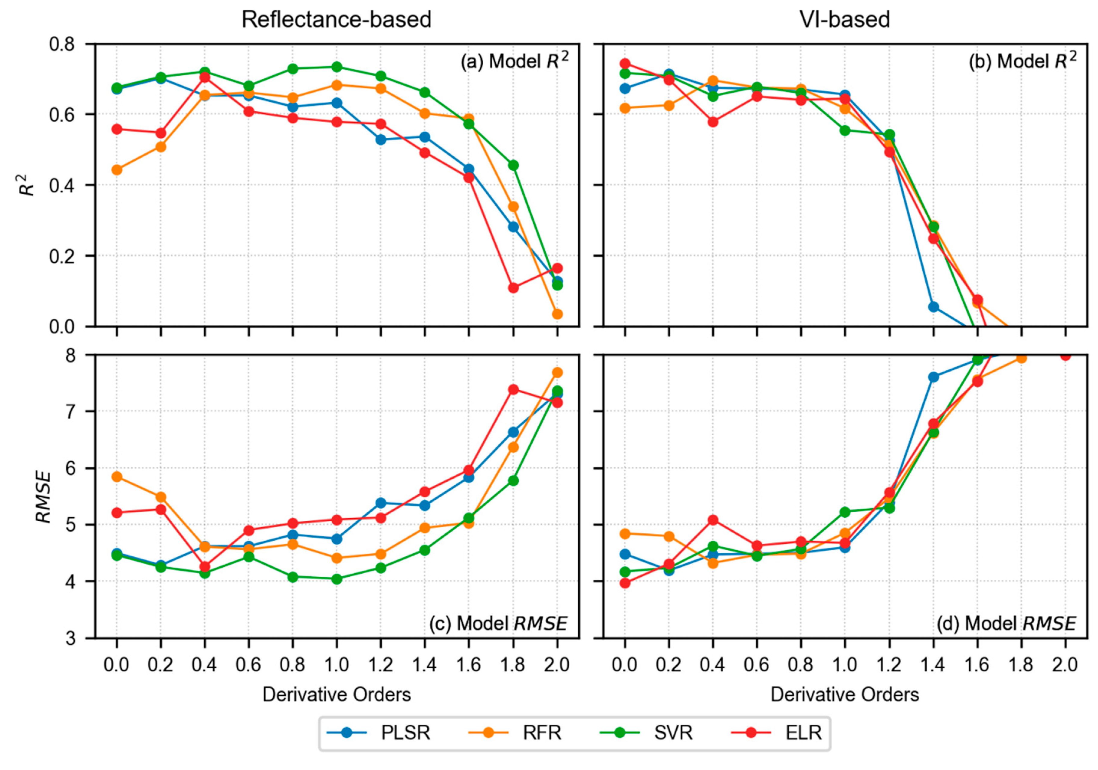
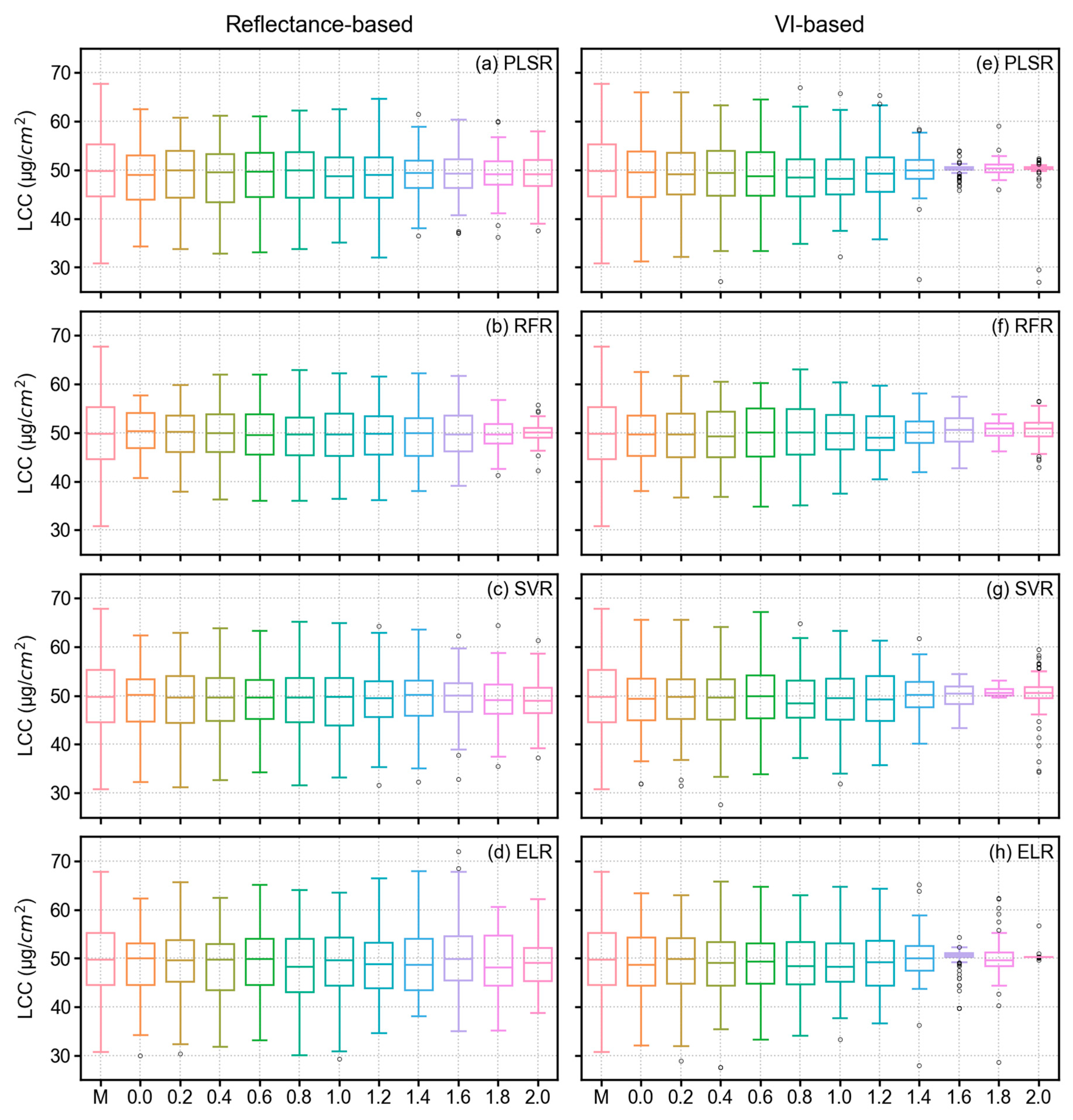
3.4. Model Results of LCC Estimation

ML models (i.e., PLSR, RFR, SVR, and ELR) were trained with every possible combination of feature selection methods and number of feature groups. Model evaluation metrics (i.e., R², RMSE, and RMSE%) were only calculated for the combination of feature selection method and number of features that yielded the lowest cross validation MSE score from the training set. These metrics were calculated with the validation dataset and all derivative orders of two different datasets: reflectance-based and VI-based spectra. The validation metrics of LCC estimation are demonstrated in

Table 3. Validation results of partial least squares regression (PLSR), random forest regression (RFR), support vector regression (SVR), and extreme learning regression (ELR) for LCC with different derivative orders.

Ord.	Metrics	Reflectance-based				VI-based
		PLSR	RFR	SVR	ELR	PLSR	RFR	SVR	ELR
0.0	R2	0.671	0.443	0.676	0.558	0.673	0.618	0.717	0.744
	RMSE	4.493	5.842	4.459	5.207	4.477	4.841	4.169	3.964
	RMSE%	9.035	11.747	8.966	10.471	9.002	9.734	8.382	7.971
	Features	VIP-75	MDI-50	VIP-75	VIP-50	VIP-30	MDI-10	PCC-25	PCC-15
0.2	R2	0.701	0.509	0.706	0.548	0.714	0.625	0.708	0.698
	RMSE	4.279	5.486	4.249	5.265	4.187	4.794	4.231	4.306
	RMSE%	8.603	11.032	8.543	10.588	8.418	9.639	8.509	8.658
	Features	VIP-75	MDI-75	VIP-175	VIP-50	PCC-10	VIP-30	PCC-15	PCC-10
0.4	R2	0.653	0.654	0.720	0.704	0.674	0.696	0.651	0.579
	RMSE	4.616	4.605	4.142	4.261	4.468	4.320	4.623	5.081
	RMSE%	9.281	9.259	8.330	8.567	8.984	8.686	9.295	10.217
	Features	VIP-25	MDI-125	MDI-100	VIP-25	PCC-20	MDI-10	PCC-15	PCC-15
0.6	R2	0.653	0.661	0.680	0.608	0.672	0.675	0.678	0.650
	RMSE	4.614	4.560	4.427	4.901	4.482	4.464	4.445	4.624
	RMSE%	9.278	9.169	8.902	9.855	9.012	8.975	8.938	9.296
	Features	VIP-50	MDI-50	MDI-175	MDI-25	PCC-15	MDI-20	VIP-15	VIP-15
0.8	R2	0.621	0.648	0.729	0.589	0.670	0.672	0.660	0.640
	RMSE	4.820	4.649	4.078	5.018	4.499	4.483	4.566	4.697
	RMSE%	9.692	9.347	8.201	10.090	9.047	9.014	9.182	9.445
	Features	VIP-200	MDI-50	MDI-25	MDI-25	PCC-15	MDI-5	PCC-10	VIP-10
1.0	R2	0.632	0.683	0.734	0.578	0.655	0.616	0.555	0.644
	RMSE	4.747	4.409	4.041	5.086	4.596	4.850	5.226	4.673
	RMSE%	9.546	8.865	8.125	10.227	9.241	9.753	10.508	9.397
	Features	VIP-200	MDI-75	MDI-75	PCC-25	PCC-10	MDI-20	PCC-20	VIP-10
1.2	R2	0.528	0.673	0.708	0.573	0.526	0.514	0.543	0.494
	RMSE	5.380	4.480	4.235	5.119	5.393	5.461	5.296	5.572
	RMSE%	10.818	9.009	8.515	10.294	10.844	10.981	10.649	11.203
	Features	VIP-175	VIP-75	VIP-150	VIP-50	MDI-5	MDI-15	MDI-5	MDI-5
1.4	R2	0.536	0.602	0.662	0.492	0.056	0.286	0.282	0.249
	RMSE	5.332	4.937	4.550	5.579	7.607	6.614	6.633	6.786
	RMSE%	10.721	9.927	9.149	11.219	15.295	13.299	13.337	13.645
	Features	VIP-200	MDI-25	PCC-150	MDI-25	VIP-15	MDI-15	MDI-5	PCC-5
1.6	R2	0.446	0.588	0.573	0.420	−0.020	0.066	−0.023	0.075
	RMSE	5.830	5.028	5.119	5.962	7.906	7.567	7.919	7.530
	RMSE%	11.724	10.110	10.294	11.988	15.898	15.215	15.924	15.141
	Features	VIP-175	PCC-25	VIP-150	PCC-50	MDI-10	MDI-10	MDI-5	MDI-5
1.8	R2	0.281	0.339	0.457	0.109	−0.065	−0.028	−0.087	−0.296
	RMSE	6.637	6.368	5.771	7.393	8.082	7.940	8.164	8.915
	RMSE%	13.347	12.805	11.605	14.865	16.251	15.966	16.417	17.926
	Features	PCC-200	MDI-25	VIP-150	MDI-25	PCC-5	MDI-25	PCC-10	VIP-10
2.0	R2	0.128	0.035	0.116	0.166	−0.280	−0.239	−0.089	−0.040
	RMSE	7.311	7.691	7.361	7.151	8.860	8.715	8.173	7.986
	RMSE%	14.701	15.465	14.802	14.380	17.816	17.525	16.434	16.058
	Features	VIP-150	MDI-75	VIP-100	VIP-50	MDI-5	MDI-10	MDI-5	VIP-30

Notes: Ord. represents derivative order; Features represent the optimum feature selection method and number of features found for corresponding model and derivative order. R²: coefficient of determination; RMSE: root mean squared error; RMSE%: relative RMSE.

. In addition, the model R² and RMSE are illustrated in Figure 8 with respect to different derivative order.

In terms of reflectance-based analysis (Figure 8a,c), the derivative order of 1.0 showed superior performance with all four models (R² ranging from 0.578 to 0.734 and RMSE% ranging from 8.125 to 10.227). The predictive performance of all models showed improvement with increasing derivative order up to a particular point. For instance, PLSR (R² of 0.701 and RMSE% of 8.603) showed the highest result at order 0.2, RFR (R² of 0.683 and RMSE% of 8.865) and SVR (R² of 0.734 and RMSE% of 8.125) yielded peaks at order 1.0, and ELR (R² of 0.704 and RMSE% of 8.567) performed the best at order 0.4. After the respective orders, each model started to decline in their performance (Figure 8a,c). Overall, the SVR showed consistently good performance until the derivative order reached 1.8 (R² ranging from 0.457 to 0.734 and RMSE% ranging from 8.125 to 11.605). Table 3 also shows the best combination of feature selection method and number of features for each model and derivative order. The best performing model within the reflectance-based analysis (i.e., SVR with order 1.0) used 75 features selected by MDI. Overall, the MDI was found as the optimal feature selection method for most of the well performed models.

Alternatively, when VIs were used as input features instead of reflectance spectra for different derivative orders, the highest performance was observed at original spectra (R² ranging from 0.618 to 0.744 and RMSE% ranging from 7.971 to 9.734). The best performing model was found with ELR at original spectra (R² of 0.744 and RMSE% of 7.971), which was even higher than the best model found with reflectance-based analysis (i.e., SVR at order 1.0 resulting in R² of 0.734 and RMSE% of 8.125). The ELR with original spectra used 15 features as input which were selected by PCC. Overall, most of the well-performing models at lower derivative orders showed PCC as an optimal feature selection method. However, according to Figure 8b, the model performance decreased with increasing derivative orders within the VI-based analysis. Therefore, the LCC estimation worked better with derivative spectra at 1.0 order when direct reflectance from wavelengths was used, whereas the original spectra showed good performance when the model inputs were VIs.

The distributions of predicted LCC values using different models, derivative orders, and feature types (i.e., reflectance-based or VI-based) with validation dataset are illustrated in Figure 9. The boxplots with different models show how different the distribution of predicted LCC values is with measured LCC values. Results showed that the reflectance-based analysis yielded good performance with increasing derivative order until approximately 1.2 order, whereas the VI-based analysis showed decreasing performance (distribution of predicted LCC values showed outliers and skewness) of models with increasing derivative order.

4. Discussion

4.1. Performance Analysis of Derivative Spectra and VIs in LCC Estimation

The derivative calculus including both integer-orders and fractional-orders, has proven to be an effective tool for analyzing spectra in many fields. Although many studies have utilized first-order and second-order derivatives in estimating vegetation spectra, very few studies have utilized fractional derivative in analyzing hyperspectral reflectance of crop leaves. To our knowledge, only one study from Chen, Li, and Tang [47] found 0.6 order spectra that resulted in superior performance in estimating nitrogen concentration of natural rubber (Hevea brasiliensis). Additionally, Wang, Zhang, Kung, and Johnson [35] reported that 1.2 order fractional derivative of hyperspectral data yielded the best results for estimating soil organic matter content. Fu, Xiong, and Tian [39] conducted a similar investigation and showed that FD analysis can increase the correlation coefficient between FD-augmented spectra and soil organic matter content. However, Fu, Xiong, and Tian [39] did not conclude with any single order that provided the best result in predictive analytics. The results from our study also dictate that when reflectance spectra are used in modeling LCC, derivative calculus can significantly increase the correlation between LCC until a certain order (Figure 5). However, different models yielded their best performance at different orders. For example, both SVR and RFR had higher model performance at order 1.0, but PLSR showed its best performance at order 0.2. We also found that the best performance was retrieved from 1.0 order (i.e., first order) with SVR model when reflectance spectra were used as model input. However, the second highest model performance from 0.8 order with SVR (R² of 0.729 and RMSE% of 8.201) used fewer features (n = 25) compared to the highest performing model that used more features (n = 75), yet the results were only slightly less than the best model. Therefore, we find it inconclusive to state that either fractional derivative or integer-order derivative is better in estimating LCC from sorghum.

Derivative calculus augmented spectra have the capability to extract more useful information from hyperspectral data since the order is extended arbitrarily to non-integers as well as integers [29,30,34]. This process increases the possibility of highlighting more detailed features within the limits of integer derivatives. For example, Figure 10 shows reflectance spectra of a sample leaf (i.e., from the median LCC value of 50.5 µg/cm²) without any derivative analysis (i.e., original spectrum, Figure 10a) and derivative spectrum from order 0.2 to 2.0 with a smaller spectral window (i.e., the NIR region of 700–1000 nm). The selected features with the best models found at each derivative order are also highlighted. Figure 10 is a close-up version of Figure 4 that highlights how the increasing derivative order amplify certain information in the spectral curve and how important features are then selected by different feature selection methods. According to Figure 10a, the original spectra show an increasing slope until around 760 nm and start to flatten out until 1000 nm. With increasing derivative order, the flatten curve starts to show abrupt peaks on it and the important features start to appear in a distributed manner. For example, with order 0.6 (Figure 10d), important features are seen all over the spectrum instead of clustering at the lower end of the spectrum as in the case of original spectra (Figure 10a). This is the reason that the correlation coefficient between LCC and derivative spectra significantly increased with increasing derivative orders (Figure 5).

Alternatively, use of VIs has been considered as a convenient and powerful feature for estimating different plant characteristics from spectral data. Many studies have reported the good predictive capabilities of using VIs in predicting leaf biochemical properties [122,123,124,125,126,127,128]. We have also found superior results with VIs instead of performing any derivative augmentation (i.e., the best performing model was from 15 VIs). Figure 11 shows those VIs that resulted in the best performing model using ELR and original spectra. These VIs were selected by PCC as the feature selection method. One possible reason behind VIs showing the best performance could be that VIs were developed to enhance certain vegetation information. LCC is considered as one of the major leaf pigments that reflects the photosynthetic ability and overall health status of a plant [129]. Although the VIs selected for this study were based on a wide literature survey, most of the VIs were found highly sensitive to LCC. For example, the highest correlation was found for the Red-Edge Position (REP) index (Figure 11, equation in Table 1) developed by Clevers [92]. This index highlights reflectance from the red-edge position of the spectrum and simplifies the spectral curve to a straight line between 700 nm and 740 nm. The reflectance of the REP was then estimated as being half of the reflectance in the NIR at about 780 nm and the reflectance minimum of the chlorophyll absorption feature at around 670 nm. By highlighting the chlorophyll absorption band, this index provided the best score and can be used as a potential feature. Other VIs were also closely related to LCC and other leaf biochemical parameters which helped different models to estimate LCC using the original spectra instead of using VIs from derivative transformed spectra. An advantage of using VIs instead of reflectance is that they reduce the feature space and increase model computational efficiency. However, the selection of VIs is very important for estimating certain plant characteristics.

4.2. Impact of Feature Selection Methods in Modeling Pipeline

Selecting sensitive features for modeling any biochemical properties is crucial, especially when the input feature space is large. Use of PCC (or absolute value of Pearson’s correlation coefficient) is very common for sensitive feature selection in the plant science community. However, we also explored the effectiveness of the VIP score from PLSR and MDI score from RFR. Results suggested that in terms of reflectance-based analysis, MDI worked better since the scores were not saturated over the spectrum for different derivative orders. MDI score is calculated based on node impurity, which is a measure of homogeneity of the variable. With increasing order, the difference between each feature range increases a lot with abrupt changes which increases the impurity in the feature space. That is why MDI can unilaterally pick important features from the spectrum at large distances with increasing orders. With PCC, there exists the chance of multicollinearity (correlation among features) which results in similar feature importance score for adjacent bands in our analysis. On the other hand, since MDI is a tree-based scoring measure, the multicollinearity problem was avoided.

On the other hand, in terms of VI-based analysis, PCC tends to pick up sensitive features distributed over all the available VIs. Since some of the individual VIs showed higher correlation compared to individual original spectra or derivative augmented spectra, PCC was able to pick up important features for modeling. An advantage of PCC is that it does not need to train any model, whereas both VIP and MDI scores were calculated after training PLSR and RFR models, respectively.

4.3. Performance of Machine Learning Models in LCC Estimation

In plant science and remote sensing communities, the PLSR, RFR, and SVR have proven to be effective machine learning models for estimating biochemical properties. Recently, ELR has been utilized as a potential machine learning method in regression problems due to its enhanced computational efficiency [58,63]. Our study reveals that within reflectance-based analysis, SVR consistently outperformed all other models in every FD order. Many studies have also reported the superior predictive capability of SVR in estimating crop phenotypic traits [130,131,132]. This can be attributed to the high generalization ability of SVR by providing a global minimum solution [131,133]. ELR also performed well at 0.4 order derivatives but started to decrease its performance with increasing derivative order. Although the difference between model evaluation metrics of different orders is small in some cases (e.g., SVR at order 1.0 and SVR at order 0.8), it has to be noted that the model training was performed with a 10-fold cross validation and the evaluation metrics were calculated using a validation dataset which was completely independent of the training dataset and only used for model evaluation. This showed the robustness of the trained models. Arguably, our study concluded that SVR from order 1.0 is better than SVR from order 0.8. However, for future studies with other crops or other study areas, the result may vary, so careful design of the modeling pipeline is required before making such an inference.

In terms of VI-based analysis, most of the model performed well with original spectra. The best performing model within both VI-based and reflectance-based analysis was found with ELR from reflectance. However, the ML models in terms of VI-based analysis did not perform well with increasing derivative orders. The reason behind this is that VIs were developed to amplify certain information from vegetation spectra rather than derivative-augmented spectra. Therefore, the derivative-augmented spectra were already amplified with different orders and when VIs were calculated from these derivative-augmented spectra, more noise was introduced to the feature space. This resulted in continuous poor performance of models over increasing FD orders. Therefore, it is not advisable to calculate VIs from derivative-augmented spectra.

5. Conclusions

Accurate and non-destructive measures for estimating LCC for sorghum is an important step to support plant breeders and genetic selection studies. This study investigates the effectiveness of derivative calculus and machine learning models in estimating LCC of sorghum from hyperspectral spectroscopy. Major conclusions include:

• In terms of reflectance-based analysis, increasing derivative order can show improved model performance until a certain order; however, it is inconclusive to state that a particular derivative order is optimal for estimating LCC of sorghum. Further assessment with data from multiple study sites and growth stages is required to make such an inference.
• VI-based modeling with original spectra outperformed reflectance-based modeling with derivative-augmented spectra.
• Sensitive feature selection is a crucial step in any machine learning pipeline. MDI score was found effective in selecting sensitive features from a large feature space (reflectance-based analysis), whereas PCC worked better with a smaller feature space (VI-based analysis).
• When single wavelengths were used in the analysis from different FD orders, SVR outperformed all other models. However, PLSR and ELR required fewer model parameters and computational time, which can be advantageous in model training. Alternatively, ELR with VIs from original spectra yielded slightly better results compared to all other models. Therefore, ELR worked better when hand-crafted features (VIs) were used.

The findings from this study will help plant breeders and scientists in estimating LCC for sorghum non-destructively and efficiently. It also demonstrates a potential framework for how to prepare a semi-automated machine learning pipeline that highlights robust data processing, feature selection, model training, and model evaluation techniques, which can be adopted to other plant phenotypic estimation studies as well. Our next steps and future work will include data augmentation and transferring the pipeline to hyperspectral imagery collected from unmanned aerial vehicle platforms to estimate LCC and other biochemical properties of sorghum.

References

1. Stringer, R. Food Security Global Overview. In Food Poverty and Insecurity: International Food Inequalities; Caraher, M., Coveney, J., Eds.; Springer International Publishing: Cham, Switzerland, 2016; pp. 11–18. [Google Scholar]
2. Myers, S.S.; Smith, M.R.; Guth, S.; Golden, C.D.; Vaitla, B.; Mueller, N.D.; Dangour, A.D.; Huybers, P. Climate Change and Global Food Systems: Potential Impacts on Food Security and Undernutrition. Annu. Rev. Publ. Health 2017, 38, 259–277. [Google Scholar] [CrossRef] [PubMed]
3. Stephens, E.C.; Jones, A.D.; Parsons, D. Agricultural systems research and global food security in the 21st century: An overview and roadmap for future opportunities. Agric. Syst. 2018, 163, 1–6. [Google Scholar] [CrossRef]
4. FAO; IFAD; WFP. The State of Food Insecurity in the World: Strengthening the Enabling Environment for Food Security and Nutrition; Food and Agriculture Organization of the United Nations: Rome, Italy, 2014; p. 57. [Google Scholar]
5. Monk, R.; Franks, C.; Dahlberg, J. Sorghum. In Yield Gains in Major U.S. Field Crops; Smith, S., Diers, B., Specht, J., Carver, B., Eds.; Wiley: Hoboken, NJ, USA, 2014; pp. 293–310. [Google Scholar]
6. Hadebe, S.T.; Modi, A.T.; Mabhaudhi, T. Drought Tolerance and Water Use of Cereal Crops: A Focus on Sorghum as a Food Security Crop in Sub-Saharan Africa. J. Agric. Crop. Sci 2017, 203, 177–191. [Google Scholar] [CrossRef]
7. Morris, G.P.; Ramu, P.; Deshpande, S.P.; Hash, C.T.; Shah, T.; Upadhyaya, H.D.; Riera-Lizarazu, O.; Brown, P.J.; Acharya, C.B.; Mitchell, S.E.; et al. Population genomic and genome-wide association studies of agroclimatic traits in sorghum. Proc. Natl. Acad. Sci. USA 2013, 110, 453–458. [Google Scholar] [CrossRef] [Green Version]
8. Maimaitijiang, M.; Ghulam, A.; Sidike, P.; Hartling, S.; Maimaitiyiming, M.; Peterson, K.; Shavers, E.; Fishman, J.; Peterson, J.; Kadam, S.; et al. Unmanned Aerial System (UAS)-based phenotyping of soybean using multi-sensor data fusion and extreme learning machine. ISPRS J. Photogramm. Remote Sens. 2017, 134, 43–58. [Google Scholar] [CrossRef]
9. Furbank, R.T.; Tester, M. Phenomics—Technologies to relieve the phenotyping bottleneck. Trends Plant. Sci. 2011, 16, 635–644. [Google Scholar] [CrossRef] [PubMed]
10. Chapman, S.C.; Merz, T.; Chan, A.; Jackway, P.; Hrabar, S.; Dreccer, M.F.; Holland, E.; Zheng, B.; Ling, T.J.; Jimenez-Berni, J. Pheno-Copter: A Low-Altitude, Autonomous Remote-Sensing Robotic Helicopter for High-Throughput Field-Based Phenotyping. Agronomy 2014, 4, 279–301. [Google Scholar] [CrossRef] [Green Version]
11. Watanabe, K.; Guo, W.; Arai, K.; Takanashi, H.; Kajiya-Kanegae, H.; Kobayashi, M.; Yano, K.; Tokunaga, T.; Fujiwara, T.; Tsutsumi, N.; et al. High-Throughput Phenotyping of Sorghum Plant Height Using an Unmanned Aerial Vehicle and Its Application to Genomic Prediction Modeling. Front. Plant Sci. 2017, 8. [Google Scholar] [CrossRef] [Green Version]
12. Malenovsky, Z.; Homolova, L.; Zurita-Milla, R.; Lukes, P.; Kaplan, V.; Hanus, J.; Gastellu-Etchegorry, J.P.; Schaepman, M.E. Retrieval of spruce leaf chlorophyll content from airborne image data using continuum removal and radiative transfer. Remote Sens. Environ. 2013, 131, 85–102. [Google Scholar] [CrossRef] [Green Version]
13. Houborg, R.; Fisher, J.B.; Skidmore, A.K. Advances in remote sensing of vegetation function and traits. Int. J. Appl. Earth Obs. 2015, 43, 1–6. [Google Scholar] [CrossRef] [Green Version]
14. Sun, J.; Yang, J.; Shi, S.; Chen, B.W.; Du, L.; Gong, W.; Song, S.L. Estimating Rice Leaf Nitrogen Concentration: Influence of Regression Algorithms Based on Passive and Active Leaf Reflectance. Remote Sens. 2017, 9, 951. [Google Scholar] [CrossRef] [Green Version]
15. Curran, P.J.; Dungan, J.L.; Peterson, D.L. Estimating the foliar biochemical concentration of leaves with reflectance spectrometry testing the Kokaly and Clark methodologies. Remote Sens. Environ. 2001, 76, 349–359. [Google Scholar] [CrossRef]
16. Blackburn, G.A. Hyperspectral remote sensing of plant pigments. J. Exp. Bot. 2007, 58, 855–867. [Google Scholar] [CrossRef] [PubMed] [Green Version]
17. Golhani, K.; Balasundram, S.K.; Vadamalai, G.; Pradhan, B. Estimating chlorophyll content at leaf scale in viroid-inoculated oil palm seedlings (Elaeis guineensis Jacq.) using reflectance spectra (400 nm–1050 nm). Int. J. Remote Sens. 2019, 40, 7647–7662. [Google Scholar] [CrossRef]
18. Haboudane, D.; Miller, J.R.; Tremblay, N.; Zarco-Tejada, P.J.; Dextraze, L. Integrated narrow-band vegetation indices for prediction of crop chlorophyll content for application to precision agriculture. Remote Sens. Environ. 2002, 81, 416–426. [Google Scholar] [CrossRef]
19. Gitelson, A.A.; Vina, A.; Ciganda, V.; Rundquist, D.C.; Arkebauer, T.J. Remote estimation of canopy chlorophyll content in crops. Geophys. Res. Lett. 2005, 32. [Google Scholar] [CrossRef] [Green Version]
20. Wu, C.Y.; Niu, Z.; Tang, Q.; Huang, W.J. Estimating chlorophyll content from hyperspectral vegetation indices: Modeling and validation. Agric. For. Meteorol. 2008, 148, 1230–1241. [Google Scholar] [CrossRef]
21. Croft, H.; Chen, J.M.; Zhang, Y. The applicability of empirical vegetation indices for determining leaf chlorophyll content over different leaf and canopy structures. Ecol. Complex. 2014, 17, 119–130. [Google Scholar] [CrossRef]
22. Meroni, M.; Colombo, R.; Panigada, C. Inversion of a radiative transfer model with hyperspectral observations for LAI mapping in poplar plantations. Remote Sens. Environ. 2004, 92, 195–206. [Google Scholar] [CrossRef]
23. Weiss, M.; Baret, F. Evaluation of canopy biophysical variable retrieval performances from the accumulation of large swath satellite data. Remote Sens. Environ. 1999, 70, 293–306. [Google Scholar] [CrossRef]
24. Atzberger, C. Object-based retrieval of biophysical canopy variables using artificial neural nets and radiative transfer models. Remote Sens. Environ. 2004, 93, 53–67. [Google Scholar] [CrossRef]
25. Tsai, F.; Philpot, W.D. A derivative-aided hyperspectral image analysis system for land-cover classification. IEEE Trans. Geosci. Remote 2002, 40, 416–425. [Google Scholar] [CrossRef]
26. Stavroulakis, P.; Liatsis, P.; Tipping, N.; Craddock, P. Evaluation and Optimization of the Savitzky-Golay Smoothing Filter for Noise Reduction in Thin Film Interference Signal Analysis; SPIE: Bellingham, WA, USA, 2013; Volume 8842. [Google Scholar]
27. Shafri, H.; Shafri, M.; Rozni, M.; Yusof, R. Trends and Issues in Noise Reduction for Hyperspectral Vegetation Reflectance Spectra. Eur. J. Sci. Res. 2009, 29, 404–410. [Google Scholar]
28. Han, L.H. Estimating chlorophyll-a concentration using first-derivative spectra in coastal water. Int. J. Remote Sens. 2005, 26, 5235–5244. [Google Scholar] [CrossRef]
29. Wiggins, K.; Palmer, R.; Hutchinson, W.; Drummond, P. An investigation into the use of calculating the first derivative of absorbance spectra as a tool for forensic fibre analysis. Sci. Justice 2007, 47, 9–18. [Google Scholar] [CrossRef]
30. Zhang, X.; He, Y.; Wang, C.; Xu, F.; Li, X.; Tan, C.; Chen, D.; Wang, G.; Shi, L. Estimation of Corn Canopy Chlorophyll Content Using Derivative Spectra in the O2–A Absorption Band. Front. Plant Sci. 2019, 10. [Google Scholar] [CrossRef] [Green Version]
31. Holden, H.; LeDrew, E. Accuracy Assessment of Hyperspectral Classification of Coral Reef Features. Geocarto Int. 2000, 15, 7–14. [Google Scholar] [CrossRef]
32. Pu, Y.F.; Wang, W.X.; Zhou, J.L.; Wang, Y.Y.; Jia, H.D. Fractional differential approach to detecting textural features of digital image and its fractional differential filter implementation. Sci. Chin. Ser. 2008, 51, 1319–1339. [Google Scholar] [CrossRef]
33. Wang, X.P.; Zhang, F.; Ding, J.L.; Kung, H.T.; Latif, A.; Johnson, V.C. Estimation of soil salt content (SSC) in the Ebinur Lake Wetland National Nature Reserve (ELWNNR), Northwest China, based on a Bootstrap-BP neural network model and optimal spectral indices. Sci. Total Environ. 2018, 615, 918–930. [Google Scholar] [CrossRef]
34. Kharintsev, S.S.; Salakhov, M.K. A simple method to extract spectral parameters using fractional derivative spectrometry. Spectrochim. Acta 2004, 60, 2125–2133. [Google Scholar] [CrossRef] [PubMed]
35. Wang, X.P.; Zhang, F.; Kung, H.T.; Johnson, V.C. New methods for improving the remote sensing estimation of soil organic matter content (SOMC) in the Ebinur Lake Wetland National Nature Reserve (ELWNNR) in northwest China. Remote Sens. Environ. 2018, 218, 104–118. [Google Scholar] [CrossRef]
36. Cao, H.F.; Zhang, R.X.; Yan, F.L. Spread spectrum communication and its circuit implementation using fractional-order chaotic system via a single driving variable. Commun. Nonlinear Sci. 2013, 18, 341–350. [Google Scholar] [CrossRef]
37. Duong, P.L.T.; Lee, M. Optimal design of fractional order linear system with stochastic inputs/parametric uncertainties by hybrid spectral method. J. Process. Contr. 2014, 24, 1639–1645. [Google Scholar] [CrossRef] [Green Version]
38. Huang, X.; Sun, T.T.; Li, Y.X.; Liang, J.L. A Color Image Encryption Algorithm Based on a Fractional-Order Hyperchaotic System. Entropy 2015, 17, 28–38. [Google Scholar] [CrossRef]
39. Fu, C.B.; Xiong, H.G.; Tian, A.H. Study on the Effect of Fractional Derivative on the Hyperspectral Data of Soil Organic Matter Content in Arid Region. J. Spectrosc. 2019, 7159317. [Google Scholar] [CrossRef] [Green Version]
40. Dariusz, W.B. Comparison of Fractional Order Derivatives Computational Accuracy—Right Hand vs Left Hand Definition. Appl. Math. Nonlinear Sci. 2017, 2, 237–248. [Google Scholar]
41. Schmitt, J.M. Fractional derivative analysis of diffuse reflectance spectra. Appl. Spectrosc. 1998, 52, 840–846. [Google Scholar] [CrossRef]
42. Li, Y.-l.; Tang, H.-q.; Chen, H.-x. Fractional-order derivative spectroscopy for resolving simulated overlapped Lorenztian peaks. Chemometr. Intell. Lab. 2011, 107, 83–89. [Google Scholar] [CrossRef]
43. Tong, P.J.; Du, Y.P.; Zheng, K.Y.; Wu, T.; Wang, J.J. Improvement of NIR model by fractional order Savitzky-Golay derivation (FOSGD) coupled with wavelength selection. Chemometr. Intell. Lab. 2015, 143, 40–48. [Google Scholar] [CrossRef]
44. Wang, J.; Tashpolat, T.; Ding, J.; Zhang, D.; Liu, W. Estimation of desert soil organic carbon content based on hyperspectral data preprocessing with fractional differential. Trans. Chin. Soc. Agric. Eng. 2016, 32, 161–169. [Google Scholar]
45. Xia, N.; Tiyip, T.; Kelimu, A.; Nurmemet, I.; Ding, J.L.; Zhang, F.; Zhang, D. Influence of Fractional Differential on Correlation Coefficient between EC1:5 and Reflectance Spectra of Saline Soil. J. Spectrosc. 2017. [Google Scholar] [CrossRef] [Green Version]
46. Wang, J.; Tashpolat, T.; Zhang, D. Spectral Detection of Chromium Content in Desert Soil Based on Fractional Differential. Trans. Chin. Soc. Agric. Mach. 2017, 48, 152–158. [Google Scholar] [CrossRef]
47. Chen, K.; Li, C.; Tang, R. Estimation of the nitrogen concentration of rubber tree using fractional calculus augmented NIR spectra. Ind. Crop. Prod. 2017, 108, 831–839. [Google Scholar] [CrossRef]
48. Abulaiti, Y.; Sawut, M.; Maimaitiaili, B.; Chunyue, M. A possible fractional order derivative and optimized spectral indices for assessing total nitrogen content in cotton. Comput. Electron. Agric. 2020, 171, 105275. [Google Scholar] [CrossRef]
49. Xia, Z.Z.; Yang, J.; Wang, J.; Wang, S.P.; Liu, Y. Optimizing Rice Near-Infrared Models Using Fractional Order Savitzky-Golay Derivation (FOSGD) Combined with Competitive Adaptive Reweighted Sampling (CARS). Appl. Spectrosc. 2020. [Google Scholar] [CrossRef]
50. Chen, L.; Huang, J.F.; Wang, F.M.; Tang, Y.L. Comparison between back propagation neural network and regression models for the estimation of pigment content in rice leaves and panicles using hyperspectral data. Int. J. Remote Sens. 2007, 28, 3457–3478. [Google Scholar] [CrossRef]
51. Darvishzadeh, R.; Skidmore, A.; Schlerf, M.; Atzberger, C.; Corsi, F.; Cho, M. LAI and chlorophyll estimation for a heterogeneous grassland using hyperspectral measurements. ISPRS J. Photogramm. Remote Sens. 2008, 63, 409–426. [Google Scholar] [CrossRef]
52. Singh, S.K.; Hoyos-Villegas, V.; Ray, J.D.; Smith, J.R.; Fritschi, F.B. Quantification of leaf pigments in soybean (Glycine max (L.) Merr.) based on wavelet decomposition of hyperspectral features. Field Crop. Res. 2013, 149, 20–32. [Google Scholar] [CrossRef]
53. Yi, Q.X.; Jiapaer, G.; Chen, J.M.; Bao, A.M.; Wang, F.M. Different units of measurement of carotenoids estimation in cotton using hyperspectral indices and partial least square regression. ISPRS J. Photogramm. Remote Sens. 2014, 91, 72–84. [Google Scholar] [CrossRef]
54. Zhai, Y.F.; Cui, L.J.; Zhou, X.; Gao, Y.; Fei, T.; Gao, W.X. Estimation of nitrogen, phosphorus, and potassium contents in the leaves of different plants using laboratory-based visible and near-infrared reflectance spectroscopy: Comparison of partial least-square regression and support vector machine regression methods. Int. J. Remote Sens. 2013, 34, 2502–2518. [Google Scholar] [CrossRef]
55. Kira, O.; Linker, R.; Gitelson, A. Non-destructive estimation of foliar chlorophyll and carotenoid contents: Focus on informative spectral bands. Int. J. Appl. Earth Obs. 2015, 38, 251–260. [Google Scholar] [CrossRef]
56. He, Y.; Zhang, C.; Liu, F.; Kong, W.W.; Cui, P.; Zhou, W.J.; Huang, L.X. Determination of Pigments Concentration of Oilseed Rape (Brassica Napus L.) Leaves Using Hyperspectral Imaging. Appl. Eng. Agric. 2015, 31, 23–30. [Google Scholar] [CrossRef]
57. Ge, Y.F.; Atefi, A.; Zhang, H.C.; Miao, C.Y.; Ramamurthy, R.K.; Sigmon, B.; Yang, J.L.; Schnable, J.C. High-throughput analysis of leaf physiological and chemical traits with VIS-NIR-SWIR spectroscopy: A case study with a maize diversity panel. Plant. Methods 2019, 15. [Google Scholar] [CrossRef] [PubMed] [Green Version]
58. Sonobe, R.; Sano, T.; Horie, H. Using spectral reflectance to estimate leaf chlorophyll content of tea with shading treatments. Biosyst. Eng. 2018, 175, 168–182. [Google Scholar] [CrossRef]
59. Shah, S.H.; Angel, Y.; Houborg, R.; Ali, S.; McCabe, M.F. A Random Forest Machine Learning Approach for the Retrieval of Leaf Chlorophyll Content in Wheat. Remote Sens. 2019, 11, 920. [Google Scholar] [CrossRef] [Green Version]
60. Huang, G.B.; Zhu, Q.Y.; Siew, C.K. Extreme learning machine: Theory and applications. Neurocomputing 2006, 70, 489–501. [Google Scholar] [CrossRef]
61. Chen, Y.; Yao, E.Y.; Basu, A. A 128-Channel Extreme Learning Machine-Based Neural Decoder for Brain Machine Interfaces. IEEE Trans. Biomed. Circ. Syst. 2016, 10, 679–692. [Google Scholar] [CrossRef]
62. Sidike, P.; Krieger, E.; Alom, M.Z.; Asari, V.K.; Taha, T. A fast single-image super-resolution via directional edge-guided regularized extreme learning regression. Signal. Image Video 2017, 11, 961–968. [Google Scholar] [CrossRef]
63. Maimaitiyiming, M.; Sagan, V.; Sidike, P.; Kwasniewski, M.T. Dual Activation Function-Based Extreme Learning Machine (ELM) for Estimating Grapevine Berry Yield and Quality. Remote Sens. 2019, 11, 740. [Google Scholar] [CrossRef] [Green Version]
64. Maimaitijiang, M.; Sagan, V.; Sidike, P.; Daloye, M.A.; Erkbol, H.; Fritschi, B.F. Crop Monitoring Using Satellite/UAV Data Fusion and Machine Learning. Remote Sens. 2020, 12, 1357. [Google Scholar] [CrossRef]
65. Burnette, M.; Kooper, R.; Maloney, J.D.; Rohde, G.S.; Terstriep, J.A.; Willis, C.; Fahlgren, N.; Mockler, T.; Newcomb, M.; Sagan, V.; et al. TERRA-REF Data Processing Infrastructure. In Proceedings of the Practice and Experience on Advanced Research Computing, Pittsburgh, PA, USA, 22–27 July 2018. Article 27. [Google Scholar]
66. Cerovic, Z.G.; Masdoumier, G.; Ghozlen, N.B.; Latouche, G. A new optical leaf-clip meter for simultaneous non-destructive assessment of leaf chlorophyll and epidermal flavonoids. Physiol. Plant. 2012, 146, 251–260. [Google Scholar] [CrossRef]
67. Schaepman-Strub, G.; Schaepman, M.E.; Painter, T.H.; Dangel, S.; Martonchik, J.V. Reflectance quantities in optical remote sensing—definitions and case studies. Remote Sens. Environ. 2006, 103, 27–42. [Google Scholar] [CrossRef]
68. Atangana, A.; Secer, A. A Note on Fractional Order Derivatives and Table of Fractional Derivatives of Some Special Functions. Abstr. Appl. Anal. 2013. [Google Scholar] [CrossRef] [Green Version]
69. Pu, Y.F. Fractional-Order Euler-Lagrange Equation for Fractional-Order Variational Method: A Necessary Condition for Fractional-Order Fixed Boundary Optimization Problems in Signal Processing and Image Processing. IEEE Access 2016, 4, 10110–10135. [Google Scholar] [CrossRef]
70. Salinas, M.; Salas, R.; Mellado, D.; Glaria, A.; Saavedra, C. A Computational Fractional Signal Derivative Method. Mod. Simul. Eng. 2018. [Google Scholar] [CrossRef] [Green Version]
71. Salahshour, S.; Ahmadian, A.; Senu, N.; Baleanu, D.; Agarwal, P. On Analytical Solutions of the Fractional Differential Equation with Uncertainty: Application to the Basset Problem. Entropy 2015, 17, 885–902. [Google Scholar] [CrossRef] [Green Version]
72. Tariboon, J.; Ntouyas, S.K.; Agarwal, P. New concepts of fractional quantum calculus and applications to impulsive fractional q-difference equations. Adv. Differ. Equ. 2015. [Google Scholar] [CrossRef] [Green Version]
73. Chen, Y.Q.; Wei, Y.H.; Zhong, H.; Wang, Y. Sliding mode control with a second-order switching law for a class of nonlinear fractional order systems. Nonlinear Dyn. 2016, 85, 633–643. [Google Scholar] [CrossRef]
74. Agarwal, P.; Al-Mdallal, Q.; Cho, Y.J.; Jain, S. Fractional differential equations for the generalized Mittag-Leffler function. Adv. Differ. Equ. 2018. [Google Scholar] [CrossRef] [Green Version]
75. Guan, J.L.; Ou, J.Q.; Lai, Z.H.; Lai, Y.T. Medical Image Enhancement Method Based on the Fractional Order Derivative and the Directional Derivative. Int. J. Pattern Recogn. 2018, 32. [Google Scholar] [CrossRef]
76. Adams, M. differint: A Python Package for Numerical Fractional Calculus. Comput. Phys. Commun. 2019, arXiv:1912.05303. [Google Scholar]
77. Gitelson, A.A.; Merzlyak, M.N.; Chivkunova, O.B. Optical properties and nondestructive estimation of anthocyanin content in plant leaves. Photochem. Photobiol. 2001, 74, 38–45. [Google Scholar] [CrossRef]
78. Carter, G.A. Ratios of leaf reflectances in narrow wavebands as indicators of plant stress. Int. J. Remote Sens. 1994, 15, 697–703. [Google Scholar] [CrossRef]
79. Gupta, R.K.; Vijayan, D.; Prasad, T.S. New hyperspectral vegetation characterization parameters. Adv. Space Res. 2001, 28, 201–206. [Google Scholar] [CrossRef]
80. Datt, B. A New Reflectance Index for Remote Sensing of Chlorophyll Content in Higher Plants: Tests using Eucalyptus Leaves. J. Plant. Physiol 1999, 154, 30–36. [Google Scholar] [CrossRef]
81. Huete, A.; Justice, C.; Liu, H. Development of vegetation and soil indices for MODIS-EOS. Remote Sens. Environ. 1994, 49, 224–234. [Google Scholar] [CrossRef]
82. Huete, A.R.; Liu, H.Q.; Batchily, K.; van Leeuwen, W. A comparison of vegetation indices over a global set of TM images for EOS-MODIS. Remote Sens. Environ. 1997, 59, 440–451. [Google Scholar] [CrossRef]
83. Gitelson, A.A.; Kaufman, Y.J.; Merzlyak, M.N. Use of a green channel in remote sensing of global vegetation from EOS-MODIS. Remote Sens. Environ. 1996, 58, 289–298. [Google Scholar] [CrossRef]
84. Daughtry, C.S.T.; Walthall, C.L.; Kim, M.S.; de Colstoun, E.B.; McMurtrey, J.E. Estimating Corn Leaf Chlorophyll Concentration from Leaf and Canopy Reflectance. Remote Sens Environ. 2000, 74, 229–239. [Google Scholar] [CrossRef]
85. Haboudane, D.; Miller, J.R.; Pattey, E.; Zarco-Tejada, P.J.; Strachan, I.B. Hyperspectral vegetation indices and novel algorithms for predicting green LAI of crop canopies: Modeling and validation in the context of precision agriculture. Remote Sens. Environ. 2004, 90, 337–352. [Google Scholar] [CrossRef]
86. Sims, D.A.; Gamon, J.A. Relationships between leaf pigment content and spectral reflectance across a wide range of species, leaf structures and developmental stages. Remote Sens. Environ. 2002, 81, 337–354. [Google Scholar] [CrossRef]
87. Dash, J.; Curran, P.J. The MERIS terrestrial chlorophyll index. Int. J. Remote Sens. 2004, 25, 5403–5413. [Google Scholar] [CrossRef]
88. Marshak, A.; Knyazikhin, Y.; Davis, A.B.; Wiscombe, W.J.; Pilewskie, P. Cloud-vegetation interaction: Use of normalized difference cloud index for estimation of cloud optical thickness. Geophys. Res. Lett. 2000, 27, 1695–1698. [Google Scholar] [CrossRef] [Green Version]
89. Rouse, J.W., Jr.; Haas, R.H.; Schell, J.A.; Deering, D.W. Monitoring vegetation systems in the Great Plains with ERTS. In Proceedings of the 3rd Earth Resource Technology Satellite (ERTS) Symposium, Washington, DC, USA, 10–14 December 1973; pp. 309–317. [Google Scholar]
90. Gamon, J.A.; Peñuelas, J.; Field, C.B. A narrow-waveband spectral index that tracks diurnal changes in photosynthetic efficiency. Remote Sens. Environ. 1992, 41, 35–44. [Google Scholar] [CrossRef]
91. Merzlyak, M.N.; Gitelson, A.A.; Chivkunova, O.B.; Rakitin, V.Y.U. Non-destructive optical detection of pigment changes during leaf senescence and fruit ripening. Physiol. Plant. 1999, 106, 135–141. [Google Scholar] [CrossRef] [Green Version]
92. Clevers, J.G.P.W. Imaging Spectrometry in Agriculture—Plant Vitality And Yield Indicators. In Imaging Spectrometry—A Tool for Environmental Observations; Hill, J., Mégier, J., Eds.; Springer: Dordrecht, The Netherlands, 1994; pp. 193–219. [Google Scholar]
93. Gupta, R.K.; Vijayan, D.; Prasad, T.S. Comparative analysis of red-edge hyperspectral indices. Adv. Space Res. 2003, 32, 2217–2222. [Google Scholar] [CrossRef]
94. Penuelas, J.; Frederic, B.; Filella, I. Semi-Empirical Indices to Assess Carotenoids/Chlorophyll-a Ratio from Leaf Spectral Reflectance. Photosynthetica 1995, 31, 221–230. [Google Scholar]
95. Vincini, M.; Frazzi, E.; Alessio, P. Angular dependence of maize and sugar beet VIs from directional CHRIS/Proba data. In Proceedings of the 4th ESA CHRIS PROBA Workshop, Frascati, Italy, 19–21 September 2006. [Google Scholar]
96. Main, R.; Cho, M.A.; Mathieu, R.; O’Kennedy, M.M.; Ramoelo, A.; Koch, S. An investigation into robust spectral indices for leaf chlorophyll estimation. ISPRS J. Photogramm. Remote Sens. 2011, 66, 751–761. [Google Scholar] [CrossRef]
97. Lichtenthaler, H.K. Vegetation Stress: An Introduction to the Stress Concept in Plants. J. Plant. Physiol 1996, 148, 4–14. [Google Scholar] [CrossRef]
98. McMurtrey, J.E.; Chappelle, E.W.; Kim, M.S.; Meisinger, J.J.; Corp, L.A. Distinguishing nitrogen fertilization levels in field corn (Zea mays L.) with actively induced fluorescence and passive reflectance measurements. Remote Sens. Environ. 1994, 47, 36–44. [Google Scholar] [CrossRef]
99. Gitelson, A.A.; Merzlyak, M.N. Remote estimation of chlorophyll content in higher plant leaves. Int. J. Remote Sens. 1997, 18, 2691–2697. [Google Scholar] [CrossRef]
100. Zarco-Tejada, P.J.; Miller, J.R. Land cover mapping at BOREAS using red edge spectral parameters from CASI imagery. J. Geophys. Res. Atmos. 1999, 104, 27921–27933. [Google Scholar] [CrossRef]
101. Penuelas, J.; Filella, I.; Lloret, P.; Munoz, F.; Vilajeliu, M. Reflectance assessment of mite effects on apple trees. Int. J. Remote Sens. 1995, 16, 2727–2733. [Google Scholar] [CrossRef]
102. Broge, N.H.; Leblanc, E. Comparing prediction power and stability of broadband and hyperspectral vegetation indices for estimation of green leaf area index and canopy chlorophyll density. Remote Sens. Environ. 2001, 76, 156–172. [Google Scholar] [CrossRef]
103. Vogelmann, J.E.; Rock, B.N.; Moss, D.M. Red edge spectral measurements from sugar maple leaves. Int. J. Remote Sens. 1993, 14, 1563–1575. [Google Scholar] [CrossRef]
104. Gilbertson, J.K.; van Niekerk, A. Value of dimensionality reduction for crop differentiation with multi-temporal imagery and machine learning. Comput. Electron. Agric. 2017, 142, 50–58. [Google Scholar] [CrossRef]
105. Wade, B.S.C.; Joshi, S.H.; Gutman, B.A.; Thompson, P.M. Machine learning on high dimensional shape data from subcortical brain surfaces: A comparison of feature selection and classification methods. Pattern Recognit. 2017, 63, 731–739. [Google Scholar] [CrossRef]
106. Georganos, S.; Grippa, T.; Vanhuysse, S.; Lennert, M.; Shimoni, M.; Kalogirou, S.; Wolff, E. Less is more: Optimizing classification performance through feature selection in a very-high-resolution remote sensing object-based urban application. Gisci. Remote Sens. 2018, 55, 221–242. [Google Scholar] [CrossRef]
107. Li, X.; Zhang, Y.; Bao, Y.; Luo, J.; Jin, X.; Xu, X.; Song, X.; Yang, G. Exploring the Best Hyperspectral Features for LAI Estimation Using Partial Least Squares Regression. Remote Sens. 2014, 6. [Google Scholar] [CrossRef] [Green Version]
108. Kabir Yunus, P.; Onisimo, M.; Riyad, I. Does simultaneous variable selection and dimension reduction improve the classification of Pinus forest species? J. Appl. Remote Sens. 2014, 8, 1–16. [Google Scholar] [CrossRef] [Green Version]
109. Farrés, M.; Platikanov, S.; Tsakovski, S.; Tauler, R. Comparison of the variable importance in projection (VIP) and of the selectivity ratio (SR) methods for variable selection and interpretation. J. Chemom. 2015, 29, 528–536. [Google Scholar] [CrossRef]
110. Maimaitiyiming, M.; Ghulam, A.; Bozzolo, A.; Wilkins, J.L.; Kwasniewski, M.T. Early Detection of Plant Physiological Responses to Different Levels of Water Stress Using Reflectance Spectroscopy. Remote Sens. 2017, 9, 745. [Google Scholar] [CrossRef] [Green Version]
111. Eriksson, L.; Byrne, T.; Johansson, E.; Trygg, J.; Wikström, C. Multi- and Megavariate Data Analysis Basic Principles and Applications, 3rd ed.; Umetrics Academy: Umeå, Sweden, 2001; p. 500. [Google Scholar]
112. Breiman, L. Random Forests. Mach. Learn. 2001, 45, 5–32. [Google Scholar] [CrossRef] [Green Version]
113. Hariharan, S.; Mandal, D.; Tirodkar, S.; Kumar, V.; Bhattacharya, A.; Lopez-Sanchez, J.M. A Novel Phenology Based Feature Subset Selection Technique Using Random Forest for Multitemporal PolSAR Crop Classification. IEEE J.-Stars 2018, 11, 4244–4258. [Google Scholar] [CrossRef] [Green Version]
114. Rami, A.-R.; Abdallah, S.; Mohamed, B.G.; Bahareh, K. Multi-scale correlation-based feature selection and random forest classification for LULC mapping from the integration of SAR and optical Sentinel images. In Proceedings of the SPIE Remote Sensing Technologies and Applications in Urban Environments IV, Strasbourg, France, 9–12 September 2019. [Google Scholar]
115. Singh, A.; Ganapathysubramanian, B.; Singh, A.K.; Sarkar, S. Machine Learning for High-Throughput Stress Phenotyping in Plants. Trends Plant Sci. 2016, 21, 110–124. [Google Scholar] [CrossRef] [Green Version]
116. Hasegawa, T. Principal Component Regression and Partial Least Squares Modeling. In Handbook of Vibrational Spectroscopy; Chalmers, J.M., Griffiths, P.R., Eds.; Wiley: Hoboken, NJ, USA, 2006. [Google Scholar] [CrossRef]
117. Helland, I. Partial Least Squares Regression. Wiley StatsRef: Stat. Ref. Online 2014. [Google Scholar] [CrossRef]
118. Rodriguez-Galiano, V.; Mendes, M.P.; Garcia-Soldado, M.J.; Chica-Olmo, M.; Ribeiro, L. Predictive modeling of groundwater nitrate pollution using Random Forest and multisource variables related to intrinsic and specific vulnerability: A case study in an agricultural setting (Southern Spain). Sci. Total Environ. 2014, 476–477, 189–206. [Google Scholar] [CrossRef] [PubMed]
119. Gleason, C.J.; Im, J. Forest biomass estimation from airborne LiDAR data using machine learning approaches. Remote Sens. Environ. 2012, 125, 80–91. [Google Scholar] [CrossRef]
120. Cristianini, N.; Shawe-Taylor, J. An Introduction to Support Vector Machines and Other Kernel-Based Learning Methods; Cambridge University Press: Cambridge, UK, 2000. [Google Scholar] [CrossRef]
121. Pedregosa, F.; Varoquaux, G.; Gramfort, A.; Michel, V.; Thirion, B.; Grisel, O.; Blondel, M.; Prettenhofer, P.; Weiss, R.; Dubourg, V.; et al. Scikit-learn: Machine Learning in Python. J. Mach. Learn. Res. 2011, 12, 2825–2830. [Google Scholar]
122. Kooistra, L.; Clevers, J.G.P.W. Estimating potato leaf chlorophyll content using ratio vegetation indices. Remote Sens. Lett. 2016, 7, 611–620. [Google Scholar] [CrossRef] [Green Version]
123. Cui, S.C.; Zhou, K.F. A comparison of the predictive potential of various vegetation indices for leaf chlorophyll content. Earth Sci. Inform. 2017, 10, 169–181. [Google Scholar] [CrossRef]
124. Lu, S.; Lu, F.; You, W.Q.; Wang, Z.Y.; Liu, Y.; Omasa, K. A robust vegetation index for remotely assessing chlorophyll content of dorsiventral leaves across several species in different seasons. Plant Methods 2018, 14. [Google Scholar] [CrossRef] [PubMed] [Green Version]
125. Zhao, B.; Duan, A.W.; Ata-Ul-Karim, S.T.; Liu, Z.D.; Chen, Z.F.; Gong, Z.H.; Zhang, J.Y.; Xiao, J.F.; Liu, Z.G.; Qin, A.Z.; et al. Exploring new spectral bands and vegetation indices for estimating nitrogen nutrition index of summer maize. Eur. J. Agron. 2018, 93, 113–125. [Google Scholar] [CrossRef]
126. Hunt, E.R.; Horneck, D.A.; Spinelli, C.B.; Turner, R.W.; Bruce, A.E.; Gadler, D.J.; Brungardt, J.J.; Hamm, P.B. Monitoring nitrogen status of potatoes using small unmanned aerial vehicles. Precis. Agric. 2018, 19, 314–333. [Google Scholar] [CrossRef]
127. Xu, M.Z.; Liu, R.G.; Chen, J.M.; Liu, Y.; Shang, R.; Ju, W.M.; Wu, C.Y.; Huang, W.J. Retrieving leaf chlorophyll content using a matrix-based vegetation index combination approach. Remote Sens. Environ. 2019, 224, 60–73. [Google Scholar] [CrossRef]
128. Caturegli, L.; Gaetani, M.; Volterrani, M.; Magni, S.; Minelli, A.; Baldi, A.; Brandani, G.; Mancini, M.; Lenzi, A.; Orlandini, S.; et al. Normalized Difference Vegetation Index versus Dark Green Colour Index to estimate nitrogen status on bermudagrass hybrid and tall fescue. Int. J. Remote Sens. 2020, 41, 455–470. [Google Scholar] [CrossRef]
129. Croft, H.; Arabian, J.; Chen, J.M.; Shang, J.; Liu, J. Mapping within-field leaf chlorophyll content in agricultural crops for nitrogen management using Landsat-8 imagery. Precis. Agric. 2019. [Google Scholar] [CrossRef] [Green Version]
130. Kwiatkowska, E.J.; Fargion, G.S. Application of machine-learning techniques toward the creation of a consistent and calibrated global chlorophyll concentration baseline dataset using remotely sensed ocean color data. IEEE Trans. Geosci. Remote Sens. 2003, 41, 2844–2860. [Google Scholar] [CrossRef]
131. Haigang, Z.; Ping, S.; Chuqun, C. Retrieval of oceanic chlorophyll concentration using support vector machines. IEEE Trans. Geosci. Remote Sens. 2003, 41, 2947–2951. [Google Scholar] [CrossRef]
132. Ji, L.; Peters, A.J. Forecasting vegetation greenness with satellite and climate data. IEEE Geosci. Remote Sens. Lett. 2004, 1, 3–6. [Google Scholar] [CrossRef]
133. Vapnik, V.N. Controlling the Generalization Ability of Learning Processes. In The Nature of Statistical Learning Theory; Vapnik, V.N., Ed.; Springer: New York, NY, USA, 2000; pp. 93–122. [Google Scholar] [CrossRef]
Figure 1. Location of test site and data collection. (a) Experimental field; (b) the field scanner operating in the field; (c) in-situ data collection of leaf chlorophyll concentration (LCC) using Dualex 4 Scientific (yellow box) and spectral data using PSR-3500 spectroradiometer (blue box); (d) location of study area in Pinal County, AZ; (e) a top view image of the field collected from ArcGIS Online.
Remotesensing 12 02082 g001
Figure 2. Overall workflow of the feature extraction, feature selection, and modeling pipeline.
Remotesensing 12 02082 g002
Figure 3. Distribution of collected LCC samples collected with Dualex 4 Scientific (a) and mean hyperspectral spectra with 1 and 2 standard deviations collected using Spectral Evolution PSR-3500 (b). (a) The left axis represents the frequency of LCC samples, whereas the right axis represents the probability density; the target variable for this study (i.e., LCC) has a normal distribution. (b) The mean spectral curve of sorghum leaf samples exhibits a health vegetation reflectance curve.
Remotesensing 12 02082 g003
Figure 4. Varying spectral features of the minimum (red line), median (green line), and maximum (blue line) LCC samples after different fractional-order derivative treatment, i.e., original spectra in (a), order 0.2 in (b), and so on until order 2.0 in (k) with 0.2 order as increment. Each plot also demarcates the regions of visible (VIS), near-infrared (NIR), and short wave infrared (SWIR) bands with grey dashed lines. The wavelengths are shown from 450 to 1800 nm since typical vegetation spectra show noise at around 400 nm and 2500 nm. With increasing derivative order, the range of derivative reflectance factor starts increasing which can be observed in (bk).
Remotesensing 12 02082 g004
Figure 5. The correlation coefficient between LCC and original spectral data (a) and fractional derivative augmented spectra (bk). The dashed lines in each plot represent the limit of statistical significance at 99% confidence. The data points located beyond these limits are significantly correlated with LCC. With increasing derivative order, several wavelengths showed increased and statistically significant correlation coefficients (ch). However, from order 1.6 (i), the pattern of correlation becomes noisy and insignificant.
Remotesensing 12 02082 g005
Figure 6. Feature importance scores for wavelengths of different derivative orders calculated from three feature selection methods: (a) Pearson’s correlation coefficient (PCC), (b) partial least squares regression based variable importance in the projection (VIP), and (c) random forest regression based mean decrease impurity (MDI). The 0.0 order in the x-axis represents the original spectra without any derivative treatment. The feature importance score was scaled from 0–1 for each method and derivative order.
Remotesensing 12 02082 g006
Figure 7. Feature importance score for vegetation indices of different derivative orders calculated from three feature selection methods: (a) Pearson’s correlation coefficient (PCC), (b) partial least squares regression based variable importance in the projection (VIP), and (c) random forest regression based mean decrease impurity (MDI). The 0.0 order in the x-axis represents the original spectra without any derivative treatment. The y-axis represents different VIs analyzed in this study; however, VIs are not represented in any logical order.
Remotesensing 12 02082 g007
Figure 8. Model R2 and RMSE for reflectance-based analysis (left side, i.e., a,c), and VI-based analysis (right side, i.e., b,d). The 0.0 order in the x-axis represents the original spectra without any derivative treatment. For reflectance-based modeling, model performance increases; however, the performance starts decreasing after certain derivative order. For VI-based modeling, the model performance was found better with original spectra (order 0.0). With increasing derivative order, model performance starts declining.
Remotesensing 12 02082 g008
Figure 9. Boxplot for measured (M) and predicted LCC from different derivative orders and original spectra (order 0.0) using all models (i.e., the x-axis). The figures on the left side (ad) contain boxplots from reflectance-based analysis, whereas the figures on the right side (eh) show the boxplots generated from VI-based analysis.
Remotesensing 12 02082 g009
Figure 10. Original spectral curve of a leaf sample (a), and corresponding fractional derivative (FD)-transformed spectra (bk). The spectra only show the NIR region (700–1000 nm) since it is considered the most important region for feature selection. The red circles show the position of features which were selected as input for the best performing model of corresponding order. The n represents the number of features found within the NIR range.
Remotesensing 12 02082 g010
Figure 11. Scatterplots showing the relationship between different VIs and LCC values. The entire sample (n = 349) is shown in these plots. The VI values are scaled from 0 to 1 for visual enhancement in the figure. The scale transformation did not change the pattern of relationship between LCC and VIs.
Remotesensing 12 02082 g011