Fast Automatic Vehicle Detection in UAV Images Using Convolutional Neural Networks

Abstract

Vehicle targets in unmanned aerial vehicle (UAV) images are generally small, so a significant amount of detailed information on targets may be lost after neural computing, which leads to the poor performances of the existing recognition algorithms. Based on convolutional neural networks that utilize the YOLOv3 algorithm, this article focuses on the development of a quick automatic vehicle detection method for UAV images. First, a vehicle dataset for target recognition is constructed. Then, a novel YOLOv3 vehicle detection framework is proposed according to the following characteristics: The vehicle targets in the UAV image are relatively small and dense. The average precision (AP) increased by 5.48%, from 92.01% to 97.49%, which still remains the rather high processing speed of the YOLO network. Finally, the proposed framework is tested using three datasets: COWC, VEDAI, and CAR. The experimental results demonstrate that our method had a better detection capability.

1. Introduction

Vehicle detection in unmanned aerial vehicle (UAV) images is valuable for both the civil and military applications. Numerous studies have been conducted using neural networks to improve vehicle detection performance from UAV images. In recent years, vehicle recognition has become a hot research topic in the field of computer vision [1,2].

The core of machine learning (ML) [3,4] is to learn from data. ML methods include a support vector machine (SVM) [5,6], artificial neural network, naive Bayes, random forest, logistic regression, and adaptive boosting (AdaBoost) in engineering practice [7]. After training through various data, such as positive and negative examples, model parameters can be determined, and the model can obtain a relatively high generalization for classifying strange targets. The accuracy of pedestrian detection based on SVM is greatly improved, and Luo et al. [8] reported a novel method for a facial expression recognition algorithm that employs core local binary pattern (LBP) information.

Recently, many algorithms, based on deep neural networks, have received praise in the field of image classification and recognition. In 2012, Alex et al. [9] use a convolutional neural network (CNN) in image processing for the first time. Then, due to its remarkable capability and precision compared with traditional algorithms, it has been increasingly employed by scientific research teams and scholars. After these advances, Girshick et al. [10] proposed the region-based convolutional neural network (R-CNN) algorithm. This method applies the selective search (SS). First, using texture, color, and other spatial features to extract small regions that may be objects in the image, 1000 to 2000 small regions are extracted from each input image based on the SS algorithm [11]. Finally, the obtained small regions are inputted into a deep network to obtain the targets’ types and locations. Kyrkou et al. realized some real-time applications of CNN to identify vehicle targets on a lightweight embedded processing platform [12,13].

He et al. [14] designed a spatial pyramid pooling (SPP) network. In their method, the size of the input image is unconstrained, and each image needs to be feature extracted for only once. The small region obtained in first step is directly inputted to the fifth convolutional layer (conv5). Based on the work mentioned above, Girshick et al. [15] developed a Fast R-CNN network. Compared with R-CNN, a classic deep convolution network, this method shares the calculation process of each small region in the first step, which can reduce the processing time of each image to about two to three seconds.

In 2016, Redmon et al. [16] developed a convolutional neural network named YOLO. When an image was input into the network, all the expected targets in the image could be identified by one prediction network. The average precision of this network on the VOC2007 standard dataset was 59.2% and the processing speed was 155 frames per second, which is suitable for real-time processing. However, it is noteworthy that the recognition precision of this network decreased. In the subsequent studies of Redmon et al., a higher precision version of YOLOv2 was reported. It maintained the same speed compared with its former version [17]. This version not only greatly enhanced the precision, but also could recognize up to 9000 kinds of object. The average precision of object recognition on the VOC2007 standard dataset reached 76.8%, and the speed reached 67 frames per second. The experimental results indicate that with ensuring real-time performance, the average precision of YOLOv2 is higher than Faster R-CNN and SSD.

This paper proposes a fast vehicle detection framework based on a novel convolutional neural network, YOLOv3 [18]. For the first time, the K-means++ algorithm, soft non-maximum suppression (Soft-NMS) algorithm, and the YOLOv3 network are used collaboratively in the field of UAV image processing. The experimental results for our own dataset, COWC, VEDAI, and CAR, demonstrate the detection capability of the proposed method.

The remainder of this paper is organized as follows. In Section 2, we first introduce the structure of YOLOv3 and the specific implementation process of the network, then we present some specific improvement techniques for vehicle detection. In Section 3, we first test the method on our own vehicle dataset, called Class-Car, and then evaluate its generalization performance on the COWC, VEDAI, and CAR datasets. The results of our improvements are presented and discussed, and finally, the conclusion is drawn in Section 4.

2. Materials and Methods

Since the introduction of CNN into the field of target recognition, which has become faster and more accurate than ever, the current problem is that most of the methods can only detect small isolated targets, and their capability to identify dense targets is limited. In order to solve this problem, a new feature extraction network structure, called Darknet53, is proposed for YOLOv3. This structure utilizes a large number of residual structures that cascade into each other. The convolution in the network uses a large number of 1 × 1 and 3 × 3 convolution kernels to process images, like YOLOv2. The experiment results reveal that the network’s capability to extract features is rather stronger than before and the entire network structure is more compact than other mainstream network structures, and its calculation amount decreases [18]. In this work, according to the characteristics of vehicles in UAV images, we applied the K-means++ algorithm [19] to improve the recognition performance of the YOLOv3 network, and then used the Soft-NMS [20] to relieve the problem of the wrong multi-box suppression by NMS. 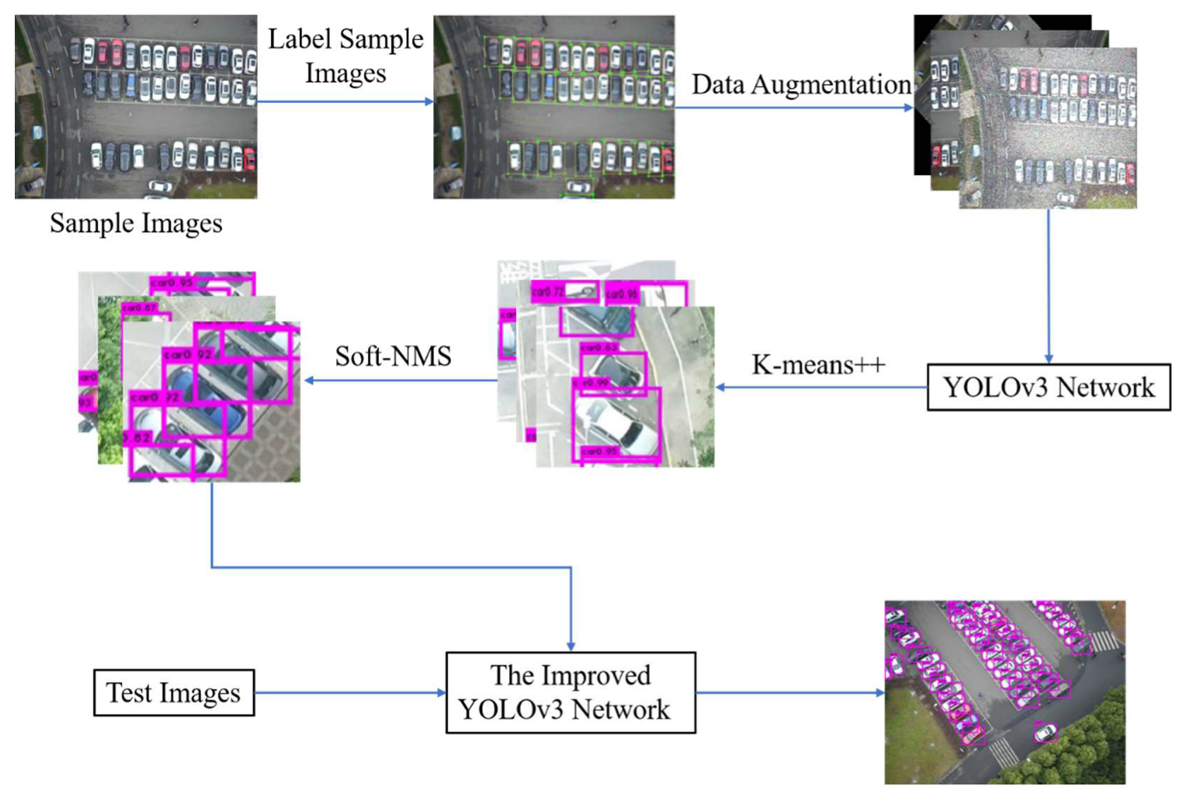Figure 1 demonstrates our proposed vehicle detection framework based on the YOLOv3 network.

2.1. YOLOv3 for Vehicle Detection

The main calculation process of YOLOv3 is indicated below. Firstly, feature extraction is performed on the input to obtain a feature map of a certain size, such as 13 × 13 (169), then the network divides the input image into 169 grid cells of a uniform size. If the center point’s coordinates of an object’s ground truth in the image falls in a grid cell, then the grid cell is responsible for predicting the object. Each grid cell in the image will generate a fixed number of prediction boxes. YOLOv3 combines the features of the first two layers to make predictions together, and create nine prediction boxes in total. The scale of the prediction box of each grid cell is different. The selection of the prediction box is determined by the intersection over union (IOU) of each prediction box and the prediction box actually marked. The one with the largest IOU will be chosen as the target prediction box. The 75th to 105th layers of the feature extraction network are the feature interaction layers of the YOLO network, which are divided into three parts. In each part, convolutional kernels are used to implement local feature interaction. The function of this process is similar to the fully connected layer of the network (the fully connected layer of the network applies global feature interaction), but it realizes a local feature interaction between feature map points based on convolution kernels (1 × 1 and 3 × 3).

When training the YOLOv3 network, the loss function is specified as follow:

$$\begin{array}{l}Loss=\frac{1}{2}{\displaystyle \sum _{i=1}^{10647}}{\lambda }_{\mathrm{obj}}\times [(2-{\mathrm{truth}}_w\times {\mathrm{truth}}_h)\times {\displaystyle \sum _{r\in (x,y,w,h)}{({\mathrm{truth}}_r-{\mathrm{predict}}_r)}^2}+\\ +{\displaystyle \sum _{r=0}^{k-1}{((r=={\mathrm{truth}}_{\mathrm{class}})?1:0-{\mathrm{predict}}_{{\mathrm{class}}_r})}^2}]\\ \hspace{1em}+{({\mathrm{truth}}_{\mathrm{conf}}-{\mathrm{predict}}_{\mathrm{conf}})}^2\end{array}$$

(1)

The author of YOLOv3, Redmon [18], did not directly provide the loss function in the related published papers, and the current relevant literature only provides the loss function of YOLOv1. The loss function listed in this article is summarized in the literature of Lyu [21] based on the source code analysis of Darknet-53 (YOLOv3 network implemented by Redmon). This analytical loss function mainly includes three parts: coordinate loss, confidence loss and classification loss. λ_obj is set to 1 when there is a target object in a grid cell, otherwise it is 0, and it is calculated by SSE (Sum of Squared Error). The final calculated value is the sum of all the loss functions instead of the average of them. The main reason is that the special prediction mechanism of YOLOv3 will lead to a serious imbalance between positive and negative samples in training sets, especially in the part of confidence loss. For example, when each sample image contains only one target, the positive–negative sample ratio in the part of confidence loss part will drop to as low as 1:10,646. If the average loss is still used, the network will not calculate gradient effectively and the loss value will be close to 0, causing the network prediction output to all become zero. Then, the network will lose its predictive capability.

When training the network, the stochastic gradient descent (SGD) [22] was applied to 10,000 iterations. Our own dataset was divided into 7:3. In total, 70% of the data were used to train the model, and the remaining 30% was used to test the precision of the model. In the training process, each mini batch was 64, which means that a matrix of 64 pictures is inputted to the network each time. In the beginning, the network was trained with an initial learning rate of 0.0003, and the uniform stepwise rate decay strategy was chosen. The step length was set to 4000 and 6000 iterations, and the learning rate was attenuated by 0.1 times of the value of the previous step. lr_base is the learning rate set at the beginning and γ is a coefficient. The attenuation function is expressed in Equation (2).

$$lr=l{r}_{\mathrm{base}}\times {\gamma }^{\lfloor \frac{\mathrm{iter}}{\mathrm{stepsize}}\rfloor }$$

(2)

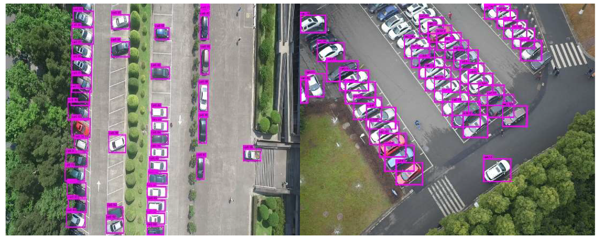
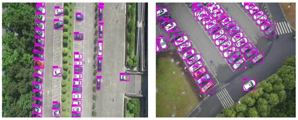
Some test results of YOLOv3 are displayed in Figure 2 below. The batch normalization (BN) layer is added to the YOLOv3 network, which can force the network to converge quickly. Therefore, the value of the loss function tends to be gentle after 1000 iterations. The detailed test results of different training iterations for the test set are provided in

Table 1. Test AP (Average Precision) values of the YOLOv3 network at different training iterations.

Training Iterations	1000	2000	3000	4000	5000	6000	7000	8000	9000	10,000
AP (%)	83.20	86.70	89.10	92.01	91.89	91.88	90.20	90.89	91.52	91.52

. The network reached the optimal solution when the network was trained for 4000 iterations and the test average precision (AP) was 92.01%. After the AP value reached the peak, the network began to over fit, and its detection capability began to decline.

The network with the parameters at 4000 iterations was applied to the test set, and the results are listed in

Table 2. YOLOv3 test results at 4000 iterations.

AP (%)	Recall Rate (%)	Precision (%)	Omission Ratio (%)	Fall-Out Ratio (%)
92.01	94.23	99.74	5.77	0.26

.

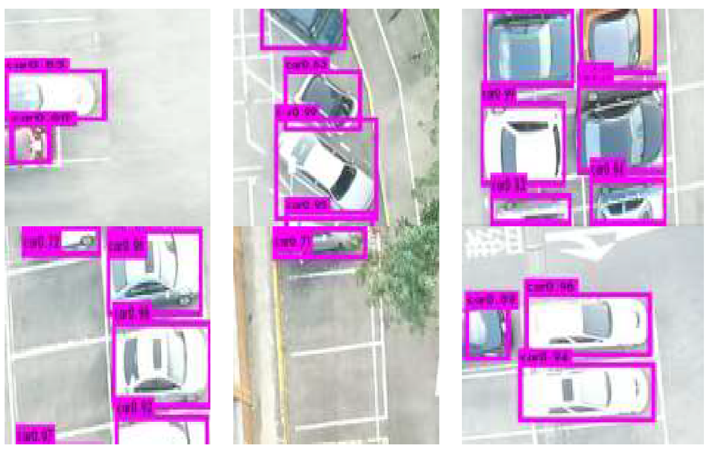
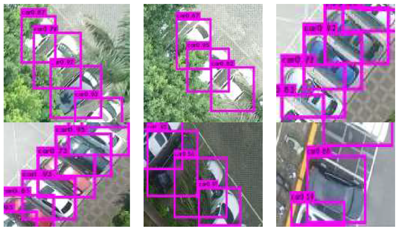
In the test examples, it can be seen that the missed targets of the detection network mainly include two categories. Category one is the partially occluded targets. Most missed targets fell into this category. An example is displayed in Figure 3. The other category is the vehicles whose parking directions are not parallel to UAV images’ margins. Since boxes can only be drawn parallel to the image border when marking targets, the boxes of those targets that are very close and tilted have a high probability of partially overlapping. At the end of the network recognition, there are multiple boxes for each target, with a high degree of overlapping. The original YOLOv3 network utilizes the NMS algorithm to suppress them except the one with the most confidence value. However, if the distance between two targets is short, their boxes also have a high degree of overlapping. When the NMS algorithm is performed, the right boxes are directly suppressed, which leads to a missed detection of the targets. Some omission examples of the wrong multi-box suppression by NMS is given in Figure 4.

2.2. Improvement

In this study, according to the characteristic of vehicles, the detection capability of YOLOv3 can still be enhanced. The original version of YOLOv3 predicts target positions and classification at multiple scales. The initial anchors are derived from the label box clustering. Anchors may be regarded as detection box candidates. The performance of the K-means algorithm used for clustering depends on the selection of the initial value to a large degree. Many images of the large-scale UAV datasets are acquired above parking lots. Generally, the vehicles in parking lots are very close to each other, and especially if their images are acquired from an angle, the marking box overlap between two vehicles is very high. Therefore, the direct usage of NMS is likely to cause the missed detection of some highly overlapping targets. To address the two problems, the K-means++ algorithm and Soft-NMS algorithm were employed.

2.2.1. K-Means++ for Improving Initial Recognition Boxes

In this work, the K-means++ algorithm [19] is used to cluster the label boxes of vehicle targets in the training dataset with K = 9. The purpose of clustering was to enlarge the IOU value of anchors and adjacent ground truth. IOU value is not directly related to the size of the anchor boxes. However, whether distance measurement can be used in the clustering process is a problem worthy of consideration. If the Euclidean distance is employed, it will cause more errors of big anchors than of small ones. Therefore, another distance measurement is used here. The distance formula used for clustering is characterized by:

d(box, centroid) = 1 − IOU (box, centroid)

(3)

Generally, the clustering center of the K-means algorithm needs to be manually specified. The selection of the initial value is an important influence factor of clustering results. The different initial clustering centers may create completely different results. The K-means++ algorithm, as an improved version of the K-means, has a function used for selecting initial clustering centers automatically. This strategy promotes the robustness of the K-means++ algorithm.

When selecting the initial clustering center, the K-means++ algorithm randomly chooses a point in a dataset as the center at first, then traverses all other points in the set to calculate the distance D(x) from the center; finally, it chooses a new point in the set as the next center. The selection method is the point with the largest D(x) has the highest probability of being chosen. The last two steps are repeated until the number of cluster centers meets the requirements. This initial clustering center selection method can ensure that the initial clustering centers are as far away from each other as possible to maximize the classification efficiency.

In the experiment, a smaller distance from the object to the cluster center is expected, but as for the IOU, a larger value is expected. Applying 1-IOU in the formula can ensure that the IOU value increases when the distance decreases, and vice versa. The nine cluster centers derived from clustering are used as the initial anchor position for network training. Compared with the common K-means algorithm, this operation can not only improve networks’ convergence speeds and reduce the risk of divergence, but also improve the precision of networks.

The nine anchors in the YOLOv3 network were assigned to the three prediction scales of YOLOv3. In this paper, the ground truth of the training dataset was clustered using the K-means++ algorithm, and the size of the prediction box obtained was 12 × 18, 14 × 36, 20 × 36, 50 × 62, 70 × 92, 80 × 96, 56 × 97, 72 × 132, and 110 × 226. The newly acquired anchor was used to train the network, and the training strategy was as same as the network initial training strategy. The training results are given in

Table 3. Results after using K-means++ clustering.

AP (%)	Recall (%)	Precision (%)	Omission Ratio (%)	Fall-Out Ratio (%)
96.32	97.70	99.76	0.24	2.30

.

Table 3 implies that the precision and recall rate of the network rose significantly, and the detection performance of partially occluded targets was improved compared with Table 2. By using the K-means++ clustering algorithm, the detection results of partially occluded targets were considerably improved. Some detection examples of partially occluded targets are given in Figure 5.

2.2.2. Soft-NMS for Improving Multi-Box Suppression

Usually, NMS is a necessary component in many target detection networks. First, the NMS algorithm sorts detection boxes according to scores. Then, it chooses a prediction box M with the highest score, and if the IOU of the remaining boxes and M exceed a certain threshold, these remaining ones will be discarded. This process will be repeated periodically in the remaining detection box sets, until this set is empty. Therefore, if a target really exists in a detection box whose IOU with another box reaches a threshold, the target will be discarded. Using the Soft-NMS algorithm, we can suppress the detection box with a score that is not the highest but relatively higher. The IOU values of these boxes and the box of the highest score are all greater than the boxes generated though commonly used maximum suppression thresholds. The method can reduce the problem of the missed detection of dense targets to a certain extent and thus can improve the precision of the model.

When the Soft-NMS algorithm was used to realize the vehicle detection, and the following rules are proposed to update the detection box and confidence score [17]:

$$s_i=\{\begin{array}{cc}{s}_i,& \mathrm{iou}(M,b_i)<N_t\\ s_i(1-\mathrm{iou}(M,b_i)),& \mathrm{iou}(M,b_i)\ge N_t\end{array}$$

(4)

where B = {b₁, …, b_N} is the list of initial detection boxes, S = {s₁, …, s_N} contains the corresponding detection scores, and N_t is the NMS threshold. The above functions (Equation (4)) reduce the scores of the detection boxes whose threshold is above N_t though a linear function of their overlap with M. Those detection boxes far from M are not affected, but those that are very close will be punished more. The above formula is not a continuous function of overlapping degree, and a sudden penalty is added to the threshold when the score reaches N_t. If the penalty function is continuous, its capability may be better; otherwise, it produces a mutation. For these boxes to be suppressed, a continuous penalty function has no penalty for those boxes that do not overlap, and a higher penalty for those boxes that have a high overlap. When the overlap is low, the penalties should be gradually increased because the confidence scores of those detection boxes with a low overlap should not be affected. However, when the overlap degree of the detection box with M is close to 1, the confidence of the detection box should receive a more significant penalty. Considering the above situations, an update to the above penalty function is proposed using a Gaussian penalty function, as depicted in Equation (5) [20]:

$$s_i=s_i{e}^{-\frac{\mathrm{iou}{(M,b_i)}^2}{\sigma }},\forall b_i\notin D$$

(5)

where σ is set to 0.5 and the final threshold is set to 0.001. The updated rules are applied to each iteration, and the confidence scores of all remaining detection boxes will be updated.

With K-means++ clustering in the YOLOv3 network, the Soft-NMS algorithm is used to replace the NMS algorithm. The test results obtained by the improved network at different training iterations are presented in

Table 4. Test AP values of the improved YOLOv3 network at different training iterations.

Training Iterations	1000	2000	3000	4000	5000	6000	7000	8000	9000	10,000
AP (%)	86.25	89.62	93.56	96.38	97.20	97.49	96.55	97.12	93.12	94.51

.

Table 4 presents that the network obtained the best results with 6000 iterations. The test results of the network with 6000 iterations are listed in

Table 5. Results after using Soft-NMS.

AP (%)	Recall (%)	Precision (%)	Omission Ratio (%)	Fall-Out Ratio (%)
97.49	98.74	99.66	0.34	1.26

.

After using the Soft-NMS algorithm, the overall performance of the network was just improved slightly. The reason is that the targets suppressed by the NMS only occupy a small part of the training dataset. With the Soft-NMS, some detection examples in Figure 6 illustrate that the detection capability of partially occluded vehicle targets of the proposed detection framework is enhanced through Soft-NMS multi-box suppression. Some detection examples of the YOLOv3 network are shown in Figure 7 below. Many vehicles in the figure are not detected by the original YOLOv3 network.

3. Results

In this work, we built our own dataset to train and test vehicle detection networks in the experiment. In order to study the generalization performance of the detection network trained by our Class-Car dataset, we used three public datasets for verification. They are CAR, VEDAI, and COWC datasets.

3.1. Data Acquisition and Construction

The UAV vehicle dataset used in this work was constructed independently by our team. In the following, Class-Car will be used to refer to this dataset. According to our statistics, a total of 1978 UAV images were used, including nearly 100,000 vehicle targets.

During the training process, too few training data samples may cause the network to over fit. Therefore, data augmentation technology was used to expand the image data of Class-Car. The methods included: 1. Random rotation. The image was randomly rotated at any angle (0° to 360° degrees); 2. Mirror flip. The image is flipped up and down or left and right; 3. Color dithering. The images’ saturation, brightness, contrast, and sharpness are randomly adjusted; and 4. Gaussian noise is added to images [23].

By augmenting training samples, disturbances to the targets’ color and texture and changes from the rotation and scaling existing in UAV images can be effectively relieved. Though expanding the original dataset with 1978 positive samples five times, 11,868 images with corresponding label files can be generated, of which 30% is randomly chosen as the test set and the remaining images are used for training. The ratio of training and testing was 7:3. Figure 8 describes the results of a random sample in the original dataset, processed after data augmentation.

3.2. Result for Test Images

The real loss function is depicted in Figure 9a and Figure 10a, which indicates that either before or after the network is improved, the network rapidly converges during the first 1000 iterations and the value of the loss function decreases rapidly. After that, the process becomes stable. When visualizing the training results in Figure 9 and Figure 10, we only exhibited the results of the first 800 iterations to avoid the compression of curves and plot the initial iteration process more clearly. The initial value of the loss function of the improved network was larger than of the original network. The reason is that the K-means++ algorithm was used to cluster the training dataset. The obtained anchor initial positions were closer to the dataset than the ones created by the original network, so the initial value of the loss function of the improved network was smaller. Although the network quickly converged in the early stage, after 1000 iterations, the loss function of the network did not change much, but the original network reached the highest precision at 4000 iterations, and the improved network reached the highest precision at 6000 iterations. Hence, the convergence speed of the improved network slightly decreased.

An analysis of the PR curve of networks is also important. Figure 9b draws the PR curve for the test dataset after the original YOLOv3 model learned the dataset. Figure 10b illustrates the PR curve for the test dataset after the improved YOLOv3 learning the dataset, and the resulting model’s PR curve. From the PR curve, before and after the improvement, when the value of recall is relatively low, the overall performance difference is not obvious. But when the value of the recall rate rises to 0.8, the overall performance the improved YOLOv3 is better than the original one. An analysis of

Table 6. Comparison of the test indicators.

Method	AP (%)	Recall Rate (%)	Precision (%)	Omission Ratio (%)	Fall-Out Ratio (%)
YOLOv3	92.01	94.23	99.74	5.77	0.26
YOLOv3 with K-means++	96.32	97.70	99.76	0.24	2.30
YOLOv3 with K-means++ and Soft-NMS	97.49	98.74	99.66	1.26	0.34
Faster R-CNN	80.50	81.70	89.40	17.30	10.60
Improved Faster R-CNN	90.60	90.70	96.40	9.30	3.60

suggests that the network lost a small amount of precision (from 99.74% to 99.66%, a decrease of 0.08%) in exchange for a large growth in the recall rate (from 94.23% to 98.74%, an increase of 4.51%) and AP (from 92.01% to 97.49%, an increase of 5.48%). The improvement strategy considerably enhanced the overall performance of the entire network. The K-Means++ algorithm contributed 4.31% to the AP value of the network, while the Soft-NMS algorithm improved the AP value by 1.17%.

After the K-Means++ algorithm was used to improve the YOLOv3 network, we tested the network using the Class-Car dataset. The detection capability of the network on partially occluded targets significantly improved (the omission ratio dropped from 5.77% to 0.24%), but the fall-out ratio increased (from 0.26% to 2.30%). After the application of Soft-NMS, the detection capability of the network for dense targets rose, and the fall-out ratio returned to a lower level (0.34%), while the omission ratio increased to a certain extent (up to 1.26%), and still remained at a low level. For comparison, we also tested the Faster R-CNN and our improved version [24] with the Class-Car dataset. Table 6 also proves that the indicators of the improved YOLOv3 network are superior to both Faster R-CNN and our improved Faster R-CNN.

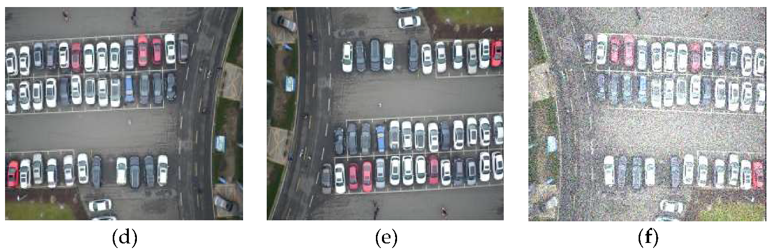
3.3. Result for COWC

The Cars Overhead with Context (COWC) dataset is widely used for deep neural network training. The images in this dataset are acquired from mid-distance and overhead point view. The image resolution is 15 cm per pixel, and the data contain 32,716 marked vehicles and 58,247 negative samples. The data were collected from six different locations: Toronto, Canada; Selwyn, New Zealand; Potsdam and Vaihingen, Germany; and Columbus, Ohio, and Utah, USA. The original COWC images are relatively large, and sample images in COWC were made by cropping large ones. Each scene of original images occupies a large urban area, which results in fewer pixels being occupied by vehicle targets in sample images, the image being more blurred, and features being difficult to extract, making recognition difficult. In our test, original images were enlarged, then some local regions in the whole image were captured, and finally it was put into the network for testing.

Table 7. Verification results for COWC.

Method	AP (%)	Recall Rate (%)	Precision (%)	Omission Ratio (%)	Fall-Out Ratio (%)
YOLOv3	65.9	82.2	75.1	17.8	24.9
Improved YOLOv3	69.1	83.8	77.9	16.2	22.1

presents the verification results of the improved YOLOv3 for COWC. Figure 11 displays some detection examples. Table 7 indicates that the two trained networks can detect vehicle targets in strange dataset, and the improved YOLOv3 network outperformed the original one.

3.4. Result for VEDAI

Vehicle Detection in Aerial Imagery (VEDAI) is an efficient tool to examine automatic target recognition algorithms in unconstrained environments. It is derived from satellite images. The vehicles contained in this database, are too small and exhibit different variation, such as multiple orientations, lighting/shadowing changes, specularities, or occlusions [25].

Table 8. Verification results for VEDAI.

Method	AP (%)	Recall Rate (%)	Precision (%)	Omission Ratio (%)	Fall-Out Ratio (%)
YOLOv3	60.2	77.2	72.6	22.8	27.4
Improved YOLOv3	71.2	80.7	83.5	19.3	16.5

and Figure 12 give the verification results for VEDAI and some detection examples of the improved YOLOv3. Although it was found that the performances of the two networks deteriorated significantly, the detection capability of the improved YOLOv3 is more acceptable than the original network.

3.5. Results for the CAR Dataset

The Chinese Academy of Sciences CAR dataset is taken from Google Earth, containing both satellite and airborne images. From the verification results presented in Figure 13 below, the recognition capability of the networks for blurred images was found to be still relatively effective, but the test results for the images of different point views were not very satisfactory. The primary reason of this was the apparent difference between the verification image and the network training sample, and the second reason was the lack of diversity in the training images.

Table 7, Table 8 and

Table 9. Verification results for CAR.

Method	AP (%)	Recall Rate (%)	Precision (%)	Omission Ratio (%)	Fall-Out Ratio (%)
YOLOv3	64.4	72.8	78.4	27.2	21.6
Improved YOLOv3	68.5	76.5	79.6	23.5	20.4

describe that with the appropriate improvements, the YOLOv3 network enhanced the recognition precision of vehicle targets on different datasets to different degrees, which proves the effectiveness of our proposed detection framework. The three vehicle image datasets chosen for generalization performance verification are quite different from our Class-Car dataset in terms of the resolution, shooting angle, and shooting area of the images, as well as the sizes of vehicle targets, which considerably and objectively reduced the precision of detection.

4. Conclusions

In this paper, to solve the problem of vehicle detection in UAV images, a deep-learning-based convolutional neural network, the YOLOv3 algorithm, was utilized to achieve accurate vehicle detection and localization. A large-scale vehicle target recognition dataset, based on UAV images, was built, including a total of 1978 pictures and nearly 100,000 vehicle targets. The YOLOv3 network was applied to the target recognition task in the UAV images, and it was improved based on the characteristics of vehicles. On the basis of YOLOv3, the K-means++ algorithm was employed to improve the selection of the initial recognition box, which enhanced the AP value of the network by 4.31%. Then, Soft-NMS was applied to relieve the problem of the wrong of multi-box suppression by NMS, which enhanced the AP of the network by 1.17%. The AP value of the entire network was improved by 5.48% totally, and the omission ratio of the entire network was decreased by 4.51%.

We chose three public datasets with different image quality to verify the generalization of the improved networks. From the experimental results, it is found that the improved YOLOv3 algorithm possesses high precision and fast recognition speed. The experiment proved that our detection framework has a strong capability and good adaptability.

Since our improvement is based on the characteristics of vehicle targets, we think that targets with similar characteristics can also be detected by our proposed method. In this work, the detection object was specified by a small size and dense distribution. Our proposed framework can also be modified in other means (for example, serving as a pre-training model in transfer learning, etc.) to identify other targets, such as passenger cars, ambulances, tanks, aircrafts, and ships. These research works are in progress.