Article

A Comparison of Three Trapezoid Models Using Optical and Thermal Satellite Imagery for Water Table Depth Monitoring in Estonian Bogs

1
Institute of Ecology & Earth Sciences, Department of Geography, University of Tartu, 46 Vanemuise St., 51014 Tartu, Estonia
2
Department of Earth and Environmental Sciences, KU Leuven, 3001 Heverlee, Belgium
3
Department of Computer Science, KU Leuven, 3001 Heverlee, Belgium
4
Chair of Data Science, Institute of Computer Science, University of Tartu, 2 J. Liivi St., 50409 Tartu, Estonia
*
Author to whom correspondence should be addressed.
Remote Sens. 2020, 12(12), 1980; https://doi.org/10.3390/rs12121980
Submission received: 6 May 2020 / Revised: 8 June 2020 / Accepted: 17 June 2020 / Published: 19 June 2020
(This article belongs to the Special Issue Remote Sensing of Wetlands)

Abstract

:
This study explored the potential of optical and thermal satellite imagery to monitor temporal and spatial changes in the position of the water table depth (WTD) in the peat layer of northern bogs. We evaluated three different trapezoid models that are proposed in the literature for soil moisture monitoring in regions with mineral soils. Due to the tight capillary connection between water table and surface soil moisture, we hypothesized that the soil moisture indices retrieved from these models would be correlated with WTD measured in situ. Two trapezoid models were based on optical and thermal imagery, also known as Thermal-Optical TRApezoid Models (TOTRAM), and one was based on optical imagery alone, also known as the OPtical TRApezoid Model (OPTRAM). The models were applied to Landsat imagery from 2008 to 2019 and the derived soil moisture indices were compared with in-situ WTD from eight locations in two Estonian bogs. Our results show that only the OPTRAM index was significantly (p-value < 0.05) correlated in time with WTD (average Pearson correlation coefficient of 0.41 and 0.37, for original and anomaly time series, respectively), while the two tested TOTRAM indices were not. The highest temporal correlation coefficients (up to 0.8) were observed for OPTRAM over treeless parts of the bogs. An assessment of the spatial correlation between soil moisture indices and WTD indicated that all three models did not capture the spatial variation in water table depth. Instead, the spatial patterns of the indices were primarily attributable to vegetation patterns.

Graphical Abstract

1. Introduction

Knowledge of soil moisture is important for a wide range of applications in hydrology, meteorology, climatology, and biogeochemistry [1,2,3]. Soil moisture is pivotal to understand dynamics of net ecosystem exchange and ecosystem feedbacks to global climate change [4]. This is especially the case for peatlands that are defined by a surface soil layer of peat that is at least 30 cm thick and that act as large terrestrial carbon pools [5,6,7]. The soil moisture in surface peat layers and the position of the water table in the peat layer relative to the ground surface, i.e., the water table depth (WTD), are important features of peatlands, as they control the interface between aerobic and anaerobic conditions. This, in turn, causes a shift in fluxes of CO2, N2O, and CH4 [8,9,10].
Mineral and peat soils differ from each other primarily in the proportion of solid inorganic and organic particles, leading to differences in their hydraulic properties [11,12]. Within a region with mineral soils, the spatial differences in water retention curves can be attributed to a mineral texture (from sand to clay) [13,14], while, in peat soils, differences can be attributed to the vegetation and the related plant debris, and its degree of decomposition over time [15]. The temporary unsaturated surface layer of the peat profile (acrotelm) is characterized by a high organic matter content that is poorly decomposed. This structure of the acrotelm leads to a high water storage capacity and high hydraulic conductivity [16,17,18].
Shallow WTD conditions and the typical hydraulic properties of the acrotelm cause a tight connection between WTD and soil moisture content in peatlands [7,19,20,21,22,23,24]. In several studies, the tight connection is illustrated by scatter plots of temporal data of soil moisture and WTD at individual locations. In these plots, points typically align in narrow bands, which indicates that a new soil water equilibrium is quickly established after a precipitation event. Figure 1 illustrates how this tight connection can be used to derive information about WTD dynamics in time from the surface characteristics sensed with optical and thermal satellite imagery. Note that the soil moisture in peatlands is highly variable at the scale of a few meters due to the presence of small-scale elevation differences also known as hummock and hollow microtopography. The typical optical and thermal satellite imagery has a spatial resolution of tens of meters and integrates over this small-scale variability.
Different types of satellite observations have been used to estimate soil moisture. The large difference between the dielectric constants of water (~80) and soil particles (~4) permits the monitoring of soil moisture with passive and active microwave remote sensing [25,26,27,28]. Microwave observations have the advantage that they are directly sensitive to soil moisture, although the sensing depth is typically limited to the top few centimeters of soils. The longer wavelength (L band) of the passive microwave satellite missions that are currently dedicated to soil moisture monitoring are less sensitive to vegetation than the operational active microwave missions. However, the passive observations have a coarse resolution (~40 km) [25,26], whereas some active missions allow high spatial resolution mapping (<100 m) [29,30]. A few studies have analyzed and used passive [31,32,33] and active [34,35] microwave measurements for the purpose of soil moisture monitoring in peatlands. One of the major constraints of applicability of active microwave observations over peatlands is a dependency of radar signal on land surface properties [36]. The microwave backscatter signal over natural peatlands showed a low sensitivity to WTD dynamics, which might be related to strong confounding effects that occur due to complex scattering in vegetation and the fibric surface peat layer [37,38,39,40].
Soil moisture can also be estimated using optical and thermal imagery. One of the most well-known approaches for soil moisture estimation is the “trapezoid”, or “triangle”, model concept [41,42]. The concept takes advantage of the existence of a relationship between optical and thermal land surface properties and soil moisture [43,44]. Due to the high sensitivity to vegetation properties, such as the moisture status in the plants, it is proposed that derived moisture estimates also reflect the root-zone moisture [44].
Two different types of the trapezoid concept exist and they mainly differ in the used moisture-sensitive signal. One of the types uses the land surface temperature (LST) and the physical principle of evaporative cooling (wetter = cooler); the other one uses the strong absorption of shortwave infrared (SWIR) radiation of water and calculates the shortwave infrared transformed reflectance (STR) from SWIR [44]. In both types, the moisture-sensitive signal is combined with a vegetation index (VI), e.g., the normalized difference vegetation index (NDVI) or the fractional vegetation cover (FVC), to construct a trapezoid space [44,45,46,47,48,49,50]. The lowest LST or highest STR along the vegetation cover gradient defines the wettest soil moisture, whereas the highest LST or lowest STR defines the driest soil moisture in the landscape. The trapezoid space is then used to linearly scale soil moisture. The type of trapezoid model that utilizes LST is further called the Thermal-Optical TRApezoid Model (TOTRAM) [42,51,52,53,54], and the type of trapezoid model that utilizes STR is further called the OPtical TRApezoid Model (OPTRAM) [44].
There exist several different algorithms of the TOTRAM concept. One type of algorithm derives the dry edge directly from the LST over the driest areas in the scene. In another type of algorithms, additional weather data are used to theoretically estimate the temperature of the driest land fraction, which then defines the dry edge of the trapezoid space [55,56].
Previous studies evaluated the applicability of TOTRAM and OPTRAM mainly in mineral soils [44,48,57,58,59]. Very little attention has been paid to the models’ applicability in organic soils [60,61]. In this study, we explored the feasibility of applying the TOTRAM and OPTRAM soil moisture indices for the WTD monitoring in two ombrotrophic peatlands, i.e., bogs, in Estonia. The specific objectives of this study were: (i) to estimate the soil moisture indices based on two different TOTRAM and one OPTRAM concepts proposed in the literature, using Landsat 5, 7, and 8 observations for the growing seasons of 2008–2019; and (ii) to evaluate the temporal and spatial correlation of the indices with in-situ measured WTD of the same period.

2. Materials and Methods

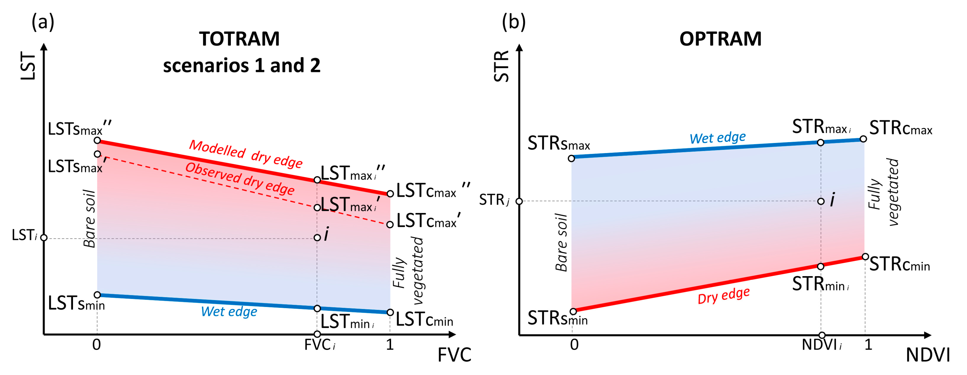
2.1. Trapezoid Models

2.1.1. TOTRAM: Thermal-Optical Trapezoid Model

TOTRAM is one of the most widely used approaches to estimate surface moisture from remote sensing data over mineral soils [42,53,54,62,63]. Initially, this method was developed to interpret the trapezoidal-shaped distribution of pixel values in the space defined by LST and a vegetation index (VI), such as FVC, NDVI, or leaf area index (LAI) [47,48,64]. The highest and lowest values of LST along the vegetation cover gradient represent the so-called dry and wet edges (Figure 2). The wet and dry edges are isopleths and indicate the uniform soil moisture availability for two extreme surfaces: wet and dry [42,46]. Evapotranspiration on the wet edge is maximum and not limited by water availability, whereas evapotranspiration at the dry edge is minimum because of extreme water limitation [42]. In addition to the wet and dry edges, more isopleths could be drawn indicating transitional moisture condition [65]. Consequently, the TOTRAM soil moisture index, WTOTRAM, of each pixel i is calculated on the basis of its position relative to the wet and dry edges within LST-VI space at a single time step or scene,
W T O T R A M , i = L S T m a x , i L S T i L S T m a x , i L S T m i n , i
where LSTi is the LST value of the pixel i and LSTmax,i and LSTmin,i are the LST values of the dry and wet edge at FVCi (Figure 2a).
The accuracy of the TOTRAM depends on several criteria:
  • Negligible spatial variability in weather conditions. The study area should be limited and have a minimal topographic variation to guarantee that the location of the isopleths within LST-VI space is determined by the water availability and not by the difference in atmospheric conditions. For this reason, TOTRAM also demands an individual parameterization of the trapezoid space for each observation scene.
  • Negative temporal correlation between LST and VI at a given location. The temporal applicability of the TOTRAM concept requires that LST decreases not only in space but also in time with increasing VI [66,67].
We applied two different TOTRAM scenarios from the literature that differ in the treatment of these application criteria in the context of the dry edge determination.

Scenario 1: Observed Dry Edge

In Scenario 1, the trapezoid was solely based on observed pixel values. This scenario requires a sufficient range in vegetation and moisture conditions. The study area should be large enough to include sufficient land surface variability for a precise determination of the dry and wet edges [46]. The area size needs be balanced against the TOTRAM requirement of homogenous weather conditions. The dry and wet edges were determined from the observed highest and lowest LST values along the FVC gradient following the algorithm in [41]. This algorithm splits the LST pixels based on FVC values in LST–FVC space into 20 intervals and, after that, each interval into 5 subintervals. For each interval, the minimum and maximum LST values are calculated. Thereafter, the wet and dry edges are modeled as the linear fit to the mentioned minimum and maximum LST values.

Scenario 2: Modeled Dry Edge

During wet periods following widespread precipitation, the dry edge is difficult to define based on observed pixel values alone. To cope with this limitation, it has been proposed to derive the dry edge theoretically, i.e., based on models [55,68,69]. In Scenario 2, the modeled dry edge was determined by two modeled temperatures: the temperature of the driest bare surface (LSTsmax) and the driest fully vegetated surface (LSTcmax) (Figure 2a). Because the in-situ meteorological measurements needed for modeling the dry edge were only available starting from June 2009, Scenario 2 was applied for a shorter period (2009–2019). We followed the algorithm for retrieving LSTsmax and LSTcmax developed by Long et al. [55], which is based on solving for the system of physically-based non-linear equations in an iterative manner (Appendix A and Appendix B). Knowing these two extreme temperatures, it becomes possible to model the theoretical dry edge with linear regression approach, where (LSTcmax-LSTsmax) is a slope and LSTsmax is an intercept.

2.1.2. OPTRAM: Optical Trapezoid Model

Sadeghi et al. [44] introduced the concept of OPTRAM which uses STR as soil moisture sensitive parameter. Figure 2b illustrates the concept of OPTRAM. In OPTRAM, the trapezoid is formed by NDVI as a measure of vegetation cover and STR as a measure of moisture content [70,71,72]. In contrast to LST, STR is not assumed to depend on the specific weather conditions, and the trapezoid can therefore be determined based on observations across all observed scenes. To determine the wet and dry edges, firstly, we randomly sampled 10% (approximately four million in space and time) of the pixels from the total dataset. Secondly, the full range of sampled NDVI values was divided into 100 intervals. Within each interval, the median, standard deviation, maximum, and minimum STR values were obtained. The dry edge was distinct and clearly observable, and it was modeled as a linear fit to the minimum STR values. Due to several obvious outliers caused by open water surfaces and remaining shadow effects, the wet edge was less explicitly defined than the dry one and it was modeled as a linear fit to the “median + standard deviation” values of the 100 intervals.
As noticed by Sadeghi et al. [44], OPTRAM approach is sensitive to oversaturated pixels. Therefore, we excluded pixels with negative NDVI values which correspond to water, as suggested by Babaeian et al. [58]. Additionally, all the pixels located above the wet edge were excluded from further statistical analysis.
The OPTRAM soil moisture index, WOPTRAM, is then derived by a linear scaling between the maximum and minimum STR for a specific value of NDVI,
W O P T R A M , i = S T R i S T R m i n , i S T R m a x , i S T R m i n , i
where STRi is the STR value of the pixel i, while the STRmax,i and STRmin,i are the STR values of the dry and wet edge at the NDVI of pixel i (Figure 2b).

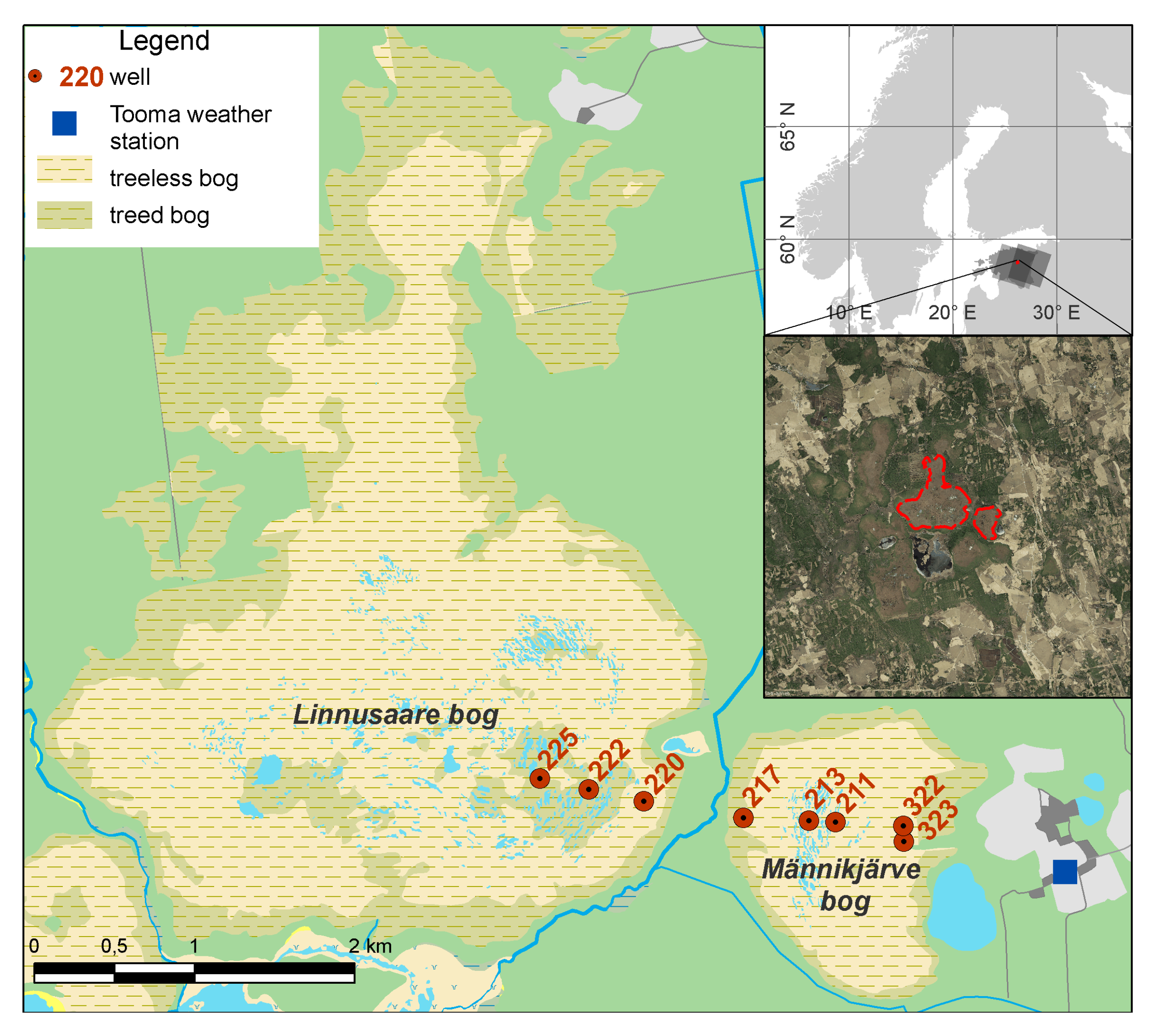
2.2. Study Area and Field Measurements

Our study focused on the two bogs, Linnusaare and Männikjärve, because of their available long-term records of WTD, which were measured since 1950 [73,74,75]. These bogs belong to the Endla mire system and they are located in eastern central Estonia (Figure 3). The climate of the study region is temperate transitional between maritime and continental. The annual precipitation is about 660 mm and the average annual temperature is 5.2 °C. The bogs are of limnogenic origin and located within the East-Baltic Bog Province [76]. The tree layer of both bogs consists mainly of sparse Scots pines (Pinus sylvestris). In the inner-bog area, dwarf pines grow on ridges and they mark the treed ridge-hollow and treed ridge-pool complexes. The pine forest grows only at the bog’s edges. The grass and dwarf shrub layers consist of Calluna vulgaris, Eriophorum vaginatum, Chamaedaphne calyculata, Andromeda polifolia, Rhynchospora alba, Ledum palustre, Oxycoccus microcarpus, and Oxycoccus palustris [77]. The typical moss species are Sphagnum fuscum, Sphagnum balticum, Sphagnum magellanicum, and Sphagnum rubellum [77]. Nowadays, Linnusaare and Männikjärve bogs have a conservation status and are on the list of Ramsar Sites [78].
Air temperature and air pressure were measured at hourly resolution at Tooma weather station beginning from June 2009 (Figure 3) [80]. Eight WTD monitoring wells were installed in hollows along a transect (Figure 3). All the WTD measurements were referenced to the average height of the hollow surface. WTD was measured in sampling wells of 150 cm depth and 20 cm diameter; wells were permeable for water over the full length. In this study, we used daily measured WTD data from the growing seasons (May to September) from 2008 to 2019. The temporal dynamics in WTD were similar in different parts of the bogs. We observed a strong temporal correlation between WTD data from eight wells (Pearson correlation coefficients vary from 0.85 to 0.96). In addition, over short distances of a few meters, previous studies have shown only very small hydraulic gradients between hummock and hollow locations that can be neglected for our type of study [81]. However, the amplitudes of WTD fluctuation did differ: fluctuations were lower for the central part and higher for the bog edges, which is a peculiarity of peatland hydrology [82].

2.3. ERA 5 Data

ERA 5 is the atmospheric reanalysis of the global climate produced by the European Centre for Medium-Range Weather Forecasts [83]. ERA5 provides hourly atmospheric parameters as regular latitude-longitude grids at 0.25° spatial resolution. Data of friction velocity and total column water vapor were used to perform the modeling of the dry edge required for TOTRAM Scenario 2 (Appendix A and Appendix B). We selected ERA 5 data which in terms of the time were the nearest to Landsat acquisition time.

2.4. Remote Sensing Sources and Ancillary Data

Remotely sensed Landsat and MODerate-resolution Imaging Spectroradiometer (MODIS) images together with National Centers for Environmental Prediction and the National Center for Atmospheric Research (NCEP/NCAR) reanalysis data were used for the growing seasons from 2008 to 2019. Data processing was performed on the Google Earth Engine (GEE) online platform.
We processed Landsat 5 data for the time period between 2008 and 2012 since Landsat 5 was decommissioned in 2013. The resolution of visible and near-infrared (VNIR) bands is 30 m. Additionally, Landsat 5 had one thermal infrared band originally sensed with a resolution of 120 m and later resampled to 30 m. Landsat 7 data, unlike Landsat 5 and 8 data, cover the entire period of our study. Its data are recorded in 8 spectral bands; VNIR data have a spatial resolution of 30 m, but thermal data are recorded with 60 m spatial resolution and later resampled to 30 m [84]. Due to the Landsat 7 Scan Line Corrector failure, the study area was partly covered with stripes of missing data. We did not apply any blending techniques to fill in stripes of missing data. Landsat 8 (launched in 2013) data cover only the last six years of our study period. It provides data with the same spatial resolution as Landsat 7, except for the two thermal bands, which are recorded with 100 m spatial resolution and resampled to 30 m [85].
Each Landsat satellite overflew the study area every 8 days since the study area overlaps with two Landsat paths: 186 and 187 (Figure 3). For the next processing steps, we used only those Landsat images that included at least 400 of the 10,549 bog pixels after filtering the pixels affected by shadows, clouds, and Landsat 7 scan-line-off stripes. This minimum threshold was subjectively defined to include a sufficient amount of bog pixels during the definition of the trapezoid space. In total, 168 Landsat images were selected for further calculation and analysis. We used the following Landsat products: at-sensor radiance, brightness temperature, cloud mask, and metadata information about solar zenith angle and relative Earth–Sun distance.
MODIS aboard Terra provides MOD11A1 V6 product, which includes LST and emissivity data. Both have 1 km spatial resolution and were daily sensed over the study area. We used the MODIS emissivity product sensed in two bands, namely 31 and 32, which in terms of acquisition time was the nearest to the Landsat acquisition time.
The data of atmospheric water vapor content produced by NCEP/NCAR were used. This dataset is available in GEE at 2.5° spatial and six hourly temporal resolutions (00:00, 06:00, 12:00, and 18:00 UTC).

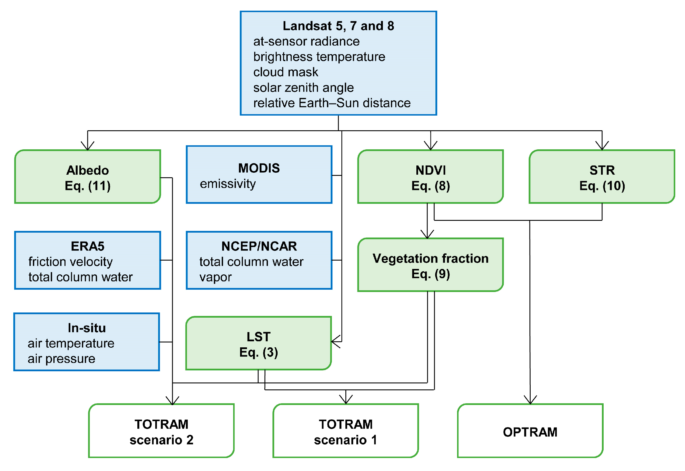
2.5. Variable Derivation

The basic concept of data preparation to derive moisture indices using either of the two TOTRAM scenarios or OPTRAM is presented in Figure 4. The figure illustrates the sequence of data analysis steps with inputs, intermediate variables, and outputs. As mentioned above, in Scenario 1, the TOTRAM estimation was solely based on observed pixel values. The remotely sensed LST and FVC data were used to construct trapezoid and indicate the dry and wet edges. In Scenario 2, in addition to LST and FVC, auxiliary data were used to model LSTsmax and LSTcmax, including friction velocity and total column water vapor data from ERA5, land surface albedo, and in-situ meteorological data. The OPTRAM soil moisture index was calculated based on remotely sensed STR and NDVI data.

2.5.1. Land Surface Temperature (LST)

The single-channel algorithm was used to calculate Land Surface Temperature (LST) for Landsat 5, 7, and 8 data [86]. We implemented the single-channel methodology and calculated LST in GEE following the algorithm described in [87].
The single-channel algorithm requires only one thermal channel to retrieve LST (K),
L S T = γ [ 1 ε ( ψ 1 L s e n + ψ 2 ) + ψ 3 ] + δ
where ε is the land surface emissivity; ψ1, ψ2, and ψ3 are atmospheric functions which can be obtained as a function of the total atmospheric water vapor content w; Lsen is a thermal radiance at sensor level in W m−2 sr−1 μm−1; and γ and δ are two parameters which are dependent on the Planck’s function and were calculated using:
γ T s e n 2 b γ L s e n
δ T s e n T s e n 2 b γ
where Tsen is at-sensor brightness temperature (K) and bγ is 1277 K for Landsat 5 and 7 and 1324 K for the 10th band of Landsat 8.
In Equation (3), the emissivity ε was considered as the average value of bands 31 and 32 provided by MODIS MOD11A1 V6 product. We chose MODIS derived emissivity since it has several advantages for our study. Firstly, the MODIS dataset fully covers the study period. To be precise, GEE provides MOD11A1 dataset available started from 2000 until the present time. Secondly, the algorithm for MODIS emissivity calculation considers the land cover types [88]. The sixth collection of MODIS emissivity product, which is used in this study, includes “Permanent wetlands” as a class of land cover, which likely increases the accuracy of the subsequent LST estimates. Thirdly, previous study has demonstrated the high accuracy of MODIS derived emissivity for LST calculation [87].
GEE gives access to the Landsat products of different processing levels. The dataset with raw scenes contain orthorectified, scaled, and calibrated at-sensor radiance images. The thermal infrared radiance-at-sensor band Lsen was taken from this collection. Another Landsat dataset is the surface reflectance, which is an atmospherically corrected and orthorectified collection of images. This product includes a brightness temperature band Tsen, which was used in LST calculation. In addition, Landsat surface reflectance dataset contains cloud, shadow, and water mask called CFMASK, which we applied for per-pixel quality estimation.
To eliminate the atmospheric effect on LST, Equation (3) includes atmospheric functions (ψ1(w), ψ2(w), and ψ3(w)) and, thus, indirectly accounts for different atmospheric water vapor content (w) across the study time. For atmospheric water vapor content, we used reanalysis data produced by NCEP/NCAR. To cope with time misalignment between Landsat and NCEP/NCAR datasets, we followed the approach presented in [87] and took the value of column water content as the averaged one between two water content values, which were the closest in time to Landsat acquisition time. To calculate atmospheric function for Landsat 5 and 7 we used the following coefficients obtained in [86]:
[ ψ 1 ψ 2 ψ 3 ] = [ 0.14714 0.15583 1.1234 1.1836 0.37607 0.52894 0.04554 1.8719 0.39071 ] [ w 2 w 1 ]
Another matrix of coefficients was used for the 10th band (10.9 μm) of Landsat 8 [89]:
[ ψ 1 ψ 2 ψ 3 ] = [ 0.04019 0.02916 1.01523 0.38333 1.50294 0.20324 0.00918 1.36072 0.27514 ] [ w 2 w 1 ]
Figure 5 shows the time series of LST along with other variables and indices over the studied bog area. For the whole study period, LST values were higher than the air temperature, which is in agreement with the previous study of this bog [80]. LST and air temperature follow similar seasonal curves with maximum values in July.

2.5.2. Normalized Difference Vegetation Index (NDVI)

NDVI was proposed in the 1970s and since that time it has been widely used as an indicator of vegetation photosynthetic activity [90]. NDVI is calculated using near-infrared (NIR) and red reflectivity, ρNIR and ρRed, since chlorophyll in canopy highly reflects in the NIR range and absorbs red wavelengths,
N D V I = ρ N I R ρ R e d ρ N I R + ρ R e d
Figure 5 shows time series of NDVI derived from the Landsat surface reflectance dataset in GEE. CFMASK was used for cloud and shadow masking. The spatial median of the NDVI values varied in time from 0.46 to 0.71. The highest NDVI values were observed in July and August.

2.5.3. Fractional Vegetation Cover (FVC)

FVC was obtained from NDVI through the equation [68,91],
F V C = N D V I N D V I m i n N D V I m a x N D V I m i n
where NDVImax and NDVImin are the maximum and minimum values of NDVI corresponding to the values of dense vegetation and bare soil.

2.5.4. Shortwave Infrared Transformed Reflectance (STR)

STR is a remotely sensed variable used to estimate soil water content [72]. The STR is calculated from SWIR reflectance ρSWIR,
S T R = ( 1 ρ S W I R ) 2 2 ρ S W I R
STR was calculated using the SWIR channel (2210 μm) taken from Landsat surface reflectance dataset. Similar to NDVI, we used CFMASK to mask clouds and shadows. The spatial median of the STR values varied in time between 2.93 and 7.77 (Figure 5).

2.5.5. Broadband Albedo of Vegetated and Bare Surfaces

The broadband albedo was calculated for Landsat data according to the technique proposed by Liang [92],
α = 0.356 ρ B l u e + 0.130 ρ R e d + 0.373 ρ N I R + 0.085 ρ S W I R 1 + 0.072 ρ S W I R 2
where α is a broadband albedo and ρ is surface reflectance measured in blue, red, NIR, and two SWIR spectra. This conversion from narrow- to broadband albedo was originally developed for Landsat 5 and 7, but it is commonly applied also to Landsat 8 bands [93,94,95]. The calculated albedo for a pixel is assumed to be the weighted sum of two components: albedo of canopy αc and albedo of soil αs [55]. To estimate both albedo components, Long et al. [55] suggested fitting a linear model to the maximum α values which lie within the interval “mean plus standard deviation” along FVC axis. This approach is reasonable when a linear relationship is observed between α and FVC. However, many studies revealed a non-linear relationship between α and vegetation cover [96,97,98,99]. We observed in the data of our study area a non-linear relationship between α and FVC and, therefore, the method suggested in [55] was modified. We fitted two linear models: the first one for albedo data with FVC range between 0 and 0.5 and the second one for albedo data with FVC between 0.8 and 1. In such a way, the first model was fitted to the pixels with dominant bare soil, the second one with dense healthy vegetation. Knowing the slope and intercept of the linear model, it became possible to estimate α for dry bare and vegetated surfaces using LSTsmax and LSTcmax (dry edge values, see Figure 2a), considering that their FVC values are 1 and 0.

2.6. Correlation Analysis

We determined the temporal Pearson correlation coefficients (R) between soil moisture indices of the three different trapezoid models and in situ WTD measurements. Anomaly Pearson correlation coefficients (anomR) were calculated to evaluate the capability of the trapezoid models to monitor the short-term and interannual variability of WTD. Anomaly time series of in-situ and soil moisture indices were obtained by removing the multi-year one-month-smoothed average from the original time series values. A limited spatial analysis on the correspondence between in situ WTD patterns and retrieved soil moisture indices was also included.

3. Results

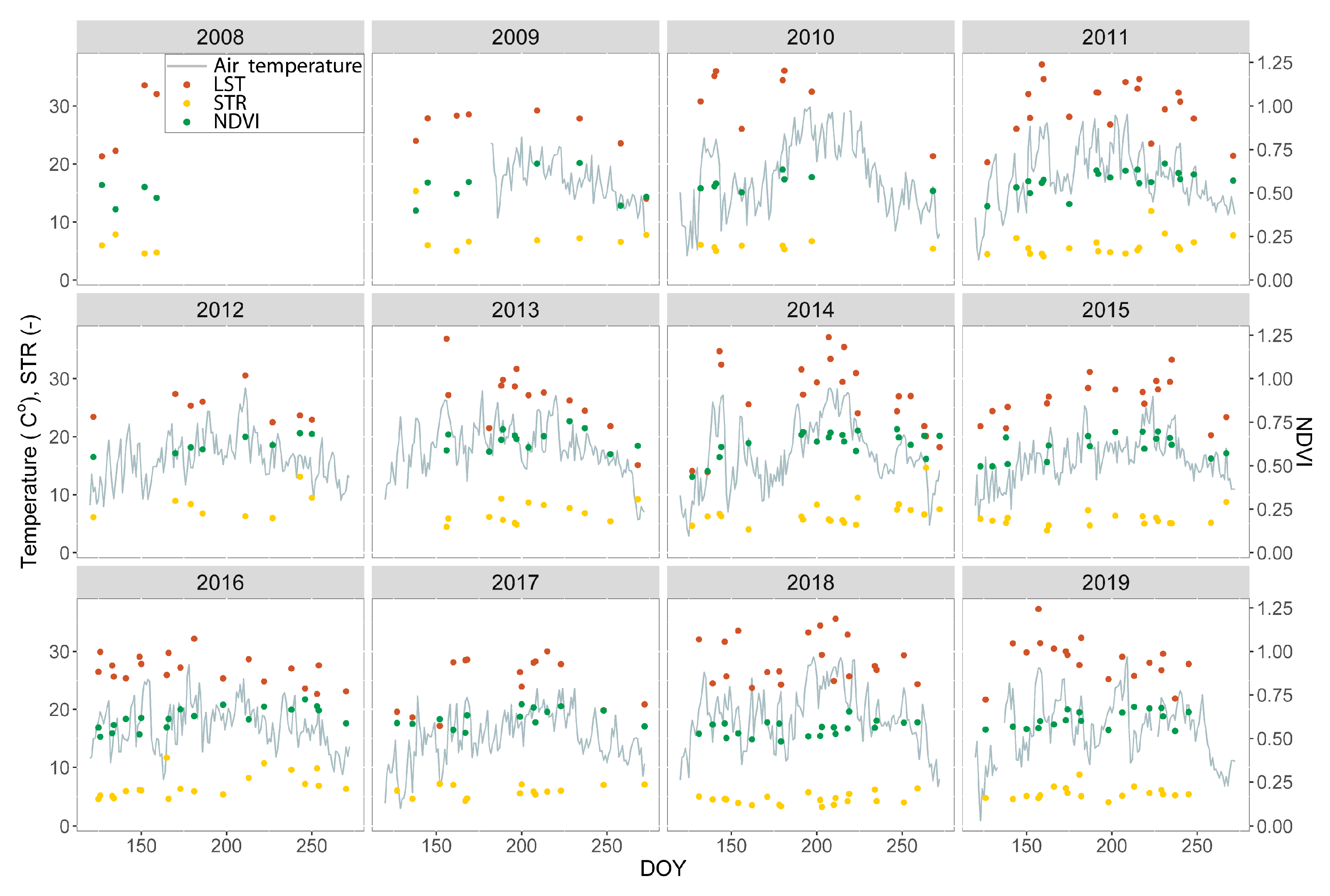
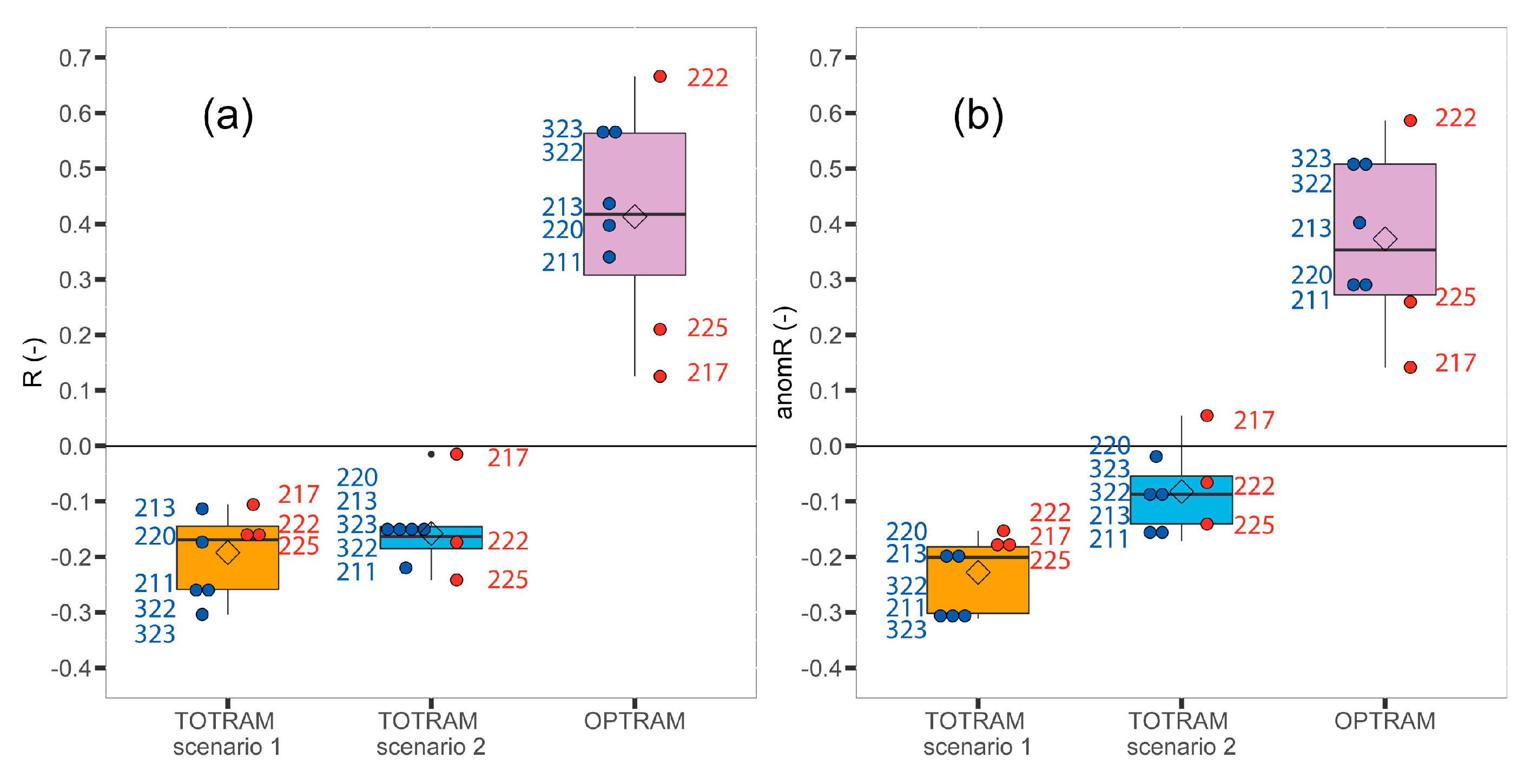
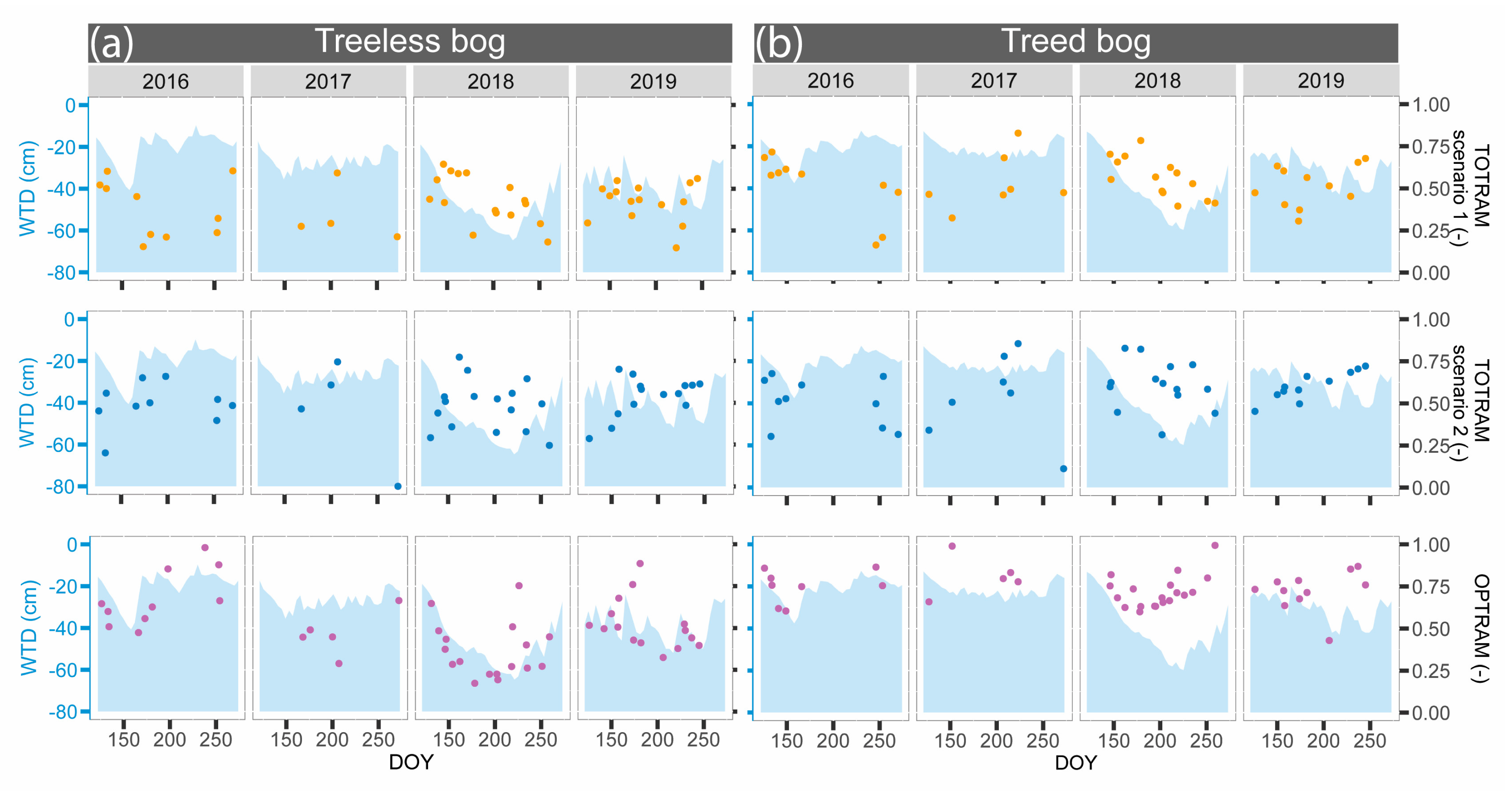
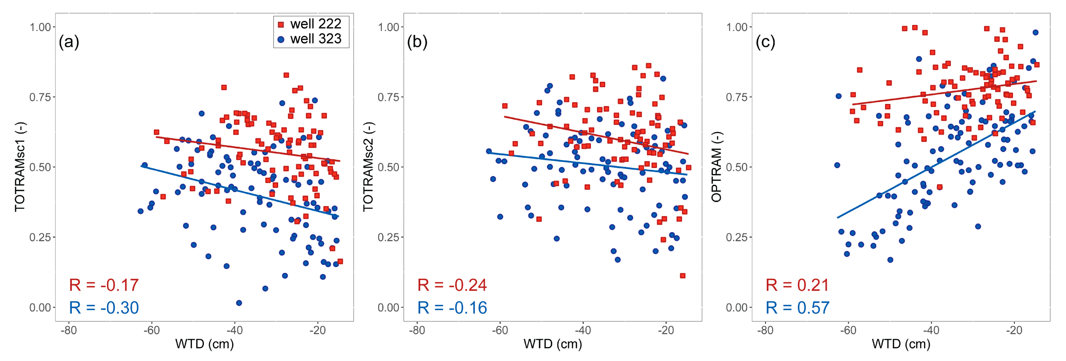
3.1. Temporal Correlation of Soil Moisture Indices with WTD

Figure 6 shows box plots (over eight wells) of the temporal correlation coefficients between WTD and soil moisture index estimated with two TOTRAM scenarios and OPTRAM as average values across four pixels closest to the wells. Both TOTRAM scenarios resulted in negative average R and anomR values of −0.19 and −0.23, respectively, for Scenario 1, and −0.16 and −0.08, respectively, for Scenario 2. In contrast, OPTRAM resulted in a weak positive R and anomR with average values of 0.41 and 0.37, respectively. The variability of R and anomR between the wells was also the highest for OPTRAM, with both low and high correlation values for the wells in the treed parts of the bog.
Figure 7 shows exemplarily time series for four of twelve years of WTD and the three different soil moisture indices. Time series are illustrated for monitoring wells 323 (treeless bog, Figure 7a) and 225 (treed bog, Figure 7b) as an average across four pixels closest to the wells. The WTD data highlights a fundamental relationship between WTD and vegetation type in bogs. Tree cover is an indicator of the deeper long-term WTD and higher temporal WTD variability [82].
As already indicated by the correlation coefficients, Figure 7 illustrates that the temporal variation of soil moisture indices estimated from TOTRAM Scenarios 1 and 2 does not agree with temporal changes in WTD. In contrast, the OPTRAM soil moisture index follows reasonably well the WTD dynamics, in particular in the treeless bog. However, some obvious outliers are still present.
As mentioned above, we observed high spatial correlation among the water levels measured in different monitoring wells. For the next analysis, we therefore assumed coherent fluctuations of WTD over the whole bog by calculating the mean WTD of the eight monitoring wells. We then analyzed the temporal correlation coefficient R between the mean WTD and the three different soil moisture indices for each individual Landsat pixel.
The resulting spatial differences in R were assumed to be dominated by the local specifics of the temporal relationship between the WTD and soil moisture index. Figure 8 shows that, for the two TOTRAM scenarios, the R values are close to zero. In contrast, R values of OPTRAM are positive throughout the whole bog area. The highest R values (up to 0.8) can be observed for treeless areas, where no pools and dwarf pines are present.

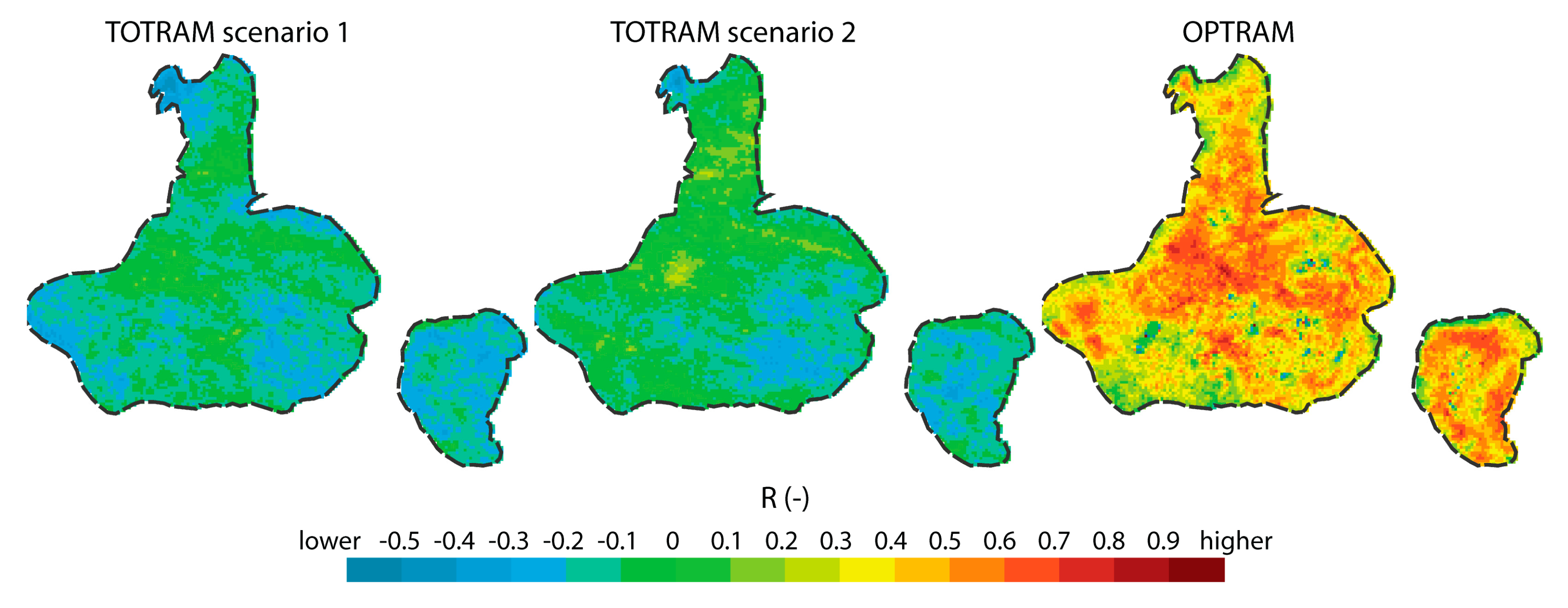
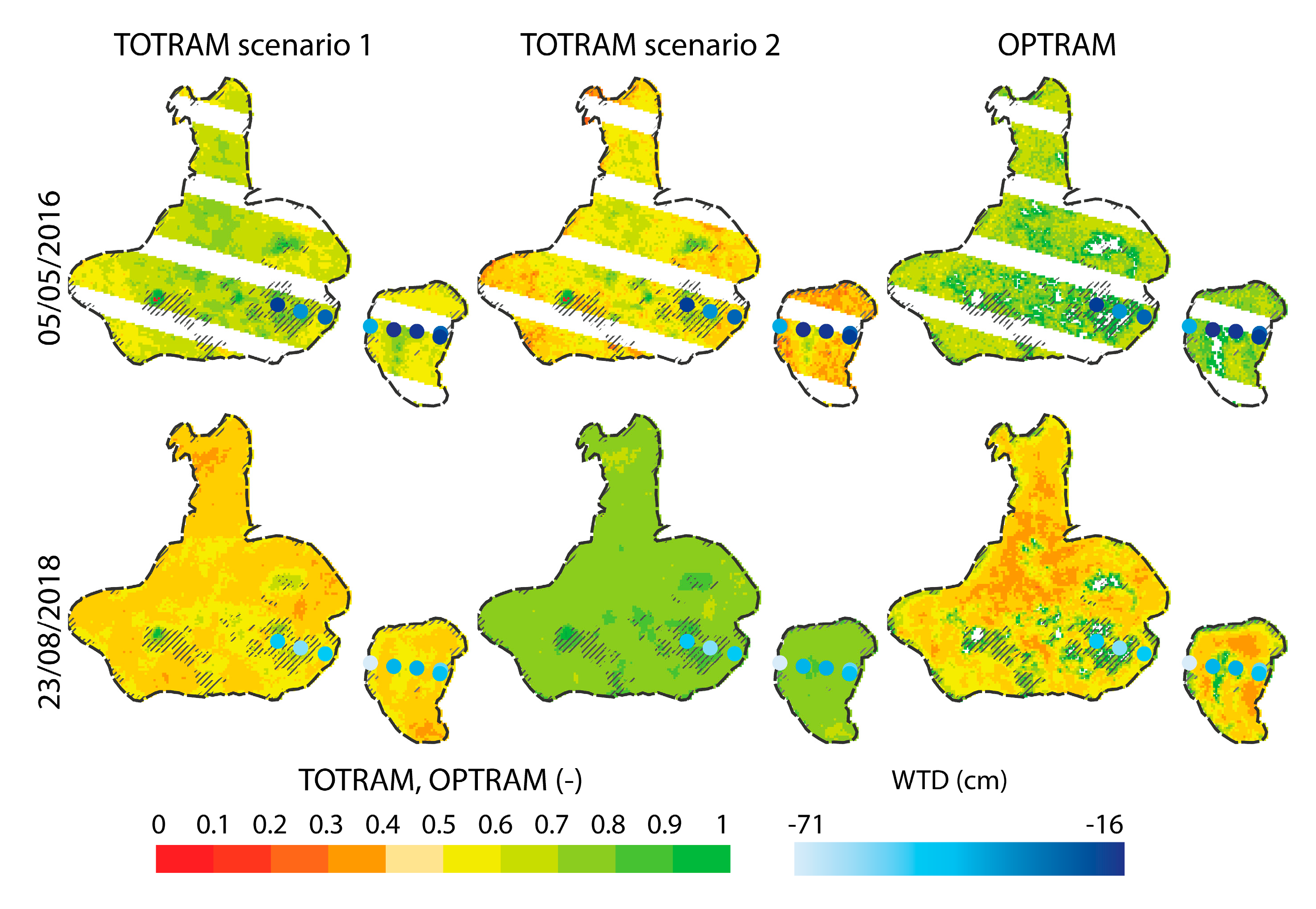
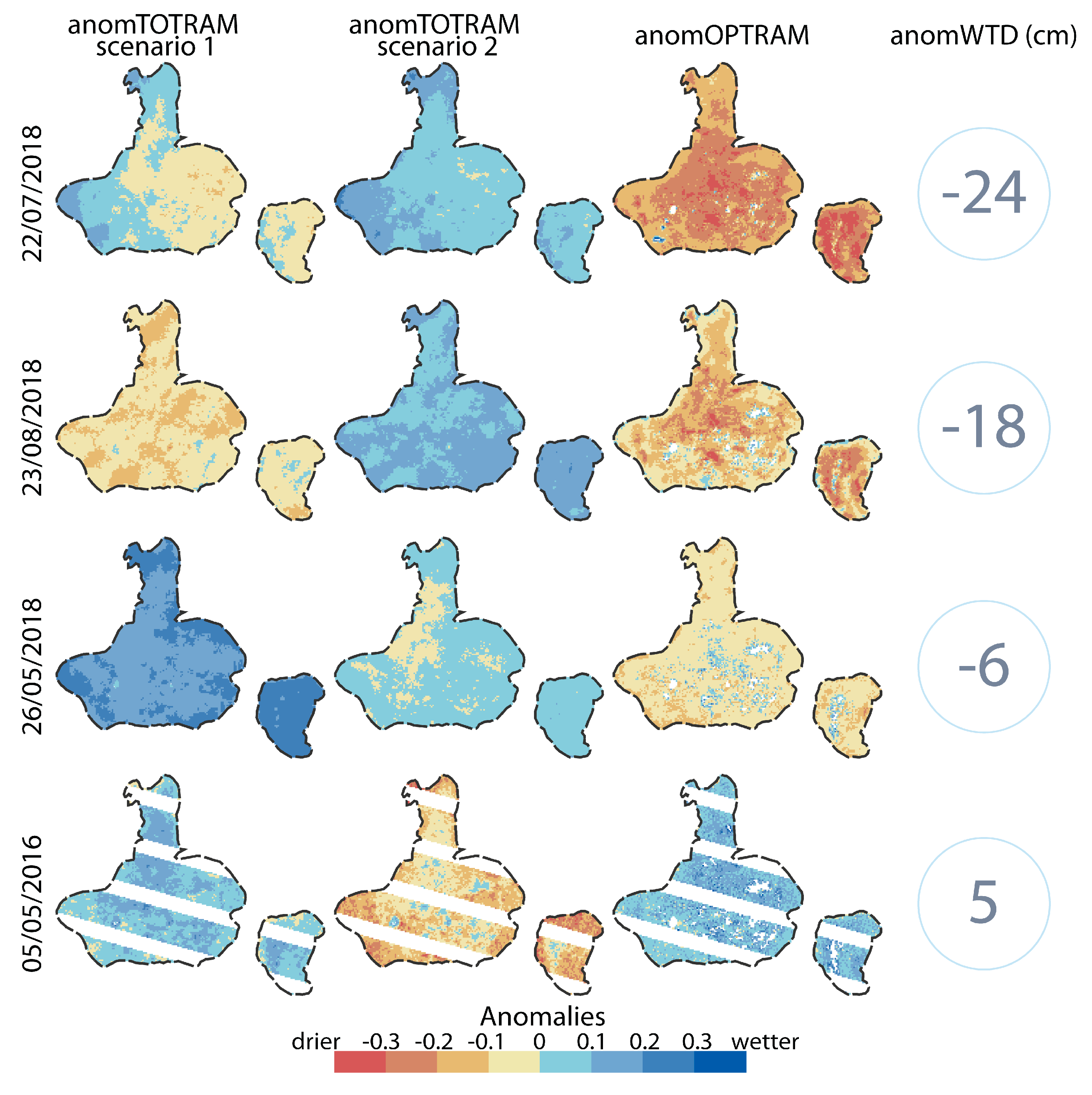
3.2. Spatial Variability of Soil Moisture Indices and WTD

Figure 9 shows scatterplots between the moisture indices and WTD across all times for two exemplary monitoring wells (same as in Figure 7): well 225 located in the treed part and well 323 located in the treeless part of the bogs. Figure 9a,b indicates that the soil moisture indices from both TOTRAM scenarios do not positively correlate with WTD. Only the OPTRAM index shows a positive correlation over the whole WTD range (Figure 9c). Furthermore, Figure 9c shows that OPTRAM values are systematically higher over treed parts of the bog and lower over treeless parts of the bog.
Figure 10 presents spatial patterns of soil moisture index generated by the two TOTRAM scenarios and OPTRAM for an exemplary wet (5 May 2016) and dry (23 August 2018) conditions. The TOTRAM Scenario 1 and OPTRAM indices indicate a basic agreement with in-situ WTD in terms of spatial averages of the two contrasting conditions. This is not the case for the TOTRAM Scenario 2 in which a wetter condition was indicated for the date with the dry condition. For this date, this was caused by a modeled dry edge that was too warm and therefore led to an underestimation of the TOTRAM Scenario 2 index.
None of the three methods was able to indicate plausible soil moisture variability. Under the dry conditions of the second date, the bogs typically show drier soil moisture and deeper WTD towards the margins. The opposite can be observed for OPTRAM, while TOTRAM does show very little variability. Furthermore, in-situ data of the second date indicated deepest WTD at wells 217 and 222, which are installed in the treed parts of the bogs. The OPTRAM index, however, did show relatively high values around those two wells.
Figure 11 shows maps of the anomaly time series of the soil moisture indices for four exemplary dates and the corresponding soil moisture anomaly averaged over all monitoring wells. In terms of spatial averages, there is again a good agreement between anomalies in WTD and OPTRAM index. In contrast, the TOTRAM scenarios did not yield changes that could be related to WTD.

4. Discussion

4.1. Lack of Correlation between TOTRAM Index and WTD

Given the strong linkage between soil moisture and WTD present in peatlands, a positive correlation between the TOTRAM soil moisture index and WTD was expected. However, such a positive correlation could not be observed for TOTRAM Scenario 1 or TOTRAM Scenario 2. Table 1 summarizes the limitations of TOTRAM approaches. Here, we emphasize two aspects of TOTRAM that hampered its applicability to our study area; both aspects are related to the generally wetter conditions in northern latitude ecosystems.
The most important limitation is that the TOTRAM indices are computed per scene. This limits the ability to sufficiently constrain the trapezoid space. The generally wetter conditions in northern latitudes may not sufficiently cover the range of moisture variability to properly constrain the trapezoid space. Our attempt to overcome this limitation by modeling a dry edge based on weather conditions (Scenario 2) did not improve the performance of TOTRAM.
A further possible reason for the lack (or even negative) correlation between WTD and TOTRAM indices might be that evapotranspiration and vegetation growth in northern latitudes are much more limited by energy than by moisture [100]. This likely leads to the violation of the assumption of TOTRAM that lower soil moistures lead to an increase in LST. Karnieli et al. [101] showed that LST and VI can have a positive association in the area where vegetation growth is limited by energy. For example, in high latitude regions, warming is accompanied by vegetation growth and, thus, an LST increase cannot be a reliable indicator of vegetation stress. Garcia et al. [102] demonstrated that this is a limitation of TOTRAM and suggested to apply it only to the regions where water and not energy is limiting. Further research should investigate the applicability of TOTRAM for the WTD monitoring in peatlands of climatic zones for which energy is not a limiting factor of vegetation growth (Table 1).

4.2. Potential and Challenges of Using OPTRAM for WTD Monitoring

Our results demonstrate a high potential of the OPTRAM index to monitor temporal changes of WTD dynamics in northern bogs. The average correlation coefficients were as high as the ones obtained for radar backscatter coefficient over natural peatlands in an earlier study [38]. Especially over treeless areas, correlation coefficients achieved with OPTRAM index were very promising and reached values up to 0.8. The good temporal correlation statistics suggests that OPTRAM index might be a new type of observation suitable for assimilation into peatland-specific hydrological models [33].
However, a closer investigation of the local time series showed some obvious outliers. The identification of the reasons for these outliers and methods to filter such data will be critical to increase the applicability of the OPTRAM index for WTD monitoring in peatlands. Most importantly, it is possible that the OPTRAM index represents more or less the vegetation status or the soil moisture at various depths at different times. As OPTRAM relies on the dependency of the SWIR reflectance on plant moisture content, the soil depth dependency needs to be developed for different vegetation types and their typical rooting depths.
Similar to the microwave backscatter signal and coherence, the spatial variation of the OPTRAM index is highly influenced by the vegetation patterns [38,103]. For our study area, the simple differentiation into treed (covered with dwarf pines) and treeless (covered mainly with Sphagnum mosses) bog areas showed that vegetation variability was the dominating factor controlling spatial variability of the OPTRAM index. The importance of vegetation types and leaf internal structure of different species likely goes beyond such a coarse differentiation of vegetation types [44,70] as indicated by the large variance of the OPTRAM index within the treeless and treed areas (Figure 9). This variance is likely attributed to the differences in SWIR reflectance of species within one genus. For example, differently structured Sphagnum species have uneven ability to retain water under the same environmental conditions; thus, their behavior in the SWIR channel varies [104,105,106,107,108,109].
The high OPTRAM dependency on vegetation cover warrants a note of caution for its use in long-term monitoring studies (Table 1). Vegetation types and specific species communities can vary a lot in time in reaction to long-term changes of WTD [110]. This limitation is an important issue for future research, because the long Landsat record would be of particular interest for such a long-term monitoring of moisture changes in peatlands due to climate change or human disturbance. By now, it has been suggested combining SWIR channel data with NIR data to minimize the uncertainty in the estimation of soil moisture for different vegetation cover [44]. In further studies, it should be tried to integrate the NIR channel into the OPTRAM approach.
Finally, it should be reiterated that the WTD estimation with OPTRAM is successful here, mainly because of the strong vertical coupling of surface (and root-zone) soil moisture with the typical shallow WTD over bogs. It is unlikely (but not tested) that the method would perform as well in areas with deep WTD or mineral soil properties.

5. Conclusions

We evaluated the temporal and spatial relationships between in-situ measured WTD and soil moisture indices from three different trapezoid models over two northern bogs in Estonia. We compared the performance of two trapezoid models based on optical and thermal imagery (TOTRAM Scenarios 1 and 2) and one solely based on optical imagery (OPTRAM). Our results demonstrate:
  • a general inapplicability of the TOTRAM index for the spatial and temporal WTD monitoring in our study area;
  • a high potential of OPTRAM index for monitoring temporal changes in WTD with average temporal Pearson correlation coefficients of 0.41 for original and 0.37 for anomaly time series;
  • the highest temporal correlation coefficients (0.8) for the OPTRAM index over treeless bog areas with little or no surface water (no bog pools); and
  • a high sensitivity of OPTRAM index to the vegetation type. Together with unknown spatial variability of the soil moisture–WTD relationship, this strongly limits the spatial interpretability and probably also the long-term temporal interpretability of the OPTRAM index for WTD monitoring under progressive changes of vegetation and peat properties.
The present study provides the first comprehensive assessment of the potential of TOTRAM and OPTRAM to monitor WTD dynamics over two selected northern bogs. Further studies are necessary to assess the performance over other peatlands in northern as well as tropical regions. Further research should be undertaken to improve the accuracy of OPTRAM and minimize the uncertainties caused by the differences in vegetation cover.

Author Contributions

Conceptualization, I.B., M.B., and V.S.; Data curation, I.B.; Formal analysis, I.B. and M.B.; Funding acquisition, V.S. and Ü.M.; Investigation, I.B. and M.B.; Methodology, I.B. and M.B.; Project administration, M.B., V.S., G.D.L., and Ü.M.; Resources, G.D.L. and Ü.M.; Software, I.B. and V.K.; Supervision, M.B., V.S., G.D.L., and Ü.M.; Validation, I.B. and M.B.; Visualization, I.B., and M.B.; Writing—original draft, I.B.; and Writing—review and editing, M.B., V.S., G.D.L., and Ü.M. All authors have read and agreed to the published version of the manuscript.

Funding

This research was funded by the European Social Fund’s Dora Plus Programme, grant number 36.9-6.1/1222, the Ministry of Education and Science of Estonia, grants numbers IUT2-16 and PRG352, and the EU through European Regional Development Fund for the Centre of Excellence “Ecology of Global Change: Natural and Managed Ecosystems” (EcolChange), grant number is not applicable. M. Bechtold thanks the Alexander von Humboldt Foundation for a Feodor Lynen Fellowship.

Acknowledgments

We are grateful to the staff of the Tooma mire research station, who provided hydrometeorological data for this study.

Conflicts of Interest

The authors declare no conflict of interest. The funders had no role in the design of the study; in the collection, analyses, or interpretation of data; in the writing of the manuscript, or in the decision to publish the results.

Appendix A

Estimation of the temperature of the driest bare surface (LSTsmax)
Following the two-source model described in [55], LSTsmax could be implicit in radiation budget and energy balance equations for the driest bare soil surface which does not evaporate:
R s = ( 1 α s ) S d + ( L d L u ) ( 1 ε s ) L d = ( 1 α s ) S d + ε s L d L u = ( 1 α s ) S d + ε s ε a σ T a 4 ε s σ L S T s 4
R s G = H s + L E s = ρ c p ( L S T s T a r a , s ) + L E s
L S T s m a x = R s 4 ε s σ T a 3 + ρ c p [ r a , s ( 1 c ) ] + T a
where Rs is the net radiation of soil surface (W m−2); αs is the albedo for the soil surface (unitless); Sd is the downwelling shortwave radiation (W m−2); Ld and Lu are the downwelling and upwelling longwave radiation (W m−2); εs is the broadband emissivity of the soil surface (unitless); εa is the emissivity of the atmosphere (unitless); ρ is the air density (kg m−3); cp is the air specific heat at the constant pressure taken as 1.013 × 10³ (J kg−1 K−1) [111]; ra,s is the aerodynamic resistance of the bare soil surface (s m−1); σ is the Stefan–Boltzmann constant 5.67 × 10⁻⁸ (kg s−3 K−4); c is the calibrated proportionality coefficient equal to 0.35 (unitless); Ta is the air temperature (K); and LEs is the evaporation from soil surface (W m−2).
The aerodynamic resistance for the bare soil surface could be calculated in the following way:
r a , s = 1 0.0015 u 1 m
where u1m is the wind velocity at the height of 1 m above the bare soil surface (m s−1), which can be estimated from the logarithmic wind profile function:
u 1 m = u * k ( ln ( z m d ) z o m φ m ( z m ) + φ m ( z o m ) )
where u* is the friction velocity (m s−1); k is the von Karman’s constant equal to 0.41 (unitless); zm is the reference height of the wind velocity measurements, which is taken as 1 m; d is the zero plane displacement taken as 0 m; zom is the roughness length for momentum transfer assumed to be 0.005 m [112]; and φm(zm) and φm(zom) are the factors used for the stability correction at 1 m and 0.005 m height (unitless), which depend on the Monin–Obukhov length L (m) and can be expressed for the stable conditions (L > 0) as follows:
φ m ( z m ) = 5 ( 1 L )
φ m ( z o m ) = 5 ( z o m L )
For the unstable conditions (L < 0), factors are calculated in the following way:
φ m ( 1 ) = 2 ln ( 1 + x ( 1 ) 2 ) + ln ( 1 + x ( 1 ) 2 2 ) 2 arctan ( x ( 1 ) ) + 0.5 π
φ m ( z o m ) = 2 ln ( 1 + x ( z o m ) 2 ) + ln ( 1 + x ( z o m ) 2 2 ) 2 arctan ( x ( z o m ) ) + 0.5 π
x ( 1 ) = ( 1 16 1 L ) 0.25
x ( z o m ) = ( 1 16 z o m L ) 0.25
where L is calculated as follows:
L = ρ c p u * 3 T a k g H s
where g is gravitational acceleration taken as 9.8 (m s−2).
Finally, LSTsmax can be obtained iteratively using Equations (A1)–(A4) and (A7).

Appendix B

Estimation of the temperature of the driest fully vegetated surface (LSTcmax)
In a similar way, Long et al. [55] suggested calculating LSTcmax from the radiative budget equation:
R c = ( 1 α c ) S d + ( L d L u ) ( 1 ε c ) L d = ( 1 α c ) S d + ε c L d L u = ( 1 α c ) S d + ε c ε a σ T a 4 ε c σ L S T c 4
R c = H c + L E c = ρ c p ( L S T c T a r a , c ) + L E c
L S T c m a x = R c 4 ε c σ T a 3 + ρ c p r a , s + T a
where Rc is the net radiation of fully vegetated surface (W m−2); αc is the albedo for vegetation (unitless); εc is the broadband emissivity of vegetation (unitless); LEc is the evaporation from vegetation (W m−2); and ra,c is the aerodynamic resistance above the canopy surface (s m−1) expressed as follows:
r a , c = ln ( z T d z o h ) φ h ( z T ) + φ h ( z o h ) u * k
where u* is calculated following Equation (A5), but φm(zm) and φm(zom) for the stable condition (L > 0) are calculated in the following way:
φ m ( z m ) = 5 ( z m L )
φ m ( z o m ) = 5 ( z o m L )
φ h ( z T ) = 5 ( z T L )
φ h ( z o h ) = 5 ( z o h L )
For the unstable condition (L < 0), φm(zm) and φm(zom) are:
φ m ( z m ) = 2 ln ( 1 + x ( z m ) 2 ) + ln ( 1 + x ( z m ) 2 2 ) 2 arctan ( x ( z m ) ) + 0.5 π
φ m ( z o m ) = 2 ln ( 1 + x ( z o m ) 2 ) + ln ( 1 + x ( z o m ) 2 2 ) 2 arctan ( x ( z o m ) ) + 0.5 π
φ h ( z T ) = 2 ln ( 1 + x ( z T ) 2 2 )
φ h ( z o h ) = 2 ln ( 1 + x ( z o h ) 2 2 )
x ( z m ) = ( 1 16 z m L ) 0.25
x ( z o m ) = ( 1 16 z o m L ) 0.25
x ( z T ) = ( 1 16 z T L ) 0.25
x ( z o h ) = ( 1 16 z o h L ) 0.25
where zT is the reference height for temperature measurements assumed to be 2 m and the vegetation height is hc = 1 m; and d, zom, and zoh are taken as:
d = 2 h c 3
z o m = h c 10
z o h = z o m 7
LSTcmax can be derived by solving for the system of Equations (A13)–(A15) and (A20).

References

  1. Thompson, R.L.; Sasakawa, M.; Machida, T.; Aalto, T.; Worthy, D.; Lavric, J.V.; Lund Myhre, C.; Stohl, A. Methane fluxes in the high northern latitudes for 2005–2013 estimated using a Bayesian atmospheric inversion. Atmos. Chem. Phys. 2017, 17, 3553–3572. [Google Scholar] [CrossRef] [Green Version]
  2. Chen, X.; Wang, G.; Zhang, T.; Mao, T.; Wei, D.; Song, C.; Hu, Z.; Huang, K. Effects of warming and nitrogen fertilization on GHG flux in an alpine swamp meadow of a permafrost region. Sci. Total Environ. 2017, 601–602, 1389–1399. [Google Scholar] [CrossRef] [PubMed]
  3. Helbig, M.; Chasmer, L.E.; Desai, A.R.; Kljun, N.; Quinton, W.L.; Sonnentag, O. Direct and indirect climate change effects on carbon dioxide fluxes in a thawing boreal forest-wetland landscape. Glob. Chang. Biol. 2017, 23, 3231–3248. [Google Scholar] [CrossRef] [PubMed] [Green Version]
  4. Luo, Y.; Ahlström, A.; Allison, S.D.; Batjes, N.H.; Brovkin, V.; Carvalhais, N.; Chappell, A.; Ciais, P.; Davidson, E.A.; Finzi, A.; et al. Toward more realistic projections of soil carbon dynamics by Earth system models. Glob. Biogeochem. Cycles 2016, 30, 40–56. [Google Scholar] [CrossRef]
  5. Moore, T.R.; Bubier, J.L.; Frolking, S.E.; Lafleur, P.M.; Roulet, N.T. Plant biomass and production and CO2 exchange in an ombrotrophic bog. J. Ecol. 2002, 90, 25–36. [Google Scholar] [CrossRef]
  6. Gorham, E. Northern Peatlands: Role in the Carbon Cycle and Probable Responses to Climatic Warming. Ecol. Appl. 1991, 1, 182–195. [Google Scholar] [CrossRef]
  7. Lafleur, P.M.; Moore, T.R.; Roulet, N.T.; Frolking, S. Ecosystem Respiration in a Cool Temperate Bog Depends on Peat Temperature But Not Water Table. Ecosystems 2005, 8, 619–629. [Google Scholar] [CrossRef]
  8. Salm, J.-O.; Maddison, M.; Tammik, S.; Soosaar, K.; Truu, J.; Mander, Ü. Emissions of CO2, CH4 and N2O from undisturbed, drained and mined peatlands in Estonia. Hydrobiologia 2012, 692, 41–55. [Google Scholar] [CrossRef]
  9. Alm, J.; Schulman, L.; Walden, J.; Nykanen, H.; Martikainen, P.J.; Silvola, J. Carbon Balance of a Boreal Bog during a Year with an Exceptionally Dry Summer. Ecology 1999, 80, 161. [Google Scholar] [CrossRef]
  10. Pärn, J.; Verhoeven, J.T.A.; Butterbach-Bahl, K.; Dise, N.B.; Ullah, S.; Aasa, A.; Egorov, S.; Espenberg, M.; Järveoja, J.; Jauhiainen, J.; et al. Nitrogen-rich organic soils under warm well-drained conditions are global nitrous oxide emission hotspots. Nat. Commun. 2018, 9, 1135. [Google Scholar] [CrossRef] [Green Version]
  11. Schindler, U.; Müller, L. Simplifying the evaporation method for quantifying soil hydraulic properties. J. Plant Nutr. Soil Sci. 2006, 169, 623–629. [Google Scholar] [CrossRef]
  12. Weiss, R.; Alm, J.; Laiho, R.; Laine, J. Modeling Moisture Retention in Peat Soils. Soil Sci. Soc. Am. J. 1998, 62, 305. [Google Scholar] [CrossRef]
  13. Lehmann, P.; Assouline, S.; Or, D. Characteristic lengths affecting evaporative drying of porous media. Phys. Rev. E Stat. NonlinearSoft Matter Phys. 2008, 77, 056309. [Google Scholar] [CrossRef] [PubMed]
  14. Sadeghi, M.; Shokri, N.; Jones, S.B. A novel analytical solution to steady-state evaporation from porous media. Water Resour. Res. 2012, 48. [Google Scholar] [CrossRef] [Green Version]
  15. Rezanezhad, F.; Price, J.S.; Quinton, W.L.; Lennartz, B.; Milojevic, T.; Van Cappellen, P. Structure of peat soils and implications for water storage, flow and solute transport: A review update for geochemists. Chem. Geol. 2016, 429, 75–84. [Google Scholar] [CrossRef]
  16. Cagampan, J.P.; Waddington, J.M. Moisture dynamics and hydrophysical properties of a transplanted acrotelm on a cutover peatland. Hydrol. Process. 2008, 22, 1776–1787. [Google Scholar] [CrossRef] [Green Version]
  17. Holden, J.; Burt, T.P.; Cox, N.J. Macroporosity and infiltration in blanket peat: The implications of tension disc infiltrometer measurements. Hydrol. Process. 2001, 15, 289–303. [Google Scholar] [CrossRef]
  18. Chason, D.B.; Siegel, D.I. Hydraulic conductivity and related physical properties of peat, lost river peatland, northern minnesota. Soil Sci. 1986, 142, 91–99. [Google Scholar] [CrossRef]
  19. Lindholm, T.; Markkula, I. Moisture conditions in hummocks and hollows in virgin and drained sites on the raised bog Laaviosuo, southern Finland. Ann. Bot. Fenn. 1984, 21, 241–255. [Google Scholar]
  20. Price, J. Soil moisture, water tension, and water table relationships in a managed cutover bog. J. Hydrol. 1997, 202, 21–32. [Google Scholar] [CrossRef]
  21. Price, J.S.; Schlotzhauer, S.M. Importance of shrinkage and compression in determining water storage changes in peat: The case of a mined peatland. Hydrol. Process. 1999, 13, 2591–2601. [Google Scholar] [CrossRef] [Green Version]
  22. Kellner, E.; Halldin, S. Water budget and surface-layer water storage in a Sphagnum bog in central Sweden. Hydrol. Process. 2002, 16, 87–103. [Google Scholar] [CrossRef]
  23. Strack, M.; Price, J.S. Moisture controls on carbon dioxide dynamics of peat-Sphagnum monoliths. Ecohydrology 2009, 2, 34–41. [Google Scholar] [CrossRef]
  24. Kull, A.; Kull, A.; Jaagus, J.; Kuusemets, V.; Mander, Ü. The Effects of Fluctuating Climatic Conditions and Weather Events on Nutrient Dynamics in a Narrow Mosaic Riparian Peatland. Boreal Environ. Res. 2008, 13, 243–263. [Google Scholar]
  25. Kerr, Y.H.; Waldteufel, P.; Wigneron, J.P.; Delwart, S.; Cabot, F.; Boutin, J.; Escorihuela, M.J.; Font, J.; Reul, N.; Gruhier, C.; et al. The SMOS L: New tool for monitoring key elements ofthe global water cycle. Proc. IEEE 2010, 98, 666–687. [Google Scholar] [CrossRef] [Green Version]
  26. Entekhabi, D.; Njoku, E.G.; O’Neill, P.E.; Kellogg, K.H.; Crow, W.T.; Edelstein, W.N.; Entin, J.K.; Goodman, S.D.; Jackson, T.J.; Johnson, J.; et al. The soil moisture active passive (SMAP) mission. Proc. IEEE 2010, 98, 704–716. [Google Scholar] [CrossRef]
  27. Ulaby, F.; Long, D. Microwave Radar and Radiometric Remote Sensing; University of Michigan Press: Ann Arbor, MI, USA, 2014; ISBN 978-0-472-11935-6. [Google Scholar]
  28. Dorigo, W.; Wagner, W.; Albergel, C.; Albrecht, F.; Balsamo, G.; Brocca, L.; Chung, D.; Ertl, M.; Forkel, M.; Gruber, A.; et al. ESA CCI Soil Moisture for improved Earth system understanding: State-of-the art and future directions. Remote Sens. Environ. 2017, 203, 185–215. [Google Scholar] [CrossRef]
  29. Bauer-Marschallinger, B.; Freeman, V.; Cao, S.; Paulik, C.; Schaufler, S.; Stachl, T.; Modanesi, S.; Massari, C.; Ciabatta, L.; Brocca, L.; et al. Toward Global Soil Moisture Monitoring with Sentinel-1: Harnessing Assets and Overcoming Obstacles. IEEE Trans. Geosci. Remote Sens. 2019, 57, 520–539. [Google Scholar] [CrossRef]
  30. Asmuß, T.; Bechtold, M.; Tiemeyer, B. On the Potential of Sentinel-1 for High Resolution Monitoring of Water Table Dynamics in Grasslands on Organic Soils. Remote Sens. 2019, 11, 1659. [Google Scholar] [CrossRef] [Green Version]
  31. Bircher, S.; Demontoux, F.; Razafindratsima, S.; Zakharova, E.; Drusch, M.; Wigneron, J.-P.; Kerr, Y. L-Band Relative Permittivity of Organic Soil Surface Layers—A New Dataset of Resonant Cavity Measurements and Model Evaluation. Remote Sens. 2016, 8, 1024. [Google Scholar] [CrossRef] [Green Version]
  32. Jonard, F.; Bircher, S.; Demontoux, F.; Weihermüller, L.; Razafindratsima, S.; Wigneron, J.-P.; Vereecken, H. Passive L-Band Microwave Remote Sensing of Organic Soil Surface Layers: A Tower-Based Experiment. Remote Sens. 2018, 10, 304. [Google Scholar] [CrossRef] [Green Version]
  33. Bechtold, M.; De Lannoy, G.; Reichle, R.H.; Roose, D.; Balliston, N.; Burdun, I.; Devito, K.; Kurbatova, J.; Munir, T.M.; Zarov, E.A. Improved Groundwater Table and L-band Brightness Temperature Estimates for Northern Hemisphere Peatlands Using New Model Physics and SMOS Observations in a Global Data Assimilation Framework. Remote Sens. Environ. 2020, 246. [Google Scholar] [CrossRef]
  34. Dabrowska-Zielinska, K.; Budzynska, M.; Tomaszewska, M.; Malinska, A.; Gatkowska, M.; Bartold, M.; Malek, I. Assessment of Carbon Flux and Soil Moisture in Wetlands Applying Sentinel-1 Data. Remote Sens. 2016, 8, 756. [Google Scholar] [CrossRef] [Green Version]
  35. Chen, Z.; White, L.; Banks, S.; Behnamian, A.; Montpetit, B.; Pasher, J.; Duffe, J.; Bernard, D. Characterizing marsh wetlands in the Great Lakes Basin with C-band InSAR observations. Remote Sens. Environ. 2020, 242, 111750. [Google Scholar] [CrossRef]
  36. Ulaby, F.T.; Moore, R.K.; Fung, A.K. Microwave Remote Sensing: Active and Passive; Artech House: Norwood, MA, USA, 1981; ISBN 0890061904. [Google Scholar]
  37. Wagner, W.; Lemoine, G.; Borgeaud, M.; Rott, H. A study of vegetation cover effects on ers scatterometer data. IEEE Trans. Geosci. Remote Sens. 1999, 37, 938–948. [Google Scholar] [CrossRef]
  38. Bechtold, M.; Schlaffer, S.; Tiemeyer, B.; De Lannoy, G. Inferring Water Table Depth Dynamics from ENVISAT-ASAR C-Band Backscatter over a Range of Peatlands from Deeply-Drained to Natural Conditions. Remote Sens. 2018, 10, 536. [Google Scholar] [CrossRef] [Green Version]
  39. Bourgeau-Chavez, L.L.; Kasischke, E.S.; Riordan, K.; Brunzell, S.; Nolan, M.; Hyer, E.; Slawski, J.; Medvecz, M.; Walters, T.; Ames, S. Remote monitoring of spatial and temporal surface soil moisture in fire disturbed boreal forest ecosystems with ERS SAR imagery. Int. J. Remote Sens. 2007, 28, 2133–2162. [Google Scholar] [CrossRef]
  40. Zwieback, S.; Berg, A.A. Fine-Scale SAR Soil Moisture Estimation in the Subarctic Tundra. IEEE Trans. Geosci. Remote Sens. 2019, 57, 4898–4912. [Google Scholar] [CrossRef]
  41. Tang, R.; Li, Z.-L.; Tang, B. An application of the Ts–VI triangle method with enhanced edges determination for evapotranspiration estimation from MODIS data in arid and semi-arid regions: Implementation and validation. Remote Sens. Environ. 2010, 114, 540–551. [Google Scholar] [CrossRef]
  42. Sandholt, I.; Rasmussen, K.; Andersen, J. A simple interpretation of the surface temperature/vegetation index space for assessment of surface moisture status. Remote Sens. Environ. 2002, 79, 213–224. [Google Scholar] [CrossRef]
  43. Wardlow, B.D.; Anderson, M.C.; Verdin, J.P. Remote Sensing of Drought: Innovative Monitoring Approaches; CRC Press: Boca Raton, FL, USA, 2012; ISBN 9781138075207. [Google Scholar]
  44. Sadeghi, M.; Babaeian, E.; Tuller, M.; Jones, S.B. The optical trapezoid model: A novel approach to remote sensing of soil moisture applied to Sentinel-2 and Landsat-8 observations. Remote Sens. Environ. 2017, 198, 52–68. [Google Scholar] [CrossRef] [Green Version]
  45. Goward, S.N.; Cruickshanks, G.D.; Hope, A.S. Observed relation between thermal emission and reflected spectral radiance of a complex vegetated landscape. Remote Sens. Environ. 1985, 18, 137–146. [Google Scholar] [CrossRef]
  46. Carlson, T. An Overview of the Triangle Method for Estimating Surface Evapotranspiration and Soil Moisture from Satellite Imagery. Sensors 2007, 7, 1612–1629. [Google Scholar] [CrossRef] [Green Version]
  47. Carlson, T.N.; Gillies, R.R.; Perry, E.M. A method to make use of thermal infrared temperature and NDVI measurements to infer surface soil water content and fractional vegetation cover. Remote Sens. Rev. 1994, 9, 161–173. [Google Scholar] [CrossRef]
  48. Moran, M.S.; Clarke, T.R.; Inoue, Y.; Vidal, A. Estimating crop water deficit using the relation between surface-air temperature and spectral vegetation index. Remote Sens. Environ. 1994, 49, 246–263. [Google Scholar] [CrossRef]
  49. El Hajj, M.; Baghdadi, N.; Zribi, M.; Bazzi, H.; El Hajj, M.; Baghdadi, N.; Zribi, M.; Bazzi, H. Synergic Use of Sentinel-1 and Sentinel-2 Images for Operational Soil Moisture Mapping at High Spatial Resolution over Agricultural Areas. Remote Sens. 2017, 9, 1292. [Google Scholar] [CrossRef] [Green Version]
  50. Carlson, T.N.; Petropoulos, G.P. A new method for estimating of evapotranspiration and surface soil moisture from optical and thermal infrared measurements: The simplified triangle. Int. J. Remote Sens. 2019, 40, 7716–7729. [Google Scholar] [CrossRef]
  51. Wang, W.; Huang, D.; Wang, X.-G.; Liu, Y.-R.; Zhou, F. Hydrology and Earth System Sciences Estimation of soil moisture using trapezoidal relationship between remotely sensed land surface temperature and vegetation index. Hydrol. Earth Syst. Sci. 2011, 15, 1699–1712. [Google Scholar] [CrossRef] [Green Version]
  52. Patel, N.R.; Anapashsha, R.; Kumar, S.; Saha, S.K.; Dadhwal, V.K. Assessing potential of MODIS derived temperature/vegetation condition index (TVDI) to infer soil moisture status. Int. J. Remote Sens. 2009, 30, 23–39. [Google Scholar] [CrossRef]
  53. Mallick, K.; Bhattacharya, B.K.; Patel, N.K. Estimating volumetric surface moisture content for cropped soils using a soil wetness index based on surface temperature and NDVI. Agric. Meteorol. 2009, 149, 1327–1342. [Google Scholar] [CrossRef]
  54. Goward, S.N.; Xue, Y.; Czajkowski, K.P. Evaluating land surface moisture conditions from the remotely sensed temperature/vegetation index measurements: An exploration with the simplified simple biosphere model. Remote Sens. Environ. 2002, 79, 225–242. [Google Scholar] [CrossRef]
  55. Long, D.; Singh, V.P. A Two-source Trapezoid Model for Evapotranspiration (TTME) from satellite imagery. Remote Sens. Environ. 2012, 121, 370–388. [Google Scholar] [CrossRef]
  56. Yang, Y.; Su, H.; Zhang, R.; Tian, J.; Li, L. An enhanced two-source evapotranspiration model for land (ETEML): Algorithm and evaluation. Remote Sens. Environ. 2015, 168, 54–65. [Google Scholar] [CrossRef]
  57. Ambrosone, M.; Matese, A.; Di Gennaro, S.F.; Gioli, B.; Tudoroiu, M.; Genesio, L.; Miglietta, F.; Baronti, S.; Maienza, A.; Ungaro, F.; et al. Retrieving soil moisture in rainfed and irrigated fields using Sentinel-2 observations and a modified OPTRAM approach. Int. J. Appl. Earth Obs. Geoinf. 2020, 89, 102113. [Google Scholar] [CrossRef]
  58. Babaeian, E.; Sadeghi, M.; Franz, T.E.; Jones, S.; Tuller, M. Mapping soil moisture with the OPtical TRApezoid Model (OPTRAM) based on long-term MODIS observations. Remote Sens. Environ. 2018, 211, 425–440. [Google Scholar] [CrossRef]
  59. Huang, F.; Wang, P.; Ren, Y.; Liu, R. Estimating Soil Moisture Using the Optical Trapezoid Model (OPTRAM) in a Semi-Arid Area of SONGNEN Plain, China Based on Landsat-8 Data. In Proceedings of the International Geoscience and Remote Sensing Symposium (IGARSS); Institute of Electrical and Electronics Engineers Inc.: Yokohama, Japan, 2019; pp. 7010–7013. [Google Scholar]
  60. Chen, M.; Zhang, Y.; Yao, Y.; Lu, J.; Pu, X.; Hu, T.; Wang, P. Evaluation of an OPtical TRApezoid Model (OPTRAM) to retrieve soil moisture in the Sanjiang Plain of Northeast China. Earth Sp. Sci. 2020. [Google Scholar] [CrossRef]
  61. Klinke, R.; Kuechly, H.; Frick, A.; Förster, M.; Schmidt, T.; Holtgrave, A.K.; Kleinschmit, B.; Spengler, D.; Neumann, C. Indicator-Based Soil Moisture Monitoring of Wetlands by Utilizing Sentinel and Landsat Remote Sensing Data. PFG J. Photogramm. Remote Sens. Geoinf. Sci. 2018, 86, 71–84. [Google Scholar] [CrossRef]
  62. Zhang, D.; Tang, R.; Tang, B.H.; Wu, H.; Li, Z.L. A simple method for soil moisture determination from LST-VI feature space using nonlinear interpolation based on thermal infrared remotely sensed data. IEEE J. Sel. Top. Appl. Earth Obs. Remote Sens. 2015, 8, 638–648. [Google Scholar] [CrossRef]
  63. Capodici, F.; Cammalleri, C.; Francipane, A.; Ciraolo, G.; La Loggia, G.; Maltese, A. Soil Water Content Diachronic Mapping: An FFT Frequency Analysis of a Temperature–Vegetation Index. Geosciences 2020, 10, 23. [Google Scholar] [CrossRef] [Green Version]
  64. Nemani, R.; Pierce, L.; Running, S.; Goward, S.; Nemani, R.; Pierce, L.; Running, S.; Goward, S. Developing Satellite-derived Estimates of Surface Moisture Status. J. Appl. Meteor. 1993, 32, 548–557. [Google Scholar] [CrossRef] [Green Version]
  65. Prihodko, L.; Goward, S.N. Estimation of air temperature from remotely sensed surface observations. Remote Sens. Environ. 1997, 60, 335–346. [Google Scholar] [CrossRef]
  66. Price, J.C. Using Spatial Context in Satellite Data to Infer Regional Scale Evapotranspiration. IEEE Trans. Geosci. Remote Sens. 1990, 28, 940–948. [Google Scholar] [CrossRef] [Green Version]
  67. Gillies, R.R.; Carlson, T.N.; Gillies, R.R.; Carlson, T.N. Thermal Remote Sensing of Surface Soil Water Content with Partial Vegetation Cover for Incorporation into Climate Models. J. Appl. Meteor. 1995, 34, 745–756. [Google Scholar] [CrossRef] [Green Version]
  68. Zhang, R.; Tian, J.; Su, H.; Sun, X.; Chen, S.; Xia, J. Two Improvements of an Operational Two-Layer Model for Terrestrial Surface Heat Flux Retrieval. Sensors 2008, 8, 6165–6187. [Google Scholar] [CrossRef] [PubMed]
  69. Zhang, D.; Tang, R.; Zhao, W.; Tang, B.; Wu, H.; Shao, K.; Li, Z.-L. Surface Soil Water Content Estimation from Thermal Remote Sensing based on the Temporal Variation of Land Surface Temperature. Remote Sens. 2014, 6, 3170–3187. [Google Scholar] [CrossRef] [Green Version]
  70. Ceccato, P.; Flasse, S.; Tarantola, S.; Jacquemoud, S.; Grégoire, J.M. Detecting vegetation leaf water content using reflectance in the optical domain. Remote Sens. Environ. 2001, 77, 22–33. [Google Scholar] [CrossRef]
  71. Yilmaz, M.T.; Hunt, E.R.; Jackson, T.J. Remote sensing of vegetation water content from equivalent water thickness using satellite imagery. Remote Sens. Environ. 2008, 112, 2514–2522. [Google Scholar] [CrossRef]
  72. Sadeghi, M.; Jones, S.B.; Philpot, W.D. A linear physically-based model for remote sensing of soil moisture using short wave infrared bands. Remote Sens. Environ. 2015, 164, 66–76. [Google Scholar] [CrossRef]
  73. Paal, J.; Leibak, E. Estonian Mires: Inventory of Habitats; Estimaa Looduse Fond: Tartu, Estonia, 2011; ISBN 9789949465293. [Google Scholar]
  74. Lode, E.; Küttim, M.; Kiivit, I.K. Indicative effects of climate change on groundwater levels in estonian raised bogs over 50 years. Mires Peat 2017, 19. [Google Scholar]
  75. Valgma, Ü. Impact of precipitation on the water table level of different ombrotrophic raised bog complexes, central Estonia. Finn. Peatl. Soc. 1998, 49, 13–21. [Google Scholar]
  76. Sillasoo, U.; Mauquoy, D.; Blundell, A.; Charman, D.; Blaauw, M.; Daniell, J.R.G.; Toms, P.; Newberry, J.; Chambers, F.M.; Karofeld, E. Peat multi-proxy data from Männikjärve bog as indicators of late Holocene climate changes in Estonia. Boreas 2007, 36, 20–37. [Google Scholar] [CrossRef]
  77. Burnett, C.; Aaviksoo, K.; Lang, S.; Langanke, T.; Blaschke, T. An Object-based Methodology for Mapping Mires Using High Resolution Imagery. In Ecohydrological Processes in Northern Wetlands: Selected Papers of International Conference & Educational Workshop; Tartu University Press: Tallinn, Estonia, 2003; pp. 239–244. [Google Scholar]
  78. RAMSAR Parties. The List of Wetlands of International Importance; The RAMSAR Convention Secretariat: Gland, Switzerland, 2020. [Google Scholar]
  79. Estonian Land Board Download Topographic Data. Available online: https://geoportaal.maaamet.ee/index.php?lang_id=2&page_id=618 (accessed on 21 February 2020).
  80. Burdun, I.; Sagris, V.; Mander, Ü. Relationships between field-measured hydrometeorological variables and satellite-based land surface temperature in a hemiboreal raised bog. Int. J. Appl. Earth Obs. Geoinf. 2019, 74, 295–301. [Google Scholar] [CrossRef]
  81. Malhotra, A.; Roulet, N.T.; Wilson, P.; Giroux-Bougard, X.; Harris, L.I. Ecohydrological feedbacks in peatlands: An empirical test of the relationship among vegetation, microtopography and water table. Ecohydrology 2016, 9, 1346–1357. [Google Scholar] [CrossRef]
  82. Ivanov, K.E. Water Movement in Mirelands; Academic Press: London, UK, 1981. [Google Scholar]
  83. Hersbach, H.; Bell, B.; Berrisford, P.; Hirahara, S.; Horányi, A.; Muñoz-Sabater, J.; Nicolas, J.; Peubey, C.; Radu, R.; Schepers, D.; et al. The ERA5 Global Reanalysis. Q. J. R. Meteorol. Soc. 2020, 1–51. [Google Scholar] [CrossRef]
  84. Ihlen, V. Landsat 7 Data Users Handbook; U.S. Geological Survey: Sioux Falls, SD, USA, 2018.
  85. Ihlen, V. Landsat 8 Data Users Handbook; U.S. Geological Survey: Sioux Falls, SD, USA, 2019.
  86. Jimenez-Munoz, J.C.; Cristobal, J.; Sobrino, J.A.; Soria, G.; Ninyerola, M.; Pons, X.; Pons, X. Revision of the Single-Channel Algorithm for Land Surface Temperature Retrieval From Landsat Thermal-Infrared Data. IEEE Trans. Geosci. Remote Sens. 2009, 47, 339–349. [Google Scholar] [CrossRef]
  87. Parastatidis, D.; Mitraka, Z.; Chrysoulakis, N.; Abrams, M. Online Global Land Surface Temperature Estimation from Landsat. Remote Sens. 2017, 9, 1208. [Google Scholar] [CrossRef] [Green Version]
  88. Classification Schemes of Collection 6. Available online: https://landweb.modaps.eosdis.nasa.gov/tsplots/C6_scheme.html (accessed on 21 February 2020).
  89. Jimenez-Munoz, J.C.; Sobrino, J.A.; Skokovic, D.; Mattar, C.; Cristobal, J. Land Surface Temperature Retrieval Methods From Landsat-8 Thermal Infrared Sensor Data. IEEE Geosci. Remote Sens. Lett. 2014, 11, 1840–1843. [Google Scholar] [CrossRef]
  90. Rouse, J.; Haas, J.; Schell, J.; Deering, D. Monitoring vegetation systems in the great plains with ERTS. Third Erts Symp. 1973, 1, 309–317. [Google Scholar]
  91. Sun, L.; Sun, R.; Li, X.; Liang, S.; Zhang, R. Monitoring surface soil moisture status based on remotely sensed surface temperature and vegetation index information. Agric. Meteorol. 2012, 166–167, 175–187. [Google Scholar] [CrossRef]
  92. Liang, S. Narrowband to broadband conversions of land surface albedo I algorithms. Remote Sens. Environ. 2001, 76, 213–238. [Google Scholar] [CrossRef]
  93. Naegeli, K.; Damm, A.; Huss, M.; Wulf, H.; Schaepman, M.; Hoelzle, M. Cross-Comparison of Albedo Products for Glacier Surfaces Derived from Airborne and Satellite (Sentinel-2 and Landsat 8) Optical Data. Remote Sens. 2017, 9, 110. [Google Scholar] [CrossRef] [Green Version]
  94. Guo, Q.; Fu, B.; Shi, P.; Cudahy, T.; Zhang, J.; Xu, H. Satellite Monitoring the Spatial-Temporal Dynamics of Desertification in Response to Climate Change and Human Activities across the Ordos Plateau, China. Remote Sens. 2017, 9, 525. [Google Scholar] [CrossRef] [Green Version]
  95. Baldinelli, G.; Bonafoni, S.; Rotili, A. Albedo Retrieval from Multispectral Landsat 8 Observation in Urban Environment: Algorithm Validation by in situ Measurements. IEEE J. Sel. Top. Appl. Earth Obs. Remote Sens. 2017, 10, 4504–4511. [Google Scholar] [CrossRef]
  96. Houspanossian, J.; Giménez, R.; Jobbágy, E.; Nosetto, M. Surface albedo raise in the South American Chaco: Combined effects of deforestation and agricultural changes. Agric. Meteorol. 2017, 232, 118–127. [Google Scholar] [CrossRef] [Green Version]
  97. Peng, S.; Wen, J.; Xiao, Q.; You, D.; Dou, B.; Liu, Q.; Tang, Y. Multi-Staged NDVI Dependent Snow-Free Land-Surface Shortwave Albedo Narrowband-to-Broadband (NTB) Coefficients and Their Sensitivity Analysis. Remote Sens. 2017, 9, 93. [Google Scholar] [CrossRef] [Green Version]
  98. Yao, Y.; Qin, Q.; Zhu, L.; Yang, N. Relating surface Albedo and vegetation index with surface dryness using Landsat ETM+ imagery. In Proceedings of the International Geoscience and Remote Sensing Symposium (IGARSS), Boston, MA, USA, 7–11 July 2008; Volume 1. [Google Scholar]
  99. Bsaibes, A.; Courault, D.; Baret, F.; Weiss, M.; Olioso, A.; Jacob, F.; Hagolle, O.; Marloie, O.; Bertrand, N.; Desfond, V.; et al. Albedo and LAI estimates from FORMOSAT-2 data for crop monitoring. Remote Sens. Environ. 2009, 113, 716–729. [Google Scholar] [CrossRef]
  100. McVicar, T.R.; Roderick, M.L.; Donohue, R.J.; Li, L.T.; Van Niel, T.G.; Thomas, A.; Grieser, J.; Jhajharia, D.; Himri, Y.; Mahowald, N.M.; et al. Global review and synthesis of trends in observed terrestrial near-surface wind speeds: Implications for evaporation. J. Hydrol. 2012, 416–417, 182–205. [Google Scholar] [CrossRef]
  101. Karnieli, A.; Agam, N.; Pinker, R.T.; Anderson, M.; Imhoff, M.L.; Gutman, G.G.; Panov, N.; Goldberg, A. Use of NDVI and Land Surface Temperature for Drought Assessment: Merits and Limitations. J. Clim. 2010, 23, 618–633. [Google Scholar] [CrossRef]
  102. Garcia, M.; Fernández, N.; Villagarcía, L.; Domingo, F.; Puigdefábregas, J.; Sandholt, I. Accuracy of the Temperature-Vegetation Dryness Index using MODIS under water-limited vs. energy-limited evapotranspiration conditions. Remote Sens. Environ. 2014, 149, 100–117. [Google Scholar] [CrossRef]
  103. Tampuu, T.; Praks, J.; Uiboupin, R.; Kull, A. Long Term Interferometric Temporal Coherence and DInSAR Phase in Northern Peatlands. Remote Sens. 2020, 12, 1566. [Google Scholar] [CrossRef]
  104. Harris, A.; Bryant, R.G.; Baird, A.J. Detecting near-surface moisture stress in Sphagnum spp. Remote Sens. Environ. 2005, 97, 371–381. [Google Scholar] [CrossRef]
  105. Harris, A.; Bryant, R.G.; Baird, A.J. Mapping the effects of water stress on Sphagnum: Preliminary observations using airborne remote sensing. Remote Sens. Environ. 2006, 100, 363–378. [Google Scholar] [CrossRef]
  106. Bryant, R.G.; Baird, A.J. The spectral behaviour of Sphagnum canopies under varying hydrological conditions. Geophys. Res. Lett. 2003, 30, 1134. [Google Scholar] [CrossRef] [Green Version]
  107. Middleton, M.; Närhi, P.; Arkimaa, H.; Hyvönen, E.; Kuosmanen, V.; Treitz, P.; Sutinen, R. Ordination and hyperspectral remote sensing approach to classify peatland biotopes along soil moisture and fertility gradients. Remote Sens. Environ. 2012, 124, 596–609. [Google Scholar] [CrossRef]
  108. Bubier, J.L.; Rock, B.N.; Crill, P.M. Spectral reflectance measurements of boreal wetland and forest mosses. J. Geophys. Res. Atmos. 1997, 102, 29483–29494. [Google Scholar] [CrossRef]
  109. Harris, A.; Bryant, R.G. A multi-scale remote sensing approach for monitoring northern peatland hydrology: Present possibilities and future challenges. J. Environ. Manag. 2009, 90, 2178–2188. [Google Scholar] [CrossRef] [PubMed]
  110. Rydin, H.; McDonald, A.J.S. Tolerance of Sphagnum to water level. J. Bryol. 1985, 13, 571–578. [Google Scholar] [CrossRef]
  111. Allen, R.; Pereira, L.; Raes, D.; Smith, M. Crop evapotranspiration. Guidelines for computing crop water requirements. FAO Irrig. Drain. Pap. 2006, 56, 1–300. [Google Scholar]
  112. Nishida, K.; Nemani, R.R.; Running, S.W.; Glassy, J.M. An operational remote sensing algorithm of land surface evaporation. J. Geophys. Res. D Atmos. 2003, 108. [Google Scholar] [CrossRef]
Figure 1. Sketch illustrating the concept of the link between water table depth (WTD) and remotely sensed parameters via the capillary connection between WTD, moisture in the soil, and vegetation. The remotely sensed parameters used in this study: normalized difference vegetation index (NDVI), fractional vegetation cover (FVC), land surface temperature (LST), and shortwave infrared transformed reflectance (STR).
Remotesensing 12 01980 g001
Figure 2. Illustration of the concept of: (a) the thermal-optical trapezoid models (TOTRAM); and (b) the optical trapezoid model (OPTRAM). LST is the land surface temperature, FVC is fractional vegetation cover, NDVI is the normalized difference vegetation index, and STR is the shortwave infrared transformed reflectance. For TOTRAM, both the observed (Scenario 1) and the modeled (Scenario 2) dry edges are presented. The dry edges are indicated by points LSTsmax and LSTcmax for TOTRAM Scenario 1, LSTsmax″ and LSTcmax for TOTRAM Scenario 2, and STRsmin and STRcmin for OPTRAM. The wet edges are indicated by points LSTsmin and LSTcmin for both TOTRAM scenarios, and STRsmax and STRcmax for OPTRAM. The color gradient shows the soil moisture availability from blue (wet edge) to red (dry edge). Point i is a surface with LSTi, FVCi, STRi, and NDVIi. For i within LST-FVC space, the temperature of wet edge is LSTmin,i, observed dry edge is LSTmax,i, and modeled dry edge is LSTmax,i. For i within STR–NDVI space, the STR value for the wet and dry edge are STRmax,i and STRmin,i, respectively.
Remotesensing 12 01980 g002
Figure 3. Base map showing the Linnusaare and Männikjärve bogs with (red circles) locations of water table measurement sites, (blue square) weather station, and (green shading) treed and treeless bog areas (designed by authors based on data from Estonian Topographic Database, Land Board 2020 [79]). The upper inset presents (dark grey) two overlapping Landsat scenes and (red square) the clipped area used in the modeling of trapezoids. The lower inset is a zoom of the clipped area and highlights the two bogs (red polygons).
Remotesensing 12 01980 g003
Figure 4. Data preparation for the two TOTRAM scenarios and OPTRAM. Blue-filled rectangles represent input parameters and variables and green-filled rectangles with diagonal corners rounded represent intermediate parameters and variables.
Remotesensing 12 01980 g004
Figure 5. Time series of daily air temperature measured at 9 am UTC (12 am local time) at the weather station, and LST, STR, and NDVI as median values over the Linnusaare and Männikjärve bogs. The gaps in the air temperature line mark missing data due to the technical problems.
Remotesensing 12 01980 g005
Figure 6. Temporal Pearson correlation coefficient for (a) original (R) and (b) anomaly time series (anomR) for TOTRAM Scenario 1, TOTRAM Scenario 2, and OPTRAM. Dots present the value of R and anomR of individual wells (numbers as indicated in Figure 3) in treed (red) and treeless (blue) parts of the bog. Boxplots present the distribution of all wells with the bold line indicating the median value and the diamond representing the mean value.
Remotesensing 12 01980 g006
Figure 7. Time series of water table depth (WTD) and soil moisture index from TOTRAM Scenario 1, TOTRAM Scenario 2, and OPTRAM. Time series are exemplarily shown for four years data from monitoring wells 323 (a) in a treeless part and 225 (b) in a treed part of the bogs.
Remotesensing 12 01980 g007
Figure 8. The long-term per-pixel temporal correlation coefficient (R) estimated for the mean water table depth from all eight monitoring wells and soil moisture indices derived from TOTRAM Scenario 1, TOTRAM Scenario 2, and OPTRAM.
Remotesensing 12 01980 g008
Figure 9. Soil moisture index from (a) TOTRAM Scenario 1, (b) TOTRAM Scenario 2, and (c) OPTRAM as a function of water table depth (WTD) measured in wells 225 (treed) and 323 (treeless). TOTRAMs and OPTRAM values are presented as an average of four pixels the closest to the wells.
Remotesensing 12 01980 g009
Figure 10. Maps of soil moisture index generated with TOTRAM Scenario 1, TOTRAM Scenario 2, and OPTRAM together with indicated water table depth (WTD) for each monitoring well. The white areas within the bogs represent missing data resulting from Landsat 7 Scan Line Corrector failure (striped pattern on 05/05/2016) or methodological constraints (filtering of oversaturated pixels in OPTRAM). The black hatched pattern indicates the treed bog areas.
Remotesensing 12 01980 g010
Figure 11. Maps of anomalies in soil moisture index derived from TOTRAM Scenario 1, TOTRAM Scenario 2, and OPTRAM for four exemplary dates and corresponding anomalies in water table depth (anomWTD) averaged over all the monitoring wells. The white areas within the bogs represent missing data resulting from Landsat 7 Scan Line Corrector failure (striped pattern on 05/05/2016) or methodological constraints (filtering of oversaturated pixels in OPTRAM).
Remotesensing 12 01980 g011
Table 1. TOTRAM and OPTRAM for monitoring WTD in northern bogs: main limitations and needs for future work.
ModelsLimitationsNeeds for Future Research
TOTRAM Scenario 1
  • Dry edge poorly constrained due to mostly wet climatic conditions
TOTRAM Scenario 2
  • In energy-limited climate zones, an increase of LST cannot be used as a reliable indicator of vegetation stress
  • Evaluation of the applicability in peatlands for which energy is not a limiting factor of vegetation growth (e.g., tropics)
OPTRAM
  • Spatial variability of index not related to WTD but to differences in vegetation and possibly also to differences in the soil moisture–WTD relationship
  • Temporal correlation can be high, but quality of index strongly varies in space
  • Integration of other bands in approach to account for vegetation differences (e.g., NIR band)
  • Evaluation over other peatlands and identification of vegetation types that lead to high temporal correlation

