Meta-XGBoost for Hyperspectral Image Classification Using Extended MSER-Guided Morphological Profiles

Abstract

To investigate the performance of extreme gradient boosting (XGBoost) in remote sensing image classification tasks, XGBoost was first introduced and comparatively investigated for the spectral-spatial classification of hyperspectral imagery using the extended maximally stable extreme-region-guided morphological profiles (EMSER_MPs) proposed in this study. To overcome the potential issues of XGBoost, meta-XGBoost was proposed as an ensemble XGBoost method with classification and regression tree (CART), dropout-introduced multiple additive regression tree (DART), elastic net regression and parallel coordinate descent-based linear regression (linear) and random forest (RaF) boosters. Moreover, to evaluate the performance of the introduced XGBoost approach with different boosters, meta-XGBoost and EMSER_MPs, well-known and widely accepted classifiers, including support vector machine (SVM), bagging, adaptive boosting (AdaBoost), multi class AdaBoost (MultiBoost), extremely randomized decision trees (ExtraTrees), RaF, classification via random forest regression (CVRFR) and ensemble of nested dichotomies with extremely randomized decision tree (END-ERDT) methods, were considered in terms of the classification accuracy and computational efficiency. The experimental results based on two benchmark hyperspectral data sets confirm the superior performance of EMSER_MPs and EMSER_MPs with mean pixel values within region (EMSER_MPsM) compared to that for morphological profiles (MPs), morphological profile with partial reconstruction (MPPR), extended MPs (EMPs), extended MPPR (EMPPR), maximally stable extreme-region-guided morphological profiles (MSER_MPs) and MSER_MPs with mean pixel values within region (MSER_MPsM) features. The proposed meta-XGBoost algorithm is capable of obtaining better results than XGBoost with the CART, DART, linear and RaF boosters, and it could be an alternative to the other considered classifiers in terms of the classification of hyperspectral images using advanced spectral-spatial features, especially from generalized classification accuracy and model training efficiency perspectives.

1. Introduction

Hyperspectral images can provide detailed spectral information, thereby increasing the possibility of accurately discriminating materials of interest. Furthermore, high resolution (HR) and very high resolution (VHR) sensors enable the analysis of small spatial structures with unprecedented detail. However, the high dimensionality of hyperspectral images may produce the Hughes phenomenon, which is related to the curse of dimensionality in classification tasks [1]. Notably, although HR and VHR data solve the problem of “observing” structural objects and elements, they do not improve the extraction procedure [2]. Therefore, two major challenges, spectral dimensionality and the need for specific spectral-spatial classifiers, have been identified [3,4].

Driven by such challenges, intensive work has been and continues to be performed in the remote sensing community to build accurate classifiers for the classification of hyperspectral images. In particular, support vector machines (SVMs) have shown remarkable performance in terms of classification accuracy in scenarios with a limited number of labeled samples available [5,6], and high performance, generalization, prediction accuracy and operation speed characteristics have been observed for random forest (RaF), rotation forest (RoF), extreme learning machine (ELM), extremely randomized decision trees (ExtraTrees), classification via random forest regression (CVRFR) and ensemble of nested dichotomies with extremely randomized decision tree (END-ERDT) classifiers in many studies [7,8,9,10,11]; these approaches encompass multispectral to hyperspectral methods and are applicable for optical images to synthetic aperture radar (SAR) and polarimetric SAR (PolSAR) images [7,8,10,12,13,14,15,16].

Although RaF and regularized greedy forest (RGF) [17] decision tree (DT)-based ensemble learning (EL) methods can provide state-of-the-art results based on many standard classification and ranking benchmarks, gradient-boosting decision trees (GBDT) [18] have recently gained considerable interest due to their superb performance and flexibility in incorporating different loss functions [19,20,21]. As a variant of boosting, the GBDT algorithm represents the learning problem as gradient descent based on an arbitrary differentiable loss function that measures the production accuracy of the model for the training set. In comparison to the various applications of GBDT in action and text classification [22], web searching [23], landslide susceptibility assessment [24], image classification [25], insurance loss modeling and prediction [26], only a limited number of studies have been reported for GBDT with remotely sensed data. For example, the good performance of a hybrid approach involving boosting and bagging procedures called stochastic GBDT (SGBDT) [27] was verified for general land use/land cover classification problems using IKONOS, Landsat ETM+ and Probe-1 hyperspectral images for several study areas in the USA [28]. Additionally, SGBDT provided the most stable results when compared to other generalized additive models and tree-based methods for predicting the presence and basal area of 13 tree species in Utah using Landsat 7 ETM+ and ancillary information [29]. In addition, SGBDT was used to map forest fuel types through airborne laser scanning and IRS LISS-III imagery, and the superiority of SGBDT based on the classification accuracy was demonstrated in comparison to the results of classification and regression tree (CART) and RaF methods [30]. According to the recent work by Elizabeth et al. in tree canopy cover prediction, the performance of RaF and SGBDT models was remarkably similar based on a comparison of the tuning process and model performance [31].

Although the basic concept of GBDT is simple, it is nontrivial to implement the method and achieve good performance in practice. In addition, the major computational cost of training a DT-based ensemble learning (EL) method comes from finding the best split for each leaf, which requires scanning all the training data in the current subtree. Therefore, a typical DT-based EL algorithm (e.g., GBDT, RaF, RGF, ExtraTrees, CVRFR or END-ERDT) that has more than a hundred trees will be time consuming to use for datasets with millions of instances and thousands of attributes. Several parallel algorithms have been proposed to solve the scalability issue of building an EL system with multicore or distributed settings. Since the crucial part of determining the best split of each leaf is identifying the main component that can be made parallel, parallel DT-based EL algorithms can be grouped into the following three classes according to the partitioning approach: (1) those that partition data across cores or machines, such as the PLANET [32], parallel voting DT (PV-Tree) [33], and parallel random forest (PRF) [34] methods; (2) those that partition data attributes, such as YGGDRASIL [35]; and (3) those that partition over attributes and data samples, such as light gradient boosting machine (LightGBM) and extreme gradient boosting (XGBoost) [21,36]. Among these methods, XGBoost has a high-quality multicore implementation for GBDT training using both full and sparse data, and this approach has been extended to distributed frameworks such as Hadoop, Spark, YARN, MPI, SGE, and Flink with the support of multiple programming languages, including C, C++, Python, R, Scala, JAVA, Ruby, and Julia, which can be freely downloaded from the website: http://xgboost.readthedocs.io/en/latest. In the literature, XGBoost has been introduced for PolSAR image classification, PM2.5 concentration modeling, vegetation mapping and relationship analysis among land surface parameters [37,38,39,40]. However, XGBoost has not been investigated in the remote sensing image classification context with spectral and spectral-spatial features in terms of the classification accuracy, computational efficiency, and crucial parameter influence. Specifically, high-resolution hyperspectral data from urban areas are classified using spectral-spatial features.

In general, XGBoost uses a CART as a booster, and excellent performance has been observed in many classification, regression and ranking tasks. However, as a boosting algorithm, XGBoost with a CART booster can also be influenced by the well-known overfitting problem in the context of boosting, and this issue also affects multiple additive regression trees (MARTs) [27,41]. Specifically, this problem occurs when few trees are available at early iterations; as a result, these trees all make large contributions to the model. However, large numbers of trees are present at late-stage iterations and impact only a few predictions, thus making a negligible constriction to the predictions for the remaining samples. To address this issue, Rashmi and Gilad-Bachrach introduced the dropout-introduced multiple additive regression tree (DART) dropout techniques, which were proposed in the context of deep learning (DL) [42]. According to its definition, DART is an improved version of MART that calculates the gradient of randomly selected subtrees from the current model and applies a normalization procedure to newly added trees. In extreme conditions, DART becomes MART if no tree is dropped, and it becomes RaF if all the trees in the current model are dropped. In other words, DART is a trade-off solution between MART and RaF. XGBoost with a DART booster is a solution for overfitting, but it comes with the cost of reduced training efficiency, decreased predictive efficiency and unstable early stopping conditions.

As another solution to the overfitting issue, elastic net regression and a parallel coordinated descent-based linear model were also implemented in XGBoost [21]. In contrast with the linear regression, ridge regression and lasso regression methods, XGBoost with a linear booster yields better performance and can solve ill-posed problems because both the ${\ell }_1$ and ${\ell }_2$ regularization techniques are simultaneously applied. Furthermore, the shotgun parallel coordinate descent algorithm adopted by the linear booster yields a higher training efficiency than the CART and DART boosters [38,43]. Unfortunately, real-world problems are not always linearly separable, specifically in hyperspectral image classification tasks.

Normally, XGBoost is used to train gradient-boosted DTs (e.g., CART and DART) and other gradient-boosted models. RaFs use the same model representation and similar gradient-boosted DTs (CARTs) but a different training algorithm [21,44]. As an ensemble version of CART, using RaF as a booster in XGBoost could yield better performance than XGBoost with a CART booster and the conventional RaF approach. However, the performance of XGBoost with RaF booster still might be limited by overfitting, especially in the case of using limited sample sizes with low class discrimination capability. Because conventional RaF builds a model based on features and the empirical risk minimization (ERM) principle, boosting always encounters the well-known overfitting problem. Hence, it is of interest to investigate the performance of XGBoost with the RaF booster implemented in the XGBoost toolbox.

Compared with the current popular neural network-based DL models, XGBoost has the appealing properties of limited sample learning, fast model training, few parameters to adjust, strong mathematical explanation ability, tabular data processing and data feature invariance. However, in contrast with well-known shallow methods, such as SVM, RaF, ExtraTrees, Bagging, adaptive boosting (AdaBoost) and multi class Adaboost (MultiBoost) methods, XGBoost has more critical parameters. For instance, XGBoost with CART, DART and linear boosters has 22, 5 and 5 parameters, respectively [21,36,45]. XGBoost with default parameters cannot guarantee the optimal results for all cases. If a version of XGBoost could provide generalized performance and low model complexity, it would be practically appealing. In this sense, an ensemble of XGBoost methods with different boosters is proposed.

In our previous work [9], maximally stable extreme region (MSER)-guided morphological profiles (MSER_MPs and MSE_MPsM), which contain mean pixel values within given regions, were proposed to overcome the potential issues of MPs and MPPRs in VHR multispectral image classification tasks. In hyperspectral image classification, potential issues related to computational inefficiency and the generation of highly redundant features may also occur for MSERS-MPs and MSER_MPsM. Hence, inspired by the extended morphological profile (EMP) approach [46], an extended version of MSER_MPs called extended maximally stable extreme-region-guided morphological profiles (EMSER_MPs) was proposed for the spectral-spatial classification of hyperspectral images.

The main contributions of this article are as follows: (1) XGBoost was introduced and investigated for spectral-spatial hyperspectral image classification; (2) extended maximally stable extreme-region-guided morphological profiles were proposed for spatial feature extraction from hyperspectral images; and (3) meta-XGBoost was proposed as an ensemble of different boosters with few and simple parameters. In

Table 1. Acronyms used in this paper.

AdaBoost	Adaptive boosting	MSER_MPs	Maximally stable extreme-region-guided morphological profiles
CART	Classification and regression tree	MSER_MPsM	MSER_MPs with mean pixel values within region
CBR	Closing by partial reconstruction	MultiBoost	Multiclass Adaboost
CVRFR	Classification via random forest regression	MV	Majority voting
DART	Dropout-introduced multiple additive regression tree	NCALM	NSF-funded Center for Airborne Laser Mapping
DFTC	Data Fusion Technical Committee	OA	Overall accuracy
DL	Deep learning	OBR	Opening by partial reconstruction
DTs	Decision trees	PCA	Principal component analysis
EMSER_MPs	Extended maximally stable extreme-region-guided morphological profiles	PM2.5	Particle matters less than 2.5 micrometers in diameter
EMSER_MPsM	EMSER_MPs with mean pixel values within region	PV-Tree	Parallel voting DT
END-ERDT	Ensemble of nested dichotomies with extremely randomized decision tree	PolSAR	Polarimetric SAR
ERM	Empirical risk minimization	PRF	Parallel random forest
ExtraTrees	Extremely randomized decision trees	RaF	Random forest
GBDT	Gradient-boosting decision trees	RBF	Radial basis function
GRSS	Geoscience and Remote Sensing Society	RGF	Regularized greedy forest
HR	High resolution	ROSIS	Reflective Optics System Imaging Spectrometer
LightGBM	Light gradient boosting machine	SAR	Synthetic aperture radar
EL	Ensemble learning	SE	Structural element
EMPs	Extended MPs	SVM	Support vector machine
EMPPR	Extended MPPR	SGBDT	Stochastic GBDT
MARTs	Multiple additive regression trees	XGBoost	Extreme gradient boosting
MPs	Morphological profiles	VHR	Very high resolution
MPPR	Morphological profile with partial reconstruction	IRS	Indian remote sensing satelllite
MSER	Maximally stable extreme region	LISS-III	Linear image self scanning system III

, we provide the acronym with corresponding full names that are used in this paper.

2. EMSER-Guided MPs

2.1. MSER

The MSER approach is a state-of-the-art local-invariant feature detection method that denotes a set of distinguished regions defined by the extremal property of the intensity function in the regions and the outer boundaries of the regions [47]. Additionally, MSERs have highly desirable properties, such as invariance to monotonic intensity transformation, invariance to adjacency-preserving transformation, stability, multiscale detection ability, and low computational complexity [46,48].

According to the formation of MSERs, an MSER incrementally steps through the intensity range of the input image to detect stable regions. For an image $I(x):D\subset {\mathbb{Z}}^2\to S$, $x\in \mathsf{\Lambda }$ is a real function of a finite set $\mathsf{\Lambda }$ with an adjacency relation $\mathsf{\Lambda }\subset D\times D$. In this paper, four neighborhoods are used, and $p,q\in D$ are adjacent $(p\mathsf{\Lambda }q)$ if ${\displaystyle {\sum }_{i=1}^d\left|p_i-q_i\right|}\le 1$. Region $J$ is a contiguous subset of D, and $\partial J=\left\{q\in D\backslash J:\exists p\in J:q\mathsf{\Lambda }p\right\}$ represents the outer region boundary where a set of pixels is adjacent to at least one pixel of $J$ but does not belong to $J$; the extremal region $J^{\prime }\subset D$ is a region such that for all $p\in J\mathrm{and}q\in \partial J$, $I(p)>I(q)$ (maximum intensity regions) or $I(p)<I(q)$ (minimum intensity region). Finally, let ${J^{\prime }}_1,\dots ,{J^{\prime }}_{i-1},{J^{\prime }}_i,\dots$ be a sequence of nested extremal regions, where ${J^{\prime }}_i\subset {J^{\prime }}_{i+1}$; then, extremal region ${J^{\prime }}_{i*}$ is maximally stable if $q(i)=\left|{J^{\prime }}_{i+\lambda }\backslash {J^{\prime }}_{i-\lambda }\right|/\left|{J^{\prime }}_i\right|$ has a local minimum at $i*$, where $\left|\right|$ denotes cardinality and $\lambda \in S$$S=\{0,1,\dots ,\max (I(x))\}$ is the step size for intensity threshold levels. λ determines the number of increments the detector tests for stability; one can think of the λ value as the size of a cup used to fill a bucket with water. The smaller the cup is, the larger the number of increments it takes to fill the bucket; the bucket represents the intensity profile of the region [9].

2.2. EMSER-MPs

Generally, MPs act on the values of pixels and consider the pixel neighborhood determined by a structural element (SE) with a predefined size and shape based on dilation and erosion operators. To adaptively set as many SEs as possible that match the sizes and shapes of all objects in an image, we adopt MSERs to identify maximally stable regions ${J^{\prime }}_{*}=\{{J^{\prime }}_{i*},\dots ,{J^{\prime }}_{M*(M\ll S)}\}$ (objects) and define diverse sizes and shapes of SEs according to the aforementioned properties of MSERs [9].

Therefore, MSER-guided opening by partial reconstruction (OBR) can be obtained by first eroding the input image using $\exists {J^{\prime }}_{i*}\in {J^{\prime }}_{*}$ as SEs and then applying the result as a marker in geodesic reconstruction in the dilation phase:

$$O_R^{MSER}(f)=R_f^D\left[(f\odot (\exists {J^{\prime }}_{i*}\in {J^{\prime }}_{*}))\right]$$

(1)

Similarly, we can have

$$C_R^{MSER}(f)=R_f^E\left[(f\oplus (\exists {J^{\prime }}_{i*}\in {J^{\prime }}_{*}))\right]$$

(2)

for the MSER-guided closing by partial reconstruction (CBR). This relation is obtained by complementing the image, obtaining the MSER-guided OBRs using $\exists {J^{\prime }}_{i*}\in {J^{\prime }}_{*}$ as SEs, and complementing the results:

$$C_R^{MSER}(f)=R_f^{Dℂ}\left[(f^{ℂ}\odot (\exists {J^{\prime }}_{i*}\in {J^{\prime }}_{*}))\right]$$

(3)

where the superscript $ℂ$ represents the image complimenting process.

In mathematical morphology, the erosion of $f$ by $b$ at any location (x, y) is defined as the minimum value of all the pixels in the neighborhood defined by b ($\exists {J^{\prime }}_{i*}\in {J^{\prime }}_{*}$ in our case). By contrast, dilation returns the maximum value of the image in the window outlined by b. Thus, we can obtain new formations of the erosion and dilation operators:

$$\begin{array}{l}\left[f\odot (\exists {J^{\prime }}_{i*}\in {J^{\prime }}_{*})\right](x,y)=\underset{(s,t)\in {J^{\prime }}_{i*}}{\min }\left\{f(x+s,y+t)\right\}\\ \left[f\oplus (\exists {J^{\prime }}_{i*}\in {J^{\prime }}_{*})\right](x,y)=\underset{(s,t)\in {J^{\prime }}_{i*}}{\max }\left\{f(x+s,y+t)\right\}\end{array}$$

(4)

Finally, if structure elements $\exists {J^{\prime }}_{i*}\in {J^{\prime }}_{*}$ are specified by the MSERs to obtain OBR and CBR profiles, the MSER_MPs of an image f can be defined as [9]:

$$\begin{array}{c}MSER\_MPs(f)=\left[O_R^{MSER}(f),f,C_R^{MSER}(f)\right]\\ MSER\_MPsM(f)=[MSER\_MPs(f),f_{mean}^{J_{*}^{’}(MSER)}]\end{array}$$

(5)

where $f_{mean}^{J_{*}^{’}(MSER)}$ represents the composed feature of taking mean pixel values within MSER regions.

Although the use of MPs could help in creating an image feature set that provides abundant discriminative information, redundancy is still evident in the feature set, especially for hyperspectral images. Therefore, feature extraction can be used to find the most important features first, and morphological operators can then be applied. After principal component analysis (PCA) is performed for the original feature set, EMSER_MPs and EMSER_MPs with mean pixel values within region (EMSER_MPsM) can be obtained by applying the basic principles of MSER_MPs and MSER_MPsM, as described above, for the first few (usually three) features:

$$\begin{array}{c}EMSER\_MPs(f_{PC3})=[O_R^{MSER}(f_{PC3}),f_{PC3},O_C^{MSER}(f_{PC3})]\\ EMSER\_MPsM(f_{PC3})=[EMSER\_MPs(f_{PC3}),f_{mean}^{J_{*}^{’}(MSER)}]\end{array}$$

(6)

3. XGBoost

3.1. Conventional XGBoost

XGBoost stands for extreme gradient boosting, which is a supervised EL algorithm that implements a generalized gradient boosting method that includes a regularization term to yield accurate models with multicore and distributed settings for classification, regression and ranking tasks [21,36,45,49]. For a given data set composed of n instances and m features $X={\left\{x_i\right\}}_{i=1}^n,x_i\in R^m$ with labels $\mathit{y}={\left\{y_i\right\}}_{i=1}^n,y_i\in \left\{{\omega }_{\forall j\in (1,2,...,C)}\right\}$, where ${\omega }_j$ represents the j^th class from C total classes, an ensemble of DT that uses K additive functions to predict the output can be formed as:

$${\widehat{y}}_i={\displaystyle \sum _{k=1}^K{f}_k(x_i)},f_k\in F$$

(7)

where $F=\{f(x)=w_q(x)\}(q:R^m\to T,w\in R^T)$ is the space of CART. Here, q and T represent the structure and number of leaves in the tree, and each tree f_k corresponds to an independent q and leaf weights w. For a given instance, we will use decision rules in the tree structure given by q to classify it into leaves and calculate the final prediction by summing the score in the corresponding leaves given by w. Then, the following regularization term can be used to learn the set of functions used in the ensemble model:

$$\mathit{\ell }={\displaystyle \sum _{i=1}^{n}l({\widehat{y}}_i,y_i)}+{\displaystyle \sum _{k=1}^K\mathsf{\Omega }(f)},where\mathsf{\Omega }(f_k)=\mathsf{\xi }T+\frac{1}{2}\mathsf{\xi }{\Vert w\Vert }^2$$

(8)

where l is a differentiable convex loss function that measures the difference between the prediction ${\widehat{y}}_i$ and the target $y_i$ and the second term $\mathsf{\Omega }(f)$ describes the complexity of tree f_k, where $\mathsf{\xi }T$ and $\mathsf{\xi }{\Vert w\Vert }^2$ penalize each tree leaf involved in addition and extreme weights, respectively.

Unfortunately, Equation (8) includes parametric functions and cannot be practically optimized using traditional optimization methods in Euclidean space. However, due to the additive training manner of the model, we can state the objective function for the current iteration t in terms of the prediction at the previous iteration t − 1 adjusted by the newest tree f_t:

$${\mathit{\ell }}^{(t)}={\displaystyle \sum _{i=1}^{n}l({\widehat{y}}_i^{(t-1)}+f_t(x_i),y_i)}+\mathsf{\Omega }(f_t)$$

(9)

By taking the Taylor expansion of Equation (9) to the first- and second-order gradients based on the loss function, we can obtain the following simplified objective function:

$${\mathit{\ell }}^{(t)}\cong {\displaystyle \sum _{i=1}^n[g_i{f}_t(x_i)+\frac{1}{2}{h}_i{f}_t^2(x_i)]}+\mathsf{\Omega }(f_t)$$

(10)

where $g_i={\partial }_{{\widehat{y}}^{(t-1)}}l(y_i,{\widehat{y}}^{(t-1)})$ and $h_i={\partial }_{{\widehat{y}}^{(t-1)}}^{2}l(y_i,{\widehat{y}}^{(t-1)})$.

A DT predicts constant values within a leaf. Thus, tree f_k(x) can be represented by w_q(x), where w is the score vector for each leaf and q(x) maps instance x to a leaf. By expanding the second term in Equation (10), a sum over the tree leaves can be obtained, and the regularization term becomes:

$${\mathit{\ell }}^{(t)}\cong {\displaystyle \sum _{j=1}^T[G_j{w}_i+\frac{1}{2}(H_j+\mathsf{\xi })w_j^2]}+\lambda T,where{G}_j={\displaystyle \sum _{j\in I_j}{g}_i},H_j={\displaystyle \sum _{j\in I_j}{h}_i}$$

(11)

where $I_j=\left\{i\right|q(x_i)=j\}$ is the instance at leaf j.

For a fixed structure tree, the objective function can be minimized as $\partial {\mathit{\ell }}^{(t)}/\partial w_j=G_j+(H_j+\lambda )w_j=0$, and the best weight of leaf j can be obtained by:

$$w^{*}=-\frac{G_j}{H_j+\mathsf{\xi }}$$

(12)

By substituting this formula into Equation (11), the objective function for finding the best tree structure then becomes:

$${\mathit{\ell }}^{(t)}\cong -\frac{1}{2}{\displaystyle \sum _{j=1}^T\frac{G_j^2}{H_j+\mathsf{\xi }}}+\mathsf{\xi }T$$

(13)

This formula is used in practice for evaluating the split candidates in XGBoost. To find the best split, the exact greedy algorithm and the global (process all the candidate splits during the initial phase, and use the same splitting protocol to find splits at all leaves) and local (re-propose candidates after each split) variant approximation algorithms are run over all the possible splits of all the features [21,36]. Although the local variant approximate algorithm requires fewer candidates than the global algorithm, the results of the global approach can be as accurate as those of the local method given enough candidates. For a distributed tree learning system, although most of the existing approximations use direct calculations of gradient statistics or quantile strategies, XGBoost efficiently supports the exact greedy algorithm for a single machine set and both local and global variant approximation methods for all settings [21,45,49].

In XGBoost with a DART booster, suppose k trees were dropped from the algorithm during the m-th training round. Let $D={\displaystyle {\sum }_{k\in K}{F}_k}$ be the leaf scores of the dropped trees and $F_m=\eta {\tilde{F}}_m$ be the leaf scores of a new tree; then, the objective function form in Equation (9) can be reformed as:

$${\mathit{\ell }}^{(t)}={\displaystyle \sum _{i=1}^{n}l({\widehat{y}}_i^{(m-1)}-D_i+{\tilde{F}}_m,y_i)}+\mathsf{\Omega }({\tilde{F}}_m)$$

(14)

where $D$ and $F_m$ are overshooting parameters that need to be normalized in practice and XGBoost supports tree- and forest-based normalization techniques.

For XGBoost with a linear booster, the objective function is defined as:

$$\begin{array}{ll}{\mathit{\ell }}^{(t)}& =\frac{1}{n}{\displaystyle \sum _{i=1}^{n}l({\widehat{y}}^{(t-1)},y_i)}+\mathsf{\Omega }(\omega ,b)\\ & =\frac{1}{n}{\displaystyle \sum _{i=1}^{n}l({\widehat{y}}^{(t-1)},y_i)}+\frac{1}{2}\lambda {\Vert \omega \Vert }^2+\frac{1}{2}{\lambda }_b{b}^2+a{\Vert \omega \Vert }_1\end{array}$$

(15)

where $y={\omega }^{†}x+b,\omega =({\omega }_1,{\omega }_2,\dots ,{\omega }_d)$ is a linear model, d is the dimension of features, $\lambda$ is the ${\ell }_2$ regularization term based on $\omega$, ${\lambda }_b$ is the ${\ell }_2$ regularization term based on the offset coefficient b, and a is the ${\ell }_1$ regularization term based on $\omega$.

3.2. Meta-XGBoost

According to the definition and literature studies, XGBoost is a stronger learner than CART, C4.5 and linear regression and may also be stronger than RF, GRF, GBDT, LightGBDT and SGBDT learners in some classification and regression tasks [21,31,32,33,34,35,36,42,43]. However, according to the limitations described in the Introduction, XGBoost is still not capable of providing generalized performance for all cases. Hence, there is still a need for a modified version of XGBoost with a small computational cost and generalized performance that is able to work efficiently for linear and nonlinear samples without experiencing overfitting problems. This objective might be achieved by building an ensemble system using CART, DART, linear and RaF boosters. The framework of majority voting (MV) can be employed:

$${\epsilon }^{*}={\displaystyle {\sum }_k^n\left(\begin{array}{c}n\\ k\end{array}\right){\epsilon }^k{(1-\epsilon )}^{n-k}}<\epsilon$$

(16)

where ${\epsilon }^{*}$ represents the classification error rate of an ensemble with n classifiers and $\epsilon$ classification error, $k=〚n/2〛+1$, and $〚n/2〛$ denotes the floor. Theoretically, ${\epsilon }^{*}$ will monotonicity decrease to 0 as $n\to \infty$, and $\epsilon >0.5$. However, the number of classifiers is only four in our case, and simply considering the MV ensemble may limit or even degrade algorithm performance by leading to the scenario of ${\epsilon }^{*}\ge \epsilon$. In this scenario, a metaboost ensemble might yield the best solution; in this approach, MV occurs first, and the best strategy among all strategies is then selected:

$${\epsilon }^{*}=\arg \min \{{\epsilon }_{xgb-mv},{\epsilon }_{xgb-c},{\epsilon }_{xgb-d},{\epsilon }_{xgb-l},{\epsilon }_{xgb-raf}\}\le \epsilon$$

(17)

where ${\epsilon }_{xgb-mv}$ represents the classification error using MV and ${\epsilon }_{xgb-c}$, ${\epsilon }_{xgb-d}$, ${\epsilon }_{xgb-l}$ and ${\epsilon }_{xgb-raf}$ represent the classification errors of XGBoost with the CART, DART, linear and RaF boosters, respectively. Now, we can obtain a decision function for the meta-XGBoost classifier as:

$$H(\mathit{x})=\arg \max \left\{h_{mv}(\mathit{x}),h_{xgb-c}(\mathit{x}),h_{xgb-d}(\mathit{x}),h_{xgb-l}(\mathit{x}),h_{xgb-raf}(\mathit{x})\right\}$$

(18)

where $h_{mv}(\mathit{x})={\displaystyle {\sum }_{i=1}^{n=4}{h}_i(\mathit{x})}$, $h_{xgb-c}(\mathit{x})$, $h_{xgb-d}(\mathit{x})$, $h_{xgb-d}(\mathit{x})$ and $h_{xgb-raf}(\mathit{x})$ are decision functions for XGBoost with the CART, DART, linear and RaF boosters, respectively.

4. Data Sets and Setup

4.1. Datasets

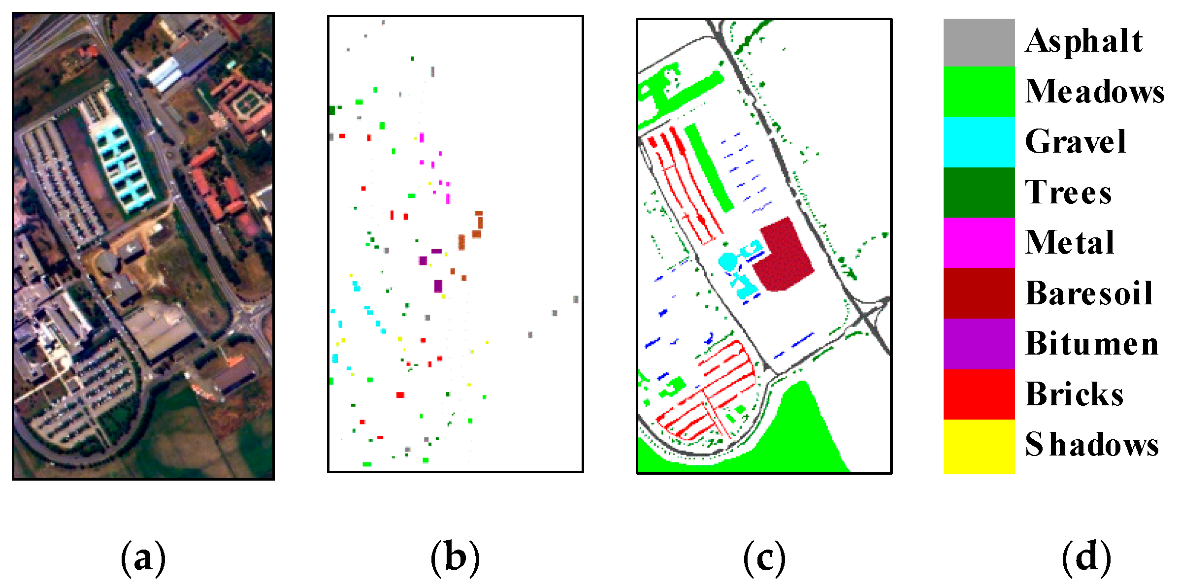
4.1.1. ROSIS Pavia University Data Set

ROSIS Pavia University hyperspectral images are acquired with a ROSIS optical sensor that provides 115 bands with spectral coverage ranging from 0.43 to 0.86 μm. The geometric resolution is 1.3 m. The image shown in Figure 1a was captured over the Engineering School, University of Pavia, Pavia, Italy. The image has 610 × 340 pixels with 103 spectral channels (a few original bands are very noisy and were discarded immediately after data acquisition). The validation data refer to nine land cover classes and are shown in Figure 1, with details about the number of samples given in

Table 2. Sample details for the ROSIS Pavia University hyperspectral image.

Class No.	Class	Test	Training
1	Asphalt	6631	548
2	Meadows	18,649	540
3	Gravel	2099	392
4	Trees	3064	524
5	Metal	1345	265
6	Bare soil	5029	532
7	Bitumen	1330	375
8	Bricks	3682	514
9	Shadows	947	231

.

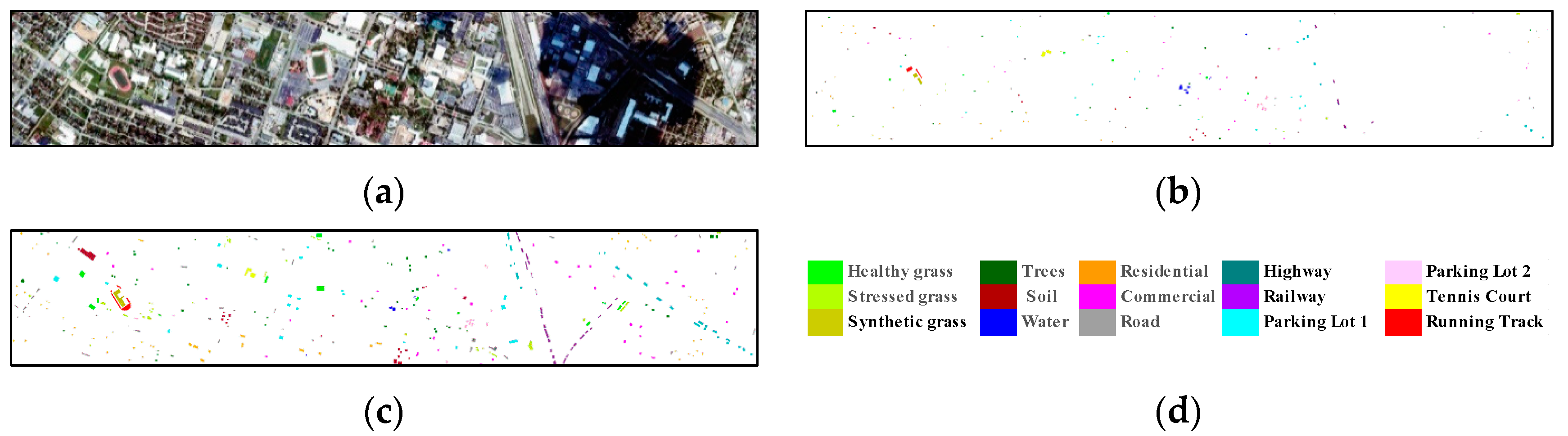
4.1.2. GRSS-DFC2013 Data Set

The second hyperspectral image was acquired at a spatial resolution of 2.5 m by the NSF-funded Center for Airborne Laser Mapping (NCALM) over the University of Houston campus and the neighboring urban area on 23 June 2012. The image has 349×1905 pixels with 144 spectral bands in the spectral range between 380 and 1050 nm. The 15 classes of interest selected by the Data Fusion Technical Committee (DFTC) of the IEEE Geoscience and Remote Sensing Society (GRSS) are shown in Figure 2 and reported in

Table 3. Sample details for the GRSS-DFC2013 hyperspectral image.

Class No.	Class	Training	Test	Class No.	Class	Training	Test
1	Healthy grass	198	1053	9	Road	193	1053
2	Stressed grass	190	1064	10	Highway	191	1036
3	Synthetic grass	192	505	11	Railway	181	1050
4	Trees	188	1056	12	Parking Lot 1	192	1041
5	Soil	186	1056	13	Parking Lot 2	184	285
6	Water	182	143	14	Tennis Court	181	247
7	Residential	196	1072	15	Running Track	187	473
8	Commercial	191	1046

with the corresponding numbers of samples for both the training and validation sets [50].

4.2. Experimental Setup

To evaluate the performance of XGBoost and the meta-XGBoost method proposed in this work, SVM, bagging, RaF, AdaBoost, MultiBoost, CVRFR, ExtraTrees and END-ERDT algorithms were adopted [6,9,10,11,44,51,52]. The critical parameters (e.g., minimum and maximum leaf sizes, maximum tree depth, tree pruning and smoothing rates, and tree size) of the DT-based EL classifiers were set by referring to the corresponding suggestions from the literature. The free parameters for the radial basis function (RBF) kernel-based SVM were tuned by 10-by-10 grid search optimization, with a search range of 0–1000 for gamma and 1–1000 for the cost factor.

To analyze the performance of the proposed spatial feature extractors, MPs, MPPRs, MSER_MPs, MSER_MPsM, EMPs and EMPPRs were applied to the two benchmark hyperspectral data sets presented previously [9,46,53,54]. To generate MPs and MPPR features from each data set, we applied a disk shape SE with n = 10 openings and closings based on conventional and partial reconstruction methods. The value of n was varied from one to ten with a step size of one. Thus, we will obtain a total of 2163 = 103 + 103 × 10 × 2 and 3024 = 144 + 144 × 10 × 2 dimensional data sets using the original spectral bands and a total of 70 = 10 + 3 × 10 × 2 and 67 = 7 + 3 × 10 × 2 dimensional data sets using the PCA-transformed features for ROSIS and GRSS-DFC2013, respectively. For fair comparison, we set the threshold =100 to 1000 with a step of 100 for selecting the objects in the MSER_MP and EMSER_MP feature extraction phases. Notably, MSER_MPsM and EMSER_MPsM, which contain extra mean pixel values within objects, will yield 3193 = 103 + 103 × 10 × 3, 4464 = 144 + 144 × 10 × 3, 100 = 10 + 3 × 10 × 3 and 97 = 7 + 3 × 10 × 3 dimensional data sets using the original spectral bands and PCA-transformed features for ROSIS and GRSS-DFC2013, respectively.

All the experiments were performed using R 3.5.0 software on a Windows 10 64-bit system run on an Intel Core™ i7-7820X CPU at 3.60 GHz and with 64 GB of RAM. The accuracy (OA), kappa statistic (k) and CPU run time for training were used to evaluate the classification performance of the all considered methods.

5. Analysis of Results and Discussion

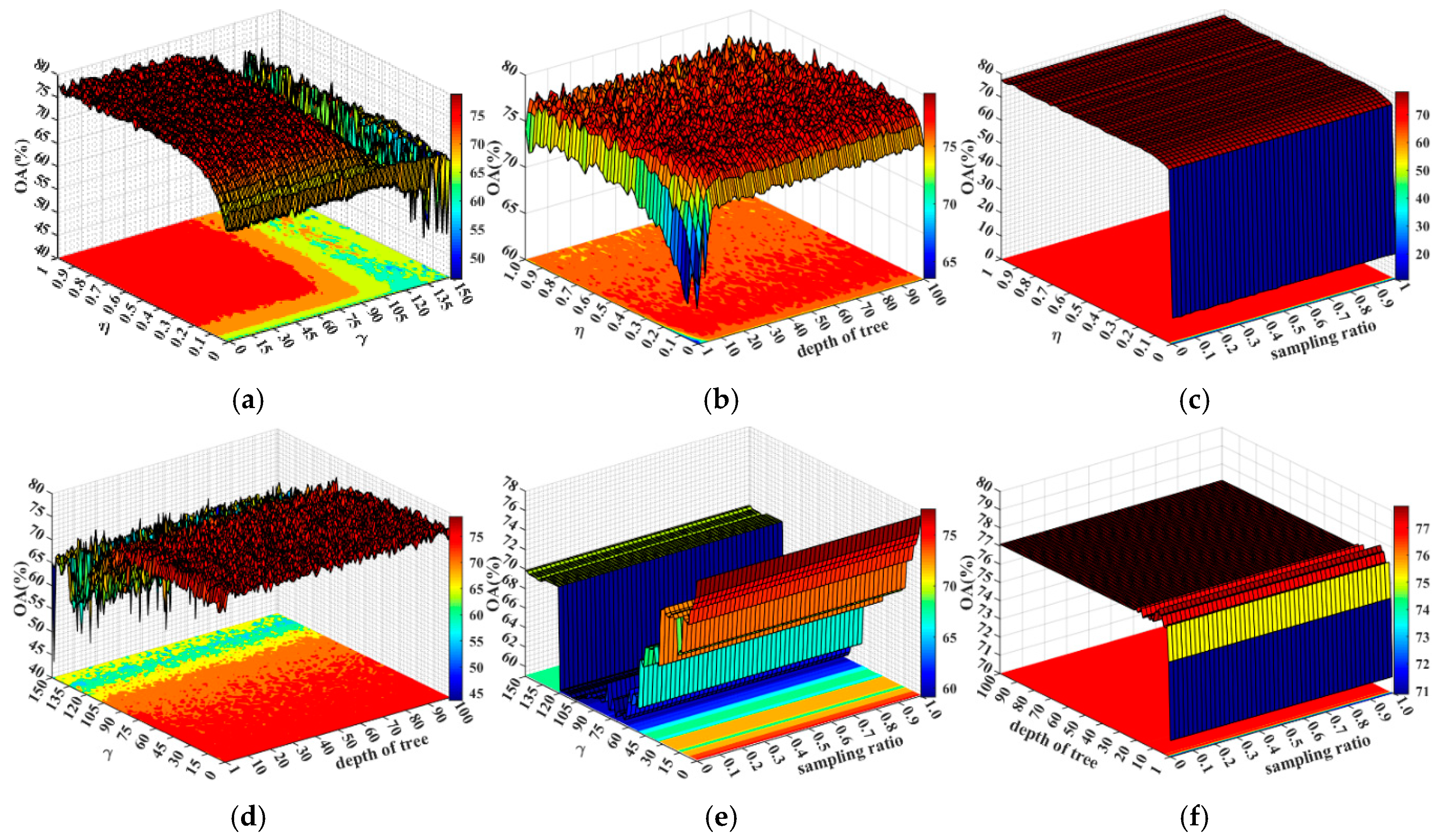
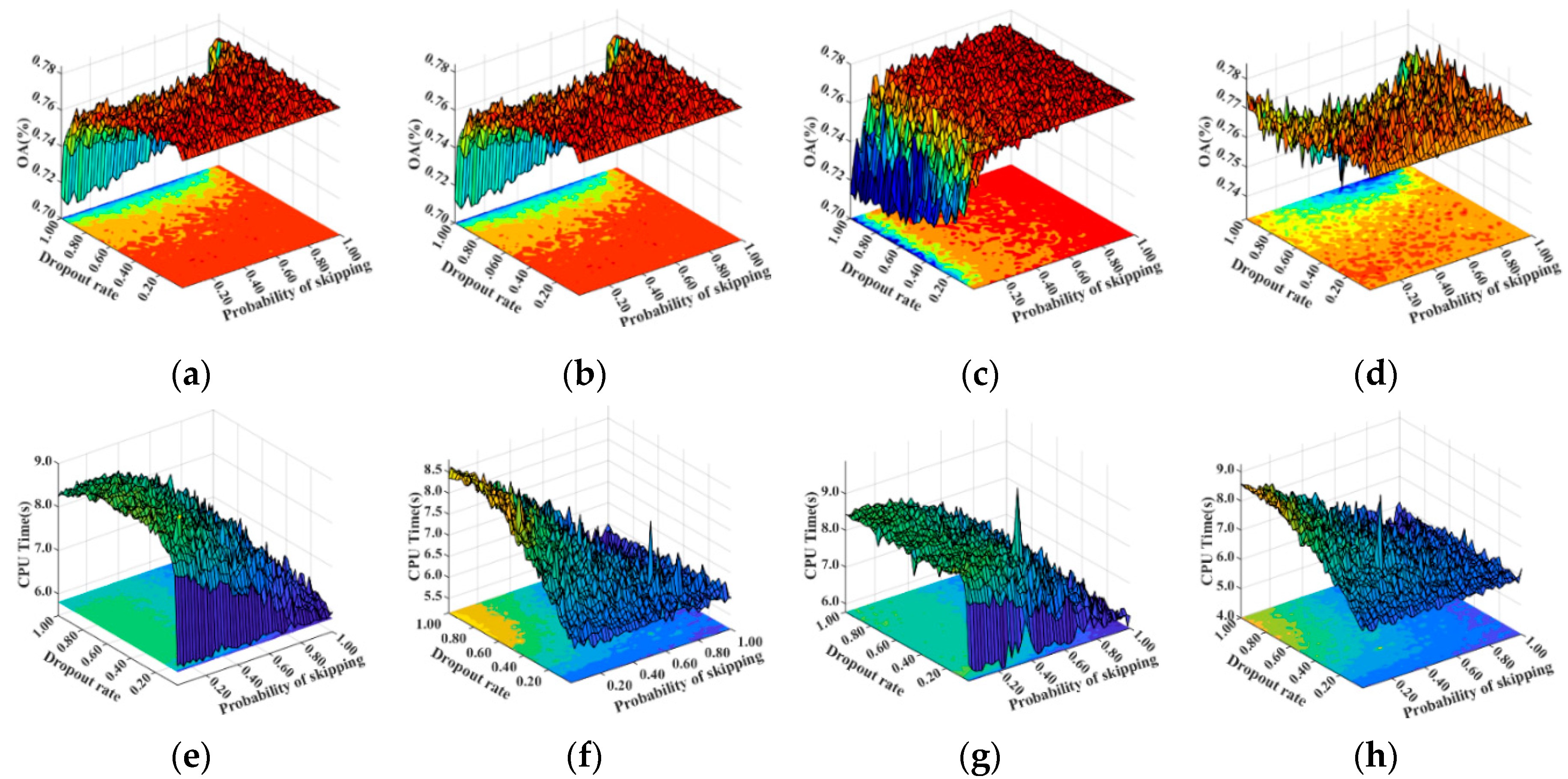
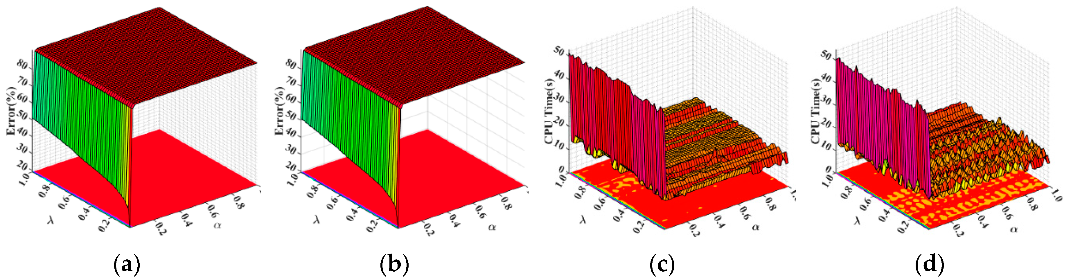
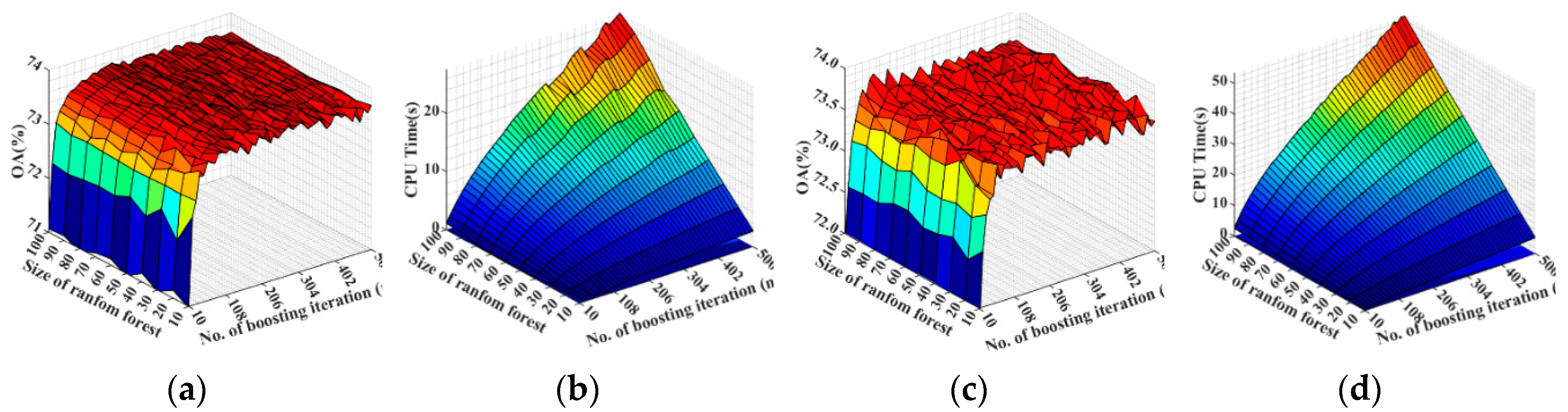
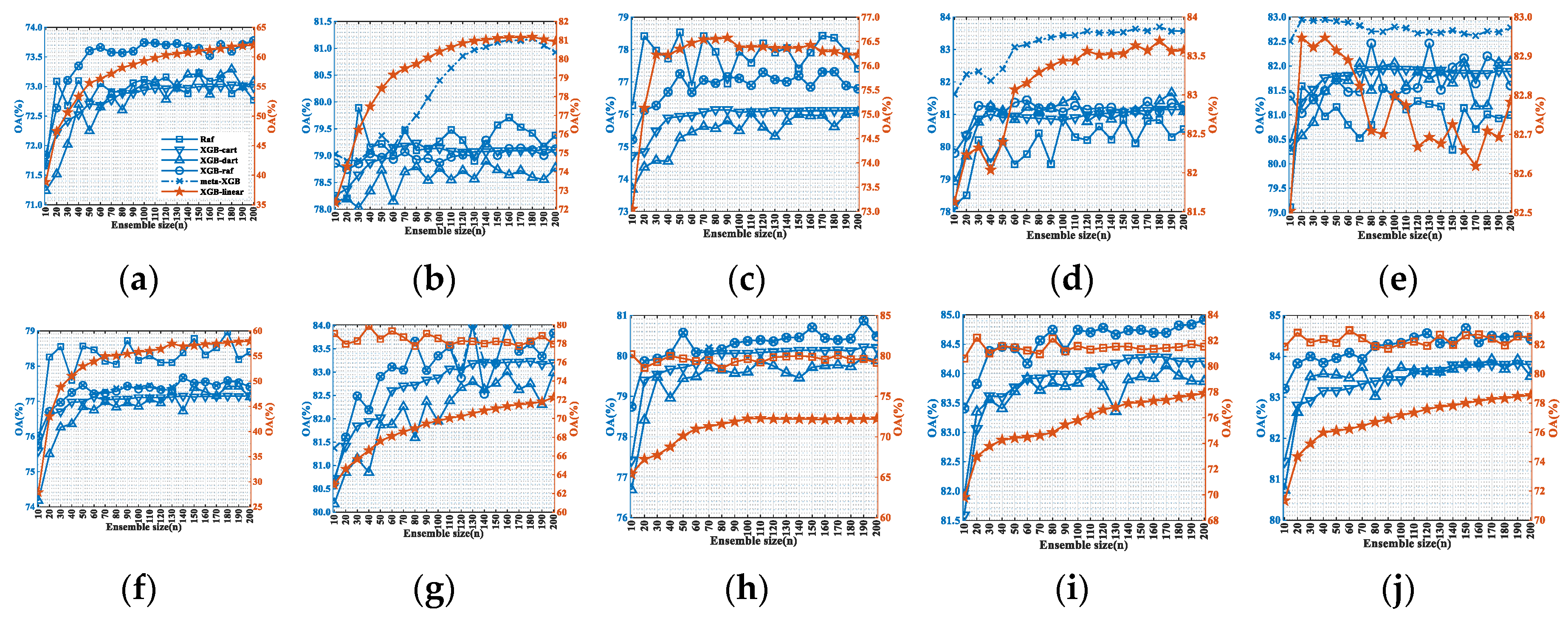
5.1. Parameter Configuration in XGBoost

XGBoost with the CART booster has more than 20 parameters, as mentioned above, but the learning rate ($\eta$,[0,1]), minimum split loss ($\gamma$,[0,$\infty$]), maximum tree depth ([0,$\infty$]) and subsample ratio of training samples ([0,1]) are the most important parameters [21,36,45]. Figure 3 illustrates the OA values versus the combination of these four parameters based on PCA10 features from the ROSIS University dataset. Notably, each OA surface graph was obtained by a combination of two parameters in a dynamic way, and the other two parameters were set by default, as suggested on the official website of XGBoost (https://xgboost.readthedocs.io/en/latest/parameter.html). First, according to the plots in the first row, the optimum range for the learning rate used to prevent overfitting is between 0.2 and 0.4. A large step size will shrink the feature weights to make the boosting process relatively conservative, and a small step size will not prevent overfitting. For the minimum split loss, a small value is always the best option, as shown in the plots in Figure 3a,d,e. In contrast, a large tree depth is always optimal for DTs to construct the best possible model. However, a large tree depth will make the model more complex and more likely to experience overfitting than would a small depth. Thus, an optimum range of between 5 and 10 for the maximum tree depth is recommended. In our next experiments, the maximum depth of trees was set to eight as the default for both efficiently training the low-complexity model and avoiding the potential overfitting issue. Additionally, according to the results for the sampling ratio parameter, there is no obvious impact on the classification accuracy. However, to prevent possible overfitting, especially in the limited sample training scenario, and maintain booster diversity in different boosting iterations, the optimum range for the sampling ratio should be between 0.5 and 1.

Figure 4 presents the OA and CPU time consumption in seconds versus the dropout rate ([0,1]; the fraction of the previous tree dropped during the dropout period) and probability of skipping the dropout procedure during a boosting iteration ([0,1]) for the DART booster, where different tree sampling algorithms (uniform and weighted) and normalization schemes (tree based: new trees have the same weights as dropped trees; forest based: new trees have the same weights as the sum of dropped trees) are combined in four ways. Notably, both the dropout rate and probability of skipping have significant impacts not only on the classification accuracy but also on the computational efficiency. Specifically, the probability of skipping does not have a significant influence on the classification accuracy with the parameter set for uniform sampling with both tree and forest normalization (see Figure 4a,b) but has a significant influence on the classification accuracy with the parameter set for weighted sampling with both tree and forest normalization (see Figure 4c,d). By comparing the results of uniform sampling versus weighted sampling and tree normalization versus forest normalization, it can be concluded that uniform sampling with tree or forest normalization is the best solution for building the model with optimal performance. For the dropout rate, a small value is always better than a large value, which is in accordance with the findings of previous works [21,36,46]. Additionally, a small dropout rate with a large probability of skipping is optimal for efficient model training. Therefore, dropout rate = 0.1 (set as 0, DART degradation to MART), probability of skipping = 0.5, and uniform sampling with tree normalization were used as defaults for XGBoost with the DART booster in subsequent experiments.

Figure 5 presents the critical parameters, including the ${\ell }_1$ and ${\ell }_2$ regularization terms $\alpha$ and $\lambda$, based on weighted and cyclic methods of shuffle feature selection and ordering for the linear booster. According to the plots in Figure 6, the ${\ell }_2$ regularization term $\lambda$ influences both the classification accuracy and training efficiency, and the optimum value is 0. There is no obvious influence on the classification accuracy or model training efficiency for the ${\ell }_1$ regularization term $\alpha$ with the cyclic method of shuffle feature selection and ordering.

Figure 6 illustrates the OA and CPU time consumption versus the number of trees and number of boosting iterations for XGBoost with the RaF booster based on raw features from the ROSIS University and DFC2013 datasets. Note that if early stopping is not adopted (which is the case in our experiments), the final model will consist of the number of trees in RaF multiplied by the number of boosting iterations. As shown in Figure 6, the number of boosting iterations has a greater influence on the classification accuracy than does the size of the RaF, and the computational complexity is increased by multiplying the size of the RaF by the number of boosting iterations. Moreover, values beyond approximately 100 boosting iterations do not improve the classification accuracy and are computationally expensive. Hence, the numbers of trees and boosting iterations were set to 10 and 100, respectively, for XGBoost with the RaF booster in subsequent experiments.

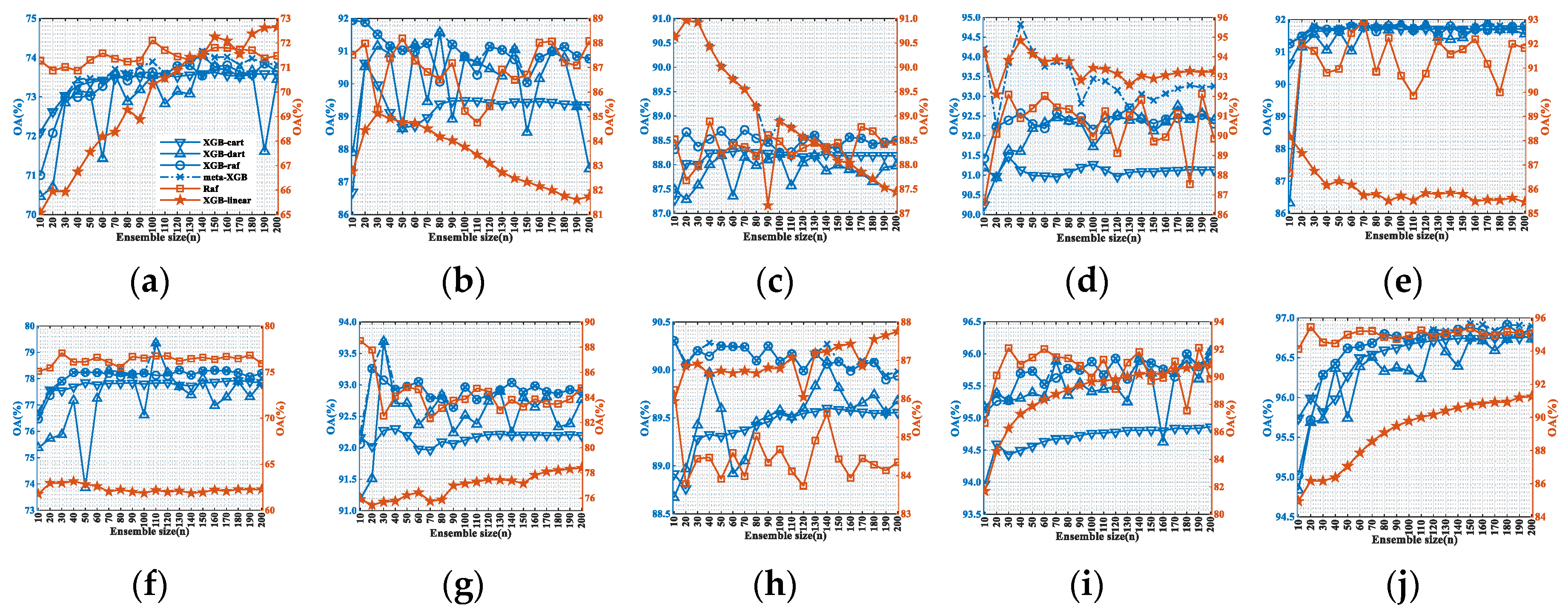
5.2. Classification Performance of Meta-XGBoost

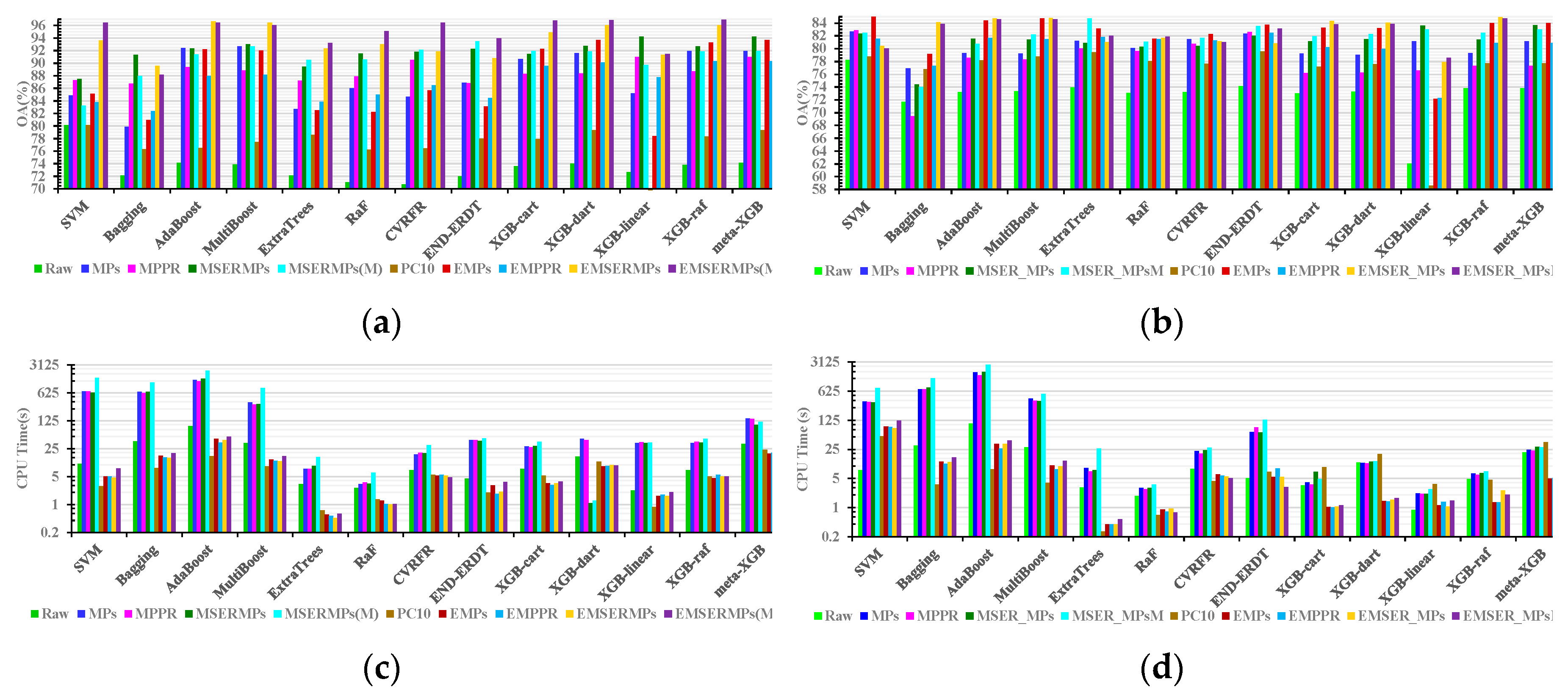
5.2.1. Classification Accuracy

In Figure 7 and Figure 8, we present the results of OA from the considered classifiers with increasing ensemble size for various features from the ROSIS University and DFC2013 hyperspectral data sets, respectively. Each point on the x-axis represents the size of trees in a conventional RaF and the number of boosting iterations for meta-XGBoost and XGBoost with the CART, DART, linear and RaF boosters. The left y-axis represents the overall classification accuracies of meta-XGBoost and XGBoost with the CART, DART and RaF boosters, and the right y-axis represents the overall classification accuracies of the conventional RaF and XGBoost combined method with a linear booster (Figure 7) or only XGBoost with a linear booster (Figure 8). Notably, the XGBoost with a linear booster classifier and conventional RaF classifier displayed large variations in classification accuracy, in contrast with the results of meta-XGBoost and XGBoost with the CART, DART and RaF boosters. If there were only one y-axis, it would be difficult to visually analyze the differences among the meta-XGBoost and XGBoost methods with the CART, DART and RaF boosters, which display small variations in classification accuracy. Figure 9 presents the OA and CPU time consumption in seconds for the considered classifiers and all the features from the ROSIS University and DFC2013 hyperspectral data sets.

From the results shown in Figure 7, Figure 8 and Figure 9, differences in the classification accuracy of XGBoost with the CART, DART, linear and RaF boosters are clear for the different datasets and for features from the same dataset, as expected. For instance, XGBoost with the linear booster exhibited the highest OA values for MPPR features extracted from the raw bands of the ROSIS University data at small numbers of boosting iterations (see Figure 7c) but yielded the worst OA values for PC10 features, with no positive or negative influences based on the number of boosting iterations (see Figure 7f). When comparing the results of XGBoost with the CART, DART and RaF boosters, XGBoost with the RaF booster is more stable than XGBoost with the CART and DART boosters in most cases and generally displays better performance, as illustrated by the blue lines with circle markers. This result is reasonable because both theoretically and practically, the RaF ensemble classifier is stronger than the single CART and DART classifiers. Other studies have found that the DART booster is superior to the CART booster and that XGBoost is superior to the conventional RaF classifier; these findings were not consistently observed in our experiments. In contrast, XGBoost with the DART booster display larger variations in OA values than XGBoost with the CART booster, as illustrated by the blue lines with upward-pointing triangles in Figure 7a–j and Figure 8a,f–h. Notably, the dropout technique introduced in the DART booster can overcome the overfitting issue of CART, and it might also introduce instability, especially for scenarios with large numbers of boosting iterations. According to the theorem of EL, if diversities exist among classifiers that yield better performance than random guessing, improvements can always be achieved with an ensemble system. By comparing the OA results of the proposed meta-XGBoost method with those of XGBoost with the CART, DART, linear and RaF boosters, higher and more stable results can be observed for meta-XGBoost in almost all cases, as shown by the blue dotted lines with cross markers in Figure 7 and Figure 8. A comparison of the OA bars in Figure 9a,b suggests that better results can be obtained with meta-XGBoost than with the SVM, AdaBoost, MultiBoost, RaF, ExtraTree, END-ERDT and CVRFR classifiers based on both experimental datasets; this finding is supported by the results in

Table 4. OA and kappa values of the considered classifiers for various features from the ROSIS University data.

Features	Raw		MPs		MPPR		MSERMPs		MSERMPs(M)		PC10		EMPs		EMPPR		EMSERMPs		EMSERMPs(M)
Metrics	OA	k	OA	k	OA	k	OA	k	OA	k	OA	k	OA	k	OA	k	OA	k	OA	k
SVM	80.18	0.75	84.86	0.81	87.25	0.83	87.50	0.84	83.29	0.79	80.16	0.75	85.15	0.81	83.79	0.79	93.62	0.92	86.72	0.83
Bagging	72.18	0.66	79.90	0.74	86.74	0.82	91.32	0.88	87.96	0.84	76.36	0.70	80.97	0.76	82.42	0.77	89.59	0.87	88.15	0.85
AdaBoost	74.18	0.68	92.44	0.90	89.38	0.86	92.34	0.90	91.41	0.89	76.51	0.71	92.21	0.89	87.93	0.84	96.63	0.96	96.46	0.95
MultiBoost	73.91	0.68	92.66	0.90	88.80	0.85	93.03	0.91	92.71	0.90	77.49	0.72	92.01	0.89	88.18	0.84	96.44	0.95	96.04	0.95
ExtraTrees	72.18	0.66	82.69	0.78	87.22	0.83	89.41	0.86	90.53	0.88	78.63	0.73	82.53	0.78	83.84	0.79	92.33	0.90	93.22	0.91
RaF	71.08	0.64	85.99	0.82	87.85	0.84	91.54	0.89	90.56	0.88	76.29	0.70	82.29	0.77	84.99	0.80	93.02	0.91	95.06	0.94
CVRFR	70.73	0.64	84.70	0.80	90.50	0.87	91.78	0.89	92.16	0.89	76.48	0.71	85.71	0.82	86.49	0.82	91.88	0.90	96.43	0.95
END-ERDT	72.01	0.66	86.88	0.83	86.77	0.84	92.29	0.90	93.46	0.91	78.03	0.73	83.15	0.79	84.46	0.80	90.78	0.88	93.91	0.92
XGB-CART	73.63	0.68	90.63	0.87	88.30	0.84	91.47	0.89	91.89	0.89	77.93	0.72	92.28	0.90	89.60	0.86	94.86	0.93	96.77	0.96
XGB-DART	74.06	0.68	91.57	0.89	88.39	0.84	92.75	0.90	91.85	0.89	79.34	0.74	93.69	0.92	90.08	0.86	96.04	0.95	96.85	0.96
XGB-linear	72.65	0.66	85.19	0.81	90.96	0.88	94.21	0.92	89.70	0.86	63.16	0.55	78.39	0.73	87.75	0.84	91.35	0.89	91.49	0.89
XGB-RaF	73.85	0.68	91.95	0.90	88.71	0.85	92.70	0.90	91.84	0.89	78.33	0.73	93.26	0.91	90.31	0.87	96.00	0.95	96.91	0.97
meta-XGB	74.17	0.68	91.95	0.90	90.96	0.88	94.21	0.92	91.94	0.89	79.34	0.74	93.69	0.92	90.31	0.87	96.04	0.95	96.93	0.97

and

Table 5. OA and kappa values of the considered classifiers for various features from the DFC2013 data.

Features	Raw		MPs		MPPR		MSER_MPs		MSER_MPsM		PC10		EMPs		EMPPR		EMSER_MPs		EMSER_MPsM
Metrics	OA	k	OA	k	OA	k	OA	k	OA	k	OA	k	OA	k	OA	k	OA	k	OA	k
SVM	78.27	0.77	82.70	0.81	82.85	0.81	82.32	0.81	82.49	0.81	78.78	0.77	85.07	0.84	81.53	0.80	80.44	0.79	80.01	0.78
Bagging	71.72	0.71	76.95	0.75	69.49	0.67	74.43	0.72	73.97	0.72	76.79	0.75	79.18	0.78	77.31	0.75	84.14	0.83	83.89	0.83
AdaBoost	73.23	0.71	79.33	0.78	78.58	0.77	81.56	0.80	80.75	0.79	78.20	0.76	84.38	0.83	81.71	0.80	84.72	0.83	84.55	0.83
MultiBoost	73.35	0.71	79.21	0.78	78.34	0.77	81.44	0.80	82.21	0.81	78.76	0.77	84.72	0.83	81.49	0.80	84.78	0.83	84.55	0.83
ExtraTrees	73.89	0.72	81.22	0.80	80.02	0.78	80.84	0.79	84.74	0.83	79.45	0.78	83.14	0.82	81.81	0.80	80.98	0.79	82.02	0.81
RaF	73.12	0.71	80.09	0.78	79.59	0.78	80.26	0.79	81.07	0.80	78.07	0.76	81.56	0.80	81.50	0.80	81.66	0.80	81.84	0.80
CVRFR	73.24	0.71	81.46	0.80	80.72	0.79	80.40	0.79	81.67	0.80	77.65	0.76	82.27	0.81	81.26	0.80	81.12	0.80	80.99	0.80
END-ERDT	74.10	0.72	82.32	0.81	82.59	0.81	81.98	0.81	83.51	0.82	79.52	0.78	83.72	0.82	82.46	0.81	80.77	0.79	83.10	0.82
XGB-CART	73.03	0.71	79.24	0.78	76.14	0.74	81.16	0.80	81.93	0.80	77.16	0.75	83.23	0.82	80.22	0.79	84.28	0.83	83.81	0.83
XGB-DART	73.29	0.71	79.01	0.77	76.27	0.74	81.49	0.80	82.30	0.81	77.59	0.76	83.17	0.82	79.97	0.78	84.05	0.83	83.88	0.83
XGB-linear	62.10	0.59	81.17	0.80	76.57	0.75	83.58	0.82	82.97	0.82	58.63	0.55	72.17	0.70	72.32	0.70	77.90	0.76	78.56	0.77
XGB-RaF	73.78	0.72	79.29	0.77	77.32	0.75	81.44	0.80	82.46	0.81	77.67	0.76	84.01	0.82	80.89	0.79	84.92	0.84	84.69	0.84
meta-XGB	73.78	0.72	81.19	0.80	77.67	0.75	83.69	0.82	82.95	0.81	77.67	0.76	84.01	0.82	80.89	0.79	84.92	0.84	84.69	0.84

. Specifically, this finding is evident in cases that use advanced spectral-spatial features, including the MP, MPPR, MSER_MP, MSER_MPsM methods and their extended versions. Accordingly, the XGBoost classifier can be boosted further by using an ensemble of four boosters.

5.2.2. Computational Efficiency

Computational efficiency is considered a key factor when evaluating classifier performance. In accordance with the plots in Figure 9a,b, which show the classification accuracies, the plots in Figure 9c,d show the CPU time in seconds for the training phase with the considered classifiers and using all the considered features. Because the free parameters of all the ensemble classifiers were set as constants before model training, the CPU time consumption for the 10-by-10 grid search optimization procedure was not included for the SVM for fair comparison. The numbers of trees in the bagging, RaF, ExtraTree, CVRFR, and END-ERDT methods and boosting iterations in AdaBoost, MultiBoost, and XGBoost with the CART, DART and linear boosters and meta-XGBoost are set to 100 by default; additionally, the number of parallel trees in XGBoost with the RaF booster was set to 10.

When considering the influence of data dimensionality, high-data dimensionality always increases the model training inefficiency, especially for the SVM, bagging, AdaBoost, and MultiBoost methods. In contrast, based on the bar plots for classifiers based on all the considered features, ExtraTrees yields the fastest model training efficiency for low-dimensionality data. The bar plots for the features of PC10 and spatial features extracted from the first three principal components also reflect this trend. This result is in accordance with the findings of our previous works [9,11]. As a highly efficient and scalable algorithm, XGB-boost with the CART, DART and linear boosters is much more efficient (at least five times faster) than the SVM, AdaBoost and MultiBoost methods and less efficient than the conventional RaF and ExtraTrees classifiers, especially in the case of datasets with high dimensionality. Combined with the results from the previous subsection, meta-XGBoost can be an alternative to state-of-the-art classifiers, including RBF kernel-based SVMs, AdaBoost and MultiBoost, based on the generalized classification accuracy and computational efficiency in model training, especially for data with high dimensionality, such as hyperspectral imagery.

5.3. Performance of EMSER_MPs

In our previous work, the superiority of MSER_MPs over the conventional MP and MPPR methods was verified for VHR remote sensing images over urban areas based on both visual interpretation and classification [9]. Here, we analyze the performance of the EMSER_MPs from the aspect of classification accuracy. According to the results shown in Figure 7, Figure 8 and Figure 9, the OA values of MSER_MPs and MSER_MPsM are higher than the OA values of the raw, MP and MPPR feature methods. This result was also observed for EMSER_MPs and EMSER_MPsM in all experiments with the considered datasets. For instance, classifiers including meta-XGBoost, XGBoost with the RaF booster and RaF yielded classification accuracies higher than 95% on average with EMSER_MPs and EMSER_MPsM features from the ROSIS University data; additionally, the maximum classification accuracy was 93.69% for meta-XGBoost and XGBoost with the DART booster and 90.31% for meta-XGBoost and XGBoost with the RaF booster based on EMPs and EMPPR features (see the results in Figure 7 and Figure 9a, and Table 4). Similarly, the classification performance of EMSER_MPs and EMSER_MPsM was superior to that of EMPs and EMPPR, as can be observed in Figure 8 and Figure 9b and Table 4 based on experiments with the DFC2013 data set. For example, the highest classification accuracy (OA = 85.07) was reached by the SVM using EMP features, but the second-best value (OA = 84.92%) was obtained with the proposed meta-XGBoost method using EMSER_MP features. If we compare the results from all other classifiers using EMSESR_MP and EMSER_MPsM features, as shown in Figure 10 by the bars in magenta and orange colors and in the last two columns of Table 4, the classification accuracies reached by using these two feature sets are generally higher than others in most cases. Thus, we can conclude that the proposed EMSER_MP approach can be an alternative to state-of-the-art spatial feature extractors, including MPs, EMPs, MPPR, EMPPR and MSER_MPs, for hyperspectral image classification.

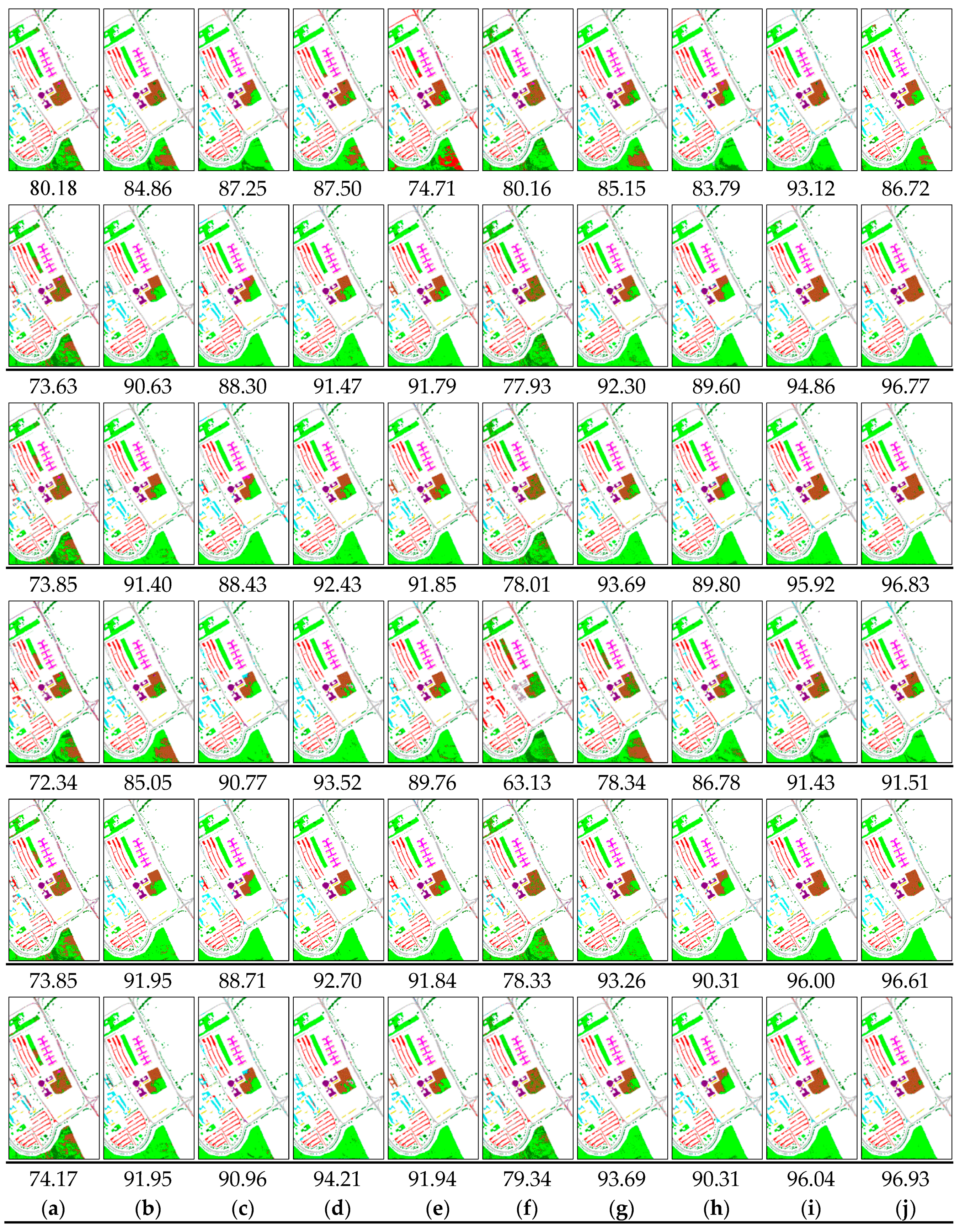
5.4. Classification Maps

Finally, in Figure 10, we present the classification maps with OA values for the classifiers, including SVM; XGBoost with the CART, DART and linear boosters; and meta-XGBoost, using various features from the ROSIS University data set. In addition, Figure 11 shows the classification maps with OA values for the SVM and proposed meta-XGBoost methods using all the considered features from the second experimental data set. Due to space limitations, and for clear visualization, we only selected the results from several methods to show in Figure 10 and Figure 11; moreover, Table 4 and Table 5 show the overall classification accuracies with kappa coefficient values for all classifiers using all the considered features.

6. Conclusions

According to the literature, XGBoost has shown remarkable performance in some classification, regression and ranking tasks. However, the use of XGBoost has not been extensively investigated in the remote sensing image classification context with spectral and spectral-spatial features. Additionally, several issues of potential overfitting, reduced training efficiency, decreased predictive performance, unstable early stopping, and being limited to solving nonlinearly separable problems remain for XGBoost with different boosters in practical applications. In this regard, a novel version of XGBoost, meta-XGBoost, was proposed to overcome the above issues.

According to the results, the following conclusions can be drawn. First, the proposed EMSER_MP features are better than all the MP, MPPR, MSER_MP, EMP and EMPPR features. Furthermore, some previous findings suggested that XGBoost with a DART booster is superior to XGBoost with a CART booster and that XGBoost is superior to conventional RaF methods in the spectral-spatial classification of hyperspectral images. However, the classification accuracy of SVM, AdaBoost, MultiBoost, ExtraTrees and END-ERDT classifiers was better than that of XGBoost with the CART, DART, linear and RaF boosters in some cases. Additionally, XGBoost with the RaF booster yielded a higher classification accuracy than XGBoost with the CART booster, but the best results were consistently obtained by meta-XGBoost, especially when advanced features were used. Finally, based on both the generalized classification accuracy and computational efficiency of model training, the proposed meta-XGBoost classifier could be an alternative to state-of-the-art classifier, including RBF kernel-based SVM, AdaBoost and MultiBoost classifiers, especially for high-dimension and nonlinearly separable data such as hyperspectral imagery used in spectral-spatial classification.

References

1. Hughes, G. On the mean accuracy of statistical pattern recognizers. IEEE Trans. Inf. Theory 1968, 14, 55–63. [Google Scholar] [CrossRef] [Green Version]
2. Gamba, P.; Dell’Acqua, F.; Stasolla, M.; Trianni, G.; Lisini, G. Limits and challenges of optical high-resolution satellite remote sensing for urban applications. In Urban Remote Sensing—Monitoring, Synthesis and Modelling in the Urban Environment; Yang, X., Ed.; Wiley: New York, NY, USA, 2011; pp. 35–48. [Google Scholar]
3. Fauvel, M.; Tarabalka, Y.; Benediktsson, J.A.; Chanussot, J.; Tilton, J.C. Advances in spectral-spatial classification of hyperspectral images. Proc. IEEE 2013, 101, 652–675. [Google Scholar] [CrossRef] [Green Version]
4. Plaza, A.; Benediktsson, J.A.; Boardman, J.W.; Brazile, J.; Bruzzone, L.; Camps-Valls, G.; Chanussot, J.; Fauvel, M.; Gamba, P.; Gualtieri, A.; et al. Recent advances in techniques for hyperspectral image processing. Remote Sens. Environ. 2009, 113, S110–S122. [Google Scholar] [CrossRef]
5. Melgani, F.; Bruzzone, L. Classification of hyperspectral remote sensing images with support vector machines. IEEE Trans. Geosci. Remote Sens. 2004, 42, 1778–1790. [Google Scholar] [CrossRef] [Green Version]
6. Mountrakis, G.; Im, J.; Ogole, C. Support vector machines in remote sensing: A review. ISPRS J. Photogramm. Remote Sens. 2011, 66, 247–259. [Google Scholar] [CrossRef]
7. Du, P.; Samat, A.; Waske, B.; Liu, S.; Li, Z. Random forest and rotation forest for fully polarized SAR image classification using polarimetric and spatial features. ISPRS J. Photogramm. Remote Sens. 2015, 105, 38–53. [Google Scholar] [CrossRef]
8. Samat, A.; Du, P.; Liu, S.; Li, J.; Cheng, L. E2LMs: Ensemble Extreme Learning Machines for Hyperspectral Image Classification. IEEE J. Sel. Top. Appl. Earth Obs. Remote Sens. 2014, 7, 1060–1069. [Google Scholar] [CrossRef]
9. Samat, A.; Persello, C.; Liu, S.; Li, E.; Miao, Z.; Abuduwaili, J. Classification of VHR multispectral images using extratrees and maximally stable extremal region-guided morphological profile. IEEE J. Sel. Top. Appl. Earth Obs. Remote Sens. 2018, 11, 3179–3195. [Google Scholar] [CrossRef]
10. Samat, A.; Gamba, P.; Liu, S.; Miao, Z.; Li, E.; Abuduwaili, J. Quad-PolSAR data classification using modified random forest algorithms to map halophytic plants in arid areas. Int. J. Appl. Earth Obs. Geoinf. 2018, 73, 503–521. [Google Scholar] [CrossRef]
11. Samat, A.; Yokoya, N.; Du, P.; Liu, S.; Ma, L.; Ge, Y.; Lin, C. Direct, ECOC, ND and END Frameworks—Which One Is the Best? An Empirical Study of Sentinel-2A MSIL1C Image Classification for Arid-Land Vegetation Mapping in the Ili River Delta, Kazakhstan. Remote Sens. 2019, 11, 1953. [Google Scholar] [CrossRef] [Green Version]
12. Samat, A.; Li, J.; Liu, S.; Du, P.; Miao, Z.; Luo, J. Improved hyperspectral image classification by active learning using pre-designed mixed pixels. Pattern Recognit. 2016, 51, 43–58. [Google Scholar] [CrossRef]
13. Du, P.; Bai, X.; Tan, K.; Xue, Z.; Samat, A.; Xia Ju Li, E.; Su, H.; Liu, W. Advances of Four Machine Learning Methods for Spatial Data Handling: A Review. J. Geovisualization Spat. Anal. 2020, 4, 13. [Google Scholar] [CrossRef]
14. Ham, J.; Chen, Y.; Crawford, M.M.; Ghosh, J. Investigation of the random forest framework for classification of hyperspectral data. IEEE Trans. Geosci. Remote Sens. 2005, 43, 492–501. [Google Scholar] [CrossRef] [Green Version]
15. Belgiu, M.; Drăguţ, L. Random forest in remote sensing: A review of applications and future directions. ISPRS J. Photogramm. Remote Sens. 2016, 114, 24–31. [Google Scholar] [CrossRef]
16. Chan, J.C.W.; Paelinckx, D. Evaluation of Random Forest and Adaboost tree-based ensemble classification and spectral band selection for ecotope mapping using airborne hyperspectral imagery. Remote Sens. Environ. 2008, 112, 2999–3011. [Google Scholar] [CrossRef]
17. Johnson, R.; Zhang, T. Learning nonlinear functions using regularized greedy forest. IEEE Trans. Pattern Anal. Mach. Intell. 2014, 36, 942–954. [Google Scholar] [CrossRef] [Green Version]
18. Friedman, J.H. Greedy function approximation: A gradient boosting machine. Ann. Stat. 2001, 29, 1189–1232. [Google Scholar] [CrossRef]
19. Ye, J.; Chow, J.H.; Chen, J.; Zheng, Z. Stochastic gradient boosted distributed decision trees. In Proceedings of the 18th ACM Conference on INFORMATION and Knowledge management, Hongkong, China, 2–6 November 2009; pp. 2061–2064. [Google Scholar]
20. Ma, X.; Ding, C.; Luan, S.; Wang, Y.; Wang, Y. Prioritizing influential factors for freeway incident clearance time prediction using the gradient boosting decision trees method. IEEE Trans. Intell. Transp. Syst. 2017, 18, 2303–2310. [Google Scholar] [CrossRef]
21. Chen, T.; Guestrin, C. Xgboost: A scalable tree boosting system. In Proceedings of the 22nd Acm Sigkdd International Conference on Knowledge Discovery and Data Mining, San Francisco, CA, USA, 13–17 August 2016; pp. 785–794. [Google Scholar]
22. Natekin, A.; Knoll, A. Gradient boosting machines, a tutorial. Front. Neurorobot. 2013, 7, 21. [Google Scholar] [CrossRef] [Green Version]
23. Zheng, Z.; Zha, H.; Zhang, T.; Chapelle, O.; Chen, K.; Sun, G. A general boosting method and its application to learning ranking functions for web search. In Proceedings of the Advances in Neural Information Processing Systems, Vancouver, BC, Canada, 12 December 2008; pp. 1697–1704. [Google Scholar]
24. Lombardo, L.; Cama, M.; Conoscenti, C.; Märker, M.; Rotigliano, E. Binary logistic regression versus stochastic gradient boosted decision trees in assessing landslide susceptibility for multiple-occurring landslide events: Application to the 2009 storm event in Messina (Sicily, southern Italy). Nat. Hazards 2015, 79, 1621–1648. [Google Scholar] [CrossRef]
25. Lin, L.; Yue, W.; Mao, Y. Multi-class image classification based on fast stochastic gradient boosting. Informatica 2014, 38, 145–153. [Google Scholar]
26. Guelman, L. Gradient boosting trees for auto insurance loss cost modeling and prediction. Expert Syst. Appl. 2012, 39, 3659–3667. [Google Scholar] [CrossRef]
27. Friedman, J.H. Stochastic gradient boosting. Comput. Stat. Data Anal. 2002, 38, 367–378. [Google Scholar] [CrossRef]
28. Lawrence, R.; Bunn, A.; Powell, S.; Zambon, M. Classification of remotely sensed imagery using stochastic gradient boosting as a refinement of classification tree analysis. Remote Sens. Environ. 2004, 90, 331–336. [Google Scholar] [CrossRef]
29. Moisen, G.G.; Freeman, E.A.; Blackard, J.A.; Frescino, T.S.; Zimmermann, N.E.; Edwards, T.C. Predicting tree species presence and basal area in Utah: A comparison of stochastic gradient boosting, generalized additive models, and tree-based methods. Ecol. Model. 2006, 199, 176–187. [Google Scholar] [CrossRef]
30. Chirici, G.; Scotti, R.; Montaghi, A.; Barbati, A.; Cartisano, R.; Lopez, G.; Marchetti, M.; McRoberts, R.E.; Olsson, H.; Corona, P. Stochastic gradient boosting classification trees for forest fuel types mapping through airborne laser scanning and IRS LISS-III imagery. Int. J. Appl. Earth Obs. Geoinf. 2013, 25, 87–97. [Google Scholar] [CrossRef] [Green Version]
31. Freeman, E.A.; Moisen, G.G.; Coulston, J.W.; Wilson, B.T. Random forests and stochastic gradient boosting for predicting tree canopy cover: Comparing tuning processes and model performance. Can. J. For. Res. 2015, 46, 323–339. [Google Scholar] [CrossRef] [Green Version]
32. Panda, B.; Herbach, J.S.; Basu, S.; Bayardo, R.J. Planet: Massively parallel learning of tree ensembles with mapreduce. Proc. Vldb Endow. 2009, 2, 1426–1437. [Google Scholar] [CrossRef]
33. Meng, Q.; Ke, G.; Wang, T.; Chen, W.; Ye, Q.; Ma, Z.M.; Liu, T. A communication-efficient parallel algorithm for decision tree. In Proceedings of the Advances in Neural Information Processing Systems, Barcelona, Spain, 5–10 December 2016; pp. 1279–1287. [Google Scholar]
34. Chen, J.; Li, K.; Tang, Z.; Bilal, K.; Yu, S.; Weng, C.; Li, K. A parallel random forest algorithm for big data in a spark cloud computing environment. IEEE Trans. Parallel Distrib. Syst. 2016, 28, 919–933. [Google Scholar] [CrossRef] [Green Version]
35. Abuzaid, F.; Bradley, J.K.; Liang, F.T.; Feng, A.; Yang, L.; Zaharia, M.; Talwalkar, A.S. Yggdrasil: An Optimized System for Training Deep Decision Trees at Scale. In Proceedings of the Advances in Neural Information Processing Systems, Barcelona, Spain, 5–10 December 2016; pp. 3817–3825. [Google Scholar]
36. Zhang, H.; Si, S.; Hsieh, C.J. GPU-acceleration for Large-scale Tree Boosting. arXiv 2017, arXiv:1706.08359. [Google Scholar]
37. Dong, H.; Xu, X.; Wang, L.; Pu, F. Gaofen-3 PolSAR image classification via XGBoost and polarimetric spatial information. Sensors 2018, 18, 611. [Google Scholar] [CrossRef] [Green Version]
38. Yu, S.; Chen, Z.; Yu, B.; Wang, L.; Wu, B.; Wu, J.; Zhao, F. Exploring the relationship between 2D/3D landscape pattern and land surface temperature based on explainable eXtreme Gradient Boosting tree: A case study of Shanghai, China. Sci. Total Environ. 2020, 725, 1–15. [Google Scholar] [CrossRef] [PubMed]
39. Zhang, H.; Eziz, A.; Xiao, J.; Tao, S.; Wang, S.; Tang, Z.; Fang, J. High-Resolution Vegetation Mapping Using eXtreme Gradient Boosting Based on Extensive Features. Remote Sens. 2019, 11, 1505. [Google Scholar] [CrossRef] [Green Version]
40. Chen, Z.; Zhang, T.; Zhang, R.; Zhu, Z.; Yang, J.; Chen, P.; Ou, C.; Guo, Y. Extreme gradient boosting model to estimate PM2.5 concentrations with missing filled satellite data in China. Atmos. Environ. 2019, 202, 180–189. [Google Scholar] [CrossRef]
41. Freund, Y. An adaptive version of the boost by majority algorithm. Mach. Learn. 2001, 43, 293–318. [Google Scholar] [CrossRef]
42. Rashmi, K.V.; Gilad-Bachrach, R. DART: Dropouts meet Multiple Additive Regression Trees. In Proceedings of the International Conference on Artificial Intelligence and Statistics (AISTATS), San Diego, CA, USA, 9–12 May 2015; pp. 489–497. [Google Scholar]
43. Bradley, J.K.; Kyrola, A.; Bickson, D.; Guestrin, C. Parallel coordinate descent for l1-regularized loss minimization. arXiv 2011, arXiv:1105.5379. [Google Scholar]
44. Breiman, L. Random forests. Mach. Learn. 2001, 45, 5–32. [Google Scholar] [CrossRef] [Green Version]
45. Chen, T.; He, T.; Benesty, M. xgboost: Extreme Gradient Boosting; R Package Version 0.3-0; Technical Report; R Foundation for Statistical Computing: Vienna, Austria.
46. Benediktsson, J.A.; Palmason, J.A.; Sveinsson, J.R. Classification of hyperspectral data from urban areas based on extended morphological profiles. IEEE Trans. Geosci. Remote Sens. 2005, 43, 480–491. [Google Scholar] [CrossRef]
47. Donoser, M.; Bischof, H. Efficient maximally stable extremal region (MSER) tracking. In Proceedings of the 2006 IEEE Computer Society Conference on Computer Vision and Pattern Recognition (CVPR’06), New York, NY, USA, 17–22 June 2006; Volume 1, pp. 553–560. [Google Scholar]
48. Forssén, P.E. Maximally stable colour regions for recognition and matching. In Proceedings of the 2007 IEEE Conference on Computer Vision and Pattern Recognition, Minneapolis, MN, USA, 17–22 June 2007; pp. 1–8. [Google Scholar]
49. Mitchell, R.; Frank, E. Accelerating the XGBoost algorithm using GPU computing. Peerj Comput. Sci. 2017, 3, e127. [Google Scholar] [CrossRef]
50. Debes, C.; Merentitis, A.; Heremans, R.; Hahn, J.; Frangiadakis, N.; van Kasteren, T.; Philips, W. Hyperspectral and LiDAR data fusion: Outcome of the 2013 GRSS data fusion contest. IEEE J. Sel. Top. Appl. Earth Obs. Remote Sens. 2014, 7, 2405–2418. [Google Scholar] [CrossRef]
51. Bauer, E.; Kohavi, R. An empirical comparison of voting classification algorithms: Bagging, boosting, and variants. Mach. Learn. 1999, 36, 105–139. [Google Scholar] [CrossRef]
52. Benbouzid, D.; Busa-Fekete, R.; Casagrande, N.; Collin, F.D.; Kégl, B. MultiBoost: A multi-purpose boosting package. J. Mach. Learn. Res. 2012, 13, 549–553. [Google Scholar]
53. Liao, W.; Dalla Mura, M.; Chanussot, J.; Bellens, R.; Philips, W. Morphological attribute profiles with partial reconstruction. IEEE Trans. Geosci. Remote Sens. 2016, 54, 1738–1756. [Google Scholar] [CrossRef]
54. Liao, W.; Chanussot, J.; Dalla Mura, M.; Huang, X.; Bellens, R.; Gautama, S.; Philips, W. Taking Optimal Advantage of Fine Spatial Resolution: Promoting partial image reconstruction for the morphological analysis of very-high-resolution images. IEEE Geosci. Remote Sens. Mag. 2017, 5, 8–28. [Google Scholar] [CrossRef] [Green Version]
Figure 1. ROSIS Pavia University data set: (a) color composite of the scene; (b) training set; (c) test set; (d) legend.
Remotesensing 12 01973 g001
Figure 2. Geoscience and Remote Sensing Society (GRSS)-DFC2013 data set: (a) color composite of the scene; (b) training set; (c) test set; (d) legend.
Remotesensing 12 01973 g002
Figure 3. Accuracy (OA) values versus critical parameter combinations (a) learning rate with minimum split loss; (b) learning rate with depth of tree; (c) learning rate with sampling ratio; (d) minimum split loss with depth of trees; (e) minimum split loss with sampling ratio; (f) depth of tree with sampling ratio) for XGBoost with the classification and regression tree (CART) booster based on PCA10 features from the ROSIS University data set.
Remotesensing 12 01973 g003
Figure 4. OA (row 1) and CPU time consumption (row 2) values versus critical parameter combinations (a,e: uniform sampling with tree normalization; b,f: uniform sampling with forest normalization; c,g: weighted sampling with tree normalization; d,h: weighted sampling with forest normalization) for XGBoost with the dropout-introduced multiple additive regression tree (DART) booster based on PCA features from the DFC2013 data set.
Remotesensing 12 01973 g004
Figure 5. Error (a,b) and CPU time consumption (c,d) versus critical parameter combinations (cyclic feature selection: a,c; shuffle feature selection: b,d) for XGBoost with a linear booster based on raw features from the DFC2013 data set.
Remotesensing 12 01973 g005
Figure 6. OA (a,c) and CPU time consumption (b,d) values versus critical parameter combinations for XGBoost with the random forest (RaF) booster based on raw features from the ROSIS University (a,b) and DFC2013 (c,d) data sets.
Remotesensing 12 01973 g006
Figure 7. OA values for the considered classifiers using various features from the ROSIS University data set (a: raw; b: morphological profiles (MPs); c: morphological profile with partial reconstruction (MPPR); d: maximally stable extreme-region-guided morphological profiles (MSER_MPs); e: MSER_MPs with mean pixel values within region (MSER_MPsM); f: PC10; g: extended MPs (EMPs); h: Extended MPPR (EMPPR); i: extended maximally stable extreme-region-guided morphological profiles (EMSER_MPs); j: extended MPs with mean pixel values within region (EMPs_MPsM).
Remotesensing 12 01973 g007
Figure 8. OA values for the considered classifiers using various features (a: raw; b: MPs; c: MPPR; d: MSER_MPs; e: MSER_MPsM; f: PC10; g: EMPs; h: EMPPR; i: EMSER_MPs; j: EMPS_MPsM) from the DFC2013 data set.
Remotesensing 12 01973 g008
Figure 9. OA (a,b) and CPU time consumption (c,d) values for the considered classifiers with all the considered features from the ROSIS University (a,c) and DFC2013 (b,d) data sets.
Remotesensing 12 01973 g009
Figure 10. Classification maps with OA values for the support vector machine (SVM) (row: 1); XGBoost with the CART (row: 2), DART (row: 3), linear (row: 4) and RaF (row: 5) boosters; and meta-XGBoost (row: 6) using various features (a) Raw; (b) MPs; (c) MPPR; (d) MSER_MPs; (e) MSER_MPsM; (f) PC10; (g) EMPs; (h) EMPPR; (i) EMSER_MPs; (j) EMSER_MPsM) from the ROSIS University data set.
Remotesensing 12 01973 g010
Figure 11. Classification maps with OA values for the SVM (column:1) and meta-XGBoost (column:2) methods using various features (Raw: (a,k); MPs: (b,l); MPPR: (c,m); MSER_MPs: (d,n); MSER_MPsM: (e,o); PC10: (f,p); EMPs: (g,q); EMPPR: (h,r); EMSER_MPs: (i,s); EMSER_MPsM: (j,t) from the DFC2013 data.6.
Remotesensing 12 01973 g011