Regularization of Building Roof Boundaries from Airborne LiDAR Data Using an Iterative CD-Spline


1
Department of Cartography and Graduate Program on Cartographic Sciences (PPGCC), São Paulo State University, Presidente Prudente, SP 19060-900, Brazil
2
Lyles School of Civil Engineering, Purdue University, West Lafayette, IN 47907–2050, USA
*
Author to whom correspondence should be addressed.
Remote Sens. 2020, 12(12), 1904; https://doi.org/10.3390/rs12121904
Submission received: 20 April 2020
/
Revised: 4 June 2020
/
Accepted: 6 June 2020
/
Published: 12 June 2020
(This article belongs to the Special Issue 3D Modelling from Point Cloud: Algorithms and Methods)
Abstract
:Building boundaries play an essential role in many applications such as urban planning and production of 3D realistic views. In this context, airborne LiDAR data have been explored for the generation of digital building models. Despite the many developed strategies, there is no method capable of encompassing all the complexities in an urban environment. In general, the vast majority of existing regularization methods are based on building boundaries that are made up of straight lines. Therefore, the development of a strategy able to model building boundaries, regardless of their degree of complexity is of high importance. To overcome the limitations of existing strategies, an iterative CD-spline (changeable degree spline) regularization method is proposed. The main contribution is the automated selection of the polynomial function that best models each segment of the building roof boundaries. Conducted experiments with real data verified the ability of the proposed approach in modeling boundaries with different levels of complexities, including buildings composed of complex curved segments and point cloud with different densities, presenting Fscore and PoLiS around 95% and 0.30 m, respectively.
1. Introduction
Geographic information systems (GIS) are used in a variety of applications such as urban planning, evaluation of damage caused by natural disasters, planning telecommunications networks, surveillance, and transportation. According to The United Nations [1], in 2018, it was estimated that 55% of the world’s population lives in urban areas, a proportion that is expected to increase to 68% by 2050. The high percentage illustrates the importance of urban planning by focusing on sustainable and organized development of cities and its population. Thus, obtaining and maintaining accurate and up-to-date cartographic products over urban areas is essential. In this context, buildings have a primordial role, since a high percentage of an urban area is covered by such objects and urban development is directly related to the implantation of new buildings. Considering these aspects, automated and semi-automated detection and modeling of building have been an active area of research.
Building detection and modeling can be performed using different remote sensing data such as LiDAR point cloud [2,3,4,5,6,7], aerial images [8,9], and satellite images [10]. This research work explores the use of point clouds acquired by airborne LiDAR systems, which have some advantages and disadvantages when compared with conventional photogrammetry. The main advantage of LiDAR is related to direct acquisition of dense 3D point clouds, eliminating the need for the photogrammetric matching process. Although some new image matching techniques, e.g., dense image matching, contribute to the solution, there are still some limitations, especially in regions with occlusion and repetitive patterns. Compared to image data, LiDAR point cloud does not have semantic information about the objects. Moreover, the quality of the LiDAR-derived boundaries is directly affected by the point density and discrete sampling of the surface. The integration of LiDAR data and aerial imagery is an alternative to overcome the limitations of either technology. Kim and Habib [11], Du et al. [12], and Gilani et al. [13] have explored the synergistic characteristics of these data sources. Despite showing good results, the integration of photogrammetric and LiDAR data is still faced with some challenges due to the varying nature of these datasets (e.g., regular versus irregular data structure and ensuring the alignment of both datasets to a common reference frame).
In terms of building roof boundary modeling, existing strategies can be divided into two approaches: model-driven and data-driven. According to Kwak and Habib [11], the difference between these approaches is related to the amount of building-related information that is incorporated during each process. Model-based approaches (i.e., top-down processes) assume predefined parametric models, whose parameters are estimated using the information derived from existing data. Despite the fact that model-driven strategies are robust, they are limited to known models. Considering this limitation, data-driven approaches have been explored by many researchers. Data-driven approaches (i.e., bottom-up processes) model building boundaries regardless of their form. The data-driven methods try to fit building shape to the available data without a-priori definition of specific models.
According to Sampath and Shan [14], before starting the modeling process, the LiDAR data is usually subjected to a filtering stage, which is followed by a segmentation phase. The filtering mainly deals with grouping the LiDAR points into ground and non-ground. The segmentation process is performed over non-ground points and aims at identifying different clusters of points that belong to an individual building. Another processing strategy is to carry out a classification process over the entire point cloud and use only building points in the segmentation process. The modeling of building boundary is conducted while using the building points obtained from the segmentation and starts with identifying the boundary points (edge points) and tracing their contour. In [14,15] and [2], the authors used a modified convex hull, which enables the extraction of outer boundaries made up of concave and convex segments. In [16,17,18,19], the authors explored the use of the alpha-shape algorithm, proposed by Edelsbrunner et al. [20], to detect both inner and outer boundaries. In [21,22,23], the authors proposed modeling building boundary using the outside edges of the Delaunay triangulation.
Extracted boundaries using LiDAR data would present an aliasing shape (zigzag); thus, a regularization process is usually applied to obtain a contour closer to the real building boundary. In [14,15,21,22,23], the authors used a least squares adjustment technique to derive the straight-line segments that made up the boundary. The set of points belonging to each segment is selected and a least squares adjustment is performed. In this adjustment, parallelism and/or perpendicularity constraints could be applied. Additionally, some approaches consider more complex building boundaries, which have non-right-angled corners [15,22] and curved segments [15]. In [17,18], straight-line segments of the boundary are obtained using the fuzzy Hough transform approach, followed by a refinement process where parallelism and perpendicularity constraints are also enforced. In [2], the building regularization is performed through a recursive minimum bounding rectangle (RMBR) algorithm, which determines the rectangle or combination of rectangles that best fit the boundary points. In the work of Chen and Yu [24], the authors consider both straight-line and curve regularization, which is based on an improved cubic B-spline method.
Despite the diversity of developed strategies, there is no general approach capable of encompassing all the complexity of the buildings in an urban environment. Moreover, the vast majority of these approaches normally assume that building boundaries are made up of straight-line segments. Considering the existing approaches observed in the literature, only [15,24] model curved segments. In [15], the authors limited their approach to curves of degree two (i.e., a parabola) and the regularization is carried out in bidimensional space. In [24], the authors use the improved cubic B-spline curve fitting algorithm to regularize derived features from terrestrial laser scanning (TLS) data. Although less frequent than rectangular, buildings with curved contours of different complexities can be found in the real environment, especially when dealing with modern architecture. Therefore, it is of high importance to develop a strategy that is able to model any type of boundaries, regardless of their degree of complexity.
In this regard, the changeable degree (CD) spline concept (denoted henceforth as CD-spline for short), proposed by Shen and Wang [25], was explored to perform the building boundary regularization in tridimensional space. According to Shen and Wang [25], CD-spline corresponds to a more general case of B-spline, that is usually applied in computer graphics applications. The main advantage of CD-spline is the ability to model contours formed by segments with different levels of complexity, i.e., different degrees. Therefore, after modeling each contour segment, the CD-spline is defined as a parametric function responsible for representing the entire contour. The remaining challenge for adopting such strategy is the definition of initial boundary points, critical points (responsible for identifying a change of direction), and the degree of the function used to model each segment.
In this paper, the determination of boundary points and critical points are addressed. The alpha-shape algorithm is used to obtain the boundary points, whereas the Douglas–Peucker algorithm followed by angle-based generalization is applied to select the critical points. To determine the degree of polynomial function, an iterative approach based on CD-spline modeling is proposed. The proposed methodology automatically selects the polynomial function that best models each segment by analyzing the estimated residuals at each iteration, eliminating the need for prior knowledge of the function degree.
The main contribution of the proposed strategy is the development of an iterative CD-spline approach, which allows automatic modeling of boundaries with different levels of complexities, in tridimensional space. Moreover, the assessment of the results is obtained by qualitative and quantitative analysis under different conditions, such as building with different complexities, LiDAR data with different densities, and buildings with vegetation occlusion problems. Finally, the work presents a brief investigation to verify the influence of some regularization parameters on final results.
The remainder of this paper starts with a brief introduction to the CD-spline concept in Section 2. The proposed methodology is then described in Section 3, which is divided into building detection, building boundary extraction, and regularization. The datasets used in the experiments are described in Section 4. The experiments and discussion of results are presented in Section 5 and Section 6. Finally, conclusions and expectations are summarized in Section 7.
2. CD-Spline Principles
CD-spline is a piecewise polynomial function applied to model free form shapes. Using the boundary points as an input data, a parametric curve is modeled considering a mathematical model composed of two terms (Equation (1)) as described in [25].
where represents the piecewise polynomial function used to model the curve through the boundary points, corresponds to the biggest degree considered in the modeling process ().
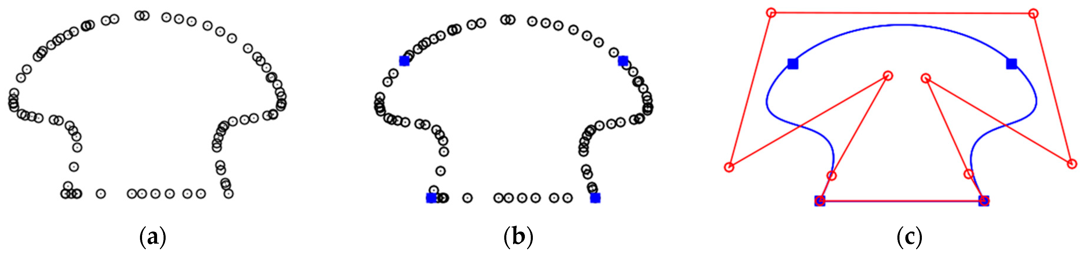
The first term in Equation (1) is related to CD-splines basis functions (Ni,D) with elements computed considering the degree of the polynomial (di), knot points, and continuity type between connected adjacent segments. The degree of the polynomial is an integer value and is related to the degree of the polynomial used to model each segment, whereas the knot points are responsible for identifying the beginning and end of each segment. The type of continuity corresponds to the curvature at the joining point between two adjacent segments. The second term (Pi) is formed by control points, which controls the shape of the curve and is determined through an estimation process. Figure 1 shows an example of modeled contour (blue line) using the CD-spline approach. In this example, the boundary points are represented by hollow black circles, whereas the knot points are symbolized by solid blue squares, and the control points are represented by hollow red circles.
Assuming that one set of m+1 points in 3D space is available, i.e., (), these points can be represented by the vector (Equation (2)), with .
Equation (3) presents the chord length formulation, which is considered to parameterize the coordinates of the piecewise polynomial function C(t).
where:
The CD-splines basis functions are defined over a knot vector () and a degree vector (). For CD-spline basis functions, it is necessary to know the polynomial degree for each interval between each knot element, defining a segment. Considering that = {ui} is a non-decreasing real number sequence and = {di} is bounded by positive integer sequence, Shen and Wang [25] imposed the following constraint on these two sequences:
If , then and .
For , where , CD-spline basis functions are defined over and vectors.
The control points are estimated utilizing the least-squares adjustment concept (Equation (7)). In this context, the error function presented in Equation (6) is considered [26]. It is assumed that all segments have order continuity 0 (), i.e., all neighboring segments meet at the same point.
The vector is obtained by Equation (2), whereas the matrix is defined by the following formulation:
3. Proposed Method
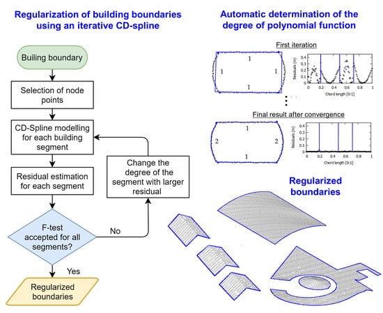
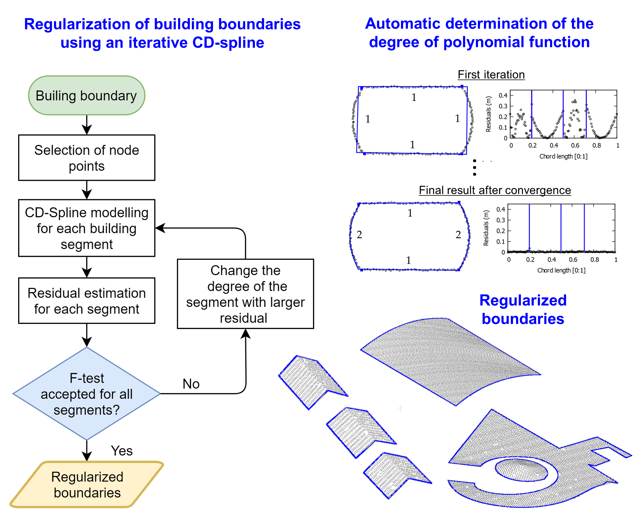
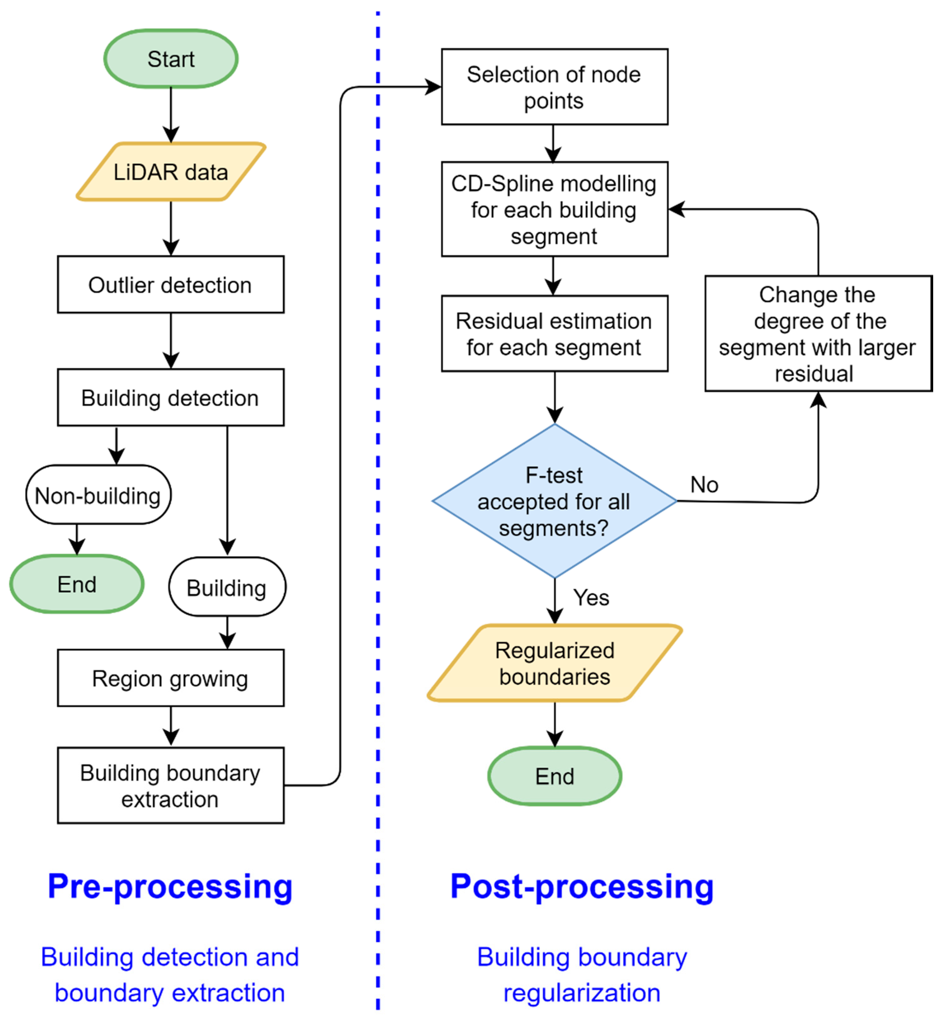
A simplified flowchart of the proposed strategy is shown in Figure 2, which is divided into two main steps. The first step involves building detection and boundary extraction. In the second step, the building boundary regularization is performed using an iterative implementation of the CD-spline, while using a stopping criterion that is based on residual analysis through an F statistical test. In sequence, the different steps of the proposed method are described.
3.1. Building Detection and Boundary Extraction
The LiDAR data may contain undesired outliers, e.g., extremely high and/or low points, due to external factors present in the scene [27,28]. In order to detect and eliminate such outliers, the proposed approach by Carrilho et al. [29] was used. Designated as cell histogram filter, the approach aims at identifying outlier points through an analysis of a locally generated height frequency histogram. The separation between the ground and non-ground points was performed using the progressive TIN (Triangulated Irregular Network) densification strategy proposed by Axelsson [30] and implemented in the lasground tool of LAStools (http://rapidlasso.com/lastools/). This is an iterative method that can work directly on the raw point cloud.
To obtain the set of the points corresponding to each grouping within non-ground points, a region growing strategy was implemented. The region growing was executed in the spatial domain using an approach similar to the one presented by Sampath and Shan [14]. In this process, two thresholds were adopted [31]: planimetric distance () and altimetric distance (). The identification of building groupings was carried out using the method proposed by Santos et al. [31], which considers the entropy concept to determine the attributes related to each cluster, and the k-means algorithm to perform automatic classification considering two classes: building and vegetation. The advantage of this approach is the automatic identification of clusters, dispensing the need for a training step.
The building boundary extraction was performed on the point cloud clustering derived from the k-means algorithm. The approximate boundaries were extracted using the adaptive alpha-shape algorithm approach [32], which is a variant of the original alpha-shape algorithm presented by Edelsbrunner et al. [20]. The general idea of the algorithm consists of the use of an alpha parameter to identify pairs of points that compose each edge segment of the object. In Santos et al. [32], this parameter is estimated automatically based on local point spacing. In Figure 3, we show an example of the results derived from the separation between ground and non-ground (Figure 3b), region growing (Figure 3c), building cluster detection (Figure 3d,e), and building boundary extraction (Figure 3f).
3.2. Regularization Using the Proposed Iterative CD-Spline
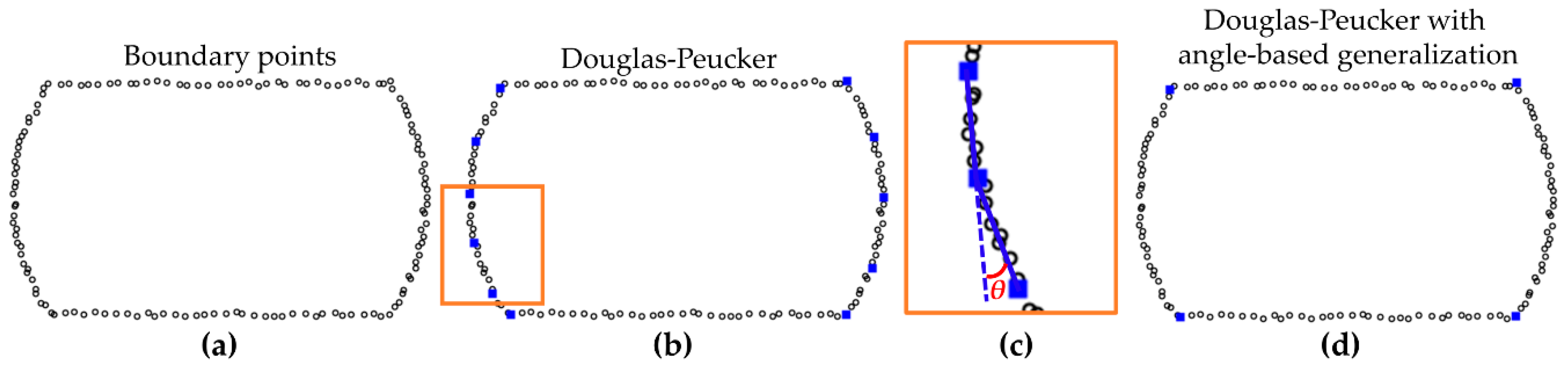
The determination of the parametric curve using the original CD-spline from Equation (1) is performed in a single iteration. In this sense, it is necessary to have a priori knowledge of the following information: boundary points, critical points, and degree of the function used to model each segment. In this work, the boundary points were obtained using the adaptive alpha-shape algorithm approach proposed by Santos et al. [32], whereas the critical points were determined using the well-known Douglas–Peucker algorithm, followed by angle-based generalization, similar to Lee et al. [15]. Douglas–Peucker was executed in the tridimensional space using a distance threshold () followed by the elimination of redundant critical points while applying an angle threshold (). In the angle-based generalization step, we calculate the angles between two adjacent lines formed by connecting adjacent critical points. If the angle is smaller than the angle threshold (), the point is regarded as a redundant point and is discarded. Figure 4 shows an example of the results derived from critical point determination step. In Figure 4a only the boundary points (black dots) are displayed, whereas in Figure 4b,d the critical points (blue squares) derived from Douglas–Peucker algorithm and angle-based generalization are shown, respectively. In Figure 4c the geometric representation of the angle θ between two adjacent lines (blue lines) is shown.
In order to automatically determine the degree of polynomial, an iterative CD-spline modeling was proposed. The strategy adopted for polynomial degree evaluation is based on significance analysis of residuals for each segment, within an iterative CD-spline process. In the first iteration, all segments are modeled by a first-degree polynomial. After this modeling, the residuals for each boundary point are estimated and the sum of residuals for each segment is determined. The degree of the segment that has the biggest sum of residuals is increased by one. In the following iterations, the boundary is modeled considering the new polynomial degree for the segment with the largest sum of residuals. The process is repeated until there is no significant difference between the modeled boundaries between two successive iterations k−1 and k, while using a prespecified level of significance (α).
To verify whether the difference between two successive iterations is significant, the statistical F-test was used [33,34], by comparing the standard deviation of absolute residuals between these iterations. In the following, we present all the steps of the iterative CD-spline approach:
Step 1—All segments are modeled by a polynomial of degree 1 (straight lines);
Step 2—The CD-spline is performed over the boundary points to obtain the regularized boundary (modeled boundary);
Step 3—For each point, in a given segment, the magnitude of the residual (rj) is estimated using
Equation (9):
Step 4—The sum of the all rj for each segment is computed, with each segment defined by the critical points (knot points);
Step 5—The degree of the polynomial function related to the segment with largest sum is increased by one;
Step 6—If it is the first iteration return to Step 2. Otherwise, go to Step 7;
Step 7—A statistical F-test is conducted using the estimated statistic () (Equation (10))
computed considering the standard deviations of residuals in iteration k and k − 1, respectively; compared to the theoretical statistics (, ), based on the number of boundary points (n) and level of significance (α), until the stopping criterion has been met, as can be seen in [33,34]:
Step 8—The process is finished. Regularized boundary obtained in iteration k − 1 is adopted as the final result.
In Equation (10) the standard deviations of residuals, corresponding to iteration k and k − 1, i.e., and respectively, are computed considering all boundary points.
In Figure 5, intermediate steps of the proposed iterative CD-spline are illustrated for one building with segments that are modeled by different degree polynomials, i.e., two straight-line and two curved segments. For each iteration, the following information are presented: boundary points (black points), critical points (blue square, indicated by blue arrows), regularized boundary using the CD-spline approach (blue line), the degree of the polynomial for each segment (number adjacent to each segment), and residual plot. In this figure, the blue vertical lines delimit the set of points corresponding to each segment. In this example, as can be seen in Figure 5, four iterations were required to model the contour of this building. In the first iteration, all segments were modeled by a polynomial function of degree 1 (straight-line segment). In the second iteration, the segment corresponding to the highest sum of the magnitude of residuals was modeled by a polynomial of degree 2. In this case, the regularized contour obtained in the third iteration (Figure 5c) was adopted as the final result, since there is no significant improvement in the fourth iteration (Figure 5d).
3.3. Quality Parameters
The assessment of the regularized building boundaries was performed both qualitatively and quantitatively. The qualitative analysis was carried out through a visual inspection, whereas the quantitative analysis was performed using quality parameters, such as Fscore, PoLiS metric, and root mean squared error (RMSE) estimated for each boundary segment and then for each building. For details related to these quality indicators, interested readers can refer to [35,36,37]. To perform the quantitative analysis, the boundary extracted by the proposed method was compared with the reference boundary for two datasets. For the first dataset, the reference boundary was manually generated from aerial images using a photogrammetric restitution procedure on an ERDAS IMAGINE LPS system (version 2015). For the second dataset, the reference boundary was available, as described in Section 4.
Assuming an extracted polygon () and the reference polygon (), Fscore can be obtained through the harmonic average between recall and precision, that can also be directly computed from true positive (TP), false positive (FP), and false negative (FN) using:
where is the measured area; = A∩B; = ar(B) − A∩B; and = ar(A) − A∩B.
The PoLiS metric between two polygons and is defined by Equation (12) [37]:
where and correspond to the number of vertices of polygons and , respectively; and denote the boundary of polygons and , respectively; and is the Euclidean distance between points and .
The values of the PoLiS range from 0 to +. When the value approaches zero, it is an indicator that the extracted boundary approaches the reference boundary.
4. Datasets
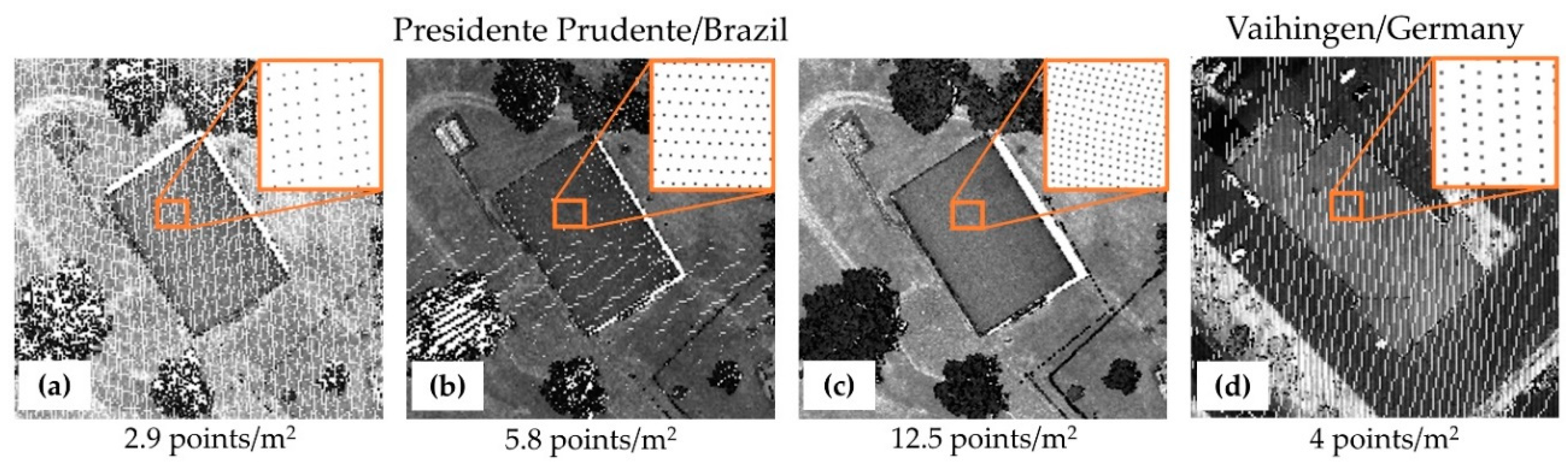
The experiments were performed using two airborne LiDAR datasets. The first dataset was generated from three different flying heights over the city of Presidente Prudente/Brazil by Sensormap Geotecnologia, as described in [38]. The point clouds were acquired from average flying heights of 1300, 900, and 550 m, resulting in point densities of approximately 2.9, 5.8, and 12.5 points/m2 (Figure 6a–c), respectively. The airborne LiDAR system used in the acquisition was the RIEGL LMS-Q680i. The second dataset comes from the ISPRS Test Project on Urban Classification, 3D Building Reconstruction and Semantic Labeling, which was captured over Vaihingen/Germany [39]. This second dataset was acquired at an average flying height of 500 m using a Leica ALS50 system with an average point density of 4 points/m2 (Figure 6d).
5. Boundary Regularization Results
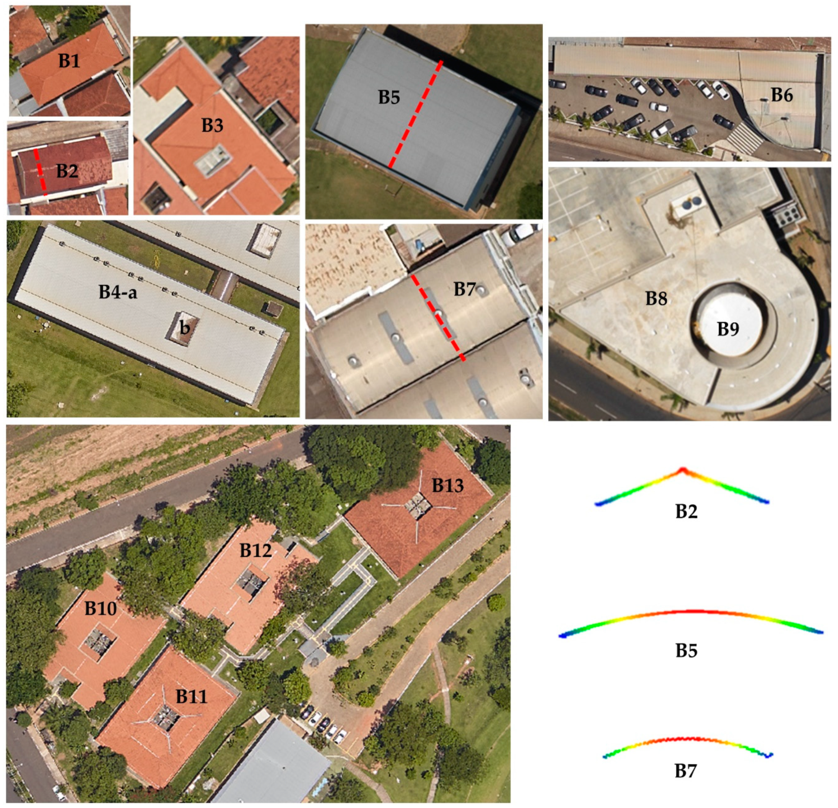
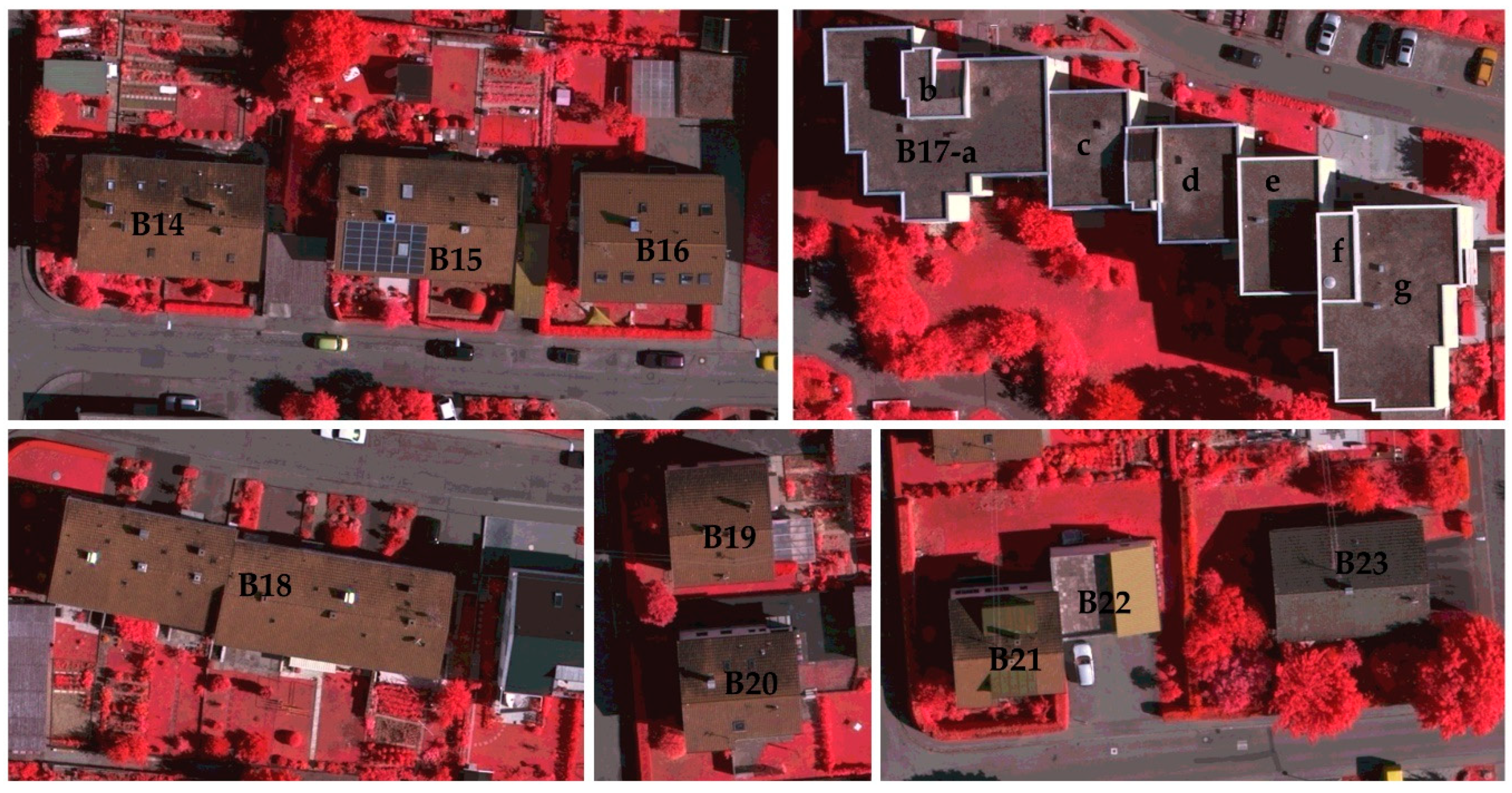
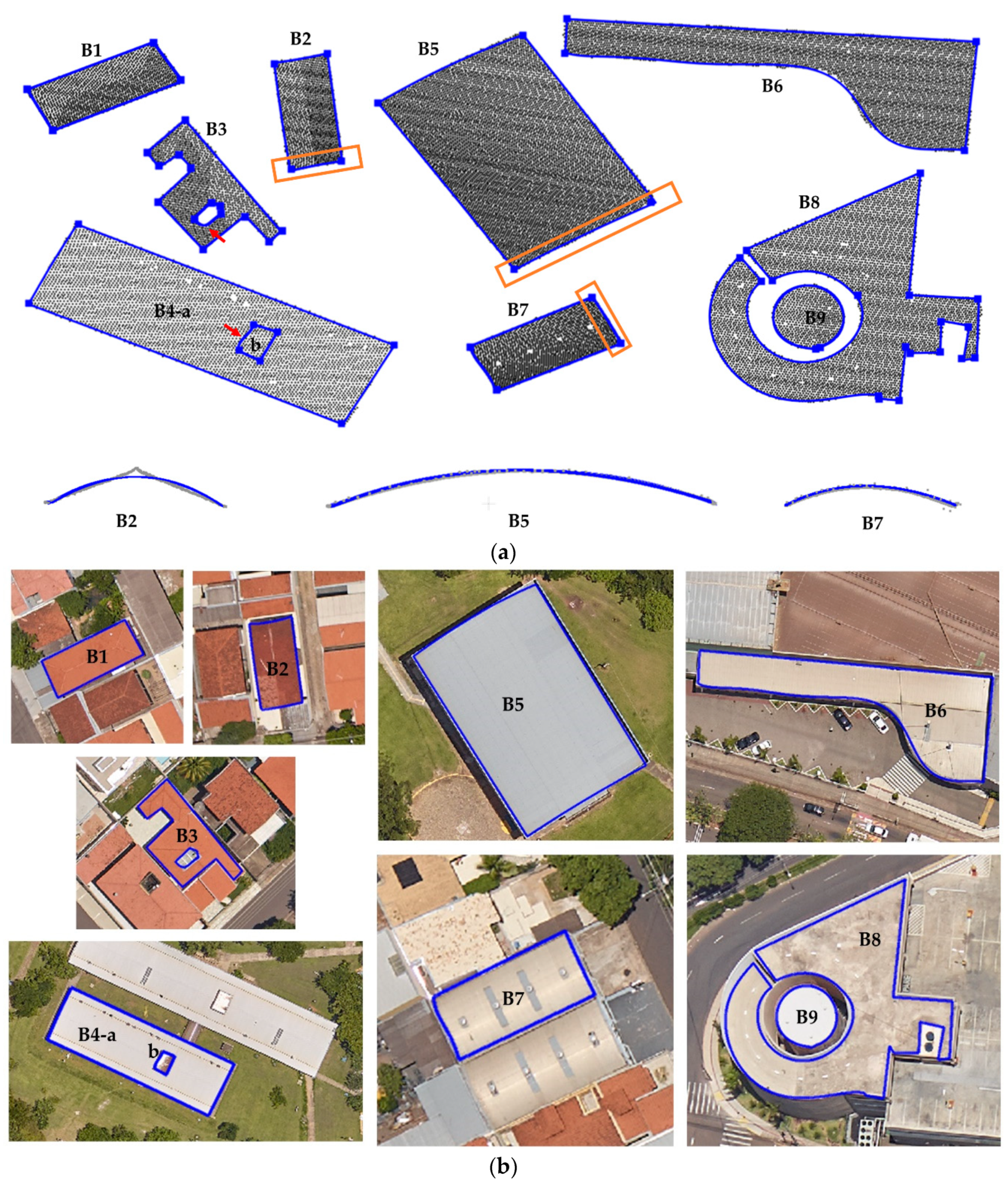
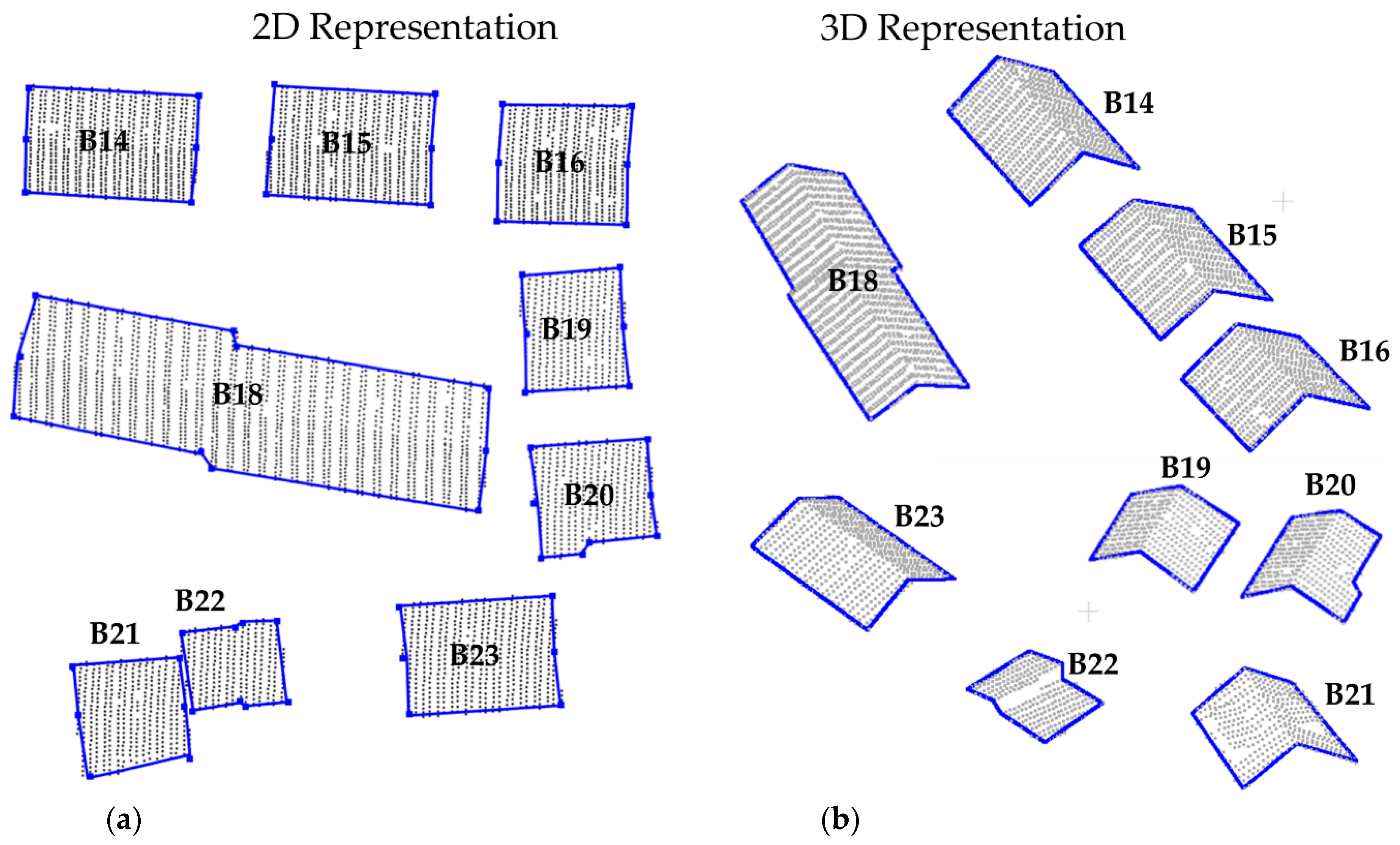
The proposed strategy was evaluated considering several scenarios, such as using different regularization parameters, buildings with different complexities, datasets with varying point density, and buildings with vegetation occlusion. The experiments were executed considering buildings selected from Presidente Prudente/Brazil (Figure 7) and Vaihingen/Germany (Figure 8) datasets. Buildings B1 and B4 correspond to simple buildings of rectangular shape with different dimensions. Building B2 is composed of a gable roof, producing an inverted "V" shaped contour, as shown in the corresponding profile. Building B3 has a more complex shape, which is composed of straight-line segments of different sizes and a hole in the middle of the roof. Buildings B5 and B7 are formed by a curved roof, as can be seen in both profiles. Building B6 is made up of straight-line and curved segments. Building B8 has a highly complex boundary, having straight-line and curved segments of different dimensions. For this building, the curved part resembles a spiral. Building B9 has a circular shape, whereas buildings B10, B11, B12, and B13 have vegetation at their surroundings. In contrast, the buildings of Vaihingen/Germany dataset have less complex contour (Figure 8). Buildings B14–B23 have a rectangular shape, being B14–B16, B18–B21, and B23 with gable roofs. Building 17 consists of several roofs with different heights.
In the proposed method, thresholds are used during pre-processing and post-processing steps. In pre-processing, the values of and were defined according to [31]. As the focus of the work is the regularization, the following discussion provide a detailed analysis of the thresholds used in the post-processing/regularization stage.
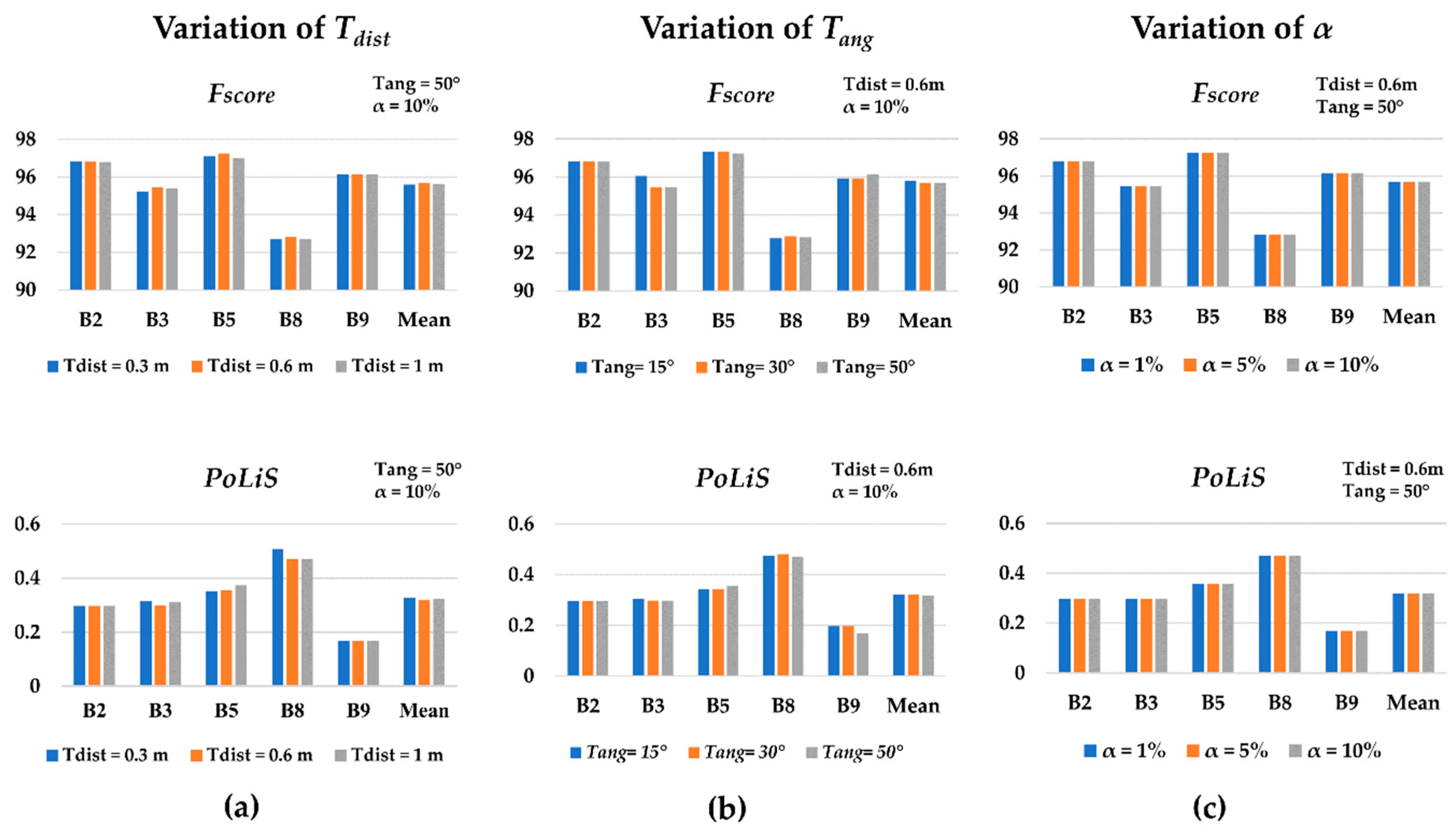
In the regularization process, it is necessary to define three different thresholds: Tdist, Tang, and α (level of significance). To verify the influence of such parameters, the proposed strategy was executed considering different configurations. For each configuration, we estimated the Fscore and PoLiS metrics, as can be seen in Figure 9a–c. These metrics were carried out considering five buildings (B2, B3, B5, B8, and B9), selected from the point cloud with 12.5 points/m2. In the first configuration (Figure 9a), Tdist assumed the following values: 0.3, 0.6, and 1 m, whereas Tang and α are kept fixed to 50° and 10%, respectively. In Figure 9b the parameter Tang assumes the values 15°, 30°, and 50°, whereas Tdist and α are constant, 0.6 m and 10%, respectively. Finally, Figure 9c shows the results related to variation of the level of significance (α): 1%, 5%, and 10% with Tdist and Tang set to 0.6 m and 50°, respectively. Figure 10a,b shows the final results for buildings B2, B8, and B9 using different values of Tang.
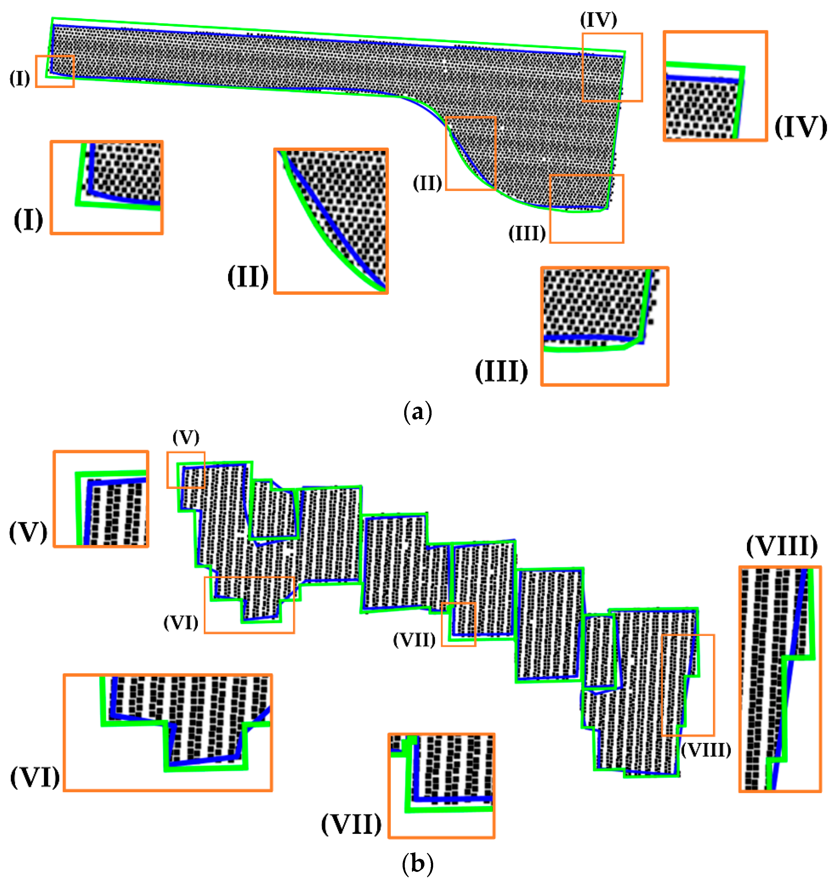
To evaluate the regularization process for different types of buildings, buildings B1–B9 and B14–B23 were considered (Figure 7 and Figure 8). The building boundaries of buildings B1–B9 were derived from point cloud with a density of 12.5 points/m2, the following regularization parameters being used: = 0.60 m, = 50°, and α = 10%. For buildings B14–B23 the following values were considered: = 0.80 m, = 40°, and α = 10%. In Figure 11 the regularized boundaries for Presidente Prudente/Brazil dataset are shown, whereas in Figure 12 and Figure 13 the results corresponding to Vaihingen/Germany dataset are shown. The estimated quality parameters for selected buildings, as well as the average value of each metric are shown in Table 1. In Figure 14, we show the reference and regularized boundary for buildings B6 and B17 with highlighted discrepancies between the contours. In the Presidente Prudente/Brazil dataset, the reference boundaries were derived from images with 10 cm ground sampling distance (GSD), resulting in contours with accuracy around 16 cm in planimetry and 22 cm in altimetry. In the Vaihingen/Germany dataset, images with 8 cm were used, obtaining reference contours with accuracy around 10 cm in planimetry and altimetry [40].
The regularization process may be affected by different factors, among them are point density and occlusion caused by vegetation. To verify the robustness of the proposed approach while using point clouds with different point density, the strategy was applied to buildings B5, and B7–B9, which were selected from the available point clouds, as shown in Figure 15. To verify the impact of potential occlusions by vegetation, buildings B10–B13 were considered (Figure 16). The results in Figure 15 and Figure 16 were generated considering the following thresholds: = 0.60 m, = 50°, and α = 10%.
As can see in Figure 2, we divided the method in pre-processing and post-processing steps. Since the aim of the paper was focused on the introduction of the proposed approach, we do not focus on discussing and evaluating the performance in terms of processing time. In fact, the processing time is function of the hardware, software, and available data. The pre-processing step was implemented in ANSI C language, compiled in Code: Block IDE. In this step, the LAStools was used in one part, as explained in Section 3.1. The post-processing step was implemented in GNU Octave environment. All the experiments were processed in one notebook running with Intel core i7-5500 U processor at 2.4 GHz, 64-bits, 8 GB RAM, and 500 GB disk. Considering the region shown in Figure 3 with 175.151 points and density of 12 points/m2, the total processing time was 243 s. This result indicates that the elapsed time was around 2.31 min/100k points. It is relevant to mention that this number can be modified by optimizing the software and changing the platform. Besides, the processing time is also affected by the point cloud density, number of buildings, and the complexity of the buildings.
6. Discussion of Results
Considering the results in Figure 9a, the variation of the Tdist threshold did not produce significant changes in the quality metrics. This is an indication that the regularization process has similar results using different values of Tdist.
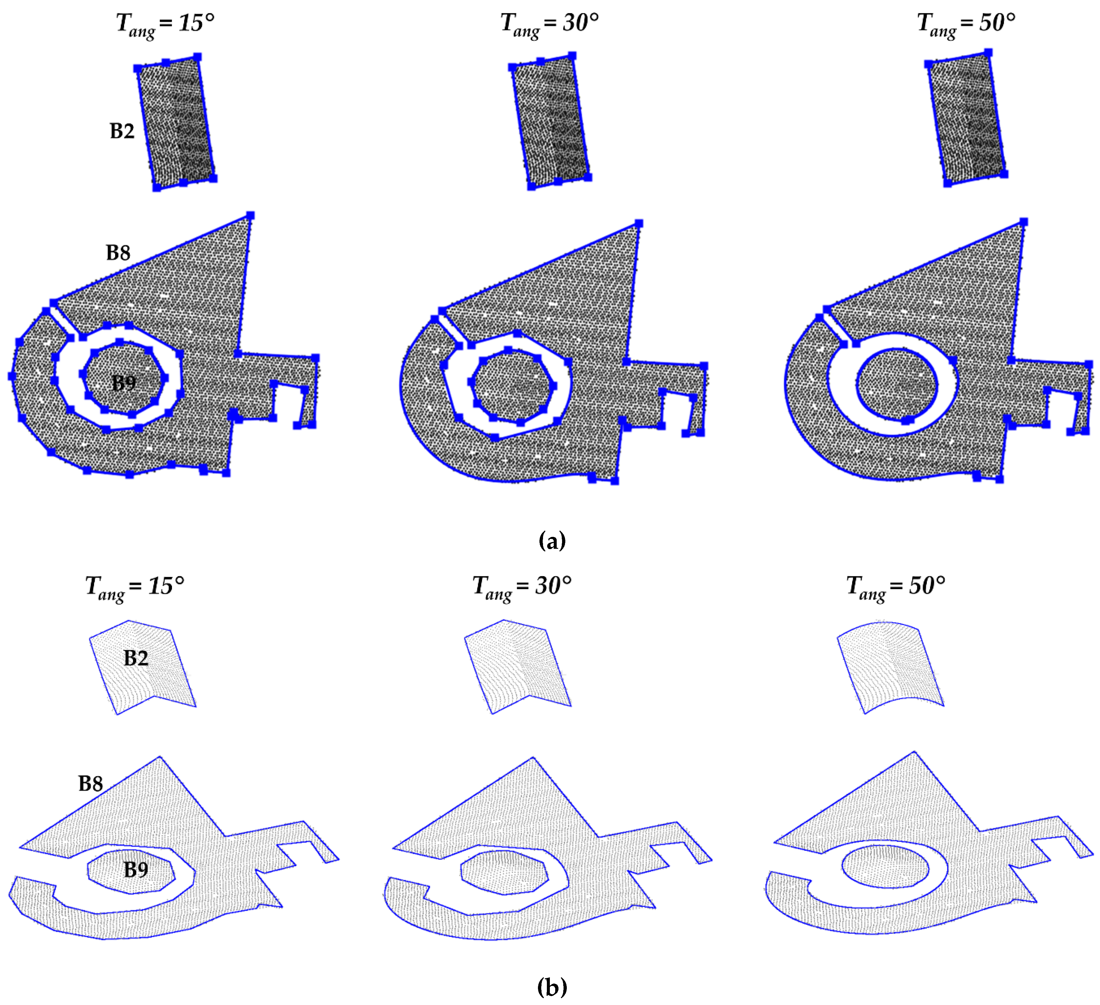
In terms of the mean value of Fscore, Tang of 15° leads to the best value (Figure 9b). Concerning the average value of the PoLiS metric, Tang of 50° correspond to the best result. Despite this, the quality parameters did not show significant variation using different values of Tang. Performing a visual analysis of the results in Figure 10a, it is possible to notice that several corner points were identified on the curved segment when using Tang of 15° and 30°. In these cases, the curved contour was modeled by several small segments of straight lines instead of a curve. The use of Tang of 50° allowed the correct modeling of the curved contours, however, the corner point of segment “V” was not identified and consequently was represented by a curved segment. Therefore, it is noted that the Tang parameter has a direct influence on the selection of corner points and consequently on the determination of the type of polynomial function used to model the contour.
In Figure 9c, it is possible to observe that the quality metrics related to the three values of significance level were identical. These results indicate that the proposed approach is not sensitive to the significance level values considered (α = 1%, α = 5%, and α = 10%).
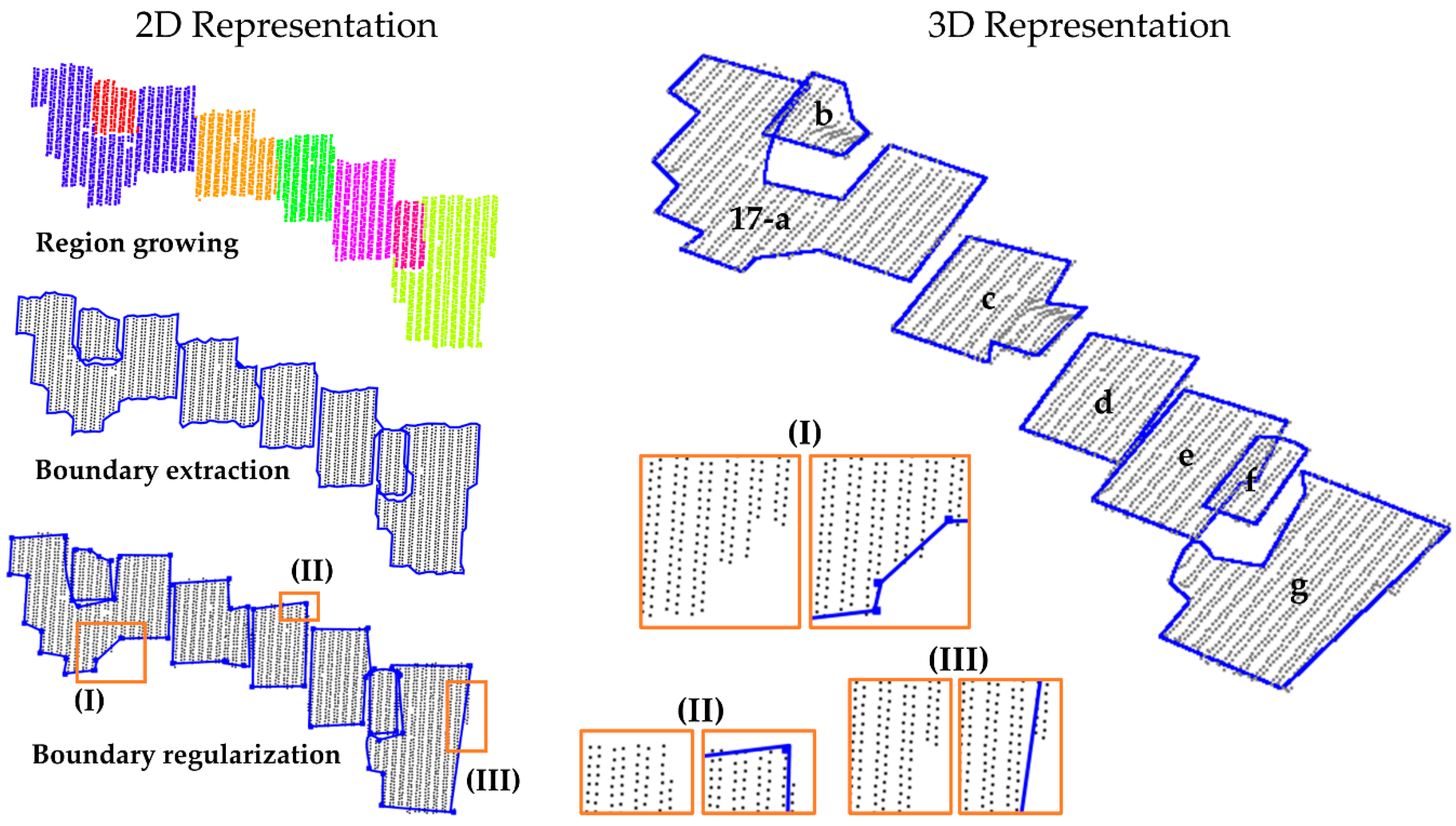
From the visual analysis of the results in Figure 11, Figure 12 and Figure 13, it can be seen that most of the corner points were correctly determined. In general, the regularization method produced consistent results, since straight-line and curved segments were properly modeled, as can be seen in Figure 11, Figure 12 and Figure 13. Even in the case of complex boundaries (B3, B5, B8, and B9), the method behaved robustly. However, the method had problems modeling small segments, as can be observed in Figure 11 (distinguished by the small arrows), since two small segments were not properly extracted for buildings B3 and B4-b. In both cases, the distinguished segments were modeled by a curved segment, instead of a straight-line. In Figure 13, it is observed that the different roof levels of building B17 were correctly identified, allowing to model each roof contour separately. However, some modeling problems occurred in B17, which are related to small details (Figure 13-I, Figure 13-III, and Figure 14b-VIII) and some rectangular edges (Figure 13-II, Figure 14b-VI). In Figure 14, one can observe some discrepancies between reference and regularized boundaries, which result from the modeling of segments and corners. From these results, it is possible to conclude that the proposed strategy has the potential to model building boundaries with different complexities, despite having limitations when dealing with small segments.
The modeling of the building with gable roof (B2) presented some inconsistencies. In Figure 11a, one can see that important corner points were not identified. In this case, the “V” shape of the boundary was modeled as a curved segment rather than two straight lines. This problem is related to the selected Tang threshold used for the critical point determination process, as highlighted in Figure 10. By changing this threshold to a smaller value, Tang = 30° for example, the corners points are correctly extracted (Figure 10a). In contrast, all gable roofs (B14–B16, B18–B21, and B23) were correctly modeled in the Vaihingen/Germany dataset, as can be seen in Figure 12b. In this case, it was adopted Tang = 40° in the regularization process.
In terms of the Fscore metric (Table 1), building B1 has the best value of 98.8%, and building B22 has the worst value of 91.5%. Buildings composed of curved segments presented an average Fscore value of 95.5%, against 95.4% for other buildings. In general, the average Fscore value was around 95%. These values indicate that modeling quality was similar for different types of buildings, and there is a high agreement between the regularized results and the reference boundaries.
Comparing the RMSE values for the derived boundaries with the reference ones (Table 1), one can verify that the best RMSE value of around 0.08 m corresponds to the Z component. This result was expected since LiDAR data has better accuracy in altimetry. For the XY coordinates, the proposed strategy produced a mean RMSE value of 0.17 m. The metric PoLiS, which is directly related to RMSE, has an average value of around 0.30 m. For buildings with some type of curved segments, the average PoLiS was 0.31 m, against 0.30 m for other buildings. These values indicate the potential of the proposed method in modeling building boundaries of different complexities.
Considering the results using point clouds with different densities (Figure 15), it can be observed that the proposed strategy was able to model boundaries regardless of point cloud density. In general, curved segments were correctly modeled, including those of building B8 which has a complex shape. As expected, comparing the results in Figure 15g,i, one can observe the limitation of using a lower density point cloud when modeling small details. These results indicate the robustness of the proposed method when working with point clouds of different densities.
In Figure 16, it is possible to notice that the presence of vegetation near the building roof can cause occlusions (information loss), or even the grouping of vegetation points in the building class. In these regions, the modeled boundary presented irregular shape, i.e., different than expected. In spite of this, the proposed method was able to model the complete building boundaries producing correct results in the regions free of vegetation. Although not explored in this paper, the proposed strategy can be improved by applying selective corner points estimation in such areas.
In summary, the qualitative and quantitative analysis indicates that the proposed strategy has the potential to model different types of boundaries, including boundaries formed by curved segments with different complexity.
Criteria for Threshold Selection
The proposed method makes use of some thresholds, whose values must be carefully selected in order to achieve the desired results. Table 2 provides a brief summary of the thresholds considered in pre-processing and post-processing steps, the elements considered in prediction, and possible negative impacts. Among the possibilities to derive their values, the suggested ones are based on the available data which can be either measured, computed, or assessed from the point cloud.
7. Conclusions
This paper proposes a method for building roof boundary extraction from airborne LiDAR data. The main contribution is related to the use of an iterative approach of CD-spline, which makes it possible to automatically select the degree of the polynomial function that models each segment. This method is robust in modeling boundaries with different levels of complexities, including buildings composed of complex curved segments and point clouds with different densities. In general, the proposed method presented Fscore and PoLiS around 95% and 0.30 m, respectively. The drawback of the proposed strategy is directly related to the process of corner point selection, since boundary details can be missed.
The proposed strategy generates accurate building boundaries but there are some sources of errors that can affect the results, such as occlusions caused by vegetation, and inaccurate initial boundary. Therefore, the integration of LiDAR data and imagery will be considered to improve the accuracy and to mitigate some occlusion problems. Moreover, we will explore a more robust procedure for corner point determination.
Author Contributions
Conceptualization methodology and validation, R.C.d.S., M.G., and A.F.H.; methodology implementation, R.C.d.S.; writing—original draft preparation, R.C.d.S.; writing—review and editing, R.C.d.S, M.G. and A.F.H.; M.G. and A.F.H. supervised this study. All authors have read and agreed to the published version of the manuscript.
Funding
This research was funded by São Paulo Research Foundation—FAPESP (grants no. 2016/12167-5, no. 2016/20814-0 and no. 2019/05268-8) and National Council for Scientific and Technological Development—CNPq (grants no. 304189/2016-2 and no. 308474/2019-8).
Acknowledgments
The authors would like to thank Graduate Program on Cartographic Sciences from FCT-UNESP, Presidente Prudente/Brazil; Digital Photogrammetry Research Group (DPRG) at Purdue University; Sensormap Geotecnologia for providing the LiDAR data from Presidente Prudente/Brazil and also the German Society for Photogrammetry, Remote Sensing and Geoinformation (DGPF) for providing the Vaihingen/Germany dataset. São Paulo Research Foundation—FAPESP (grants no. 2016/12167-5, no. 2016/20814-0 and no. 2019/05268-8) and National Council for Scientific and Technological Development—CNPq (grants no. 304189/2016-2 and no. 308474/2019-8) for supporting this research.
Conflicts of Interest
The authors declare no conflict of interest.
References
- The United Nations—Department of Economic and Social Affairs. 2018. Available online: https://www.un.org/development/desa/en/news/population/2018-revision-of-world-urbanization-prospects.html (accessed on 28 December 2018).
- Kwak, E.; Habib, A. Automatic Representation and Reconstruction of DBM from LiDAR Data Using Recursive Minimum Bounding Rectangle. ISPRS J. Photogramm. Remote Sens. 2014, 93, 171–191. [Google Scholar] [CrossRef]
- Jung, J.; Jwa, Y.; Sohn, G. Implicit Regularization for Reconstructing 3D Building Rooftop Models Using Airborne LiDAR Data. Sensors 2017, 17, 621. [Google Scholar] [CrossRef] [PubMed]
- Xie, L.; Zhu, Q.; Hu, H.; Wu, B.; Li, Y.; Zhang, Y.; Zhong, R. Hierarchical Regularization of Building Boundaries in Noisy Aerial Laser Scanning and Photogrammetric Point Clouds. Remote Sens. 2018, 10, 1996. [Google Scholar] [CrossRef] [Green Version]
- Zheng, Y.; Weng, Q.; Zheng, Y. A Hybrid Approach for Three-Dimensional Building Reconstruction in Indianapolis from LiDAR Data. Remote Sens. 2017, 9, 310. [Google Scholar] [CrossRef] [Green Version]
- Kedzierski, M.; Fryskowska, A. Methods of Laser Scanning Point Clouds Integration in Precise 3D Building Modelling. Measurement 2015, 74, 221–232. [Google Scholar] [CrossRef]
- Kedzierski, M.; Fryskowska, A. Terrestrial and Aerial Laser Scanning Data Integration Using Wavelet Analysis for the Purpose of 3D Building Modeling. Sensors 2014, 14, 12070–12092. [Google Scholar] [CrossRef] [Green Version]
- Fischer, A.; Kolbe, T.H.; Lang, F.; Cremers, A.B.; Förstner, W.; Plümer, L.; Steinhage, V. Extracting Buildings from Aerial Images Using Hierarchical Aggregation in 2D and 3D. Comput. Vis. Image Underst. 1998, 72, 185–203. [Google Scholar] [CrossRef] [Green Version]
- Manno-Kovacs, A.; Sziranyi, T. Orientation-Selective Building Detection in Aerial Images. ISPRS J. Photogramm. Remote Sens. 2015, 108, 94–112. [Google Scholar] [CrossRef]
- Wang, J.; Yang, X.; Qin, X.; Ye, X.; Qin, Q. An Efficient Approach for Automatic Rectangular Building Extraction from Very High Resolution Optical Satellite Imagery. IEEE Geosci. Remote Sens. Lett. 2015, 12, 487–491. [Google Scholar] [CrossRef]
- Kim, C.; Habib, A. Object-Based Integration of Photogrammetric and LiDAR Data for Automated Generation of Complex Polyhedral Building Models. Sensors 2009, 9, 5679–5701. [Google Scholar] [CrossRef]
- Du, S.; Zhang, Y.; Qin, R.; Yang, Z.; Zou, Z.; Tang, Y.; Fan, C. Building Change Detection Using Old Aerial Images and New LiDAR Data. Remote Sens. 2016, 8, 1030. [Google Scholar] [CrossRef] [Green Version]
- Gilani, S.; Awrangjeb, M.; Lu, G. An Automatic Building Extraction and Regularisation Technique Using LiDAR Point Cloud Data and Orthoimage. Remote Sens. 2016, 8, 258. [Google Scholar] [CrossRef] [Green Version]
- Sampath, A.; Shan, J. Building Boundary Tracing and Regularization from Airborne Lidar Point Clouds. Photogramm. Eng. Remote Sens. 2007, 73, 805–812. [Google Scholar] [CrossRef] [Green Version]
- Lee, J. Extraction and Regularization of Various Building Boundaries with Complex Shapes Utilizing Distribution Characteristics of Airborne LIDAR Points. ETRI J. 2011, 33, 547–557. [Google Scholar] [CrossRef]
- Jochem, A.; Höfle, B.; Rutzinger, M.; Pfeifer, N. Automatic Roof Plane Detection and Analysis in Airborne Lidar Point Clouds for Solar Potential Assessment. Sensors 2009, 9, 5241–5262. [Google Scholar] [CrossRef] [PubMed]
- Satari, M.; Samadzadegan, F.; Azizi, A.; Maas, H.-G. A Multi-Resolution Hybrid Approach for Building Model Reconstruction from Lidar Data: A Multi-resolution Hybrid Approach for Building Model Reconstruction. Photogramm. Rec. 2012, 27, 330–359. [Google Scholar] [CrossRef]
- Albers, B.; Kada, M.; Wichmann, A. Automatic Extraction and Regularization of Building Outlines from Airborne LiDAR Point Clouds. Int. Arch. Photogramm. Remote Sens. Spat. Inf. Sci. 2016, XLI-B3, 555–560. [Google Scholar] [CrossRef]
- dos Santos, R.C.; Galo, M.; Carrilho, A.C. Building Boundary Extraction from LiDAR Data Using a Local Estimated Parameter for Alpha Shape Algorithm. Int. Arch. Photogramm. Remote Sens. Spat. Inf. Sci. 2018, XLII-1, 127–132. [Google Scholar] [CrossRef] [Green Version]
- Edelsbrunner, H.; Kirkpatrick, D.; Seidel, R. On the Shape of a Set of Points in the Plane. IEEE Trans. Inf. Theory 1983, 29, 551–559. [Google Scholar] [CrossRef] [Green Version]
- Maas, H.-G.; Vosselman, G. Two Algorithms for Extracting Building Models from Raw Laser Altimetry Data. ISPRS J. Photogramm. Remote Sens. 1999, 54, 153–163. [Google Scholar] [CrossRef]
- Xu, J.; Wan, Y.; Yao, F. A Method of 3D Building Boundary Extraction from Airborne LIDAR Points Cloud. In Proceedings of the 2010 Symposium on Photonics and Optoelectronics, Chengdu, China, 19–21 June 2010; pp. 1–4. [Google Scholar]
- Awrangjeb, M. Using Point Cloud Data to Identify, Trace, and Regularize the Outlines of Buildings. Int. J. Remote Sens. 2016, 37, 551–579. [Google Scholar] [CrossRef]
- Chen, X.; Yu, K. Feature Line Generation and Regularization from Point Clouds. IEEE Trans. Geosci. Remote Sens. 2019, 57, 9779–9790. [Google Scholar] [CrossRef]
- Shen, W.; Wang, G. Changeable Degree Spline Basis Functions. J. Comput. Appl. Math. 2010, 234, 2516–2529. [Google Scholar] [CrossRef] [Green Version]
- Bartels, R.H.; Beatty, J.C.; Barsky, B.A. An Introduction to Splines for Use in Computer Graphics and Geometric Modeling; Morgan Kaufmann: Burlington, MA, USA, 1995. [Google Scholar]
- Irad, B.-G. Outlier Detection, Data Mining, and Knowledge Discovery Handbook: A Complete Guide for Practitioners and Researchers; Kluwer Academic Publishers: Berlin, Germany, 2005. [Google Scholar]
- Rashidi, A.; Brilakis, I. Point Cloud Data Cleaning and Refining for 3D As-Built Modeling of Built Infrastructure. In Proceedings of the Construction Research Congress 2016, San Juan, Puerto Rico, 31 May–2 June 2016; pp. 919–929. [Google Scholar]
- Carrilho, A.C.; Galo, M.; Santos, R.C. Statistical Outlier Detection Method for Airborne LiDAR Data. ISPRS Int. Arch. Photogramm. Remote Sens. Spat. Inf. Sci. 2018, XLII-1, 87–92. [Google Scholar] [CrossRef] [Green Version]
- Axelsson, P. DEM Generation from Laser Scanner Data Using Adaptive TIN Models. Int. Arch. Photogramm. Remote Sens. 2000, 33, 110–117. [Google Scholar]
- Dos Santos, R.C.; Pessoa, G.G.; Carrilho, A.C.; Galo, M. Building Detection from LiDAR Data Using Entropy and the K-means Concept. ISPRS Int. Arch. Photogramm. Remote Sens. Spat. Inf. Sci. 2019, XLII-2/W13, 969–974. [Google Scholar] [CrossRef] [Green Version]
- Dos Santos, R.C.; Galo, M.; Carrilho, A.C. Extraction of Building Roof Boundaries from LiDAR Data Using an Adaptive Alpha-Shape Algorithm. IEEE Geosci. Remote Sens. Lett. 2019, 16, 1289–1293. [Google Scholar] [CrossRef]
- Mood, A.M.F.; Graybill, F.A.; Boes, D.C. Introduction to the Theory of Statistics; McGraw-Hill international editions: Statistics series; McGraw-Hill: New York, NY, USA, 1974; ISBN 978-0-07-085465-9. [Google Scholar]
- Lindgren, B.W. Statistical Theory; Collier Macmillan international editions; Macmillan: New York, NY, USA, 1976; ISBN 978-0-02-979420-3. [Google Scholar]
- Wiedemann, C.; Heipke, C.; Mayer, H.; Jamet, O. Empirical Evaluation of Automatically Extracted Road Axes. In Empirical Evaluation Techniques in Computer Vision; IEEE Computer Society Press: Los Alamitos, CA, USA, 1998; Volume 12, pp. 172–187. [Google Scholar]
- Sokolova, M.; Japkowicz, N.; Szpakowicz, S. Beyond Accuracy, F-Score and ROC: A Family of Discriminant Measures for Performance Evaluation. In AI 2006: Advances in Artificial Intelligence; Springer: Berlin/Heidelberg, Germany, 2006; pp. 1015–1021. ISBN 978-3-540-49787-5. [Google Scholar]
- Avbelj, J.; Muller, R.; Bamler, R. A Metric for Polygon Comparison and Building Extraction Evaluation. IEEE Geosci. Remote Sens. Lett. 2015, 12, 170–174. [Google Scholar] [CrossRef] [Green Version]
- Tommaselli, A.M.G.; Galo, M.; dos Reis, T.T.; da Ruy, R.S.; de Moraes, M.V.A.; Matricardi, W.V. Development and Assessment of a Data Set Containing Frame Images and Dense Airborne Laser Scanning Point Clouds. IEEE Geosci. Remote Sens. Lett. 2018, 15, 192–196. [Google Scholar] [CrossRef]
- Cramer, M. The DGPF-Test on Digital Airborne Camera Evaluation – Overview and Test Design. Photogramm. Fernerkund. Geoinf. 2010, 2010, 73–82. [Google Scholar] [CrossRef]
- Rottensteiner, F.; Sohn, G.; Gerke, M.; Wegner, J.D.; Breitkopf, U.; Jung, J. Results of the ISPRS Benchmark on Urban Object Detection and 3D Building Reconstruction. ISPRS J. Photogramm. Remote Sens. 2014, 93, 256–271. [Google Scholar] [CrossRef]
Figure 1.
Contour modeling using changeable degree (CD)-spline. Boundary points (a), knot points (solid blue squares) (b), contour obtained using the CD-spline concept (blue line) and control points (hollow red circles) (c)—adapted from Shen and Wang [25].
Figure 1.
Contour modeling using changeable degree (CD)-spline. Boundary points (a), knot points (solid blue squares) (b), contour obtained using the CD-spline concept (blue line) and control points (hollow red circles) (c)—adapted from Shen and Wang [25].

Figure 2.
Flowchart of the proposed method.

Figure 3.
Building detection and building boundary extraction. Original point cloud (a). Result derived from the separation between ground (orange) and non-ground (blue) (b). Clusters obtained from region growing (c). Separation between building and vegetation (green) (d). Building clusters (e). Building boundaries extracted using the adaptative alpha-shape algorithm (f).

Figure 4.
Determination of critical points. Boundary points (a), and critical points derived from Douglas–Peucker (blue squares) (b) and from angle-based generalization (blue squares (d). Angle θ between two adjacent lines formed by connecting adjacent critical points (c).
Figure 4.
Determination of critical points. Boundary points (a), and critical points derived from Douglas–Peucker (blue squares) (b) and from angle-based generalization (blue squares (d). Angle θ between two adjacent lines formed by connecting adjacent critical points (c).

Figure 5.
Illustration of the regularization process using the iterative approach of CD-spline. Results obtained in the first (a), second (b), third (c) and fourth (d) iteration. Black points represent the boundary points, whereas blue square and blue contours correspond to the critical points and the regularized boundary, respectively. The adjacent number to each modeled segment corresponds to the degree of the polynomial used to model this segment. The graphics illustrating the magnitude of residuals for each boundary point with each segment delimited by the vertical blue lines are also shown to the right of the modeled boundary through the different iterations.
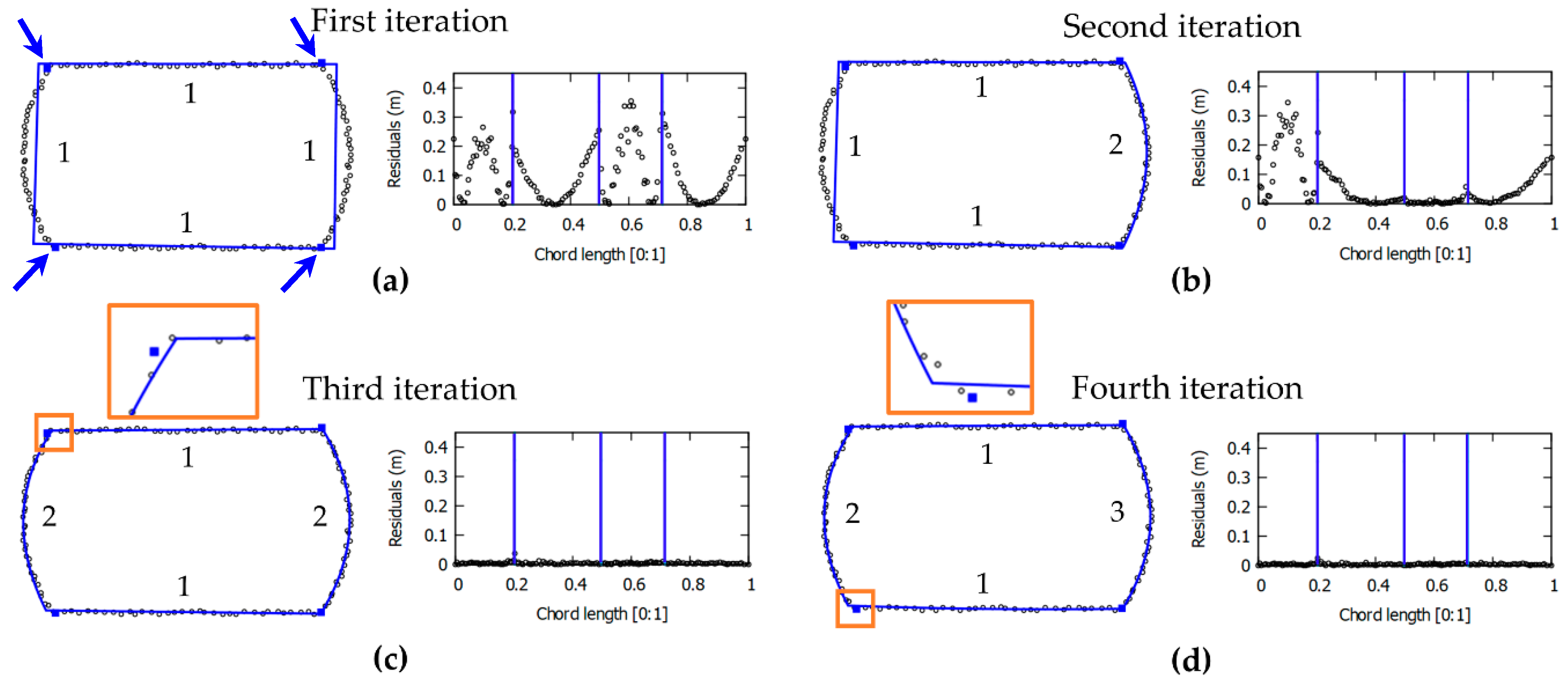
Figure 6.
Presidente Prudente/Brazil dataset: 2.9 points/m2 (a), 5.8 points/m2 (b), and 12.5 points/m2 (c). Vaihingen/Germany dataset (d).
Figure 6.
Presidente Prudente/Brazil dataset: 2.9 points/m2 (a), 5.8 points/m2 (b), and 12.5 points/m2 (c). Vaihingen/Germany dataset (d).

Figure 7.
Images of the buildings from Presidente Prudente/Brazil dataset. Buildings selected for the experiments (B1–B13) and the profiles of buildings B2, B5, and B7 generated from LiDAR point cloud.
Figure 7.
Images of the buildings from Presidente Prudente/Brazil dataset. Buildings selected for the experiments (B1–B13) and the profiles of buildings B2, B5, and B7 generated from LiDAR point cloud.

Figure 8.
Buildings selected for the experiments (B14–B23) from Vaihingen/Germany dataset.

Figure 9.
Quality parameters for buildings B2, B3, B5, B8, and B9, while varying Tdist (a), Tang (b), and level of significance (c).
Figure 9.
Quality parameters for buildings B2, B3, B5, B8, and B9, while varying Tdist (a), Tang (b), and level of significance (c).

Figure 10.
Results using different Tang values for buildings B2, B8, and B9. Representation of regularized boundaries and corner points in bidimensional space (a), and regularized boundaries in tridimensional space (b).
Figure 10.
Results using different Tang values for buildings B2, B8, and B9. Representation of regularized boundaries and corner points in bidimensional space (a), and regularized boundaries in tridimensional space (b).

Figure 11.
Presidente Prudente/Brazil dataset. Building boundary regularization results derived from the proposed strategy using a point cloud with 12.5 points/m2. Boundaries and corner points (square blue) over roof points (a), and building boundaries projected onto the aerial image (b).
Figure 11.
Presidente Prudente/Brazil dataset. Building boundary regularization results derived from the proposed strategy using a point cloud with 12.5 points/m2. Boundaries and corner points (square blue) over roof points (a), and building boundaries projected onto the aerial image (b).

Figure 12.
Vaihingen/Germany dataset. Building boundary regularization results derived from the proposed strategy. Boundaries and corner points (square blue) over roof points 2D (a) and 3D space (b).
Figure 12.
Vaihingen/Germany dataset. Building boundary regularization results derived from the proposed strategy. Boundaries and corner points (square blue) over roof points 2D (a) and 3D space (b).

Figure 13.
Building 17 in Vaihingen/Germany dataset. Results derived from region growing (top left), boundary extraction using the adaptative alpha-shape algorithm (middle left) and boundary regularization using the iterative CD-spline (bottom left). 3D representation of regularized boundaries (right).

Figure 14.
Representation of the reference (green) and regularized boundary (blue) from the proposed method for buildings B6 (a) and B17 (b).
Figure 14.
Representation of the reference (green) and regularized boundary (blue) from the proposed method for buildings B6 (a) and B17 (b).

Figure 15.
Boundary regularization results considering different point densities: 2.9 points/m2 (a,d,g), 5.8 points/m2 (b,e,h), and 12.5 points/m2 (c,f,i).
Figure 15.
Boundary regularization results considering different point densities: 2.9 points/m2 (a,d,g), 5.8 points/m2 (b,e,h), and 12.5 points/m2 (c,f,i).

Figure 16.
Buildings with vegetation in their surroundings. Boundary regularization using the proposed method over the LiDAR data (a) and corresponding aerial image (b).
Figure 16.
Buildings with vegetation in their surroundings. Boundary regularization using the proposed method over the LiDAR data (a) and corresponding aerial image (b).


Table 1.
Quality parameters using the iterative CD-spline regularization method for selected buildings from both datasets.
Table 1.
Quality parameters using the iterative CD-spline regularization method for selected buildings from both datasets.
| ID | Fscore (%) | RMSEX (m) | RMSEY (m) | RMSEZ (m) | PoLiS (m) | ID | Fscore (%) | RMSEX (m) | RMSEY (m) | RMSEZ (m) | PoLiS (m) |
|---|---|---|---|---|---|---|---|---|---|---|---|
| B1 | 98.8 | 0.046 | 0.016 | 0.052 | 0.120 | B17-a | 93.3 | 0.212 | 0.194 | 0.137 | 0.425 |
| B2 | 96.6 | 0.049 | 0.176 | 0.238 | 0.307 | B17-b | 94.2 | 0.171 | 0.088 | 0.092 | 0.297 |
| B3 | 96.7 | 0.097 | 0.027 | 0.087 | 0.269 | B17-c | 93.1 | 0.115 | 0.053 | 0.151 | 0.467 |
| B4-a | 98.4 | 0.155 | 0.041 | 0.024 | 0.190 | B17-d | 92.2 | 0.142 | 0.350 | 0.198 | 0.463 |
| B4-b | 92.3 | 0.086 | 0.092 | 0.031 | 0.184 | B17-e | 93.8 | 0.180 | 0.178 | 0.162 | 0.362 |
| B5 | 97.3 | 0.124 | 0.254 | 0.007 | 0.343 | B17-f | 95.0 | 0.072 | 0.145 | 0.033 | 0.195 |
| B6 | 94.1 | 0.097 | 0.150 | 0.016 | 0.390 | B17-g | 94.4 | 0.188 | 0.063 | 0.096 | 0.389 |
| B7 | 97.2 | 0.210 | 0.091 | 0.012 | 0.222 | B18 | 97.6 | 0.271 | 0.029 | 0.122 | 0.310 |
| B8 | 92.8 | 0.237 | 0.103 | 0.007 | 0.445 | B19 | 95.4 | 0.090 | 0.056 | 0.098 | 0.261 |
| B9 | 96.1 | 0.082 | 0.116 | 0.012 | 0.173 | B20 | 95.7 | 0.175 | 0.093 | 0.118 | 0.268 |
| B14 | 97.6 | 0.117 | 0.034 | 0.094 | 0.198 | B21 | 95.2 | 0.129 | 0.099 | 0.078 | 0.391 |
| B15 | 97.3 | 0.114 | 0.022 | 0.013 | 0.221 | B22 | 91.5 | 0.194 | 0.111 | 0.035 | 0.471 |
| B16 | 97.8 | 0.043 | 0.033 | 0.029 | 0.168 | B23 | 95.7 | 0.151 | 0.058 | 0.047 | 0.299 |
| Mean | 95.4 | 0.136 | 0.103 | 0.077 | 0.301 |
Table 2.
The proposed method’s thresholds, their prediction, and possible negative impacts.
| Thresholds | Prediction | Possible Negative Impacts |
|---|---|---|
| Based on point spacing and planimetric separation between two roofs | Under-segmentation, over-segmentation | |
| Based on altimetric accuracy and altimetric separation between adjacent roofs | Under-segmentation, over-segmentation | |
| Based on point cloud spacing and smallest detail to be represented | Loss of contour details, incorrect modeling | |
| Based on the smallest angle between adjacent edges | Loss of contour details, detection of multiple corners | |
| α (level of significance) | Based on the probability of rejection the null hypothesis when it is true (Type I error) | The impact of this parameter is not critical in the proposed approach, but it can lead to loss of contour details and incorrect modeling |
© 2020 by the authors. Licensee MDPI, Basel, Switzerland. This article is an open access article distributed under the terms and conditions of the Creative Commons Attribution (CC BY) license (http://creativecommons.org/licenses/by/4.0/).
Share and Cite
MDPI and ACS Style
dos Santos, R.C.; Galo, M.; Habib, A.F. Regularization of Building Roof Boundaries from Airborne LiDAR Data Using an Iterative CD-Spline. Remote Sens. 2020, 12, 1904. https://doi.org/10.3390/rs12121904
AMA Style
dos Santos RC, Galo M, Habib AF. Regularization of Building Roof Boundaries from Airborne LiDAR Data Using an Iterative CD-Spline. Remote Sensing. 2020; 12(12):1904. https://doi.org/10.3390/rs12121904
Chicago/Turabian Styledos Santos, Renato César, Mauricio Galo, and Ayman F. Habib. 2020. "Regularization of Building Roof Boundaries from Airborne LiDAR Data Using an Iterative CD-Spline" Remote Sensing 12, no. 12: 1904. https://doi.org/10.3390/rs12121904
Note that from the first issue of 2016, this journal uses article numbers instead of page numbers. See further details here.