Assessing Cloud Segmentation in the Chromacity Diagram of All-Sky Images

Abstract

All-sky imaging systems are currently very popular. They are used in ground-based meteorological stations and as a crucial part of the weather monitors for autonomous robotic telescopes. Data from all-sky imaging cameras provide important information for controlling meteorological stations and telescopes, and they have specific characteristics different from widely-used imaging systems. A particularly promising and useful application of all-sky cameras is for remote sensing of cloud cover. Post-processing of the image data obtained from all-sky imaging cameras for automatic cloud detection and for cloud classification is a very demanding task. Accurate and rapid cloud detection can provide a good way to forecast weather events such as torrential rainfalls. However, the algorithms that are used must be specifically calibrated on data from the all-sky camera in order to set up an automatic cloud detection system. This paper presents an assessment of a modified k-means++ color-based segmentation algorithm specifically adjusted to the WILLIAM (WIde-field aLL-sky Image Analyzing Monitoring system) ground-based remote all-sky imaging system for cloud detection. The segmentation method is assessed in two different color-spaces (L*a*b and XYZ). Moreover, the proposed algorithm is tested on our public WMD database (WILLIAM Meteo Database) of annotated all-sky image data, which was created specifically for testing purposes. The WMD database is available for public use. In this paper, we present a comparison of selected color-spaces and assess their suitability for the cloud color segmentation based on all-sky images. In addition, we investigate the distribution of the segmented cloud phenomena present on the all-sky images based on the color-spaces channels. In the last part of this work, we propose and discuss the possible exploitation of the color-based k-means++ segmentation method as a preprocessing step towards cloud classification in all-sky images.

1. Introduction

Every day, ground-based all-sky imaging systems generate a great amount of all-sky image data that are suitable for advanced image processing. Using these data, a range of weather phenomena can be detected, analyzed, and classified. In recent years, all-sky image data from ground-based systems have been exploited for various astronomical and weather evaluation purposes. During the daytime, all-sky image data are exploited for cloud observation, for cloud detection, and also for cloud classification. Several approaches have been implemented for cloud detection and cloud classification [1,2], segmentation [3,4,5] (often color-based segmentation [6]), neural networks [7], and other approaches [8,9,10,11]. Cloud color-based segmentation also involves selecting a suitable color-space into which the image data are transformed, followed by evaluations of the accuracy of the segmentation. Usually, the color-based segmentation approaches select only one of the color channels [12] or color channels affected by the luminance [13,14,15]. In addition, the mentioned approaches do not study the color representation of different cloud types in different color-spaces.

A promising approach was selected in [16], where the authors investigated simple k-means segmentation applied to narrow field image data transformed into different color-spaces. The results in the referenced paper implied that cloud segments that comprise several cloud types form cluster areas within those color-spaces. Verifying these claims for all-sky image data and evaluating the performance of the proposed color-based k-means++ algorithm could lead to the development of a powerful image processing tool. This tool could be exploited for cloud detection or for cloud classification and could then be used for weather forecasting and even for predicting torrential rainfalls. We, therefore, aim to investigate the classification criteria based on the color features of different cloud types within the selected color-spaces. However, the first fundamental question is: What are the results of the color-based k-means++ segmentation approach applied to all-sky images from the ground-based imaging system? It is therefore important to test the suitability of the algorithm for broad application in all-sky imaging systems. Our study was also aimed at exploiting opportunities provided by the raw all-sky image data generated by our own ground-based all-sky imaging system.

This paper provides an evaluation of the modified daylight k-means++ color-based segmentation method adjusted for all-sky image data from the WILLIAM (WIde-field aLL-sky Image Analyzing Monitoring) system (introduced in [17], see Figure 1) and presents an analysis of the cloud type formations within selected color-spaces. The segmentation accuracy of the evaluated method within selected color-spaces has also been assessed and quantified by several objective metrics. In addition, we discuss the potential of cloud color representation within selected color-spaces for automatic cloud color-based detection and classification. The paper is structured into five main sections. The next section presents the WILLIAM imaging system and the WMD (WILLIAM Meteo database). The section on Methods and Algorithms presents the color segmentation algorithm and its customization for application to our all-sky image data. The last two sections present and discuss the results and draw conclusions.

2. The WILLIAM Imaging System

The original idea of the WILLIAM system was to create a completely autonomous ground-based all-sky detecting system, which would monitor the night sky and would detect visible stellar objects and variable stars [18]. We then aimed to evaluate weather conditions in real-time as a support experiment for autonomous robotic telescopes. The WILLIAM system automatically captures image data at 10 min intervals throughout the day by default, but until now, there has been no exploitation of the image data.

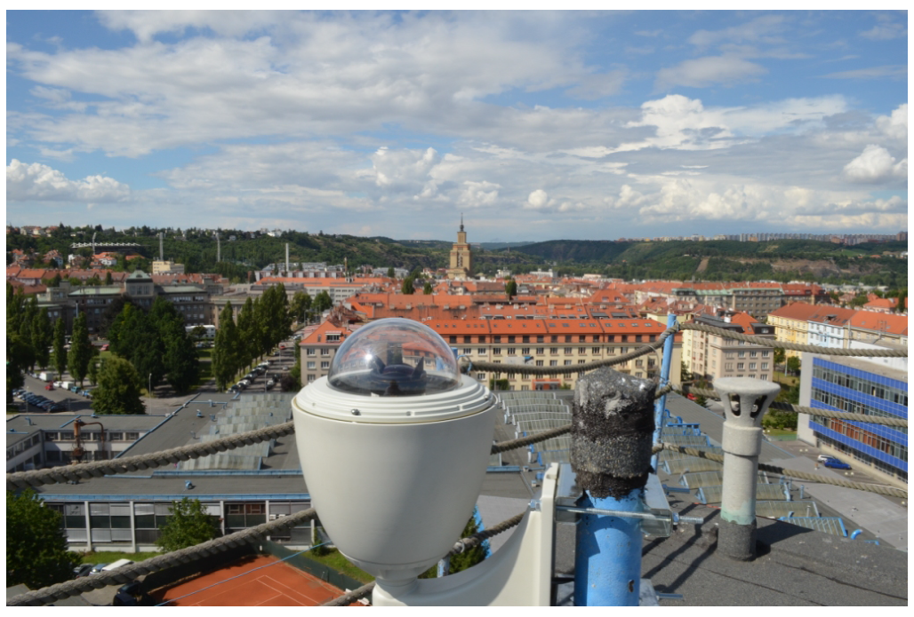
Currently, the WILLIAM system operates in Jarošov nad Nežárkou (South Bohemia, Czechia, GPS ${49.185}^{\circ }$N, ${15.072}^{\circ }$E). This station is equipped with a NIKON D5100 camera with a CMOS 23.5 × 15.6 mm sensor, which provides a maximal resolution of 3264 × 4928 pixels and 24 bit color depth. An all-sky scenery display with a field-of-view equal to ${154}^{\circ }$ (${180}^{\circ }$ with a Nikon full-frame camera) is provided by a Sigma 10 mm diagonal fish-eye lens. The standard setting for daytime image acquisition is f/2.8, exposure value 1/2000 s, and ISO 100. Images are automatically saved on the remote server in the RAW data format.

The camera with supporting electronics is enclosed in a weather-proof housing box, allowing observation throughout the year, irrespective of the weather conditions. The housing was also tested in the climate chamber.

The WILLIAM system captures a huge amount of image data each year. One set of data has been manually labeled and made available in the WILLIAM Meteo Database (WMD (http://william.multimediatech.cz/meteorology-camera/william-meteo-database/)). WMD contains 2044 daytime images with labeled cloud phenomena. The images have been preselected to cover a variety of conditions during a different daytime and during the year. The clouds in the images have been classified into ten fundamental cloud classes, according to the WMO (World Meteorological Organization [19]) classification. No division into cloud species and varieties has been specified. The cloud cover data for various cloud levels from the ALADIN (Aire Limitée, Adaptation Dynamique, Development International [20]) numerical weather model has also been exploited for the classification. The cloud types have been split into four cloud groups, also according to the WMO cloud level classification system. These cloud groups have been customized for the data from the WILLIAM system. Each cloud group incorporates the clouds with similar characteristics and appearance on all-sky images. The cloud groups, their color labels used in the diagrams, and their qualitative descriptors are listed in

Table 1. Used WMO (World Meteorological Organization) cloud classes.

Group No.	Cloud Types	Qualitative Descriptors	Color Labels
1	Cirrus (CIR), Cirrocumulus (CIR-CUM),	high-level clouds	cyan
	Cirrostratus (CIR-STR), Altocumulus (ALT-CUM) *
2	Cumulus (CUM), Stratocumulus (STR-CUM),	low-level	red
	Altocumulus (ALT-CUM)	cumulus type clouds
	Cumulonimbus (CUM-NIMB) **
3	Stratus (STR), Altostratus (ALT-STR),	rain clouds	green
	Nimbostratus (NIMB-STR), Cumulonimbus (CUM-NIMB)
4	Clear Sky	-	blue

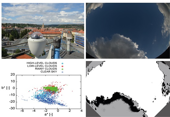
* Sparse altocumulus clouds located at a such altitude that are indistinguishable on the image from the high-level clouds; ** Possible cumulonimbus cloud, which is far from the center of the image and is indistinguishable from other cumulus-type clouds.

. The WMD contains 492 images with high-level clouds, 833 images with low-level cumuli-type clouds, 793 images with rain clouds, and 1411 images with clear sky. The cloud groups serve as the primary classification categories and are based on the WMO system. The division into the cloud groups also offers minimization of the systematic classification bias. For further consistent color processing results, all RAW all-sky images have been preserved in TIFF format and have been white-balanced to noon-day light of 6000 Kelvin.

3. Methods and Algorithms

Let the input all-sky color RGB (Red, Green, Blue) image be represented as a set of slices $I_{RGB}(i,j,c)$, where the indices are used for spatial and color dimensions. Indices $i=1,\cdots ,W$, $j=1,\cdots ,H$, and $c=1,\cdots ,N_c$. Symbols $W,H$ are used for the width and the height of the image. $N_c$ is the number of color channels that are used. Based on the results presented in Blažek [16], we selected the two most suitable color-spaces for cloud segmentation, CIE ${\mathrm{La}}^{*}{\mathrm{b}}^{*}$ [21] and CIE XYZ [22]. These two color-spaces offer the greatest sensitivity in the chromaticity diagram for separating the cloud types from the blue sky tone. Applying the equations from [23] to the input, $I_{RGB}$ can be transformed into a new color basis as:

$$\begin{array}{c}\hfill I_{RGB}\to I_{XYZ}\end{array}$$

(1)

$$\begin{array}{c}\hfill I_{RGB}\to I_{L{a}^{*}{b}^{*}}\end{array}$$

(2)

The RGB to CIE XYZ transformation can be described as:

$$\left[XYZ\right]=\left[RGB\right]M$$

(3)

Assuming the CIE standard illuminant D65, the conversion matrix M [24] may be represented as:

$$M=\left[\begin{array}{ccc}0.4124& 0.3576& 0.1805\\ 0.2126& 0.7152& 0.7220\\ 0.1933& 0.1192& 0.9505\end{array}\right]$$

(4)

To obtain the chromaticity x, y, z values from the CIE XYZ space, the tristimulus X, Y, Z values have to be normalized as:

$$\begin{array}{c}\hfill x=\frac{X}{X+Y+Z},y=\frac{Y}{X+Y+Z},z=\frac{Z}{X+Y+Z}\end{array}$$

(5)

However, $x+y+z=1$, and therefore, only two chromaticity components are necessary for defining the chrominance. Subsequently, the RGB to CIE ${\mathrm{La}}^{*}{\mathrm{b}}^{*}$ transformation builds on the previous RGB to CIE XYZ transformation and is defined as:

$$L=116f\left(\frac{Y}{Y_n}-16\right),$$

(6)

$$a^{*}=500\left[f\left(\frac{X}{X_n}\right)-f\left(\frac{Y}{Y_n}\right)\right],$$

(7)

$$b^{*}=500\left[f\left(\frac{Y}{Y_n}\right)-f\left(\frac{Z}{Z_n}\right)\right],$$

(8)

for:

$$\begin{array}{c}\hfill f\left(x\right)=\left\{\begin{array}{cc}{x}^{\frac{1}{3}}\hfill & x\ge 0.008856\hfill \\ 7.787.x+\frac{16}{116},\hfill & x\le 0.008856\hfill \end{array}\right.,\end{array}$$

(9)

and for $X_n=95.04$, $Y_n=100.00$, and $Z_n=108.88$. For the purpose of this work, $a^{*}$, $b^{*}$, and x, z are chromaticity channels and L, Y are luminosity channels. The luminosity channels are used only for equalizing the sensor illumination, and they can be omitted for the segmentation method. Reducing the color-space dimension to a set of two independent chromaticity components leads to more effective convergence.

The proposed segmentation method was based on a heuristic approach derived from the modified k-means++ algorithm [25]. The maximum number of different cloud classes in the analyzed image is $K_{max}$. Typically, the maximum number can be set to $K_{max}\le 4$ (see Table 1), plus other classes in reserve to cover other disturbing details in the image, e.g., parts of buildings, planes, and other artificial objects. The cost function for the analysis is set to:

$${\mathsf{\Delta }}_s^{\varrho }=\frac{1}{WH{N}_c}\sqrt{\sum _{c=2}^{N_c}\sum _{i=1}^W\sum _{j=1}^H\left|\right|\mathrm{I}(\mathrm{i},\mathrm{j},\mathrm{c})-{\mu }_{s-1}^{\varrho }\left(c\right){\left|\right|}^2},$$

(10)

where s is the index of the current iteration and $\varrho =1,\cdots ,K_{max}$ is used for the index of the cloud group. $I(i,j,c)$ are pixels of the image in the CIE ${\mathrm{L}}^{*}{\mathrm{a}}^{*}{\mathrm{b}}^{*}$ ($I_{Lab}$) and CIE XYZ ($I_{XYZ}$) representation, and two chromaticity channels were used. The luminosity channel $I(i,j,1)$ was omitted for the cloud groups separation. The aim was to minimize the Euclidean distance of the image pixel color values to the initial centroids ${\mu }_{s-1}\left(c\right)$. The centroids were derived each time in the previous iteration $s-1$. The initial approximation of the centroid position can be set as:

$${\mu }_0^{\varrho }\left(c\right)=\mathrm{rand}\{\min \left(I(i,j,c)\right),\max \left(I(i,j,c)\right)\}c=1,2,\forall i,j.$$

(11)

The value of criterion function ${\mathsf{\Delta }}_s^{\varrho }$ was calculated in each step. The distance between pixel $I(i,j,c)$ and the center of the cloud centroid is expressed as:

$$D^{\varrho }(i,j)=\frac{1}{N_c}\sqrt{\sum _{c=1}^{N_c}{(I(i,j,c)-{\mu }_{s-1}^{\varrho })}^2}.$$

(12)

Pixels with the distance-satisfying condition:

$$D^{\varrho }(i,j)\le \epsilon {\mathsf{\Delta }}_s^{\varrho }$$

(13)

are marked as potentially classified as a single cloud class $\varrho$. $\epsilon >0$ is a sensitivity parameter of the convergence of the method. The segmentation process is completed when each pixel can be distinguished as a single cloud group (see Table 1) in the chromaticity color-space, or when the maximum number of iterations has been taken. The input image can also contain unwanted artificial objects. To remove these areas of the image, a special pixel color mask is applied to the images. These objects can be simply masked out as an additional color cluster.

4. Results and Discussion

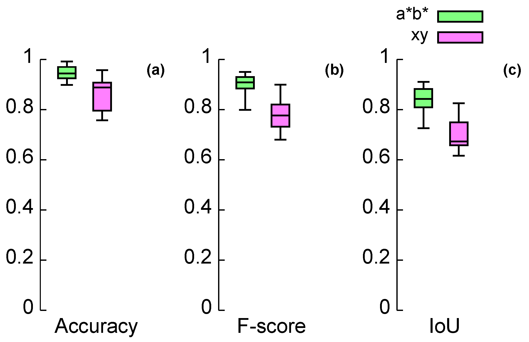
Since all of the images have been classified and evaluated, the next step was an investigation of the segmentation accuracy of the proposed method. Two different color-spaces were chosen for the comparison: CIE ${\mathrm{L}}^{*}{\mathrm{a}}^{*}{\mathrm{b}}^{*}$ and the CIE XYZ space.

Figure 2 presents the segmentation of the phenomena in the $a^{*}$, $b^{*}$ color channels. Figure 3 presents a similar segmentation in the x, z channels. Firstly, a visual inspection of the segmentation accuracy was done for all images in the WMD database. In general, the separation of the clouds and the clear sky segments was more precise in the $a^{*}$, $b^{*}$ channels than in the x, z channels. In particular, parts of low-level clouds were frequently separated into one of the produced segments together with a clear sky in the x, z channels (see the light-gray segment in Figure 3). By contrast, the clear sky and the clouds were very precisely separated into stand-alone segments in the $a^{*}$, $b^{*}$ channels. We supported these observations by several segmentation accuracy metrics such as pixel accuracy, the F-score, also known as the Dice coefficient, and IoU (Intersection over Union), also known as the Jaccard coefficient.

From the WMD database, there were annotated (classified) cloud groups for each image. In addition, each cloud group had its own, manually labeled, ground truth segments. Ground truth represents pixel areas that contained a particular cloud group or artificial objects and edges in an image. If an image contained several cloud groups, each group in the image had its own ground truth. The artificial objects also had their own ground truth pixel area. The k-means++ method produced several segments. They had to be manually assigned to one of the cloud groups or artificial objects. One cloud group could comprise several generated segments, which were joined together. Subsequently, the pixels within the generated and classified segment could be compared with the pixels of the equally classified ground truth. The number of different ground truth segments in the image was equal to $K_{max}$. The number of generated and classified segments (pixel areas, which belonged to the cloud groups or artificial objects) had to be also equal to $K_{max}$. Therefore, the score of each metric for one image had to be calculated separately for $K_{max}$ cases and then averaged over $K_{max}$. Assume a binary representation, where pixels are either zero if they do not belong to the selected area (segment) or one if they belong to the selected area (segment). Let there be a pixel-wise task, where pixels within a generated segment are evaluated against pixels of a ground truth segment as TP (True Positive), TN (True Negative), FP (False Positive), and FN (False Negative). For one image, assume $K_{max}$ such pixel-wise tasks. Then, the pixel accuracy metric, F-score, and IoU, respectively, are defined as:

$$\mathrm{Accuracy}=\frac{1}{K_{max}}\sum _{i=1}^{K_{max}}\frac{T{P}_i+T{N}_i}{T{P}_i+T{N}_i+F{P}_i+F{N}_i},$$

(14)

$$\mathrm{F-score}=\frac{1}{K_{max}}\sum _{i=1}^{K_{max}}\frac{2\times T{P}_i}{2\times T{P}_i+F{P}_i+F{N}_i},$$

(15)

$$\mathrm{IoU}=\frac{1}{K_{max}}\sum _{i=1}^{K_{max}}\frac{T{P}_i}{T{P}_i+F{P}_i+F{N}_i}.$$

(16)

Figure 4 presents the results of the metrics for our segmented all-sky images. All three metrics showed higher values and lower variation for the cloud group segmentation in the $a^{*}$, $b^{*}$ color channels than in the x, z color channels. This, therefore, indicated higher segmentation accuracy of the cloud groups within the $a^{*}$, $b^{*}$ channels.

After the visual inspection combined with the results of the introduced objective metrics, we could conclude that the $a^{*}$, $b^{*}$ color channels were more suitable than the x, z color channels for color-based segmentation of all-sky images. Due to the inaccurate separation in the x, z channels, an additional bias in the color values of the cloud segments was anticipated.

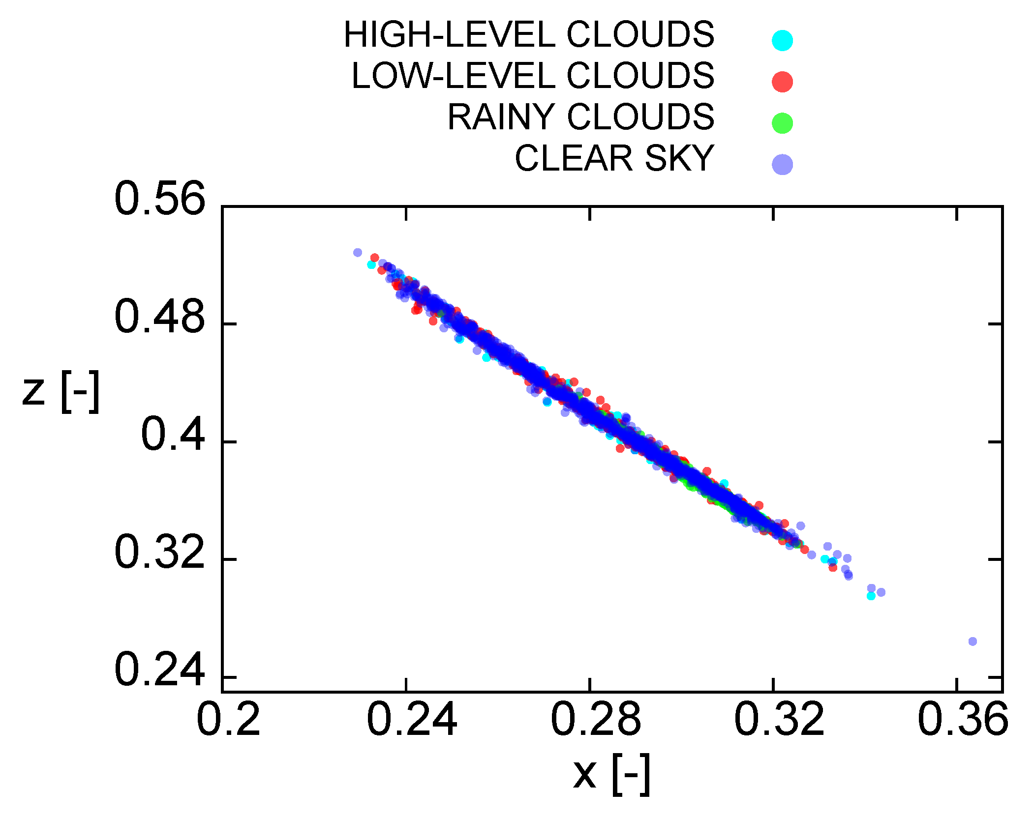
For the investigation of cloud groups color features, it was convenient to extract the color values (features) from the generated segments. Subsequently, the investigation of the distribution of these cloud-segment color features was carried out within the color-spaces that were introduced. The original images were again transformed into the CIE XYZ and CIE ${\mathrm{La}}^{*}{\mathrm{b}}^{*}$ color-spaces. During the previous process of segmentation accuracy evaluation, k-means++ generated segments could be merged and classified as one of the cloud groups. The pixel areas in the again transformed images, which belonged to the classified segments, were extracted. For such segments, the mean values of each color-space channel were calculated. Due to the repeated color transformations, we were also able to extract the luminosity channels Y and L of the cloud group segments. It was possible to compare the features of the cloud-group segments in the chrominance and luminosity channels, even though the luminosity channels were previously omitted from the segmentation process. For the investigation of cloud-segment color features, we exploited the diagrams of the selected color-space channels plotted against each other (Figure 5, Figure 6 and Figure 7). To clarify, each data point in the following diagrams represents a segment classified into one of four main cloud groups. 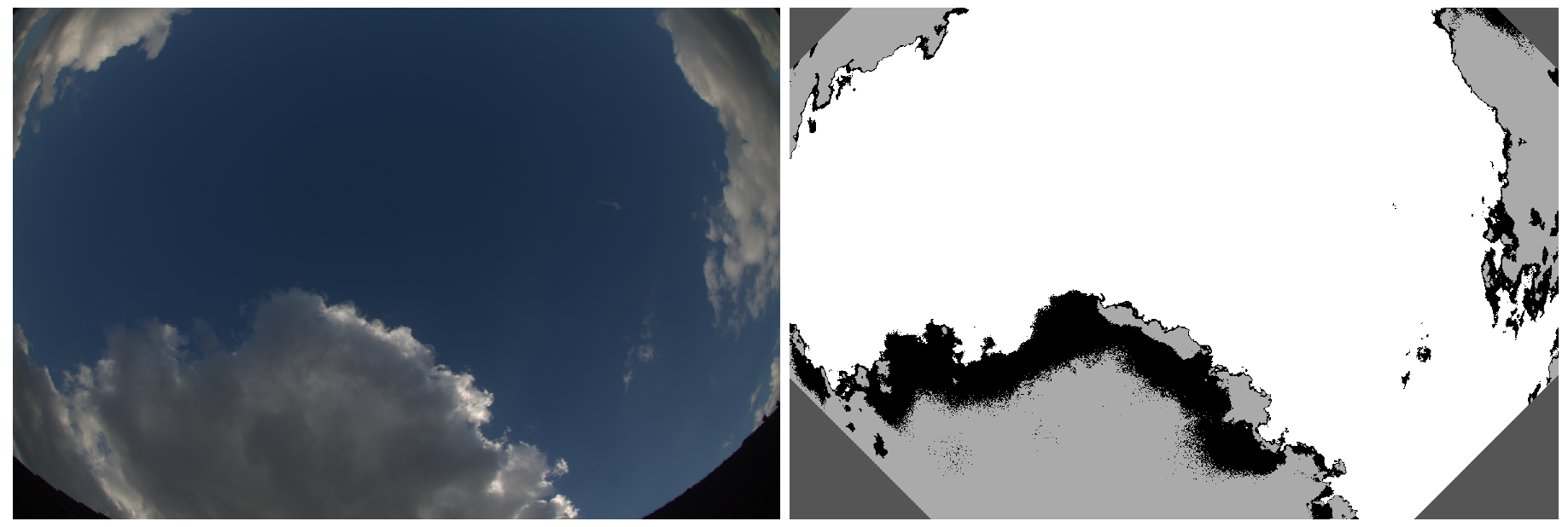For example, Figure 2 represents two segments joined and classified as low-level clouds and one segment of the clear sky. However, due to the inaccurate segmentation, Figure 3 represents one classified segment of low-level clouds and two joined and classified segments of clear sky. The segments of masked out artificial objects were generally omitted from the color evaluation.

In this paper, we present and discuss only those color diagrams with the most promising and most significant results. The most exploited color diagrams that we introduce here mainly show the color components of the CIE ${\mathrm{L}}^{*}{\mathrm{a}}^{*}{\mathrm{b}}^{*}$ color-space. Only to support the exclusion of the CIE XYZ color-space from the cloud-segment color analysis, we also present a color diagram of the x, z components in which the segmentation proceeded. As expected, the previous segmentation inaccuracy significantly influenced the distribution of our segments within the x, z diagram (Figure 5). There was massive overlapping of the cloud segment data points by the clear sky data points (blue). Due to this overlapping distribution, it was not possible to perform any further statistical analysis or to make any other use of the data. In general, we considered that the CIE XYZ color-space was unsuitable for cloud color segmentation of all-sky images.

Diagrams L, $b^{*}$ (Figure 6) and $a^{*}$, $b^{*}$ (Figure 7) offered much more promising data distributions. The inaccurate segmentation and cloud separation in the image data taken close to sunrise or sundown were already observed during the classification process. This inaccuracy was imprinted in the diagrams. Although we segmented the data only in the chrominance channels, the low-light conditions affected the segmentation results. The F-score lower extreme was close to 0.79. This conclusion was confirmed by the L, $b^{*}$ diagram (Figure 6). The points representing clear sky (blue) with low L values were closer to the points representing rain clouds (green). However, with average light L values, the clear sky points were completely separated from the rainy points. The highly solar irradiated scene also significantly affected the color values of the segments. This could be observed in the L, $b^{*}$ diagram, in which the points of all groups with L values greater than 80 significantly overlapped each other.

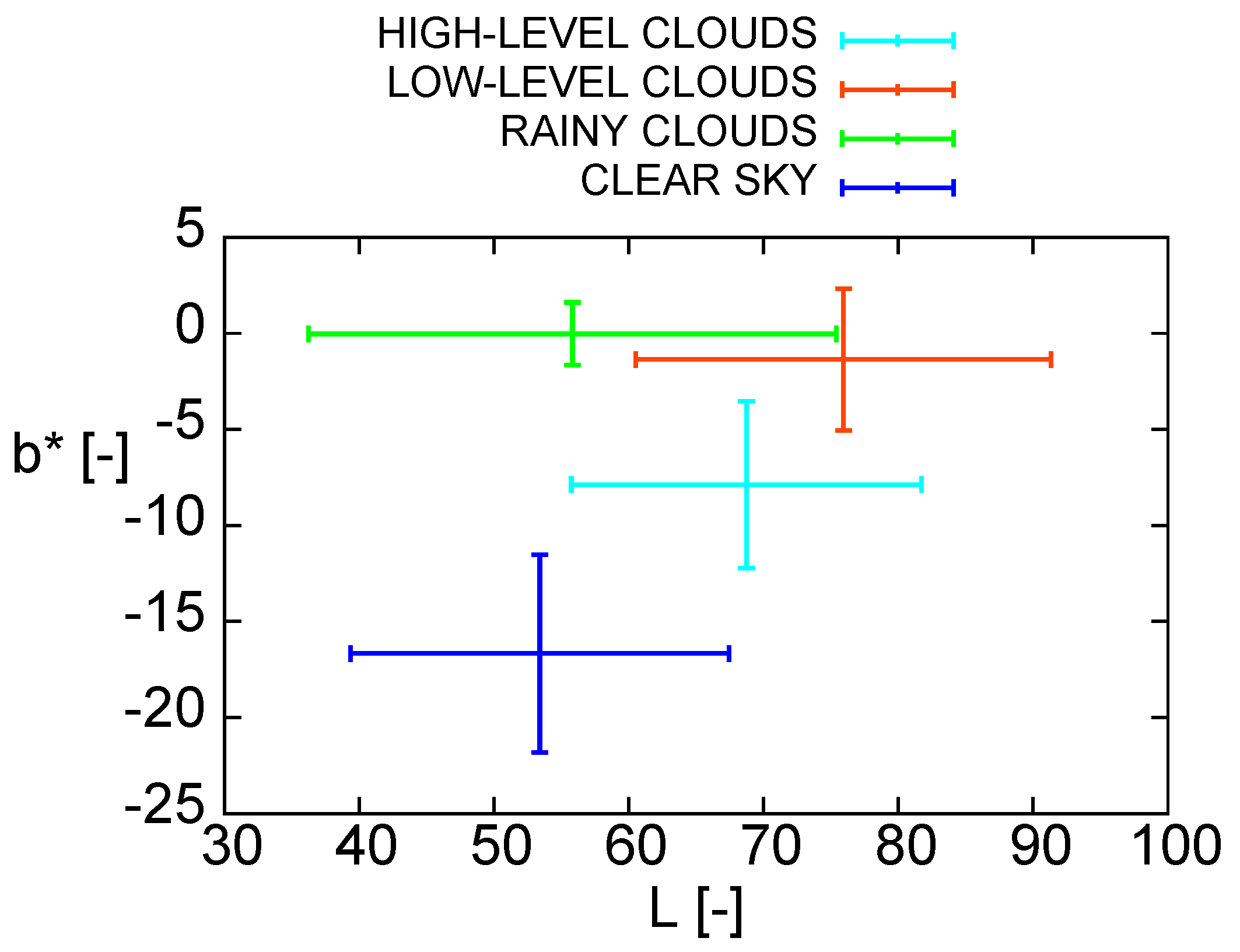
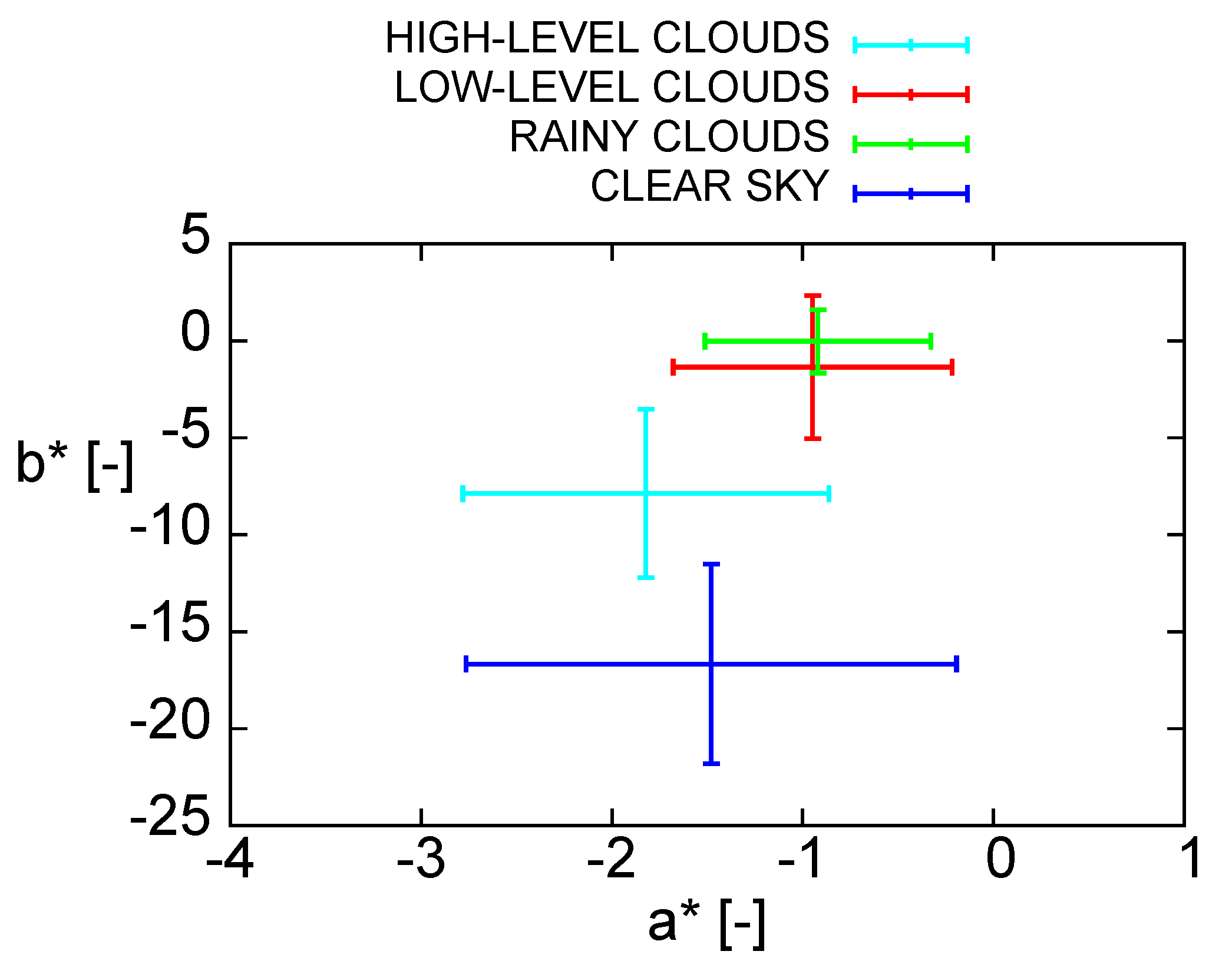
Despite the frequent overlapping caused by the significant number of segments and the segmentation bias, however, it was apparent that each of the cloud groups formed a cluster within the diagram. If we evaluated each cloud group separately and computed the mean value with the standard deviation for each group, we obtained the diagram in Figure 8, in which these centroids were clearly separated. The separation between the cloud group data distribution was measured by the Bhattacharyya coefficient [26,27], which approximates the relative closeness between the distributions. BC values are equal to one when two data distribution are identical and equal to zero when two data distributions have no intersection. The Bhattacharyya coefficient ($BC$) is defined as:

$$BC=1/exp\left(B{D}_{1,2}\right),$$

(17)

where $B{D}_{1,2}$ represents the Bhattacharyya distance between two multivariate distributions with their mean values ${\mathit{\mu }}_1$, ${\mathit{\mu }}_2$ and covariance matrices ${\mathsf{\Sigma }}_1$, ${\mathsf{\Sigma }}_2$. The Bhattacharyya distance is expressed as:

$$B{D}_{1,2}=\frac{1}{8}{\left({\mathit{\mu }}_1-{\mathit{\mu }}_2\right)}^{\mathbf{T}}{\left(\frac{{\mathsf{\Sigma }}_1+{\mathsf{\Sigma }}_2}{2}\right)}^{-1}\left({\mathit{\mu }}_1-{\mathit{\mu }}_2\right)\frac{1}{2}ln\left(\frac{det\left(\frac{{\mathsf{\Sigma }}_1+{\mathsf{\Sigma }}_2}{2}\right)}{\sqrt{det{\mathsf{\Sigma }}_{1}det{\mathsf{\Sigma }}_2}}\right).$$

(18)

Especially, rain cloud (green) and clear sky (blue) segments or low-level cumulus-type clouds (red) and clear sky (blue) segments reported low values of the $BC$, 0.05 and 0.13, respectively, and therefore, a high separation between them within the L, $b^{*}$ channels. All values of the $BC$ for the cloud groups within the L, $b^{*}$ channels are listed in

Table 2. The Bhattacharyya coefficient ($BC$) for the possibility of the cloud groups’ separation in $\mathrm{L},{\mathrm{b}}^{*}$ channels. The coefficient is normalized between values of zero and one, supposing the high and low possibility of separation, respectively.

Cloud Group No.	1	2	3	4
and Color Label	(Cyan)	(Red)	(Green)	(Blue)
1 (cyan)	1	0.66	0.28	0.56
2 (red)	0.66	1	0.63	0.13
3 (green)	0.28	0.63	1	0.05
4 (blue)	0.56	0.13	0.05	1

. The values of BC in the table indicated that the cloud groups’ data distributions were non-identical in the L, $b^{*}$ space. It was, therefore, possible to exploit the cloud groups in this space as classification classes for a classification task. However, due to the frequent overlapping of some data points, the classification task only in the L, $b^{*}$ space may be problematic. It was apparent that even if the luminosity was omitted from the segmentation process, the illumination conditions of a taken scene affected the color values of the cloud segments. The color of the cloud groups varied during the day. For future work, it is substantial to incorporate some machine learning techniques into the process of cloud classification development. Additional parameters, which would take into consideration the illumination of the scene and the variation of the cloud color during the day, have to be introduced.

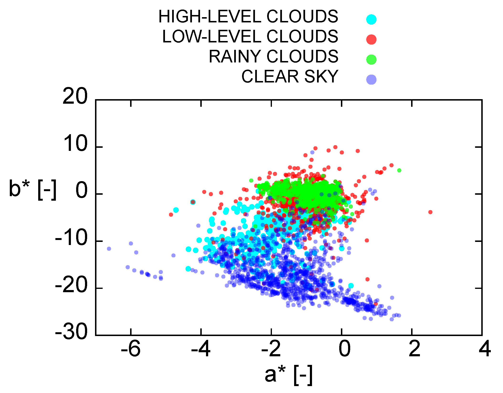
The next color diagram (Figure 7) of component $a^{*}$ versus $b^{*}$ also provided interesting results. In this diagram, the rain cloud segment points (green) had similar color features to those of the low-level cumulus-type clouds (red). This supported similar claims in [16]. Similarly, the high-level clouds (magenta) were also located close to the points of clear sky (blue).

Despite the overlapping of some points, it was apparent that the low-level clouds (red) and the rain clouds (green) formed their own clusters within these channels. These clusters were clearly separated from the high-level clouds and the clear sky points, which formed clusters of their own. We therefore decided to calculate the mean value of these clusters with the standard deviation and to plot these centroids in the new color diagram (Figure 9). The separation of the centroids of the cloud groups confirmed the formation of the cloud-group clusters within the $a^{*}$, $b^{*}$ space. For the inspection of the separation between the cloud groups within the $a^{*}$, $b^{*}$ channels, the Bhattacharyya coefficient was again calculated. The values of the coefficient are listed in

Table 3. The Bhattacharyya coefficient ($BC$) for the possibility of cloud groups’ separation in $\mathrm{a},{\mathrm{b}}^{*}$ channels. The coefficient is normalized between values of zero and one, supposing the high and low possibility of separation, respectively.

Cloud Group No.	1	2	3	4
and Color Label	(Cyan)	(Red)	(Green)	(Blue)
1 (cyan)	1	0.67	0.35	0.58
2 (red)	0.67	1	0.78	0.11
3 (green)	0.35	0.78	1	0.03
4 (blue)	0.58	0.11	0.03	1

. In the $a^{*}$, $b^{*}$ space, BC also indicated that the cloud group distributions were non-identical. However, rain clouds and low-level clouds were more closely related in this space (higher BC). It was more problematic to differentiate between them. The differentiation of the cloud groups in this space was still possible, and this space was valuable for the possible classification task. In the future, it would be necessary to incorporate all the cloud color features from the ${\mathrm{La}}^{*}{\mathrm{b}}^{*}$ color-spaces and also an investigation of cloud color variations during the day. In addition, for the cloud types’ classification, exploitation of some machine learning techniques, especially the soft-classification methods, would be beneficial.

In general, the results confirmed that cloud detection on all-sky images could be performed by color segmentation within the CIE ${\mathrm{L}}^{*},{\mathrm{a}}^{*},{\mathrm{b}}^{*}$ color-space. In addition, the color diagrams explored the diverse color features of the clouds merged into the defined groups. It was therefore possible to distinguish a variety of clouds on all-sky images according to their color features. Due to the sufficient quantity of the classified data from the WMD database, the cloud color features could be exploited as training data for developing a new automatic cloud classification algorithm. The separation of the cloud groups within the color diagrams implied that a properly designed algorithm, based for example on machine learning techniques or on neural networks, would automatically classify the clouds on all-sky images, after k-means++ preprocessing and after extracting the color-features. This cloud classification algorithm could then be extended for detecting rain clouds or for predicting the probability of rain. The proposed method based on k-means++ and other required image processing techniques could easily be optimized, and the algorithm could even operate in real-time on all-sky imaging systems. Color-based classification of clouds in all-sky images could therefore be a promising field of investigation for research groups with their own ground-based all-sky imaging system.

5. Conclusions

This paper presented an evaluation of the k-means++ cloud color-based segmentation algorithm based on all-sky image data from the WILLIAM ground-based whole sky imaging system. The algorithm was tested on 2044 cloud-classified all-sky images, which had been consolidated into the WMD database.

The evaluation proceeded in two color-spaces, CIE ${\mathrm{L}}^{*},{\mathrm{a}}^{*},{\mathrm{b}}^{*}$ and CIE XYZ, the segmentation accuracy of which was compared. For further cloud color analysis, the clouds within the segments were classified into four distinct cloud groups. The color features of these classified segments were also investigated. The overall results indicated that the CIE XYZ color-space was unsuitable for segmentation of all-sky images. However, segmentation in CIE ${\mathrm{L}}^{*},{\mathrm{a}}^{*},{\mathrm{b}}^{*}$ offered better accuracy. Suitable objective metrics were used for assessing the segmentation accuracy. In addition, the color values of the cloud-group segments were promisingly distributed and formed their own separate clusters within this color-space. The cluster separation of the rain cloud types was especially important. All-sky image color segmentation and cloud-type color-feature clustering therefore have tremendous potential for the development of color-based cloud detection and classification algorithms. The proposed method based on k-means++ color segmentation of all-sky image data could therefore be exploited in the future for color-based weather and rainfall prediction based on automatic all-sky systems and could be used for further cloud color-based research.

References

1. Neshat, M.; Ahmadi, M. Recognising the kind of cloud using a new fuzzy knowledge-based system. Int. J. Reason. Based Intell. Syst. 2016, 8, 168–180. [Google Scholar] [CrossRef]
2. Sun, R.; Yu, S.; Zhao, C.; Zhang, W. Algorithms for surveying and cataloguing space debris utilizing a wide field of view telescope. Publ. Astron. Soc. Jpn. 2019, 71, 67. [Google Scholar] [CrossRef]
3. Dev, S.; Nautiyal, A.; Lee, Y.H.; Winkler, S. CloudSegNet: A Deep Network for Nychthemeron Cloud Image Segmentation. IEEE Geosci. Remote Sens. Lett. 2019, 16, 1814–1818. [Google Scholar] [CrossRef] [Green Version]
4. Liu, S.; Zhang, L.; Zhang, Z.; Wang, C.; Xiao, B. Automatic Cloud Detection for All-Sky Images Using Superpixel Segmentation. IEEE Geosci. Remote Sens. Lett. 2015, 12, 354–358. [Google Scholar] [CrossRef]
5. Dev, S.; Savoy, F.M.; Lee, Y.H.; Winkler, S. High-dynamic-range imaging for cloud segmentation. Atmos. Meas. Tech. 2018, 11, 2041–2049. [Google Scholar] [CrossRef]
6. Dev, S.; Lee, Y.H.; Winkler, S. Color-Based Segmentation of Sky/Cloud Images From Ground-Based Cameras. IEEE J. Sel. Top. Appl. Earth Obs. Remote Sens. 2017, 10, 231–242. [Google Scholar] [CrossRef]
7. Taravat, A.; Del Frate, F.; Cornaro, C.; Vergari, S. Neural Networks and Support Vector Machine Algorithms for Automatic Cloud Classification of Whole-Sky Ground-Based Images. IEEE Geosci. Remote Sens. Lett. 2015, 12, 666–670. [Google Scholar] [CrossRef]
8. Ye, L.; Cao, Z.; Xiao, Y.; Yang, Z. Supervised Fine-Grained Cloud Detection and Recognition in Whole-Sky Images. IEEE Trans. Geosci. Remote Sens. 2019, 57, 7972–7985. [Google Scholar] [CrossRef]
9. Cheng, H.Y.; Lin, C.L. Cloud detection in all-sky images via multi-scale neighborhood features and multiple supervised learning techniques. Atmos. Meas. Tech. 2017, 10, 199–208. [Google Scholar] [CrossRef] [Green Version]
10. Zhuo, W.; Cao, Z.; Xiao, Y. Cloud Classification of Ground-Based Images Using Texture–Structure Features. J. Atmos. Ocean. Technol. 2014, 31, 79–92. [Google Scholar] [CrossRef]
11. Oikonomou, S.; Kazantzidis, A.; Economou, G.; Fotopoulos, S. A local binary pattern classification approach for cloud types derived from all-sky imagers. Int. J. Remote Sens. 2019, 40, 2667–2682. [Google Scholar] [CrossRef]
12. Dev, S.; Savoy, F.M.; Lee, Y.H.; Winkler, S. Rough-Set-Based Color Channel Selection. IEEE Geosci. Remote Sens. Lett. 2017, 14, 52–56. [Google Scholar] [CrossRef] [Green Version]
13. Heinle, A.; Macke, A.; Srivastav, A. Automatic cloud classification of whole sky images. Atmos. Meas. Tech. 2010, 3, 557–567. [Google Scholar] [CrossRef] [Green Version]
14. Kazantzidis, A.; Tzoumanikas, P.; Bais, A.F.; Fotopoulos, S.; Economou, G. Cloud detection and classification with the use of whole-sky ground-based images. Atmos. Res. 2012, 113, 80–88. [Google Scholar] [CrossRef]
15. Long, C.N.; Sabburg, J.M.; Calbó, J.; Pagès, D. Retrieving Cloud Characteristics from Ground-Based Daytime Color All-Sky Images. J. Atmos. Ocean. Technol. 2006, 23, 633–652. [Google Scholar] [CrossRef] [Green Version]
16. Blazek, M.; Pata, P. Colour transformations and K-means segmentation for automatic cloud detection. Meteorol. Z. 2015, 24, 503–509. [Google Scholar] [CrossRef]
17. Janout, P.; Blažek, M.; Páta, P. New generation of meteorology cameras. In Photonics, Devices, and Systems VII; Fliegel, K., Páta, P., Eds.; International Society for Optics and Photonics, SPIE: Bellingham, WA, USA, 2017; Volume 10603, pp. 312–318. [Google Scholar] [CrossRef]
18. Janout, P.; Páta, P.; Bednář, J.; Anisimova, E.; Blažek, M.; Skala, P. Stellar objects identification using wide-field camera. In Photonics, Devices, and Systems VI; Tománek, P., Senderáková, D., Páta, P., Eds.; SPIE: Bellingham, WA, USA, 2015; Volume 9450, pp. 380–388. [Google Scholar] [CrossRef]
19. World Meteorological Organization. International Cloud Atlas; WMO [publications]; no. 407; Secretariat of the World Meteorological Organization: Geneva, Switzerland, 1975. [Google Scholar]
20. Wang, Y.; Bellus, M.; Wittmann, C.; Steinheimer, M.; Weidle, F.; Kann, A.; Ivatek-Šahdan, S.; Tian, W.; Ma, X.; Tascu, S.; et al. The Central European limited-area ensemble forecasting system: ALADIN-LAEF. Q. J. R. Meteorol. Soc. 2011, 137, 483–502. [Google Scholar] [CrossRef]
21. McLaren, K. XIII-The Development of the CIE 1976 (L* a* b*) Uniform Colour Space and Colour-difference Formula. J. Soc. Dye. Colour. 2008, 92, 338–341. [Google Scholar] [CrossRef]
22. Smith, T.; Guild, J. The C.I.E. colorimetric standards and their use. Trans. Opt. Soc. 1931, 33, 73–134. [Google Scholar] [CrossRef]
23. Meshta, L.K. Control of Colour Imaging Systems: Analysis and Design; CRC Press: Boca Raton, FL, USA, 2009; pp. 628–641. [Google Scholar]
24. Giorgianni, E.J.; Madden, T.E. Digital Color Management: Encoding Solutions; Addison-Wesley Longman Publishing Co., Inc.: Boston, MA, USA, 1998. [Google Scholar]
25. Arthur, D.; Vassilvitskii, S. K-means++: The advantages of careful seeding. In Proceedings of the 18th Annual ACM-SIAM Symposium on Discrete Algorithms, New Orleans, LA, USA, 7–9 January 2007. [Google Scholar]
26. Bhattacharyya, A. On a measure of divergence between two statistical populations defined by their probability distributions. Bull. Calcutta Math. Soc. 1943, 35, 99–109. [Google Scholar]
27. Koutroumbas, K.; Theodoridis, S. Pattern Recognition; Elsevier: Amsterdam, The Netherlands, 2008. [Google Scholar]
Figure 1. The WILLIAM all-sky ground-based imaging and monitoring system.
Remotesensing 12 01902 g001
Figure 2. An example of an all-sky image from the WILLIAM system (left), showing cumulus-type clouds and the results of k-means++ color-based segmentation (right). The image was transformed into a * , b * channels and was segmented into four clusters. One cluster represents the masked static objects at the edges of the image. The next white cluster was classified as Clear Sky (Group 4 in Table 1). The remaining black and grey cluster was classified as Cumulus Group 2. The solar zenith angle of the image is 65.31 .
Remotesensing 12 01902 g002
Figure 3. The same example of an all-sky image from the WILLIAM system (left) as was presented in Figure 2 and the results of k-means++ color-based segmentation (right). The image was transformed into x, z channels and was also segmented into four clusters. In this case, the white and grey clusters were classified as Clear Sky (Group 4), and the one black cluster was classified as Cumulus Group 2. The solar zenith angle of the image is 65.31 .
Remotesensing 12 01902 g003
Figure 4. The box-plot diagrams of selected objective metrics. The metrics represent the segmentation accuracy of the segmented cloud groups within the a * , b * and x, z color channels against the ground truth. The first diagram (a) represents the pixel accuracy metric; the second diagram (b) expresses the F-score; the third diagram (c) represents the IoU. The whiskers represent extreme values; the top and bottom edges of the boxes indicate the 25th and 75th percentiles; the central line within the boxes corresponds to the median. Values of the metrics are normalized between zero and one.
Remotesensing 12 01902 g004
Figure 5. Cloud group color diagram for components x, z obtained from the data in the database. Each point represents the segmented cluster average value classified into four cloud groups.
Remotesensing 12 01902 g005
Figure 6. Cloud group color diagram for components L, b * obtained from the data in the database. Each point represents the segmented cluster average value classified into four cloud groups.
Remotesensing 12 01902 g006
Figure 7. Cloud group color diagram for components a * , b * obtained from the data in the database. Each point represents the segmented cluster average value classified into four cloud groups.
Remotesensing 12 01902 g007
Figure 8. Centroids calculated from data in Figure 6, representing the mean values and the standard deviation for each cloud group.
Remotesensing 12 01902 g008
Figure 9. Centroids calculated from the data in Figure 7, representing the mean values and the standard deviation for each cloud group.
Remotesensing 12 01902 g009