Article

GIS Data as a Valuable Source of Information for Increasing Resolution of the WRF Model for Warsaw

by
Jolanta Siewert
* and
Krzysztof Kroszczynski
Institute of Geospatial Engineering and Geodesy, Faculty of Civil Engineering and Geodesy, Military University of Technology, 2 Gen. S. Kaliskiego St., 00-908 Warsaw, Poland
*
Author to whom correspondence should be addressed.
Remote Sens. 2020, 12(11), 1881; https://doi.org/10.3390/rs12111881
Submission received: 5 May 2020 / Revised: 7 June 2020 / Accepted: 8 June 2020 / Published: 10 June 2020

Abstract

:
The Weather Research and Forecasting (WRF) model is commonly associated with meteorological data, but its algorithms may also use geographical data. The objective of this paper is to evaluate the impact of the high resolution CORINE Land Cover (CLC) data and the SRTM topography on the estimation accuracy of the weather model parameters in the WRF microscale simulations (200 × 200 m) for Warsaw. In the presented studies, the authors propose their own method of attaching the CLC data to the WRF microscale modeling for the CLC border areas, where first calculational domains reach beyond areas of CLC coverage. As a part of the research, the adaptation of the proposed method was examined by the assessment of the WRF microscale modeling simulations for Warsaw. The modified IGBP MODIS land use/land cover (LULC) and USGS GMTED2010 terrain elevation geographical data (30 arc seconds) was applied for the WRF simulations as default. As higher resolution geographical data (100 m), the LULC from CORINE Land Cover (CLC) 2018 data, and the SRTM topography were adopted. In this study the forecasts of air temperature and relative humidity at 2 m, and wind (speed and direction) at 10 m above ground level obtained using the WRF model for particular simulations were evaluated against measurements made at the Warsaw airports: Chopin (EPWA) and Babice (EPBC). The research has indicated that for microscale calculation fields there are noticeable changes in the meteorological parameter values when the CLC and the SRTM data are integrated into the WRF model, which in most cases yielded more accurate values of temperature and relative humidity at 2 m. This has also proved the correctness of the proposed methodology of the CLC data adoption. The improvement in the forecasted meteorological parameters is different for the particular locations and depends on the degree of the LULC and topography data change after higher resolution data adoption.

Graphical Abstract

1. Introduction

As Geographic Information Systems (GIS) data became open source they could be effectively used in natural hazards analysis [1], climate research and meteorology, and especially in numerical weather modelling. Today’s meteorology is based on Numerical Weather Prediction (NWP) models which are one of the main tools used to forecast atmospheric processes around the world. Supercomputers and weather models make it now possible to determine the meteorological parameters that characterize the atmosphere at the mesoscale or even at the microscale with high probability. Nevertheless, there is still an increasing demand for more accurate weather forecasts reported by the military [2], government institutions interested in air quality forecasting [3,4], warnings of dangerous weather phenomena [5] or struggling with global warming and urban heat island effect [6,7,8]. Private companies dealing with road or airport service [9] and producing energy from renewable sources [10,11] also report such needs. Increasing the accuracy of weather forecasts requires improving the resolution of the model computational grid, and thus provide the input data for the NWP models with higher resolution [12]. The Weather Research and Forecasting (WRF) model is a mesoscale NWP model, that could be adapted for more precision forecasting in microscale (urban scale) by their users [12,13]. It was noticed that to be more effective in numerical weather forecasting, mesoscale and microscale (with mesh grid below 1 km) NWP models have to use the geographic data with the same or even higher spatial resolution than the mesh resolution of the calculation field [14,15,16]. The WRF model uses geographical data about land use/land cover (LULC), terrain elevation (topography), soil types, etc. Default geographical (geog.) data in the WRF model have resolution of 30 arc seconds (approximately 1 km) worldwide. Since various regions of the world—continents, countries or even cities in one country—have different types of high-resolution geographical data, the issue of supplying the model with those data lies with the user.
The usage of current LULC data is critical in the NWP models. Each LULC class in the NWP model describes surface roughness length, albedo, thermal inertia for summer and winter season, soil moisture availability, surface heat capacity, emissivity, and surface flux. The distribution and amount of individual class of LULC determines the surface physical characteristic of the model. Changes of LULC could influence radiative and energy balance processes occurring in the planetary boundary layer. Recent studies [17,18,19,20,21] have shown that change of LULC distribution by city growth significantly increases the regional temperature. As reported by [22], changes in surface roughness related to land cover class affect simulated wind parameters. Besides, the manipulation of surface albedo in urban areas by increasing the number of roof gardens has shown influence on the computed values of meteorological parameters [23,24]. The landform also affects the local meteorological conditions. By the usage of high-resolution terrain elevation data higher roughness of terrain and more frictional effects is adapted to the NWP model. The local terrain complexity could affect the modeled atmospheric airflow (wind speed and direction). The impact of the increasing resolution of terrain topography on the NWP model forecasts was investigated, among others, by [4,7,11,25]. Studies have shown the positive influence of high-resolution topography data, on the NWP model results, especially on the near-surface wind simulations in locally complex terrain [10]. The high-resolution terrain elevation data allow for proper roughness parameterization, and subsequently, for increasing accuracy of wind parameters estimation [26].
Joint research on the influence of high-resolution topography from the Shuttle Radar Topography Mission (SRTM) and land-use information from the CORINE Land Cover (CLC) on the WRF model was conducted for the mountain regions of the Pyrenees [25] (computational grid: 500 × 500 m), for Lombardy [4], Berlin [6] (computational grid: 1 × 1 km), and for midland Europe [7] (computational grid: 5 × 5 km). The SRTM topography came from the National Geospatial-Intelligence Agency Digital Terrain Elevation Data. The data are available in two resolutions: 90 and 30 m. The LULC data mentioned above originate from the CLC European project of the LULC database [27,28,29,30]. The latest available data from the CLC were updated in 2018 and their spatial resolution is 100 m. In the WRF model default geographical LULC data (USGS, MODIS) have defined the physical parameters necessary for NWP models [12]. Therefore, in research conducted in [4,6,7,25] the reclassification of the CLC classes to the USGS classes was performed based on [31,32]. The above-mentioned studies have proved that adoptions of high-resolution geographical data from the CLC and the SRTM improve the results of the received values of meteorological parameters of temperature, wind speed, and precipitation in comparison to the ones obtained for the default geographical data. However, the resolution of the CLC and the SRTM geographical data allows for running the WRF model in microscale up to 100 m. Although it can be assumed that the data adoption to microscale simulations with higher resolution than 500 m could have big advantages, no research discussing such influence on the WRF simulations was found.
Although the CLC data range is limited for eastern Europe, they are quite often adopted as higher resolution LULC data to the WRF model [4,6,7,25]. In all found cases of the CLC data use for this purpose, the data were reclassified to the LULC classes from the USGS (United States Geological Survey). The data are quite outdated [17] when, for example, they have to be used as to supplement missing data of the CLC range for macroscale first domains. Analyzing the possibility of implementing the LULC from the CLC data to the WRF high-resolution model simulations the authors noticed that the issue of their implementation to high-resolution simulations for areas which first domains go beyond the scope of the CLC data availability had not been considered. As a result, the authors decided to introduce a method that enables to implement the CLC data for such problematic areas using more recent default data from the modified International Geosphere-Biosphere Programme (IGBP) Moderate Resolution Imaging Spectroradiometer (MODIS) 21-category, 30 arc-seconds, data as default geographical data [33]. The proposed method takes into account the actual lower resolution geographical data used by the model.
In this study we investigate the impact of the high resolution Corine Land Cover (CLC) data and the SRTM topography on the estimation accuracy of the weather model parameters in the WRF microscale simulations (200 m) for Warsaw. To conduct this study the authors’ method of attaching the CLC data to the WRF model simulations for the CLC border areas, where first mesoscale calculation domains go beyond areas of the CLC coverage was implemented. The correctness of the proposed method of the CLC data adoption and the impact of high resolution geographical data (CLC, SRTM) on the WRF microscale simulations was verified based on the comparison of meteorological observations with the results of the WRF model simulations with default geog. data (30 arc-seconds resolution, MODIS, and GMTED2010), and with the adapted CLC 2018 with the SRTM elevation data as higher resolution geographical data to the observations.

2. Methods and Materials

2.1. Methodology

The improvement of the geographical data used by the WRF model for a given region of the world is up to the users. For this purpose, the authors present a method for attaching the CLC data to the WRF model for the CLC border areas, where first mesoscale calculation domains go beyond areas of the CLC coverage. The proposed method takes into account the actual lower resolution geographical data used by the model. As a more accurate source of default geographical data in the WRF model, the modified IGBP 21-category, 30 arc-seconds, MODIS LULC database was adopted.
The authors’ method of the CLC data adoption consists of a few steps: (1) choosing the most current geographical data from the default low-resolution WRF geographical database; (2) reclassification of the CLC data to the same number and types of classes which contain the selected default geographical data; (3) running the WRF model for which first domain resolution is higher than or equal to 1 km with the default geographical data or with the reclassified CLC classes supplemented with default geog. data for the missing areas of the CLC; for higher domains whose resolution is lower than the resolution of the default geographical data—running the model with the CLC data (Figure 1). Using the presented method, the authors adjusted the resolution of the selected geographic fields (land use/land cover) to adapt the WRF mesoscale model to actions in microscale (with mesh grid up to 100 × 100 m).
Case studies were carried out to analyze the validity of the proposed method of increasing geographical data for the numerical forecasts by the CLC adoption for Warsaw and to estimate accuracy of the weather model parameters in the WRF microscale simulations (200 × 200 m). These studies were conducted on seven random WRF model forecast results from 2019 and January of 2020. Most of the investigated events were synoptic situations with atmospheric fronts. Front situations are in general more difficult to forecast by numerical weather models. For each case, two separate WRF model forecasts were made. One series of forecast was conducted with the WRF model default geographical data and the other with newly prepared geographical data from CLC and SRTM. The WRF outputs were compared with each other and with meteorological observations (SYNOP, METAR) [34,35] from the two Warsaw airports (EPWA, EPBC). A short description of the meteorological stations location of these airports is contained in Table 1.
In experiments, the values of air temperature at 2 m, relative humidity at 2 m, wind speed and direction at 10 m acquired from meteorological observations were compared with the WRF model simulation outcomes. The results of the forecasts ( f i ) were compared with the observed values ( o i ) at the airport meteorological stations using quality measures of the weather forecast for continuous elements [36].
For this purpose the following verification statistics were used: ME—mean error (1), MAE—mean absolute error (2), RMSE—root mean square error (3), MSE—mean squared error (4), BIAS error (5), and R—Pearson correlation coefficient (6). The magnitude of the forecast error indicates the difference between the forecast and the observations: ME (average value) and MAE (absolute value). The ME and MAE perfect results are 0. The second power in the MSE and RMSE statistics increases their sensitivity to large forecast errors. Their results are from 0 to infinity, where 0 is their best value. BIAS value describes how the average predicted magnitude compares to the average observed magnitude, its perfect value is 1. An indicator characterizing the quality of forecast is R. Its value range is from −1 to 1, and 1 is a perfect score [36,37].
ME = i 1 n ( f i o i ) n
MAE =   i 1 n | f i o i | n
RMSE = i 1 n ( f i o i ) 2 n  
MSE = i 1 n ( f i o i ) 2 n
BIAS =   1 n i 1 n f i 1 n i 1 n o i
R =   i 1 n ( f i f ¯ ) ( o i o ¯ ) i 1 n ( f i f ¯ ) 2 i 1 n ( o i o ¯ ) 2
The verification was carried out for hourly statistics for midday, from 10:00 UTC to 15:00 UTC. In the selected period, the daily maximum temperature occurs, and this quantity is crucial for the forecast recipients.

2.2. Study Area

The Warsaw city area was selected for the experiment. The method of attaching the CLC data to the WRF model for the CLC border areas was designed based on the case of the Warsaw agglomeration for which there is the problem of missing CLC data for its first calculation domain on the eastern Polish border. The city of Warsaw (517.24 km2; population ≈1,780,000) is situated in the central-eastern part of Poland, in the central Mazovian Lowland. This macro-region consists of a few mesoregions, the main ones including the Central Vistula Valley, the Warsaw Basin, and the Warsaw Plain [38]. The altitude in the city area varies from 78 to 121 m AMSL. Warsaw is situated along the Vistula river (Figure 2). Spatial diversity of land usage is as follows: 56.9% of the city area are built-up and urbanized areas, 23.1% represents agricultural land, 15.9%—forest land, 3.4%—lands under water, and 0.7%—other miscellaneous land [39].

2.3. WRF Specification

The WRF model was used to conduct simulations and also to examine the correctness of the proposed method for the CLC adoption. It is a non-hydrostatic mesoscale weather forecast model. The model was designed and is developed, among others, by the National Oceanic and Atmospheric Administration (NOAA), the National Centers for Environmental Prediction (NCEP), the National Center for Atmospheric Research (NCAR), the Air Force Weather Agency (AFWA)—in total about 150 research and university centers from around the world. The WRF has been developing constantly since 2000. It is particularly noteworthy that the WRF model and its subsystems are available free of charge (registration required). The model uses near 30,000 registered users in 130 countries. The WRF model can operate on both the global scale and the mesoscale and it also allows to run simulations with real and idealized data. Moreover, the WRF model can work both operationally and for research purposes [12,40].
The WRF Processing System (WPS) is essential for the operation of the WRF model and plays a significant role in downscaling. This subsystem prepares data for prognostic calculation and data assimilation. The WPS includes the Geogrid.exe subprogram which specifies the geospatial geographical data used by the model. These static geographical data contain, among others, information about the digital terrain model, vegetation indexes, soil type, albedo, terrain coverage, and land use, etc. The volume of these data is approximately 49 GB. The data used in a particular simulation are related to the geographical location of the mesoscale forecast selected by the user. Subsequently, these data are interpolated to the nodes of the computational grids. Their spatial resolution depends on the step of the computational grid and it varies in the range from 10 arc minutes to 30 arc seconds. Default geographical data in the WPS are available for the entire globe (30 arc seconds). The WRF model configuration [12] presented in Table 2 was adapted for the needs of the conducted research.

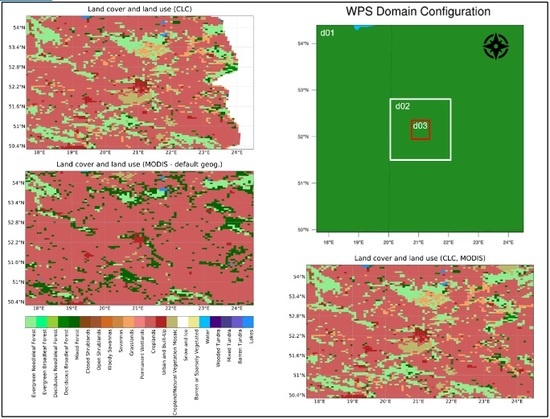
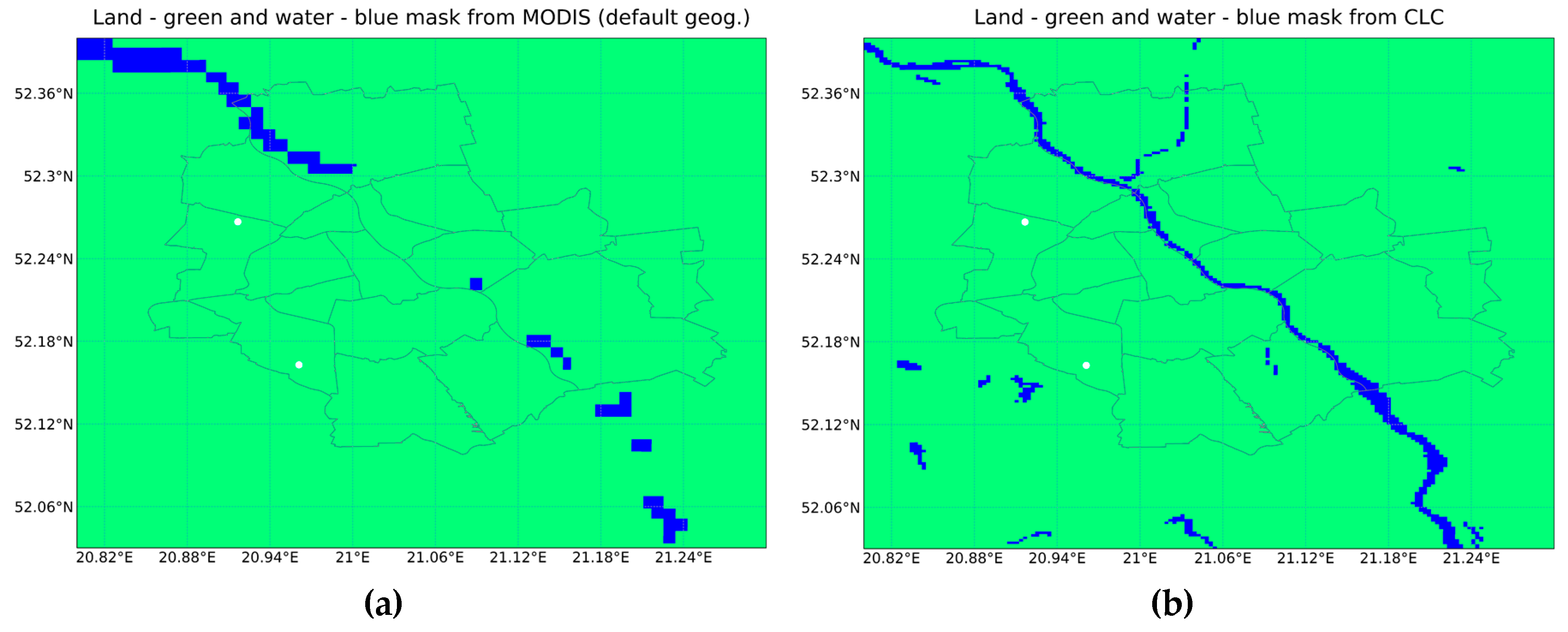
2.4. Land Use and Land Cover

In the conducted WRF model simulations the default geographical data about LULC were interpolated from MODIS IGBP 21-category data [11,42]. Moreover, the WRF can use 28-category (from WRF V3.8) LULC data provided by the USGS. These data were used as default in [4,6,7,25]. Therefore, as a part of research, a comparison between the USGS and MODIS IGBP category land dataset for the area of Warsaw was performed, as shown in Figure 2. For better reception on each visualization, with the spatial distribution of data and phenomena, the authors added borders of the city of Warsaw and its administrative districts. The location of the analyzed airports was presented in the figures with white dots. The EPBC airport is located in the northwestern and the EPWA is located in the southwestern part of Warsaw.
It has been noted that the MODIS data better represent current contours of Warsaw urban area [43], while the USGS data were inadequate and significantly outdated, compared to the CLC data. CLC 2018 data covers an urbanized area at least twice as large as USGS 30 arc seconds LULC. The expansion of urbanization in Warsaw noticeable in the MODIS and CLC data is also highlighted in scientific papers about the urbanization of the agglomeration’s agricultural areas [44,45,46,47].
To make the LULC information in the WRF model more up-to-date and detailed [48] we assimilated the CLC data, for the area of the experiment, to this NWP model. CLC 2018 data from the Copernicus servers with terrain resolution of 100 × 100 m were implemented to the WPS geographical data. To make this possible, it was necessary to reclassify 44 CLC classes into 21 MODIS IGBP classes, based on the authors’ scheme (Table 3) elaborated on the physical MODIS and the CLC classes concatenation confirmed by high-resolution satellite imagery information and data from topographic maps. The WRF model requires the same number of the geographical LULC classes for each domain, therefore the use of 28 USGS classes for the CLC reclassification would result in the necessity of using the USGS data for areas not covered by the CLC data. The nearest neighbor method was used to interpolate the CLC categorical data of LULC classes to the model grids. For the MODIS data interpolation the same method was used.
The reclassification process of the LULC data from the CLC to MODIS IGBP 21 classes, based on the scheme from Table 3, was conducted using the ArcGIS software. The CLC raster projection was changed from the original ETRS89 to the WGS84 which is compatible with the WRF model projection. The obtained result is shown in Figure 2c.
Although CLC consists of 11 classes for the anthropogenic areas, all of them were assigned to one urban class. It is possible to divide the urban area into more classes, as shown in Table 4, nevertheless, this operation is pointless in this study as the Urban Canopy Parameters (UCP) are not specified for the area of experiment yet. The urban classes High-Intensity Residential, Low-Intensity Residential, and Commercial, without defined UCP, have the same values of the physical parameters as Urban and Built-Up LULC class.
The usage of CLC as a LULC source in the WRF model improved the details in the representation of the Vistula river (Figure 3).
In NWP models water reservoirs cause variations in surface temperature and roughness which can influence changes in heat flux and local air circulation. Synoptic cases when the Vistula river modified the characteristics of the motion path of storm cells were observed.

2.5. Terrain Elevation Data

The terrain can significantly modify the direction of airflow and the amount of insolation in the lower atmosphere. Therefore, proper representation of landform is crucial for NWP models. The USGS Global Multi-resolution Terrain Elevation Data (GMTED2010) with horizontal resolution of 30 arc-seconds are default topography data in the WRF model. These elevation data are default for the WRF model as they are available for the entire globe [12,49]. For the area of interest, the authors implemented topography with higher, 3 arc seconds resolution from the National Geospatial-Intelligence Agency SRTM Digital Terrain Elevation Data. The SRTM data cover the land surface between 60°N and 56°S [49,50,51,52,53]. For the interpolation of continuous datasets of topography from the SRTM data and the GMTED2010 data to the simulation domain the following interpolation methods were used: the model grid-cell average (4.0), the four-point bilinear interpolation and the simple four-point average interpolation method [12]. If one interpolation method from the above mentioned in the given order could not be used, for example when the topography file had areas of missing values the four-point bilinear interpolation method could not be used, then the next method was used. The model grid-cell average (4.0) interpolating method can be used for interpolating higher resolution geographical data to lower resolution model grid. This method averages the values of pixels which are included at the model grid (all or most of it). The option 4.0 in this method means the minimum ratio of the source geographical data to the model grid resolution for which the data will be applied. In the conducted simulations, this method could be used only for the first (5 × 5 km) and the second (1 × 1 km) domains. For the third domain (200 × 200 m) the other two of these methods were used. The four-point bilinear interpolation method is simply a connection of two linear interpolations for searching the x and y coordinates of the model grid nodes from their nearest four coordinates. The simple four-point average interpolation method works as a four-point bilinear interpolation method, but it does not need four valid points to process interpolation. This method averages the value of the point from the available points and requires at least one valid source data point to process the interpolation. The methods used for the data interpolation in the WRF are described in the WRF Fortran source code [12].
As a result of the SRTM elevation dataset adaptation, the terrain representation in the computational domain has improved markedly. The comparison of these two topographies is summarized in Figure 4. On the outline from the SRTM data, more variable riverbed and more details in terrain denivelation are highlighted. Additionally, it is visible how the increase of the model resolution highlights the landform, for example in the picture obtained using the SRTM topography, the remnants of a closed landfill are clearly distinguishable on the west side of the EPBC airfield (yellow-colored blob).

2.6. WRF Binary Format—Methods of Generation
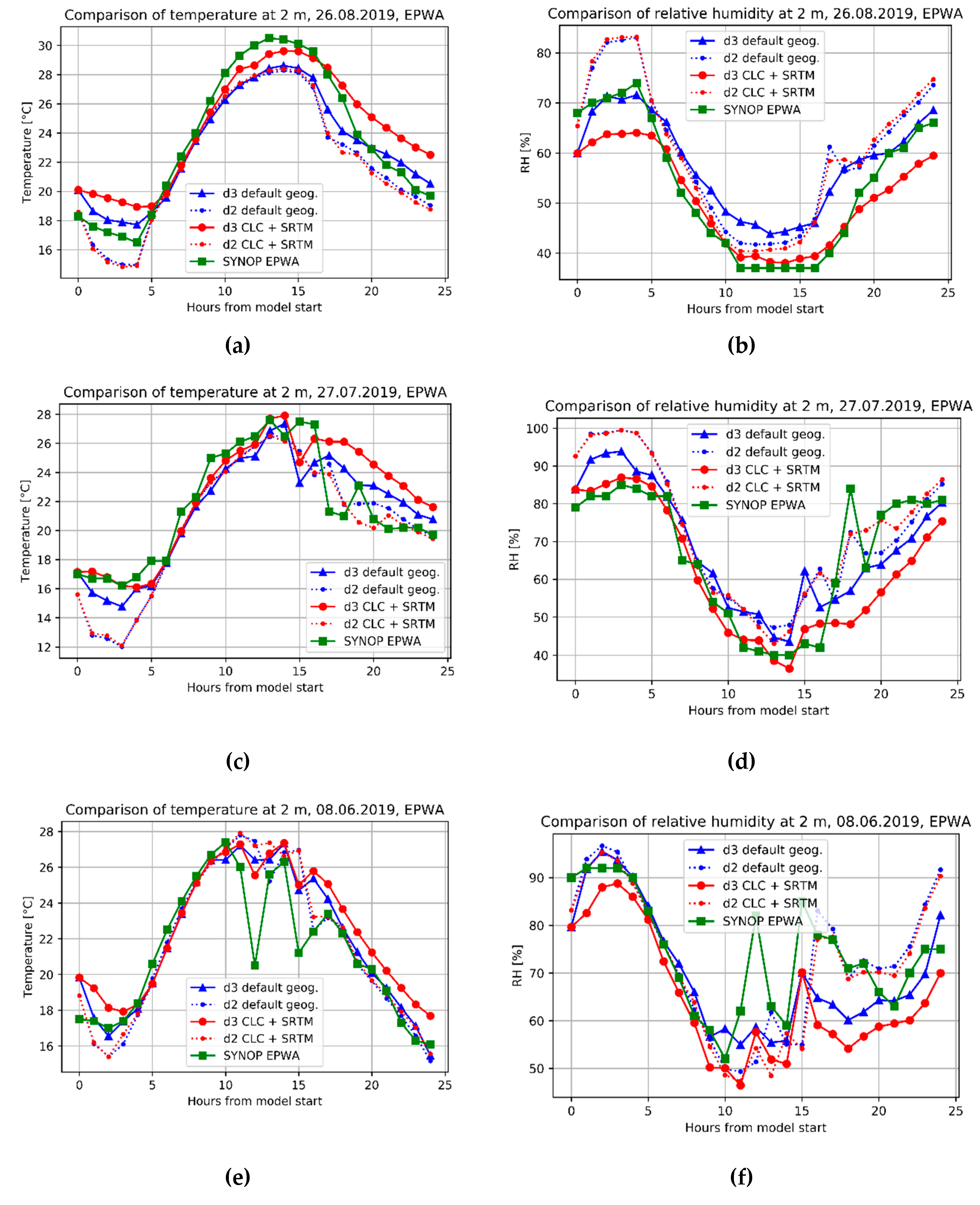
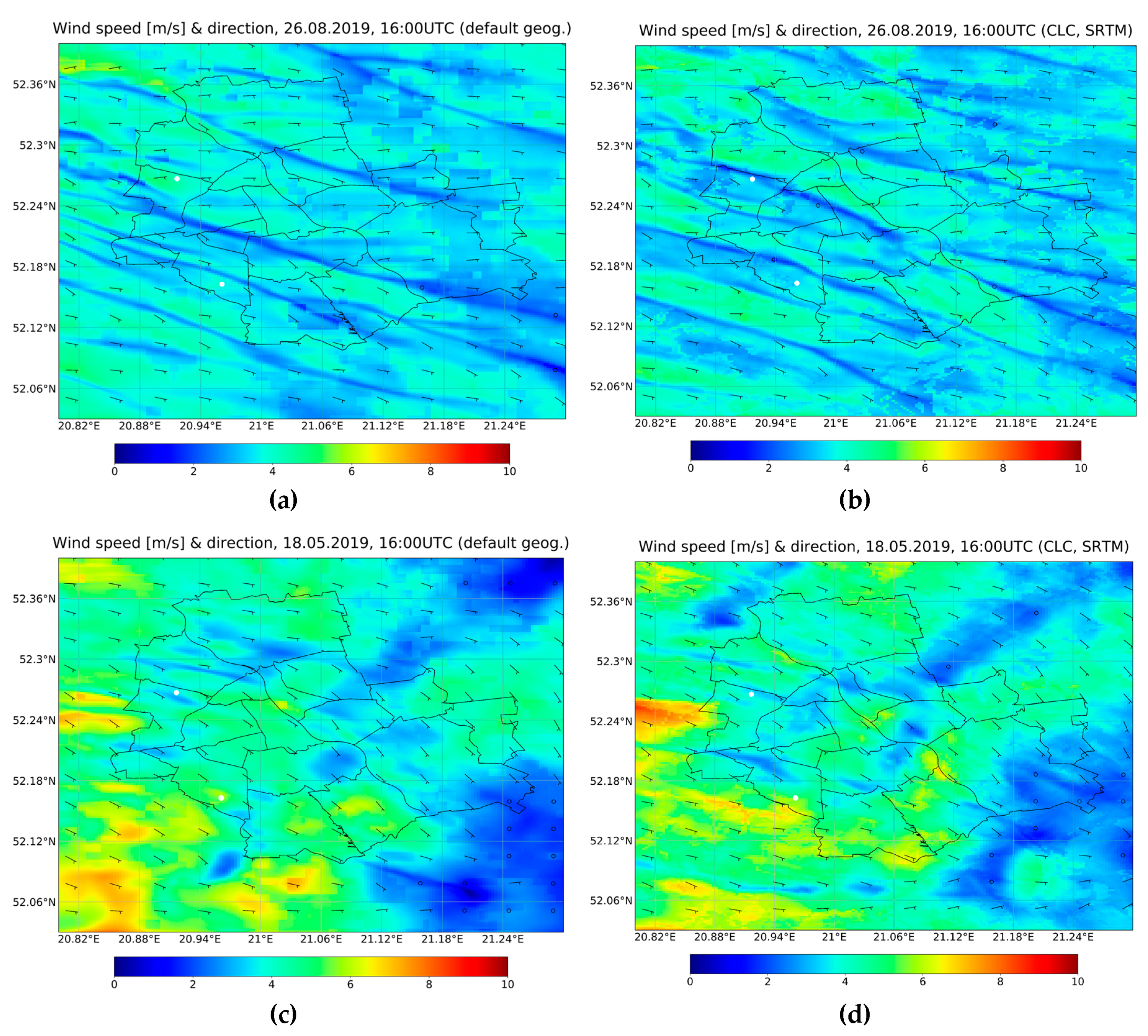
The WRF model geographic data are written in the binary format [12,14] which is read by the WPS. The new geographic data in GeoTIFF format from CLC and SRTM was processed to the format interpreted by the WRF model. During this study, three independent methods (tools) of producing the WRF binary format were examined: QGIS-GIS4WRF, ENVI, and CONVERT_GEOTIFF.
The binary products obtained by means of the above-mentioned programs are generated using various techniques, therefore it is advisable to visually check the results of the processing. Wrong results could also be obtained by incorrect creation of index files which are an integral part of the binary format batches. GIS4WRF is a new QGIS plugin [54] which provides users with a fast and automatic way of generating WPS binary format files. It is worth mentioning that the tiles of the binary files produced by GIS4WRF do not overlap. This plugin generates the index file automatically, like the CONVERT_GEOTIF open source program. However, a different reading pattern was noted for row order in the files for CONVERT_GEOTIFF than in other analyzed programs. Only ENVI, which is a driver for GDALL, requires self-creation of the index files. The final results of the conversion carried out by means of these three tools were identical.

3. Results

The obtained forecasts i.e., the values of the analyzed meteorological parameters from the WRF model simulations with default geographical data (MODIS, GMTED2010) and adapted geographical data of higher resolution (terrain (SRTM) and LULC (CLC 2018)) were evaluated by comparing them with observations. For this purpose, the Python programming language was used. This language allows reading data in the NetCDF format which is the output format of the WRF model [55]. The bilinear interpolation method was used to extract the exact values of meteorological parameters from the model results mesh. Separate charts were made to compare the WRF model output with default geographical data, and with results of the WRF model simulation with CLC and SRTM geographical data, and also with meteorological observations from the Warsaw airports (Figure 5 and Figure 6). Linear interpolation of the hourly measurements and the model forecasts was used to show the distribution of the analyzed meteorological parameters. The comparison of the results was presented for the second (1 × 1 km) and third (200 × 200 m) domains. The first domain was omitted in the results comparison because of its low resolution (5 × 5 km), no differences for the two different geographical datasets at this domain were obtained.
Based on the results presented in Figure 6, it was found that the temperature obtained with the CLC and SRTM geographical data is slightly higher during the day, which yields better forecasting of the maximum temperature value. Contrary, the forecast value of the maximum temperature by the default WRF model is generally underestimated. In some situations (Figure 6c,d) the improvement of the obtained values of the analyzed parameters was achieved during the spin-up time (the first 6 h of a model run) for which the forecast is commonly rejected because of the instability of the model during its first hours of run. Although default geographical data (MODIS, GMTED2010) were generally consistent with the higher resolution (CLC, SRTM) geographical data, in the case of results for the third domain there was a noticeable positive impact of the higher resolution geographical data adoption on the produced forecasts. For the second domain calculations, the impact was in most cases low or unnoticeable.
As a result of the default geographical data change to CLC and SRTM, the higher detail and different values of horizontal distribution of meteorological parameters were noticed. The changes also result in changes of the speed of movement of atmospheric fronts (Figure 7). The comparison with meteorological radar data [33] shows that in this case faster movement of the atmospheric front, visible in Figure 7b, better corresponds to observational data.
The distribution of the obtained meteorological fields in other point in Warsaw was also analyzed (Figure 5). In the case of the EPBC location, the geographical data modification did not change the obtained results significantly. This was probably because the implementation of CLC data did not cause significant changes in LULC for the area of the EPBC. The Babice airport is located in the vicinity of the Kampinoski National Park at the border of the Urban and Built-Up area. Implementation of CLC caused very small changes in LULC of the neighborhood of the EPBC airport. By increasing the resolution of geographical data of LULC, the EPWA airport was surrounded by more Urban and Built-Up area, also few ponds, Croplands and Grassland appeared on the west side of the airport. As demonstrated in Figure 5, the change of the grid computing from domain 2 (grid: 500 × 500 m) to domain 3 (grid: 200 × 200 m) allowed capture of the results improvement.
The wind speed and direction fields obtained from the WRF model using default and higher resolution geographical data are shown in Figure 8.
Comparing wind speed and direction distribution during the high-pressure system over Poland, Figure 8a,b, the air corridors appeared on areas that are free from Urban and Built-Up class. The air corridors were depicted more properly on the field calculated using higher resolution geographical data. Changes in wind speed and direction were also noticeable (Figure 9) for the geographical data from various sources used in the WRF simulations. The verification of wind fields is a significant challenge due to the fast-changing nature of this parameter and its dependence on the roughness of the ground, i.e., distribution of density and height of terrain obstacles causing a decrease in wind speed. Wind fields obtained using higher resolution geographical data (CLC and SRTM) are characterized by not only greater diversity of the wind field but also by changes in the obtained values of wind speed and direction. The obtained values of wind speed for the analyzed places were, in general, lower than those obtained with the default geographical data, and they better agreed with the observations from the EPBC airport. For the EPWA airport the values were underestimated.

Verifiability of Meteorological Parameters

The results verification included a comparison of the meteorological parameters forecast from the WRF simulations with the default geog. data (MODIS and GMTED2010) and the higher resolution geog. data (CLC and SRTM) with the observations. The verification statistics of the results based on seven random synoptic situations are summarized in Table 5 and Table 6, where their average values are presented separately for the individual analyzed locations (EPWA and EPBC).
Based on the results of the ME value it can be seen that using the CLC and the SRTM data in the model results in higher values of the forecast temperature which, especially in the case of EPBC, were very similar to the observations. Increasing the value of the forecasted temperature resulted in reducing the value of the predicted relative humidity, which was also closer to measurements at the EPBC station. The use of the CLC and the SRTM geography contributed to the reduction of wind speed compared to the results obtained by using default geog. data and the substantial upgrade of the forecast of the wind direction value for the EPWA airport. The value of MAE indicates an improvement in temperature and relative humidity at the EPWA after the CLC and the SRTM data adoption. The MSE and RMSE values indicate large error values of wind direction. Due to the high variability of this parameter in time and space (especially during atmospheric fronts passages), it is difficult to forecast the parameter. The R value indicates the positive influence of the CLC and SRTM data on the wind speed and relative humidity forecast for both locations, compared to results obtained from the model running on default geographical data.
Analyzing the RMSE error detailed distributions for each analyzed case, presented in Table 7 and Table 8, it was noticed that for EPWA in two out of the seven analyzed situations the RMSE value of the forecast temperature on higher resolution geog. data was greater than the one obtained for the temperature forecast on default geog. data. In the case of EPBC three out of the seven forecasts of temperature on higher resolution geog. data revealed greater RMSE than the forecast obtained on the default data. Analyzing the RMSE error for relative humidity in both cases (EPWA and EPBC) for three out of the seven analyzed situations the RMSE value of relative humidity forecast was higher for the model simulations obtained on high-resolution geog. data than the one obtained on simulations with the default geog. data.
The detailed distribution of the RMSE value for particular analyzed situations indicates the significant reduction of the wind speed on the EPWA airport in comparison to the observations after higher resolution geog. data implementation. The increase of urban area on CLC data around EPWA airport in comparison to MODIS data resulted in increased roughness at this airport localization. Lowering the value of RMSE of wind speed after higher resolution geog. data adoption indicates an improvement of their representation for EPWA localization. The observed better representation of the arrangement of the urban class areas around EPWA airport on higher resolution geog. data is the possible reason for this improvement. Generally, lower values of the RMSE were noticed for EPBC airport, which indicates a better representation of wind speed and direction at this location after higher resolution geog. data adoption.

4. Discussion

In this paper, we evaluated the impact of the high resolution CLC and the SRTM topography on the estimation accuracy of the weather model parameters at the WRF microscale simulations (200 × 200 m) for Warsaw. In presented studies, the novel method of implementation of the CLC data to the WRF simulations in which the first calculational domains cover areas out of the CLC data coverage was proposed. The obtained statistical values for grid lower than 1 km indicate that this method successfully enabled the authors to implement the CLC data to the WRF model simulations for such problematic areas. The obtained results of the increased maximum temperature value after adoption of the CLC data to the simulations are consistent with those obtained by [4,6,7,25]. Unlike the existing studies of the CLC data adoption to the WRF model, the results of the simulations with use of the CLC data conducted by the authors were compared to the outputs of simulations with the MODIS default data, which are more up to date then the USGS data, and could automatically influence the improvement of the obtained results for the WRF default simulations. In previous, even very recent studies, the default simulations made to compare the CLC data adoption to the WRF were conducted with the USGS data used as default [4,6,7,25].
The obtained results of the conducted WRF simulations indicate that the influence of changing the default geographical data (MODIS and GMTED2010) to higher resolution geographical data (CLC and SRTM), in most cases yielded more accurate values of temperature and relative humidity at 2 m. The analysis demonstrates that in the case of EPWA the results of simulation using higher resolution geographical data showed no improvement of the wind speed values. The values were mostly underestimated. For this location only slight improvement of wind direction was noticed after the adoption of higher resolution geog. data. However, the model results of wind speed and direction changes on CLC and SRTM geographical data better represent changes of these parameters occurring in the natural environment of the EPBC meteorological station—in most cases, the obtained wind parameters values were closer to the observations. A possible reason of decreasing wind speed distribution by the WRF model after CLC and SRTM geographical data adoption could be due to too high surface roughness in the model [4,10,11,30] in the place of the EPWA airfield where the synoptic observations were made. The EPWA airport is a larger area than the aeroclub airport EPBC located in the city border zone, in the vicinity of forests. Adjustment of classes from CLC to possible MODIS meant that EPWA airport is situated in the Urban and Built-Up area, what reduced the wind strength received for EPWA from the model. The EPWA airport is surrounded by compact buildings but the airport area itself is a large open area. It is worth noting that the synoptic situations observed in the analyzed period had an important influence on the obtained verification statistics. The authors obtained much better verification statistic results for high-pressure systems than for frontal synoptic situations, during which temporary changes in the meteorological parameters are significant.
Furthermore, the obtained results of the estimation accuracy of the weather model parameters indicate some limitations of the CLC data and the SRTM topography adoption on the microscale WRF simulations for Warsaw which were especially visible in the wind field parameters simulations accuracy. The level of limitation was different for specific examined locations, and depended on how the basic description of the physical parameters of the Urban and Built-Up class was consistent with the real conditions at the given location. In order to overcome these limitations, our future research will focus on improving the high-resolution geographical data adoption (CLC, SRTM) by taking into account high-resolution urban data sets (e.g., height, shape, and density of buildings, and spatial structure of streets—direction and width) for describing the particular grid of the CLC Urban and Built-Up class. To activate module called the Urban Canopy Model (UCM) in the WRF model it is necessary to develop proper fields to describe the morphology of the city for better representation of its aerodynamic properties. LIDAR scans of the object heights, the Topographic Object Database (BDOT10k) corresponding to the detail of the map at the scale of 1:10,000, and 3D CityGML Database could be valuable information sources for creating the fields for the Warsaw agglomeration. The fields which enable to describe the urban morphology in detail will be developed by the authors for the Warsaw agglomeration and their implementation results will be presented in future research reports. This approach is essential for further improvement of the accuracy of the meteorological parameters microscale simulations, especially for wind field parameters whose results will be verified based on the meteorological observations and the precinct ventilation zones [56] in the city, which take into account urban form compactness, height of buildings, and structure of streets. The results of the WRF with the UCM module may also provide initial and boundary conditions for fine scale urban transport and diffusion models for studying local ventilation performance and urban planning.

5. Conclusions

In this study we evaluated the impact of the high resolution CLC and the SRTM topography on the estimation accuracy of the weather model parameters in the WRF microscale simulations (200 × 200 m) for Warsaw. Moreover, new, higher resolution geographical data to the WRF model for Warsaw were implemented by means of the method of adoption of the CLC data for the border areas proposed by the authors. For this purpose, the authors’ reclassification algorithm for the CLC data to MODIS classes was implemented. Based on the conducted experiments and their verification, the correctness of the proposed method was proven. In places where the changes of LULC were greater, the changes of the estimated parameters were also more significant. It was necessary to increase the model resolution to observe the changes. The results of the comparison of the weather forecasts produced with high resolution geographical data (CLC, SRTM) and default geographical data (MODIS, GMTED2010) with the surface observations demonstrate that it is possible to increase the accuracy of the forecast results by using higher resolution geographical data (CLC, SRTM) and by simultaneously increasing the model domain resolution in the WRF mode. It was also demonstrated that the obtained values of the RMSE were generally higher for the microscale simulations with default geographical data (MODIS, GMTED2010), especially for temperature and relative humidity at 2 m, than those obtained from the calculation on high-resolution geographical data (CLC, SRTM). The results obtained for the wind field did not give the same improvement for both analyzed places. Further implementation of the data about the urban morphology to the particular grid of the Urban and Built-Up class in the WRF model could potentially contribute to obtaining more accurate results, especially for wind speed simulations in which the obtained results were not satisfying.
Based on the conducted studies, the authors proved that for the microscale simulations it is advisable to use CLC data rather than MODIS data, even for places that first calculation domains include areas out of the CLC coverage. As a result of this study the authors also improved the WRF model for Warsaw by increasing the resolution of the model calculation domain and by implementing higher resolution basic geographical data about LULC and terrain height to the WRF model. More research will be conducted to further improve the accuracy of the computed meteorological parameters by adopting more detailed descriptions of the city by the urban morphology fields implementation to the WRF model.

Author Contributions

All authors contributed to conducting this research. Conceptualization, methodology, software, K.K. and J.S., validation, formal analysis, investigation, resources, data curation J.S.; supervision K.K.; writing—original draft preparation, J.S.; writing—review and editing, K.K.; visualization, J.S. All authors have read and agreed to the published version of the manuscript.

Funding

This research was funded by the Military University of Technology, Faculty of Civil Engineering and Geodesy, Institute of Geospatial Engineering, Department of Military Hydrometeorology and Geomatics.

Acknowledgments

The Institute of Meteorology and Water Management—National Research Institute as well as the NOAA National Weather Service, National Centers for Environmental Prediction that were the sources of the meteorological data used to prepare this paper.

Conflicts of Interest

The authors declare no conflict of interest. All regulations and restrictions of data use can be found at: https://www.weather.gov/privacy, https://www.doi.gov/privacy, https://dane.imgw.pl/regulations, http://danepubliczne.imgw.pl and https://land.copernicus.eu/terms-of-use.

References

  1. Petrişor, A.I. Using CORINE data to look at deforestation in Romania: Distribution & possible consequences. Urbanism. Arhit. Construcţii 2015, 6, 83–90. [Google Scholar]
  2. Thibbotuwawa, A.; Bocewicz, G.; Nielsen, P.; Banaszak, Z. Planning deliveries with UAV routing under weather forecast and energy consumption constraints. IFAC-PapersOnLine 2019, 52, 820–825. [Google Scholar] [CrossRef]
  3. Oleniacz, R.; Rzeszutek, M. Intercomparison of the CALMET/CALPUFF Modeling System for Selected Horizontal Grid Resolutions at a Local Scale: A Case Study of the MSWI Plant in Krakow, Poland. Appl. Sci. 2018, 8, 2301. [Google Scholar] [CrossRef] [Green Version]
  4. De Meij, A.; Vinuesa, J.F. Impact of SRTM and Corine Land Cover data on meteorological parameters using WRF. Atmos. Res. 2014, 143, 351–370. [Google Scholar] [CrossRef]
  5. Huang, M.; Wang, Y.; Lou, W.; Cao, S. Multi-scale simulation of time-varying wind fields for Hangzhou Jiubao Bridge during Typhoon Chan-hom. J. Wind Eng. Ind. Aerodyn. 2018, 179, 419–437. [Google Scholar] [CrossRef]
  6. Li, H.; Wolter, M.; Wang, X.; Sodoudi, S. Impact of land cover data on the simulation of urban heat island for Berlin using WRF coupled with bulk approach of Noah-LSM. Theor. Appl. Climatol. 2018, 134, 67–81. [Google Scholar] [CrossRef]
  7. De Meij, A.; Zittis, G.; Christoudias, T. On the uncertainties introduced by land cover data in high-resolution regional simulations. Meteorol. Atmos. Phys. 2019, 131, 1213–1223. [Google Scholar] [CrossRef]
  8. Gondocs, J.; Breuer, H.; Pongracz, R.; Bartholy, J. Urban heat island mesoscale modelling study for the Budapest agglomeration area using the WRF model. Urban Clim. 2017, 21, 66–86. [Google Scholar] [CrossRef]
  9. Karsisto, V.; Nurmi, P.; Kangas, M.; Hippi, M.; Fortelius, C.; Niemela, S.; Järvinen, H. Improving road weather model forecast by adjusting the radiation input. Meteorol. Appl. 2016, 23, 503–513. [Google Scholar] [CrossRef] [Green Version]
  10. Calvo-Sánchez, J.; Morales-Martin, G. Wind Field Deterministic Forecasting. In Wind Field and Solar Radiation Characterization and Forecasting. A Numerical Approach for Complex Terrain; Perez, R., Ed.; Springer: Basel, Switzerland, 2018; pp. 113–128. [Google Scholar] [CrossRef]
  11. Carvalho, D.; Rocha, A.; Silva Santos, C.; Pereira, R. Wind resources modelling in complex terrain different mesoscale-microscale coupling techniuques. Appl. Energy 2013, 108, 493–504. [Google Scholar] [CrossRef] [Green Version]
  12. Wang, W.; Bruyère, C.; Duda, M.; Duda, M.; Dudhia, J.; Gill, D.; Kavulich, M.; Werner, K.; Chen, M.; Lin, H.-C.; et al. Weather Research & Forecasting Model. ARW Version 4 Modeling System User’s Guide; Mesoscale and Microscale Meteorology Laboratory NCAR: Boulder, CO, USA, 2019; Available online: https://www2.mmm.ucar.edu/wrf/users/docs/user_guide_V4/WRFUsersGuide.pdf (accessed on 20 April 2020).
  13. Chen, F.; Liu, Y.; Kusaka, H.; Tewari, M.; Bao, J.W.; Lo, C.F.; Lau, K.H. Challenge of Forecasting Urban Weather with NWP Models. In Proceedings of the First Joint WRF/MM5 User’s Workshop, Boulder, CO, USA, 22–25 June 2004. [Google Scholar]
  14. Beezley, J.D.; Kochanski, A.K.; Kondratenko, V.Y.; Mandel, J. Integrating high-resolution static data into WRF for real fire simulations. In Proceedings of the Ninth Symp. Fire For. Meteorol., Palm Springs, CA, USA, 18–20 October 2011. [Google Scholar]
  15. Chen, F.; Kusaka, H.; Bornstein, R.; Ching, J.; Grimmond, C.S.B.; Grossman-Clarke, S.; Loridan, T.; Manning, K.W.; Martilli, A.; Miao, S.; et al. The integrated WRF/urban modeling system: Development, evaluation, and applications to urban environmental problems. Int. J. Climatol. 2011, 31, 273–288. [Google Scholar] [CrossRef]
  16. Jose, R.S.; Pérez, J.L. Mesoscale meteorological models in the urban context. In Understanding Urban Metabolism, A Tool for Urban Planning; Chrysoulakis, N., de Castro, A., Moors, E.J., Eds.; Routeladge Press Taylor & Francis Group: London, UK; New York, NY, USA, 2015; pp. 69–78. ISBN 978-1-315-76584-6. [Google Scholar]
  17. Dimitrova, R. Modeling the Impact of Urbanization on Local Meteorological Conditions in Sofia. Atmosphere 2019, 10, 366. [Google Scholar] [CrossRef] [Green Version]
  18. Li, X.; Mitra, C.; Dong, L.; Yang, Q. Understanding land use change impacts on microclimate using Weather Research and Forecasting (WRF) Model. Phys. Chem. Earth 2018, 103, 115–126. [Google Scholar] [CrossRef]
  19. Trihamdani, A.R.; Kubota, T.; Lee, H.S.; Sumida, K.; Phuong, T.T.T. Impacts of Land Use Changes on Urban Heat Islands in Hanoi, Vietnam: Scenario Analysis. Procedia Eng. 2017, 198, 525–529. [Google Scholar] [CrossRef]
  20. Schicker, I.; Arnold Arias, D.; Seibert, P. Influences of updated land-use datasets on WRF simulations for two Austrian regions. Meteorol. Atmos. Phys. 2016, 128, 279–301. [Google Scholar] [CrossRef]
  21. Chen, L.; Ma, Z.; Fan, X. A comprehensive study of two land surface schemes in WRF model over Eastern China. J. Trop. Meteorol. 2012, 18, 445–456. [Google Scholar]
  22. Jandaghian, Z.; Akbari, H. The Effect of Increasing Surface Albedo on Urban Climate and Air Quality: A Detailed Study for Sacramento, Houston, and Chicago. Climate 2018, 6, 19. [Google Scholar] [CrossRef] [Green Version]
  23. Morini, E.; Touchaei, A.G.; Castellani, B.; Rossi, F.; Cotana, F. The Impact of Albedo Increase to Mitigate the Urban Heat Island in Terni (Italy) Using the WRF Model. Sustainability 2016, 8, 999. [Google Scholar] [CrossRef] [Green Version]
  24. Jancewicz, K. Remote Sensing Data in Wind Velocity Field Modelling: A Case Study from the Sudetes (SW Poland). Pure Appl. Geophys. 2014, 171, 941–964. [Google Scholar] [CrossRef] [Green Version]
  25. Jiménez-Esteve, E.B.; Udina, M.; Soler, M.R.; Pepin, N.; Miró, J.R. Land use and topography influence in complex terrain area: A high resolution mesoscale modeling study over the Eastern Pyrenees using the WRF model. Atmos. Res. 2017. [Google Scholar] [CrossRef] [Green Version]
  26. Jancewicz, K.; Szymanowski, M. The Relevance of Surface Roughness Data Qualities in Diagnostic Modelling of Wind Velocity in Complex Terrain: A Case Study from the Śnieżnik Massif (SW Poland). Pure Appl. Geophys. 2017, 174, 569–594. [Google Scholar] [CrossRef] [Green Version]
  27. Feranec, J.; Soukup, T.; Hazeu, G.; Jaffrain, G. (Eds.) European Landscape Dynamics: CORINE Land Cover Data, 1st ed.; CRC Press: Boca Raton, FL, USA, 2016; ISBN 9781315372860. [Google Scholar]
  28. Büttner, G. CORINE Land Cover and Land Cover Change Products. In Land Use and Land Cover Mapping in Europe: Practices & Trends; Manakos, I., Braun, M., Eds.; Springer: Dordrecht, The Netherlands, 2014; pp. 55–74. ISBN 978-94-007-7969-3. [Google Scholar]
  29. Büttner, G.; Kosztra, B. CLC 2018, Technical Guidelines; Service Contract No 3436/R0-Copernicus/EEA.56665; EEA: Wien, Austria, 2017; ISBN 92-9167-511-3. [Google Scholar]
  30. Luc, M.; Bielecka, E. Ontology for National Land Use/Land Cover Map: Poland Case Study. In Land Use and Land Cover Semantics; Ahlqvist, O., Varanka, D., Fritz, S., Janowicz, K., Eds.; CRS Press Taylor & Francis Group: Boca Raton, FL, USA, 2015; pp. 21–40. [Google Scholar]
  31. Pineda, N.; Jorba, O. Using NOAA AVHRR and SPOT VGT data to estimate surface parameters: Application to a mesoscale meteorological model. Int. J. Remate Sens. 2004, 25, 129–143. [Google Scholar] [CrossRef]
  32. Anderson, J.R.; Hardy, E.E.; Roach, J.T.; Witmer, R.E. A Land Use and Land Cover Classification System for Use with Remote Sensor Data, 4th ed.; United States Government Printing Office: Washington, DC, USA, 1983.
  33. Kumar, A.; Chen, F.; Barlage, M.; Ek, M.B.; Niyogi, D. Assessing Impact of Integrating MODIS Vegetation Data in the Weather Research and Forecasting (WRF) Model Coupled to Two Different Canopy-Resistance Approaches. J. Appl. Meteorol. Climatol. 2014, 53, 1362–1380. [Google Scholar] [CrossRef]
  34. Institute of Meteorology and Water Management—National Research Institute, Archive of Meteorological Observations. Available online: https://www.danepubliczne.imgw.pl (accessed on 29 April 2020).
  35. Czernecki, B.; Głogowski, A.; Nowosad, J. Climate: An R Package to Access Free In-Situ Meteorological and Hydrographical Datasets for Environmental Assessment. Sustainability 2020, 12, 394. [Google Scholar] [CrossRef] [Green Version]
  36. Jolliffe, I.T.; Stephenson, D.B. Forecast. Verification: A Practitioner’s Guide in Atmospheric Science, 2nd ed.; John Wiley & Sons: Chichester, UK, 2012; ISBN 978-0-470-66071-3. [Google Scholar]
  37. Kendzierski, S.; Czernecki, B.; Kolendowicz, L.; Jaczewski, A. Air temperature forecasts’ accuracy of selected short-term and long-term numerical weather prediction models over Poland. Geofizyka 2018, 35, 19–37. [Google Scholar] [CrossRef]
  38. Solon, J.; Borzyszkowski, J.; Bidłasik, M.; Richling, A.; Badora, K.; Balon, J.; Brzezińska-Wójcik, T.; Chabudziński, Ł.; Dobrowolski, R.; Grzegorczyk, I.; et al. Physico-geographical mesoregions of Poland: Verification and adjustment of boundaries on the basis of contemporary spatial data. Geogr. Pol. 2018, 91, 143–170. [Google Scholar] [CrossRef]
  39. Zegara, T. Statistical review of Warsaw 4th Quarter 2019, 2020, XXVIII, pp. 37–43. Available online: https://warszawa.stat.gov.pl/ (accessed on 20 April 2020).
  40. Skamarock, W.C.; Klemp, J.B.; Dudhia, J.; Gill, D.O.; Liu, Z.; Berner, J.; Wang, W.; Powers, J.G.; Duda, M.G.; Barker, D.M.; et al. A Description of the Advanced Research WRF Model. Version 4; (No. NCAR/TN-556+STR); National Center for Atmospheric Research: Boulder, CO, USA, 2019. [Google Scholar] [CrossRef]
  41. The Global Forecasting System (GFS) of the National Weather Service NCEP. Available online: https://www.nco.ncep.noaa.gov/pmb/products/gfs/ (accessed on 29 April 2020).
  42. Friedl, M.A.; McIver, D.K.; Hodges, J.C.F.; Zhang, X.Y.; Muchoney, D.; Strahler, A.H.; Woodcock, C.E.; Gopal, S.; Schneider, A.; Cooper, A.; et al. Global land cover mapping from MODIS: Algorithms and early results. Remote Sens. Environ. 2002, 83, 287–302. [Google Scholar] [CrossRef]
  43. Golenia, M.; Zagajewski, B.; Ochtyra, A. Semiautomatic land cover mapping according to the 2nd level of the CORINE Land Cover legend. Pol. Cartogr. Rev. 2015, 47, 203–212. [Google Scholar] [CrossRef] [Green Version]
  44. Pabjanek, P.; Szumacher, I. Land use and ecosystem services temporal changes in the urban sprawl zone, Warsaw, Poland. Probl. Landsc. Ecol. 2017, XLIV, 29–40. [Google Scholar]
  45. Cieślak, I.; Białozior, A.; Szuniewicz, K. The Use of the CORINE Land Cover (CLC) Database for Analyzing Urban Sprawl. Remote Sens. 2020, 12, 282. [Google Scholar] [CrossRef] [Green Version]
  46. Solon, J. Spatial context of urbanization: Landscape pattern and changes between 1950 and 1990 in the Warsaw metropolitan area, Poland. Landsc. Urban. Plan. 2009, 93, 250–261. [Google Scholar] [CrossRef] [Green Version]
  47. Turner, B.; Meyer, W.B.; Skole, D.L. Global land use/land cover change: Towards an integrated study. AMBIO 1994, 23, 91–95. [Google Scholar]
  48. Copernicus Land Monitoring Service. Available online: https://land.copernicus.eu/ (accessed on 29 April 2020).
  49. Danielson, J.J.; Gesch, D.B. Global Multi-Resolution Terrain Elevation Data 2010 (GMTED2010), Open-File Report 2011–1073; U.S. Department of the Interior: Mission, SD, USA; U.S. Geological Survey: Reston, VA, USA; Rolla Publishing Service Center: Rolla, MO, USA, 2011. Available online: https://pubs.usgs.gov/of/2011/1073/pdf/of2011-1073.pdf (accessed on 20 April 2020).
  50. Van Zyl, J.J. The Shuttle Radar Topography Mission (SRTM): A breakthrough in remote sensing of topography. Acta Astronaut. 2001, 48, 559–565. [Google Scholar] [CrossRef]
  51. U.S. Geological Survey (USGS). Shuttle Radar Topography Mission (SRTM) Void Filled. Available online: https://earthexplorer.usgs.gov/ (accessed on 29 April 2020).
  52. Farr, T.G.; Rosen, P.A.; Caro, E.; Crippen, R.; Duren, R.; Hensley, S.; Kobrick, M.; Paller, M.; Rodriguez, E.; Roth, L.; et al. The Shuttle Radar Topography Mission. Rev. Geophys. 2007, 45. [Google Scholar] [CrossRef] [Green Version]
  53. Rodriguez, E.; Morris, C.S.; Belz, J.E. A global assessment of the SRTM performance. Photogramm. Eng. Remote Sens. 2006, 72, 249–260. [Google Scholar] [CrossRef] [Green Version]
  54. Meyer, D.; Riechert, M. Open source QGIS toolkit for Advanced Research WRF modeling system, Environment Modelling and Software. Environ. Model. Softw. 2019, 166–178. [Google Scholar] [CrossRef] [Green Version]
  55. Ladwig, W. Wrf-Python; Version 1.3.2; UCAR/NCAR: Boulder, CO, USA, 2017. [Google Scholar] [CrossRef]
  56. He, B.-J.; Ding, L.; Prasad, D. Enhancing urban ventilation performance through the development of precinct ventilation zones: A case study based on the Greater Sydney, Australia. Sustain. Cities Soc. 2019, 47, 101472. [Google Scholar] [CrossRef]
Figure 1. Visualization of the authors’ method for attaching the CORINE Land Cover (CLC) data to the WRF model for the CLC border areas, where first mesoscale calculation domains go beyond areas of the CLC coverage.
Remotesensing 12 01881 g001
Figure 2. Comparison between land use and land cover data in the WRF model simulations for Warsaw, domain 3 (200 × 200 m) and: (a) MODIS (used as default geog.) data; (b) USGS data; (c) CLC data.
Remotesensing 12 01881 g002
Figure 3. The water mask used in the WRF model for Warsaw from (a) MODIS data (default); (b) CLC data.
Remotesensing 12 01881 g003
Figure 4. Terrain height used in the WRF simulations for domain 3 (200 × 200 m) with (a) GMTED2010 topography; (b) SRTM topography.
Remotesensing 12 01881 g004
Figure 5. Example of the obtained values of temperature at 2 m (AGL) for 26.08.2019 at the airport (a) EPWA; (b) EPBC.
Remotesensing 12 01881 g005
Figure 6. Examples of the obtained values of air temperature and relative humidity at 2 m (AGL) in various synoptic situations: (a,b) high-pressure systems; (cf) atmospheric fronts.
Remotesensing 12 01881 g006
Figure 7. Example of the obtained values of meteorological parameters during frontal synoptic situation on 08.06.2019 at 15:00 UTC. Horizontal distribution of temperature at 2 m (°C) obtained with (a) default geographical data; (b) CLC and SRTM geographical data. Horizontal distribution of relative humidity (%) obtained with (c) default geographical data; (d) CLC and SRTM geographical data.
Remotesensing 12 01881 g007
Figure 8. Example of wind speed (m/s) and direction distribution (wind barbs) on 26.08.2019, 16:00 UTC obtained with (a) default geographical data; (b) CLC and SRTM geographical data. Example of wind speed (m/s) and direction distribution (wind barbs) on 18.05.2019, 16:00 UTC obtained with (c) default geographical data; (d) CLC and SRTM geographical data.
Remotesensing 12 01881 g008
Figure 9. (a) Example of the obtained values of wind direction at domain 3 for the EPWA, 09.06.2019; (b) example of the obtained values of wind speed at domain 3 for the EPWA, 27.07.2019.
Remotesensing 12 01881 g009
Table 1. Location of meteorological station at the Warsaw airports.
Location of the AirportsCoordinates of the Airport Meteorological Stations
Remotesensing 12 01881 i001EPWA
52° 9′ 46″N (52.1629°N)
20° 57′ 40″E (20.9611°E)
110 m (AMSL)
Remotesensing 12 01881 i002EPBC
52° 16′ 0″N (52.2667°N)
20° 55′ 0″E (20.9167°E)
107 m (AMSL)
Table 2. The WRF model configuration used in the experiment.
ParametersDomains 1/2/3
WRF Version4.1
Spin up time, forecast time6 h, 24 h
Global model gridded data sourceGFS 0.25° × 0.25° (3 h interval) [41]
Spatial resolution5 × 5 km/1 × 1 km/200 × 200 m
Geographical data (prepared by the authors for high resolution simulations)CLC + MODIS + GMTED2010/CLC + SRTM/CLC + SRTM
Geographical data (default simulations)MODIS + GMTED2010/MODIS + GMTED2010/MODIS + GMTED2010
Vertical levels60/60/60
CumulusGrell-Freitas (Grell et al. 2013)—for all domains
MicrophysicsWSM6 (Hong and Lim, 2006)/-/-
Longwave radiationRRTMG (Jacono et al., 2008)—for all domains
Shortwave radiationRRTMG (Jacono et al., 2008)—for all domains
Surface layerRevised MM5 Monin-Obukhov scheme (Imenez et al., 2012)—for all domains
Planetary boundary layerYonsei University scheme—YSU (Hong et al. 2006)/YSU/-
Table 3. Scheme of the reclassification for the LULC categories from the CLC to modified IGBP MODIS classes.
Number of CLC ClassDescription of CLC ClassNumber of MODIS LULC ClassName of MODIS LULC Class
111–140, 142Urban/Artificial Surfaces13Urban and Built-Up
141Green Urban Areas4Deciduous Broadleaf Forest
211Non-irrigated Arable Land12Croplands
212Permanently Irrigated Land12Croplands
213Rice Fields12Croplands
221Vineyards14Cropland/Nat. Vegetat. Mosaic
222Fruit Trees or Berry Plantations14Cropland/Nat. Vegetat. Mosaic
223Olive Groves 14Cropland/Nat. Vegetat. Mosaic
231Pastures10Grassland
241Annual and Permanent Crops14Cropland/Nat. Vegetat. Mosaic
242Complex Cultivation Patterns14Cropland/Nat. Vegetat. Mosaic
243Mixed Agriculture and Natural Vegetation14Cropland/Natural Vegetation Mosaic
244Agro-Forestry Areas14Cropland/Nat. Vegetat. Mosaic
311Broad-Leaved Forest4Deciduous Broadleaf Forest
312Coniferous Forest1Evergreen Needleleaf Forest
313Mixed Forest5Mixed Forests
321Natural Grasslands10Grasslands
322Moors and Heathland7Open Shrublands
323Sclerophyllous Vegetation7Open Shrublands
324Transitional Woodland/Shrub7Open Shrublands
331Beaches, Dunes, Sands16Barren or Sparsely Vegetated
332Bare Rocks16Barren or Sparsely Vegetated
333Sparsely Vegetated Areas16Barren or Sparsely Vegetated
334Burnt Areas16Barren or Sparsely Vegetated
335Glaciers Perpetual Snow15Snow or Ice
411–423Inland Mashes, Peat Bogs, Salt Marshes, Salines, Intertidal Flats11Permanent Wetlands
511–522Inland Waters, Lagoons, Estuaries21Lakes
523Sea and Ocean17Water
Table 4. Scheme of reclassification for the urban area LULC categories, from CLC to MODIS classes.
Number
of CLC Class
Names of CLC Urban ClassesNumber of MODIS ClassName of MODIS LULC Class
111Continuous Urban Fabric32High-Intensity Residential
112Discontinuous Urban Fabric31Low-Intensity Residential
121Industrial or Commercial Units33Industrial or Commercial
122Road and Rail Networks or Associated Land33Industrial or Commercial
123Port Areas33Industrial or Commercial
124Airports33Industrial or Commercial
131Mineral Extraction Sites33Industrial or Commercial
132Dump Sites33Industrial or Commercial
133Construction Sites33Industrial or Commercial
141Green Urban Areas4Delicious Broadleaf Forest
142Sport and Leisure Facilities33Industrial or Commercial
Table 5. Average statistical evaluation of the simulations for EPWA: ME, MAE, RMSE, MSE, BIAS, and R statistics.
Parameters at EPWA
(Time 10:00–15:00 UTC)
MEMAERMSEMSEBIASR
Temperature (°C)default geog.−0.201.561.873.940.940.70
CLC + SRTM0.321.411.683.540.980.67
Relative humidity (%)default geog.1.438.119.3692.601.040.73
CLC + SRTM−3.857.548.4496.010.940.77
Wind speed (m/s2)default geog.−0.691.261.512.400.88−0.08
CLC + SRTM−1.061.481.783.280.79−0.02
Wind direction (°)default geog.10.5827.1331.581485.271.110.11
CLC + SRTM4.2629.3134.542021.311.080.28
Table 6. Average statistical evaluation of the simulations for EPBC: ME, MAE, RMSE, MSE, BIAS, and R statistics.
Parameters at EPBC
(Time 10:00–15:00 UTC)
MEMAERMSEMSEBIASR
Temperature (°C)default geog.−0.091.131.442.590.970.54
CLC + SRTM0.031.211.472.590.970.53
Relative humidity (%)default geog.0.206.197.2966.631.010.51
CLC + SRTM0.106.197.2565.521.000.53
Wind speed (m/s2)default geog.−0.241.191.582.961.01−0.41
CLC + SRTM−0.451.271.542.670.93−0.21
Wind direction (°)default geog.1.5032.3339.612712.301.050.03
CLC + SRTM11.4132.1837.312280.441.120.28
Table 7. RMSE for temperature (T), relative humidity (RH), wind speed (WS), and wind direction (WD) for the analyzed synoptic situations at EPWA, the period from 10:00 UTC to 15:00 UTC.
EPWARMSE
DATET
Default Geog.
T
CLC + SRTM
RH
Default Geog.
RH
CLC + SRTM
WS
Default Geog.
WS
CLC + SRTM
WD
Default Geog.
WD
CLC + SRTM
26.08.20191.931.007.821.651.122.1027.8724.87
27.07.20191.981.349.893.382.192.3643.3136.85
08.06.20192.932.7212.4214.441.671.8976.9194.49
20.05.20192.512.9711.3013.571.721.6520.6316.19
18.05.20191.732.068.6013.361.211.6835.3553.33
20.01.20201.221.0510.328.051.471.376.155.79
21.01.20200.780.645.194.661.171.3910.8110.26
MEAN1.871.689.368.441.511.7831.5834.54
Table 8. RMSE for temperature (T), relative humidity (RH), wind speed (WS), and wind direction (WD) for the analyzed synoptic situations at EPBC, the period from 10:00 UTC to 15:00 UTC.
EPBCRMSE
DATET
Default Geog.
T
CLC + SRTM
RH
Default Geog.
RH
CLC + SRTM
WS
Default Geog.
WS
CLC + SRTM
WD
Default Geog.
WD
CLC + SRTM
26.08.20191.611.404.243.301.171.1327.4320.27
27.07.20190.360.542.533.382.142.2318.3624.26
08.06.20191.772.2711.3212.532.812.22112.7990.61
20.05.20192.742.4112.3910.881.081.6029.1522.88
18.05.20191.681.756.787.022.001.8662.6476.35
20.01.20201.121.0910.059.870.940.8317.8218.00
21.01.20200.820.813.703.740.910.919.118.82
MEAN1.441.477.297.251.581.5439.6137.31

