A Tropospheric Tomography Method with a Novel Height Factor Model Including Two Parts: Isotropic and Anisotropic Height Factors

Abstract

Global Navigation Satellite System (GNSS) tomography has developed into an efficient tool for sensing the high spatiotemporal variability of atmospheric water vapor. The integration of GNSS top signals and side rays for tropospheric tomography systems using a novel height factor model (HFM) is proposed and discussed in this paper. Within the HFM, the sectional slant wet delay (SWD) of inside signals (the part of the side signal inside the tomography area), which is considered a key factor for modeling side rays, is separated into isotropic and anisotropic components. Correspondingly, two height factors are defined to calculate the isotropic and anisotropic part of tropospheric delays in the HFM. In addition, the dynamic tomography top boundary is first analyzed and determined based on 30-year radiosonde data to reasonably divide signals into top and side rays. Four special experimental schemes based on different tomography regions of Hong Kong are performed to assess the proposed HFM method, the results of which show increases of 33.42% in the mean utilization of rays, as well as decreases of 0.46 g/m³ in the average root mean square error (RMSE), compared to the traditional approach, revealing the improvement of tomography solutions when the side signals are included in the modeling. Furthermore, compared with the existing correction model for modeling side rays, the water vapor profiles retrieved from the proposed improved model are closer to the radiosonde data, which highlights the advantages of the proposed HFM for optimizing the GNSS tomography model.

1. Introduction

Global Navigation Satellite System (GNSS) technology has become an efficient atmospheric water vapor detection tool for studying rainstorm events and the El Niño-Southern Oscillation (ENSO) phenomenon [1,2,3,4]. Highly accurate integrated water vapor (IWV) can be inverted through GNSS observation signals, which has been used for global meteorological assessment and analysis [5,6]. Furthermore, to obtain water vapor with a high spatial resolution, medical chromatography has been introduced to retrieve the three-dimensional water vapor fields over a study area [7]. Due to several significant advantages, including observation data accessibility, all-weather availability, wide-coverage, and a high spatiotemporal resolution, GNSS tomography has been favored by many researchers and has developed rapidly over the past 20 years [8,9,10,11,12,13,14,15,16,17,18].

The GNSS tomographic model based on voxel discretization (i.e., the survey area is divided into many cubes) is the most mature and primary tomographic model, requiring a dense network of GNSS stations with a homogeneous spatial distribution. However, due to the GNSS acquisition geometry and satellite constellations, satellite signals resemble an inverted cone, and many voxels are not intersected by any GNSS signals, especially for voxels closer to the horizon [19,20]. Several methods have been developed to solve this problem. Flores et al. [7] added the spatial positional relationship between the voxels as constraints to the tomographic observation system, and the horizontal constraint was optimized by Song et al. [21] with a Gaussian weighted function. Alternatively, the water vapor information (e.g., wet refractivity (WR) or water vapor density (WVD) profile) from radiosonde data and ground meteorological data was considered a priori constraint for improving the tomographic equations [9,22]. With the rapid development of the BeiDou Navigation Satellite System (BDS) and GLObal NAvigation Satellite System (GLONASS), a new tomography method based on multi-GNSS observation signals has been proposed [23,24,25]. The multi-GNSS observations optimize the geometric distribution of rays and reduce the number of empty voxels in the tomography model, which greatly improves the performance of tomography solutions.

In addition to GNSS data, remote sensing data are also used to help retrieve the three-dimensional water vapor field. The studies of Heublein et al. [13], Benevides et al. [15], and Heublein et al. [26] combined GNSS data and Interferometric Synthetic Aperture Radar (InSAR) data as input observation information for the tomographic system, which avoids the issue of an overabundance of empty voxels. The wet refractivity profiles from the Atmospheric Infrared Sounder (AIRS) were introduced into the tomographic model as an initial condition in the work of Benevides et al. [16].

However, only GNSS signals passing from the top boundary were selected as effective rays for the tomography system in the foregoing studies. A number of rays penetrating from the side of the tomography area were eliminated, which has attracted the attention of researchers. The main challenge for side signals is the estimation of the sectional slant wet delay (SWD) of inside signals. Yao and Zhao [14] first introduced a scale factor model to determine the water vapor content of inside signals. Compared with the radiosonde data, the average root mean square error (RMSE) of tomography solutions decreased from 1.60 g/m³ in the traditional method to 1.23 g/m³ in the optimized approach. Accordingly, Zhao et al. [27] proposed an analogous truncation factor model to calculate the sectional SWD of side rays for GNSS stations located outside of the research region, which improved the mean RMSE of results from 1.44 to 1.17 g/m³. A two-step method was performed in both works. First, they calculated the water vapor content of GNSS signals using the initial water vapor field retrieved by the traditional tomography algorithm. Second, the tomography area was narrowed to ensure that side rays could pass from the side of the narrowing region, and the scale factor model was established by analyzing the proportional relationship between the part slant water vapor (part SWV) and height. Consequently, both models fully utilized GNSS signals and improved the accuracy of tomographic results. However, the accuracy of the initial water vapor field is key to computing the high-precision SWD of inside rays, and was neglected in both studies.

In this work, to make full use of side observations and obtain the high-accuracy SWD of inside signals, we investigate the isotropic and anisotropic part of the GNSS SWD and propose the height factor model (HFM), where isotropic and anisotropic height factors are innovatively introduced. The former, revealing the relationship between the height and the isotropic zenith wet delay (ZWD), is modeled by 30-year radiosonde data from different months. The latter, representing the ratio of the height to anisotropic gradient delay, is determined by formula deduction. The SWD of inside signals is calculated using the HFM from two components and added into the tomography system. Four experimental schemes are performed separately to test and assess the improved method. The water vapor profiles obtained by the traditional approach and proposed model are compared with those provided by radiosonde data, and the statistical results demonstrate the benefit of including the side signals. In addition, a further comparison of the proposed optimized model and the existing correction model is performed to illustrate the advantages of the proposed HFM in tomography modeling.

2. Height Factor Model for GNSS Tomography

The HFM, explicitly described in this section, provides the possibility to use side signals in the tomography model. The dynamic characteristic of the top boundary of the tomography area is studied for the first time in the HFM. Moreover, two height factors are defined to show the isotropic and anisotropic peculiarities of tropospheric delay, and the SWD of inside signals is estimated by calculating the two components.

2.1. Tropospheric Transmission of the GNSS Signal

Troposphere-induced path delays, having an evident effect on the analysis of GNSS, InSAR, Very Long Baseline Interferometry (VLBI), and other space sensors [26,28,29], are generally split into two parts: a dry component and wet component. Just as its name implies, the dry delay determined from surface pressure is caused by dry gases. On the contrary, water vapor is the primary cause of the wet delay, which can be estimated from the GNSS processing, for instance, GAMIT/GLOBK or Bernese software [16].

The wet delay along the GNSS ray path $S$, known as SWD, is derived from the following equation [30]:

$$SWD={{\displaystyle \int }}^{}{N}_{w}ds,$$

(1)

where $s$ represents the signal path from the satellite to the receiver, and $N_w$ denotes the wet refractivity along the path. In general, $SWD$ consists of isotropic and anisotropic parts [31]. The former, related to the ZWD of GNSS stations, is calculated with the wet mapping function $m{f}_w\left(\epsilon \right)$ (e.g., VFM1 employed in this paper [32]), depending on the elevation angle $\epsilon$. The latter, caused by the flow of atmospheric water vapor, can be estimated by the north-south wet gradient $G_{NS}^w$ and the east-west wet gradient $G_{EW}^w$, as well as the horizontal gradient function $m{f}_g\left(\epsilon \right)$ [33].

$$SWD=\underset{isotropic}{\underbrace{m{f}_w\left(\epsilon \right)·ZWD}}+\underset{anisotropic}{\underbrace{m{f}_g\left(\epsilon \right)·\left(G_{NS}^w·\cos \left(\alpha \right)+G_{EW}^w·\sin \left(\alpha \right)\right)}},$$

(2)

where $ZWD$ can be extracted from the zenith total delay (ZTD) estimated in the GNSS data processing [34]. $\alpha$ represents the azimuth angle of the GNSS signals. $G_{NS}^w$ and $G_{EW}^w$, which represent north and east wet gradients, determine the variation of the delay with various azimuth angles. The SWV is practically proportional to the SWD, as follows [30]:

$$SWV=SWD·\mathsf{\Pi },$$

(3)

where $\mathsf{\Pi }=\frac{{10}^5}{R_V·\left(\frac{k_3}{T_m}+k_2^{\prime }\right)}$ denotes the conversion factor. $k_2^{\prime }$ and $k_3$ are the constant factors with values of 16.48 K/hPa and 3.75 × 10⁵ K²/hPa from [35], respectively, and R_V = 461.53 J/(kg·K) represents the specific gas constants for water vapor. The weighted mean temperature $T_m$ is obtained using the following equation [30]:

$$T_m=70.2+0.72·T_0,$$

(4)

where $T_0$ is the surface temperature, which is available from the local ground meteorological station.

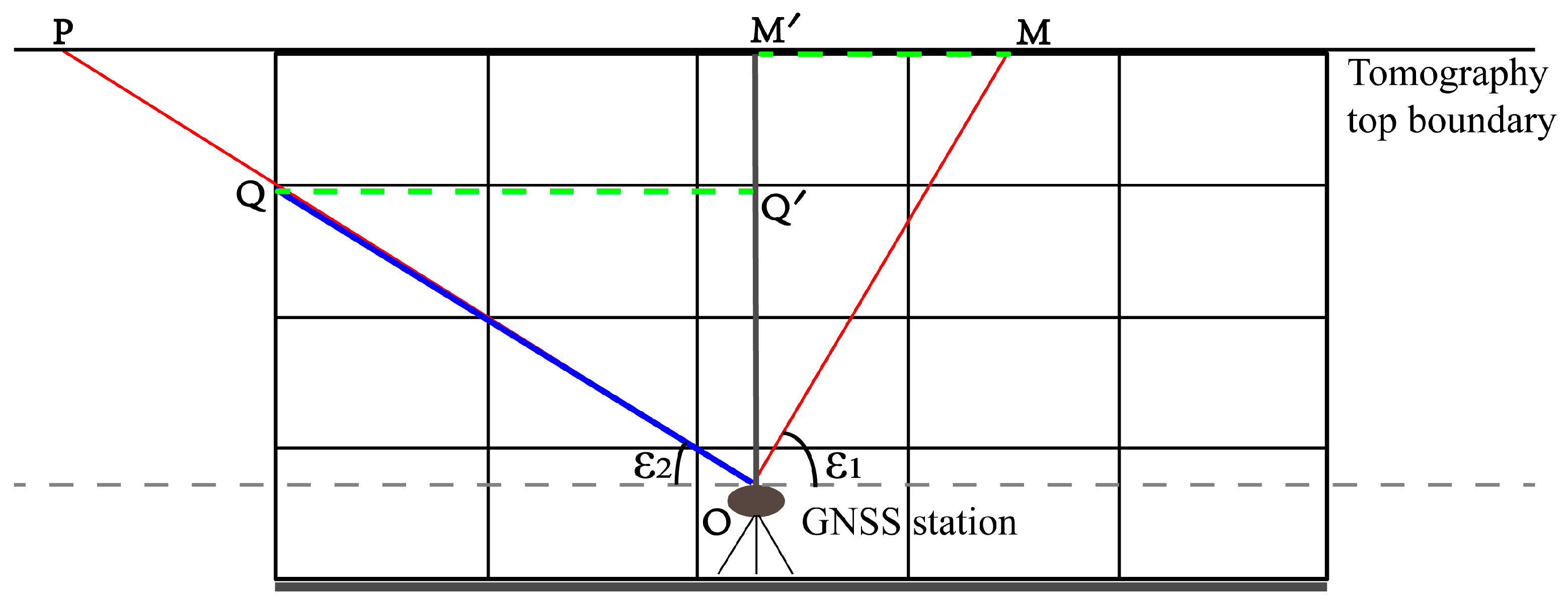
2.2. Dynamicity of the Tomography Top Boundary

The top boundary serves as a key factor for the GNSS water vapor tomography model. On the one hand, signals are classified into two categories (top and side signals) according to the positional relationship between themselves and the top boundary. It is worth noting that a higher top boundary leads to a lower number of top rays in the traditional tomography model, according to Chen and Liu [36]. On the other hand, redundant voxels where the WVD is close to zero will be introduced into the tomography system with an increasing top boundary. As a consequence, it is essential to identify an appropriate tomography top boundary to utilize more signals and avoid unnecessary voxels.

Water vapor, having an approximately exponential decreasing trend with altitude, is considered to be a criterion for determining the top boundary. In Yao and Zhao [14], the principle that a certain height with a WVD of less than 0.2 g/m³ can be considered as the top boundary of the tomography model is proposed.

In this study, the idea of determining the optimal tomography top boundary based on the water vapor vertical distribution derived from 30 years (1989–2018) of radiosonde data at Hong Kong King Park station (114.17°E, 22.31°N) is introduced. Accordingly, the water vapor profiles of different months in Hong Kong are shown in Figure 1.

It can be seen that the distribution trend of water vapor in the atmosphere varies greatly in different seasons. Evidently, the optimal top boundary in summer and autumn is higher than that in spring and winter. The mean height values of the tomography top boundary for the four seasons (spring corresponding to March to May, summer corresponding to June to August, autumn corresponding to September to November, and winter corresponding to December to February) are approximately 10.2, 10.9, 10.6, and 9.6 km, respectively. As a consequence, the tomography top boundary changes in different seasons, even for the same region, which can be deduced from this research. What is more, the dynamic top boundary of the tomography area, particularly in regions with complex weather conditions, should be determined from the local water vapor profiles in different months.

2.3. Construction of the Height Factor Model

In the three-dimensional voxel tomography model, the criterion for judging the availability of GNSS signals is where they puncture. In other words, only GNSS signals passing from the top boundary are selected as effective rays for the tomography system, and a number of side signals penetrating from the side of the tomography area are eliminated. Evidently, this behavior not only reduces the utilization of GNSS signals, but also generates more empty voxels in the three-dimensional model, which leads to a decline in the accuracy and stability of the tomographic results. Consequently, the HFM introduced in this paper will show the process of side signal modeling. The key for modeling side rays is the estimation of the SWD of inside signals, which is discussed in the HFM.

For the integral rays penetrating from the top boundary, their SWDs are calculated by using Equation (2). For instance, the SWD of signal $OM$ shown in Figure 2 is obtained by the ray path mapping of the ZWD of $M^{\prime }$, plus the gradient delay caused by the entire troposphere. Accordingly, the SWD of inside signals (e.g., signal $OQ$) can be estimated by the mapping of the ZWD of ray $O{Q}^{\prime }$ and the gradient delay as a result of the partial tropospheric impact. Therefore, we present the estimation of the SWD of inside signals in terms of two aspects—isotropic and anisotropic components—which are carefully discussed in the following two subsections.

2.3.1. Isotropic Component of SWD for Inside Signals

ZWD, considered as the isotropic component, is related to the water vapor above the GNSS station.

$$ZWD={{\displaystyle \int }}^{}{N}_{w}dh$$

(5)

Generally, Equation (5) is discretized into the following form in GNSS tomography [26]:

$$ZWD={{\displaystyle \sum }}_{i=1}^n{N}_w\left(h_i\right)·h_i,$$

(6)

where $N_w\left(h_i\right)$ represents the wet refractivity of the $ith$ layer and $h_i$ denotes the thickness of the $ith$ layer. The ZWD from the station to any height $h$ above the site can be correctly estimated using Equation (6). Therefore, we can establish the HFM to analyze the relationship between the height $h$ and the sectional ZWD, which may contribute to estimating the isotropic component of the SWD of inside signals.

Radiosonde data, preserving a high accuracy and optimal vertical resolution of meteorological parameters along the tropospheric column, are used to construct the HFM in this paper. The detailed steps are given below.

• The initial radiosonde data is encrypted to produce uniform data with a vertical resolution of 100 m and the water vapor density of the interpolation points is calculated using the cubic spline interpolation algorithm [37]. In the processing of radiosonde observations, the vertical resolution of radiosonde data at different remote sensing time is variable, i.e., the resolution of data in the lower layer is higher than that in the upper layer. It should be noted that observations with an even distribution can generate a more accurate fitting model. Therefore, the initial radiosonde data should first be encrypted to produce uniform data.
• The partial ZWD is computed from the surface to a certain height using Equation (6).
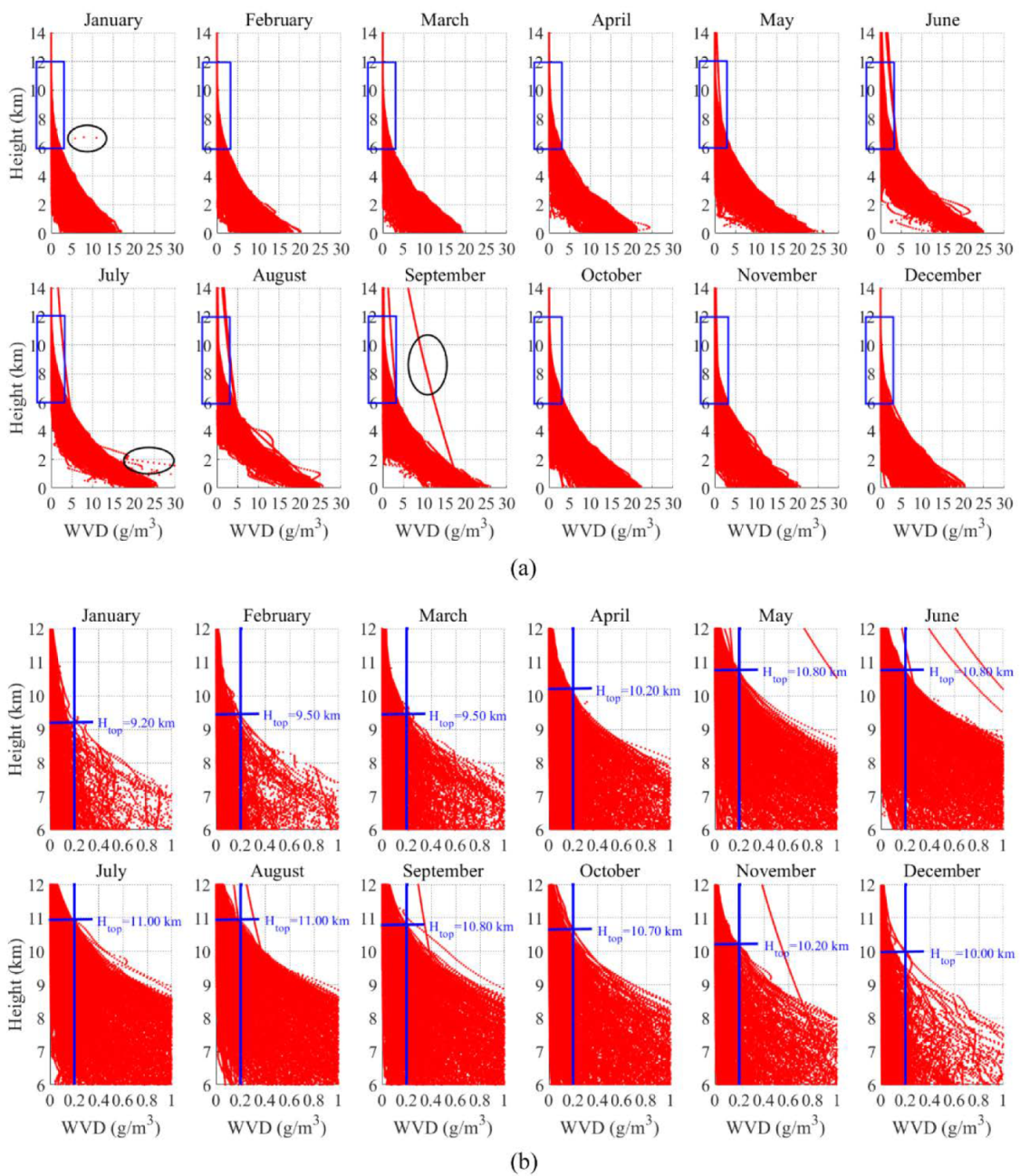
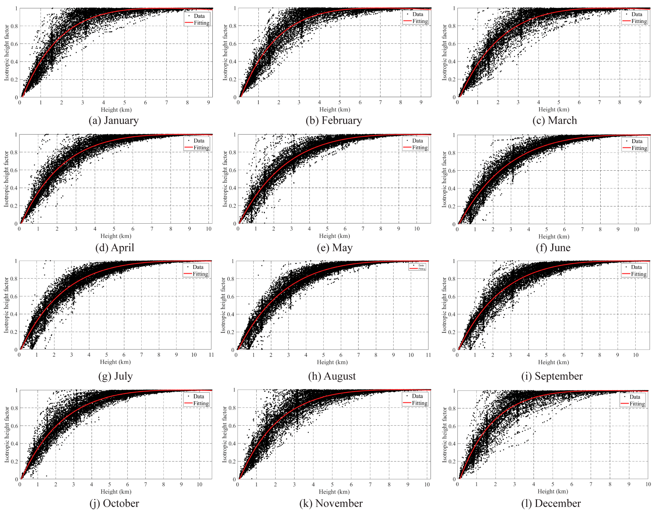
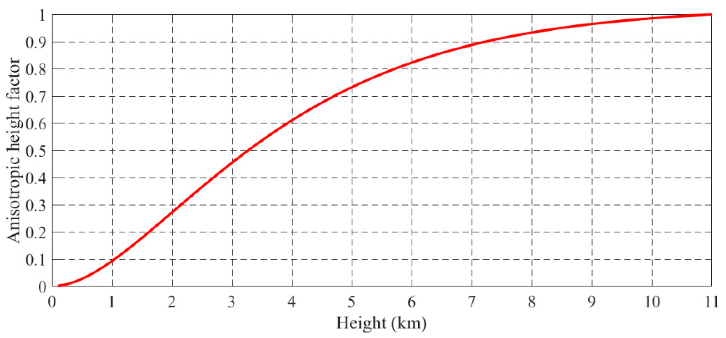
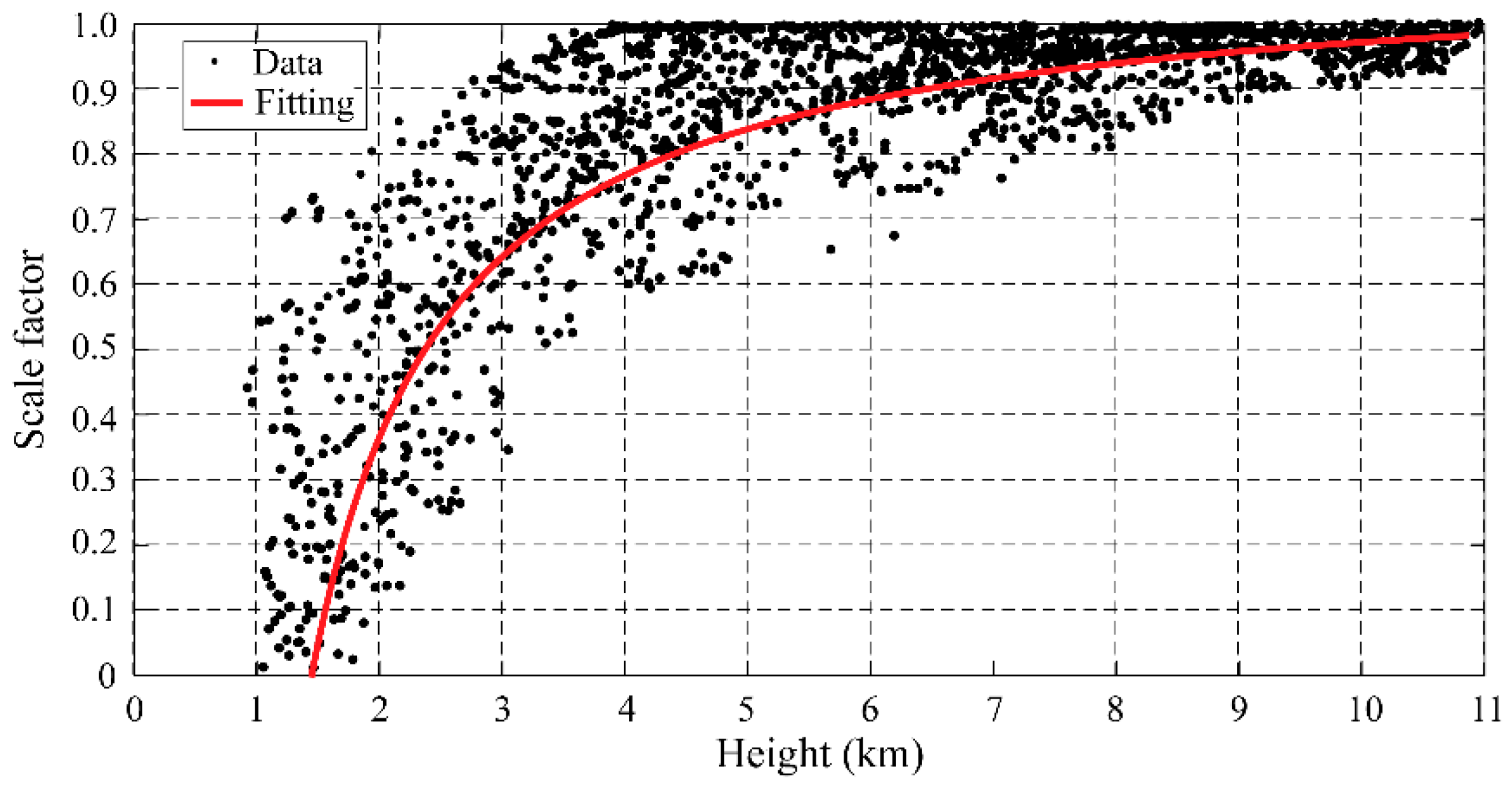
• The isotropic height factor ${\lambda }_{iso}\mathrm{is}\mathrm{defined}$, which represents the ratio between the partial content of ZWD and the total ZWD, as shown in Equation (7).

  $${\lambda }_{iso}\left(h\right)=\frac{ZW{D}_h}{ZW{D}_{total}},$$

  (7)

  where $ZW{D}_h$ denotes the partial ZWD from the surface to the height $h$, and $ZW{D}_{total}$ derived from the GNSS data is the total ZWD of the stations. Figure 3 shows the relationship between the isotropic height factor and the height based on the 30-year radiosonde data from different months in Hong Kong.
• The function relationship between the ${\lambda }_{iso}\left(h\right)$ and $h\mathrm{is}\mathrm{analyzed}$. In view of the variety of atmospheric water vapor, owing to the fact that the radiosonde balloon in Hong Kong is launched twice a day, at 00:00 UTC and 12:00 UTC, the radiosonde data cannot provide sufficient observations for daily-scale analysis. In addition, according to the periodic characteristics of ZTD and precipitable water vapor (PWV) [1,38], the relationship between the isotropic height factor and the height using 30 years of radiosonde data from 12 months is presented in Figure 3. Besides, the long-term trends of the isotropic height factor will not have an important impact on the tomography results. On the other hand, the wet refractivity water vapor decreases exponentially with height in the troposphere, and it is found from Equation (7) that the isotropic height factor ${\lambda }_{iso}$ is related to the wet refractivity in the zenith direction. In the work of Yao and Zhao [14], Zhao et al. [39], and Zhao et al. [27], a similar scale factor or truncation factor $\lambda$ is introduced, the trend of which changes with the height, as analyzed based on the exponential relationship in all three studies.
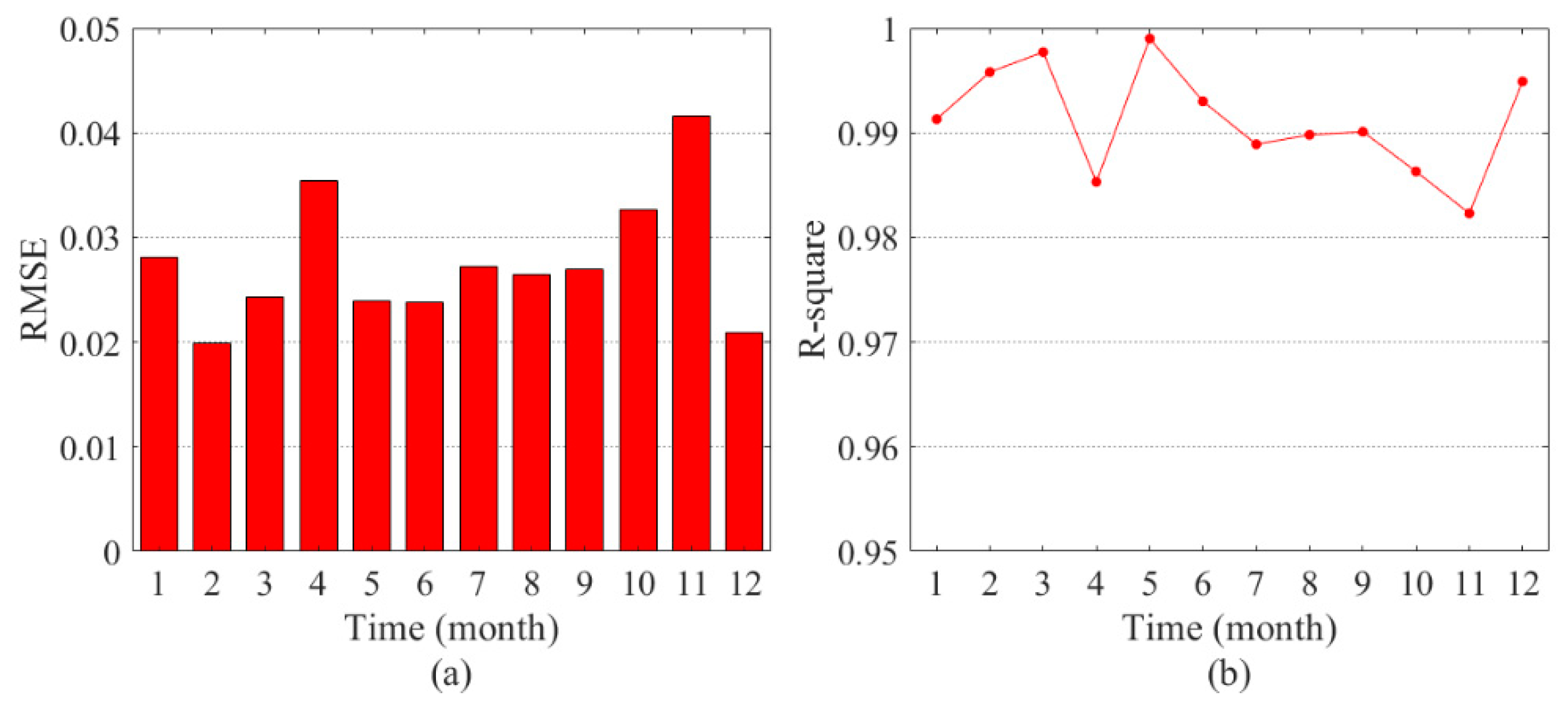
• Accordingly, the HFM is established as follows:

  $${\lambda }_{iso}\left(h\right)=a_1·e^{b_1·h}+a_2·e^{b_2·h},$$

  (8)

  where $a_1$, $b_1$, $a_2$, and $b_2$ represent the coefficients of the HFM, which are determined by least-squares fitting [27]. It should be noted that the different weather conditions during the 30 years are not classified, which may have an impact on obtaining the SWV of side signals and needs to be analyzed in future work.

Table 1. The optimal coefficient of the HFM for each month.

Month	${\mathit{a}}_1$	${\mathit{b}}_1$	${\mathit{a}}_2$	${\mathit{b}}_2$
January	1.093	−0.044	−0.184	−1.305
February	1.090	−0.042	−0.176	−1.351
March	1.122	−0.053	−0.220	−1.155
April	1.132	−0.060	−0.213	−1.133
May	1.117	−0.048	−0.206	−1.054
June	1.181	−0.070	−0.264	−0.911
July	1.089	−0.041	−0.153	−1.126
August	1.121	−0.051	−0.191	−1.019
September	1.088	−0.040	−0.158	−1.165
October	1.119	−0.053	−0.199	−1.130
November	1.089	−0.042	−0.172	−1.255
December	1.053	−0.026	−0.125	−1.516

shows the optimal coefficient for each month. Furthermore, the conclusion that the root mean square error (RMSE) of the 12 months of fitting results is less than 0.05 and the R-square representing the quality of the fitting results is greater than 0.98 can be inferred from Figure 4. It should be noted that the closer R-square gets to 1, the better the fitting results are [14]. Consequently, the isotropic component of SWD for inside signals could be accurately calculated using the HFM, as shown in Equation (9).

$$SW{D}_{isotropic}={\lambda }_{iso}\left(h\right)·m{f}_w\left(\epsilon \right)·ZW{D}_{zenith}$$

(9)

2.3.2. Anisotropic Component of SWD for Inside Signals

Gradient delays, characterizing the anisotropic water vapor distribution, have been intensively studied by a large number of scholars in VLBI analysis [28,32,33]. In the deduction of Boehm and Schuh [32], the two gradients mentioned above are obtained from the vertical integral of the water vapor refractivity gradient with height:

$$G_{\alpha }={10}^{-6}·{{\displaystyle \int }}_0^{H_{top}}{N}_{\alpha }\left(h\right)hdh,$$

(10)

where $\alpha$ denotes the azimuth direction (e.g., $NS$ or $EW$), $N_{\alpha }\left(h\right)$ is the water vapor refractivity gradient at height $h$, and $H_{top}$ represents the top of the troposphere in the integration.

Besides, the prevailing assumption that the refractivity gradient decreases exponentially with height was proposed in the work of Chen and Herring [33].

$$\frac{N_{\alpha }\left(h\right)}{N_S}=e^{-\frac{h}{H_{scale}}},$$

(11)

where $N_S$ is the refractivity gradient at the surface and $H_{scale}$ denotes the scale height of the neutral atmosphere, with a value of approximately 2 km, according to the local ground meteorological data [40]. The integral of Equation (10) can be written with the following expression:

$$G_{\alpha }\left(h\right)={10}^{-6}{N}_S\left[H_{scale}^2+e^{-\frac{H_{top}}{H_{scale}}}·\left(-H_{scale}^2-H_{top}·H_{scale}\right)\right].$$

(12)

In this section, an analysis of the gradient delay between the integral signal (e.g., $OP$ in Figure 2) and inside signal (e.g., $OQ$ in Figure 2) is performed. The anisotropic gradient delay of signal $OP$ and $OQ$ can be calculated with Equation (2).

$$\Delta L_G^{OP}=m{f}_g\left(\epsilon \right)·\left(G_{NS}^{OP}·\cos \left(\alpha \right)+G_{EW}^{OP}·\sin \left(\alpha \right)\right),$$

(13)

$$\Delta L_G^{OQ}=m{f}_g\left(\epsilon \right)·\left(G_{NS}^{OQ}·\cos \left(\alpha \right)+G_{EW}^{OQ}·\sin \left(\alpha \right)\right),$$

(14)

where $\Delta L_G^{OP}$ and $\Delta L_G^{OQ}$ represent the anisotropic component of SWD of integral signal $OP$ and inside signal $OQ$, respectively, and $m{f}_g\left(\epsilon \right)=\frac{1}{\sin \left(\epsilon \right)·\tan \left(\epsilon \right)+0.003}$ denotes the horizontal gradient mapping function [33]. $G_{\alpha }^{OP}$ and $G_{\alpha }^{OQ}$, the wet gradients of two rays, can be computed by using Equation (12). Therefore, we can define the anisotropic height factor ${\lambda }_{aniso}$ to estimate the relationship between the $\Delta L_G^{OP}$ and $\Delta L_G^{OQ}$.

$${\lambda }_{aniso}\left(h_{O{Q}^{\prime }}\right)=\frac{\Delta L_G^{OQ}}{\Delta L_G^{OP}}=\frac{H_{scale}^2+e^{-\frac{h_{O{Q}^{\prime }}}{H_{scale}}}·\left(-H_{scale}^2-h_{O{Q}^{\prime }}·H_{scale}\right)}{H_{scale}^2+e^{-\frac{H_{top}}{H_{scale}}}·\left(-H_{scale}^2-H_{top}·H_{scale}\right)},$$

(15)

where $h_{O{Q}^{\prime }}$ and $H_{top}$ represent the height of the zenith projection of the slant path $OQ$ and $OP$ along the zenith, respectively. During the tomography periods in Hong Kong in August 2017, the tomography top boundary $H_{top}$ was determined to be 11 km from Figure 1, and $H_{scale}$ was set to 2 km, according to the ground meteorological data in Hong Kong. Therefore, the anisotropic height factor ${\lambda }_{aniso}\left(h_{O{Q}^{\prime }}\right)$ only has a functional relationship with height $h_{O{Q}^{\prime }}$. For instance, $h_{O{Q}^{\prime }}$ increases equidistantly from 0 to 11 km with the interval of 0.1 km, and the corresponding ${\lambda }_{iso}\left(h_{O{Q}^{\prime }}\right)$ could be calculated by Equation (15). With the sample data of $h_{O{Q}^{\prime }}$ and ${\lambda }_{iso}\left(h_{O{Q}^{\prime }}\right)$, the red curve in Figure 5 could be drawn.

Similarly, the anisotropic gradient delay of inside signals can be written in the following equation:

$$SW{D}_{anisotropic}={\lambda }_{aniso}\left(h\right)·\Delta L_G^{integral},$$

(16)

where $SW{D}_{anisotropic}$ is the anisotropic delay component of inside signals on the same ray path with the observed signal, and $\Delta L_G^{integral}$ represents the anisotropic delay component of the observed signal.

As a consequence, the SWD of inside signals can be computed with

$$\begin{array}{cc}SW{D}_{inside}\hfill & =SW{D}_{isotropic}+SW{D}_{anisotropic}\hfill \\ \hfill & ={\lambda }_{iso}\left(h\right)m{f}_w\left(\epsilon \right)ZW{D}_{total}+{\lambda }_{aniso}\left(h\right)\Delta L_G^{integral}\left(\epsilon ,\alpha \right).\hfill \end{array}$$

(17)

In this work, $ZW{D}_{total}$ and $\Delta L_G^{integral}\left(\epsilon ,\alpha \right)$. were calculated with the ZTD, $G_{NS}$, and $G_{EW}$, respectively, which were estimated by GAMIT/GBLOK(v.10.7) [41]. The SWD of inside signals could be converted into SWV using Equation (3) for the improved tomography model.

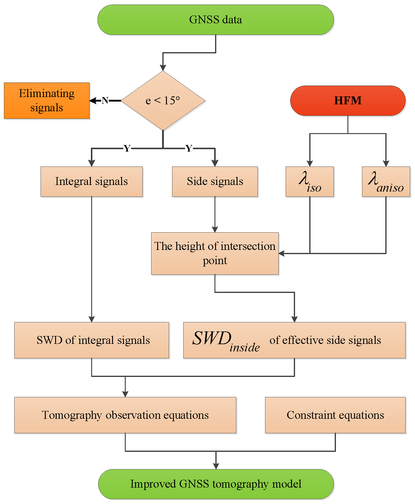
3. Modeling the GNSS Observations with the Proposed HFM

In common GNSS tomographic models, only GNSS signals passed from the top boundary are considered as effective observations for the tomographic model [10]. In this section, an improved GNSS tomography algorithm based on HFM is introduced, as shown in Figure 6. The process of GNSS tomography equations using integral signals and inside signals is discussed, respectively. The horizontal and vertical constraints are also described in detail.

Additionally, in most tomography models, to obtain as many effective signals as possible, the influence of the elevation angle is neglected. However, signals which enter the neutral atmosphere at low elevation angles ($\mathrm{e}<15°$) are significantly affected by atmospheric bending, according to Möller and Landskron [38]. As the bending effect is not modeled by the tomographic algorithms, rays with an elevation angle below 15° are first eliminated.

3.1. Constructing Tomography Observation Equations Using Integral Signals

To reconstruct the three-dimensional water vapor field, the tomographic area is divided into a number of uniformly distributed voxels over a GNSS network. Generally, the WVD within a voxel, assumed to be constant for a tomographic epoch, is estimated as one parameter. GNSS signals, from the GNSS sites to the top or side boundary of the tomographic region, provide the distance traveled in each voxel. Accordingly, Equation (1) can be discretized to a linear equation with the following form:

$$SW{V}_j={\displaystyle \sum }_{i=1}^{n_j}{d}_{ij}·x_i.$$

(18)

Note that the SWD of GNSS rays was converted into SWV using Equation (3) for the tomographic system. $d_{ij}$ denotes the distance traveled by the $j$th ray in the $i$th voxel, whose WVD is represented by $x_i$. $n$ is the total number of voxels intersected by the ray $j$.

For integral signals, passing from the top boundary of the tomography area, the observation equation can be written in matrix notation:

$$SW{V}_{integral}=A_{integral}·X,$$

(19)

where $SW{V}_{integral}$ is the observation vector of integral signals and $A_{integral}$. represents the observation matrix, including the distance traveled in each voxel. $X$ denotes the unknown vector for the three-dimensional tomographic model.

3.2. Constructing Tomography Observation Equations Using Inside Signals

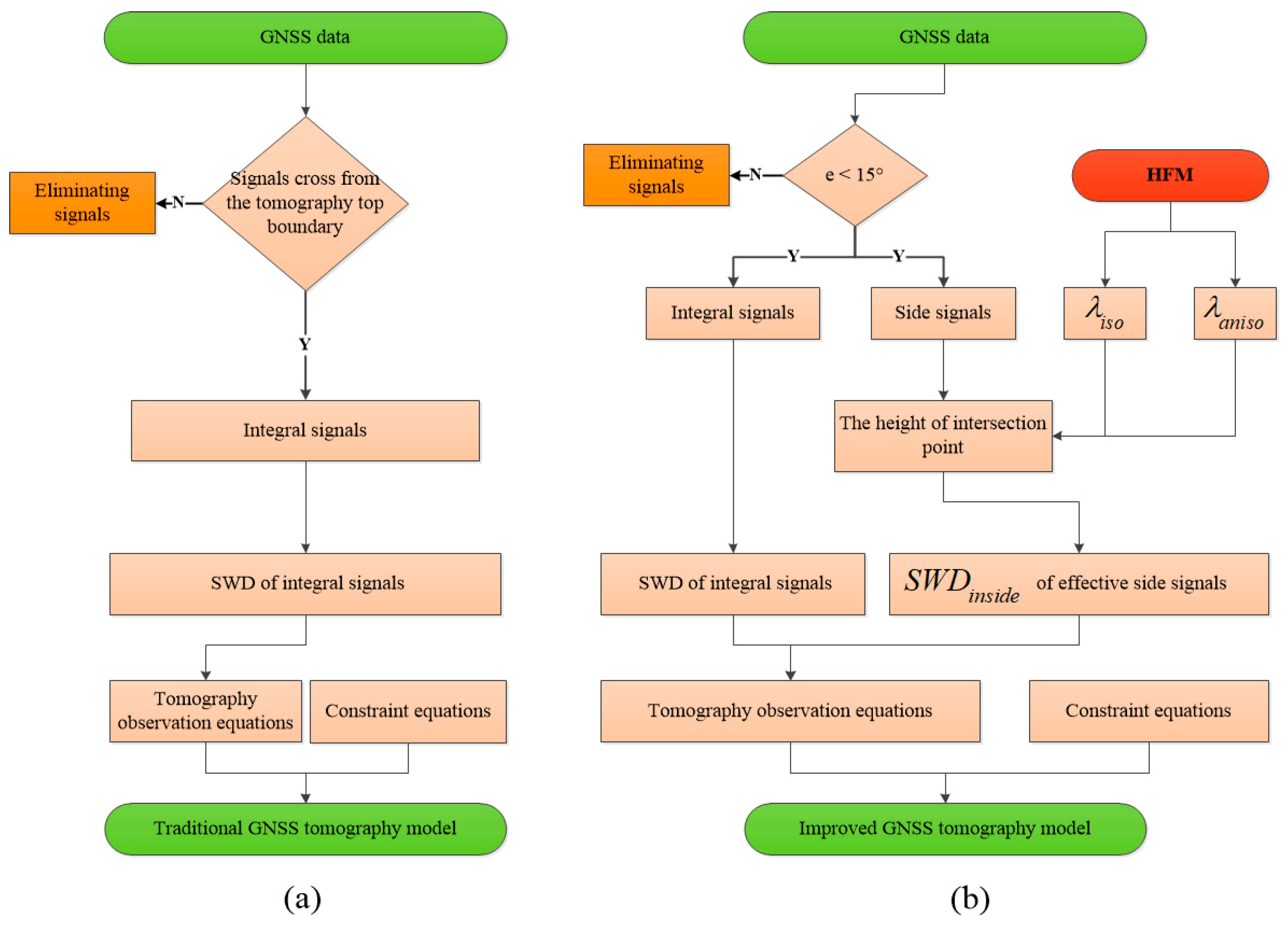
For inside signals, penetrating from the side of the tomography area, the SWD should first be estimated by HFM. The specific steps of computing the $SW{D}_{inside}$ are as follows:

• The ZTD and horizontal gradients of effective side signals (e.g., OP in Figure 2) are estimated using GAMIT/BLOCK. The ZWD, north, and east wet gradients can be extracted from the estimated values [7];
• The height $h_{inter}$ of the intersection point between the effective side signals and the side face of the tomographic area is calculated. The ${\lambda }_{iso}\left(h_{inter}\right)$ and ${\lambda }_{aniso}\left(h_{inter}\right)$ are estimated by Equations (8) and (15), respectively. Then, the SWD of inside signals can be calculated using Equation (17);
• The distance information of inside signals is obtained with the ray-tracing method [42], and the unknowns are related to the inside observations by the following equation:

  $$SW{V}_{inside}=A_{inside}·X,$$

  (20)

  where $SW{V}_{inside}$ is the observation vector of inside signals and $A_{inside}$ represents the observation matrix derived from inside signals.

3.3. Constructing Tomography Constraint Equations

Although side signals with an elevation angle greater than 15° are utilized, there are still some empty voxels in the three-dimensional tomographic model [10]. Usually, spatial constraints are introduced in the tomography system to relieve the ill-conditioned problem.

The following horizontal constraint, assuming that the WVD of a voxel is equal to the weighted mean of the WVD of the surrounding voxels in the same layer [7], is applied for the tomography system:

$$x_i=w_{1j}{x}_1+w_{2j}{x}_2+\dots +w_{i-1j}{x}_{i-1}+w_{i+1j}{x}_{i+1}+\dots +w_{n_h j}{x}_{n_h},$$

(21)

where $n_h$ represents the number of voxels in a certain layer and $x_i$ is the WVD of the $i$th voxel. $w_{ij}$ denotes the horizontal weighted coefficient of the $j$th surrounding voxel in this layer corresponding to the $i$th voxel. The Gauss weighting function proposed in Song et al. [21] is introduced to calculate the coefficients:

$$w_{ij}=\frac{e^{-\frac{d_{ij}^2}{2{\sigma }^2}}}{{{\displaystyle \sum }}_{i=1}^{n_h}{e}^{-\frac{d_{ij}^2}{2{\sigma }^2}}},$$

(22)

where $d_{ij}$ is the distance between the $i$th voxel and the $j$th surrounding voxel. $\sigma$ represents the smoothing factor and is 1.5 times longer than the horizontal length of voxels [21].

In addition, the WVD can be described by exponential decay with an increasing height [43]:

$$x_{k+1}=e^{\frac{h_k-h_{k+1}}{H_{scale}}}·x_k,$$

(23)

where $x_k$ and $h_k$ denote the WVD and height of the $k$th layer, and $H_{scale}$ is the scale height mentioned in Equation (11).

As a result, the final tomographic system equations can be written as follows:

$$\left(\begin{array}{c}\begin{array}{c}{P}_{integral}·Y_{integral}\\ P_{inside}·Y_{inside}\end{array}\\ \begin{array}{c}0\\ 0\end{array}\end{array}\right)=\left(\begin{array}{c}\begin{array}{c}{P}_{integral}·A_{integral}\\ P_{inside}·A_{inside}\end{array}\\ \begin{array}{c}{P}_{hz}·A_{hz}\\ P_{vert}·A_{vert}\end{array}\end{array}\right)·X,$$

(24)

where $Y_{integral}$ and $Y_{inside}$ are the observation vector of the integral signals and side signals, respectively. Similarly, both $A_{integral}$ and $A_{inside}$ represent the observation matrix, including the distance traveled in each voxel. The weighting matrix was also imposed on the tomographic observation equations. $P_{integral}$ and $P_{inside}$, representing the weighting matrix of integral and inside rays, have a functional relationship with the elevation angle of the signal path [26]. However, for the weighting matrix of horizontal and vertical constraints, $P_{hz}$ and $P_{vert}$, having a similar impact on voxels, are by default the identity matrix [26].

Due to the morbidity of the coefficient matrix, the Algebraic Reconstruction Technique (ART), with the advantages of simple iteration and fast convergence [10,44], is introduced to solve the tomography observation equations in this work.

4. Experiments and Results

In general, since voxels located on the side of the tomographic area do not travel by any ray, the water vapor density of these voxels can be estimated based on only constraint equations, which reduces the accuracy of the tomography solutions. The primary contribution of the side signals is to ensure that voxels not passed in the traditional model can be crossed, which allows the accuracy and stability of tomographic results to be improved. To test the HFM and evaluate the efficiency of side signals, four special experimental schemes were performed separately. Section 4.1 describes the implementation of the four experimental schemes; the contribution of the side signals to the tomography solutions is analyzed in Section 4.2. On the other hand, the existing improved model combining the side observations was reestablished using the GNSS data [14], and is compared to the proposed HFM in Section 4.3.

It should be noted that when assessing the accuracy of tomography solutions, the vertical profiles obtained from radiosonde were used as reference values. Although the radiosonde data has been made use of to calculate the isotropic height factor, its main contribution is to provide the vertical distribution characteristics of atmospheric water vapor, not to participate in the tomographic processing. For instance, the tomographic time was set to August 2017, according to the HFM, and the optimal tomography top boundary was set to 11 km. Additionally, the height factor model ${\lambda }_{iso}\left(h\right)=1.121·e^{-0.051h}-0.191·e^{-1.019h}$ was applied to calculate the isotropic height factor. Consequently, only GNSS observations went sent to the tomography system as input information for reconstructing the three-dimensional water vapor field, which shows that the proposed HFM does not interfere with the accuracy assessment of tomography results.

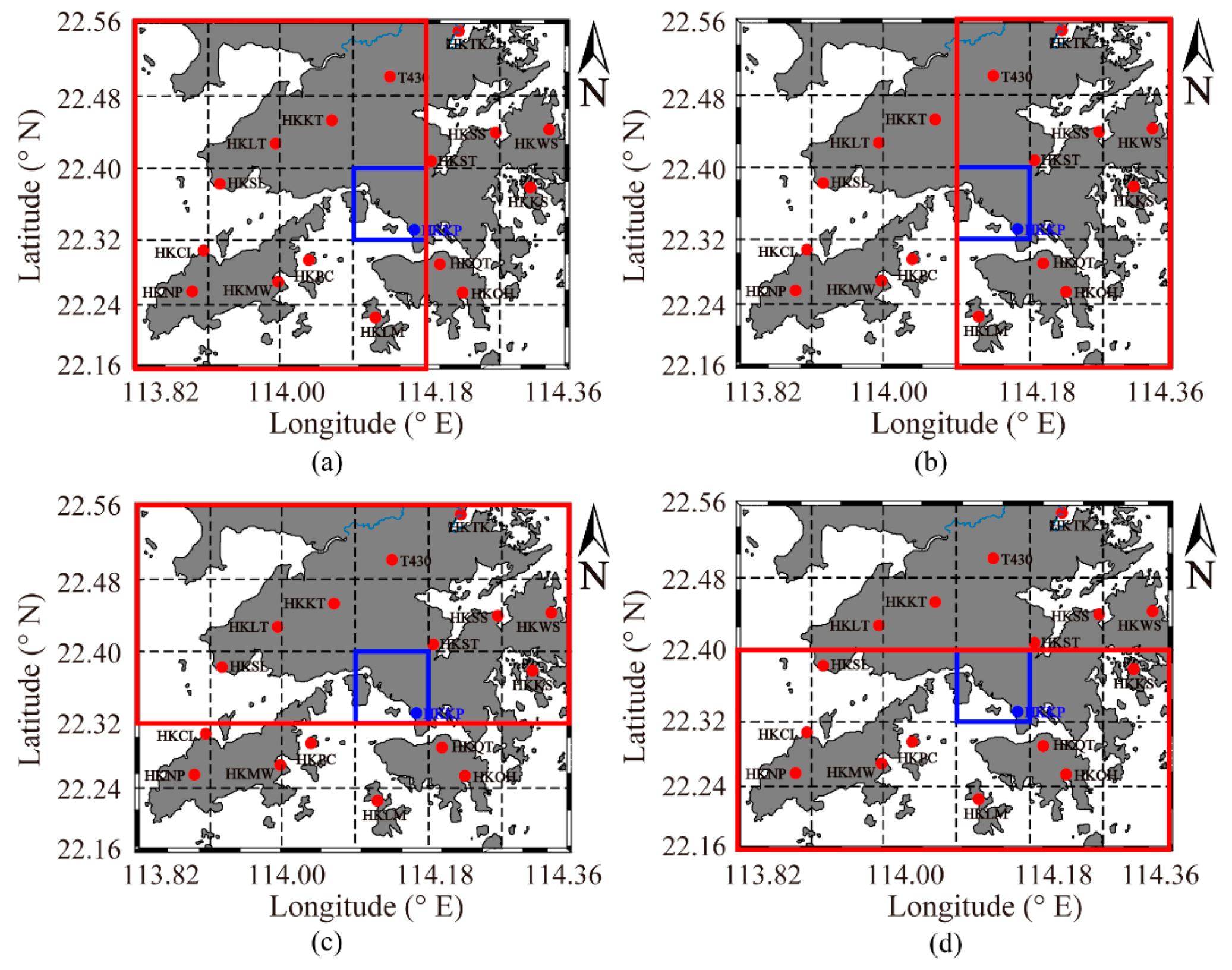
4.1. Experimental Schemes

The GNSS data with the sampling rate of 30 s from 17 stations (red dot in Figure 7) provided by the Hong Kong Satellite Positioning Reference Station Network (SatRef) were processed using GAMIT/GLOBK (v.10.7). In the processing, the four International GNSS Service (IGS) stations (BJFS station, HKWS station, LHAZ station, and SHAO station) were introduced. The ZTD and the gradient delay were estimated with the time resolution of 5 min, which was sufficient to reveal the variation characteristics of water vapor. The Saastamoinen model was set as the expression for the ZHD [45], and Vienna Mapping Function 1 (VMF1) was used for calculating the SWDs [46]. In addition, the post-fit residuals calculated by GAMIT/GLOBK exceeding 2.5 times the standard deviation were removed [47]. The 30-year radiosonde observation data was obtained from the King’s Park Meteorological Station (HKKP, the blue dot in Figure 7a). The research area of the tomography model spanned from 113.82°E to 114.36°E and 22.16°N to 22.56°N. Moreover, the horizontal resolution was 0.09° in longitude and 0.08° in latitude, as shown in Figure 7a. In the current tomography studies based on the Hong Kong SatRef, about a month of GNSS data and the radiosonde observations derived from the HKKP station were processed for modeling the tomography area [14,20,36,41]. Therefore, the experimentation time in this work was set as August 2017, i.e., day of year (DOY) 213–243, when Hong Kong was in the summer and there were more rainstorms. The tomography region was segmented into 15 nonuniform layers from 0 to 11 km (August top boundary determined in Figure 2) [14].

In the most common voxel-based tomography model, to assess the accuracy of tomographic results, water vapor profiles of the voxel columns (small blue rectangles in Figure 7b) where the radiosonde is located are compared with radiosonde-derived vertical profiles. However, the empty voxels are mainly distributed on the side of the three-dimensional tomographic model. Consequently, as shown in Figure 8, four special test schemes based on four different tomography areas (red boxes of Figure 8a–d) were implemented. The RS-voxels (the blue voxels, shown in Figure 7b, where the radiosonde is located) were placed on four boundaries of the tomographic region in the four schemes, for instance, RS-voxels on the east side (Figure 8a), RS-voxels on the west side (Figure 8b), RS-voxels on the south side (Figure 8c), and RS-voxels on the north side (Figure 8d).

Table 2. The range of the tomographic area and the number of voxels in the four schemes.

Scheme	Range	Voxel Division	Total Numbers
Scheme East	113.82°E~114.18°E; 22.16°N~22.56°N	$4\times 5\times 15$	300
Scheme West	114.09°E~114.36°E; 22.16°N~22.56°N	$3\times 5\times 15$	225
Scheme South	113.82°E~114.36°E; 22.32°N~22.56°N	$6\times 3\times 15$	270
Scheme North	113.82°E~114.36°E; 22.16°N~22.40°N	$6\times 3\times 15$	270

shows the accurate range of the tomographic area and the number of voxels in these four schemes.

In addition, to verify the accuracy and reliability of the HFM, two sub-groups of solutions were generated for the four schemes; one only used the rays travelling from the top boundary, while the others combined both rays passing from the top and side boundaries. It should be noted that if the effective observations from the HKSC station are included, the data is not consistent with the signal distribution of the general tomographic model. In addition, due to the RS-voxels always being crossed by rays in the four schemes, the benefit of the side signal for improving the accuracy of the water vapor density of the un-punctured voxels cannot be evaluated accurately. Therefore, all observations from HKSC station were excluded in the four schemes.

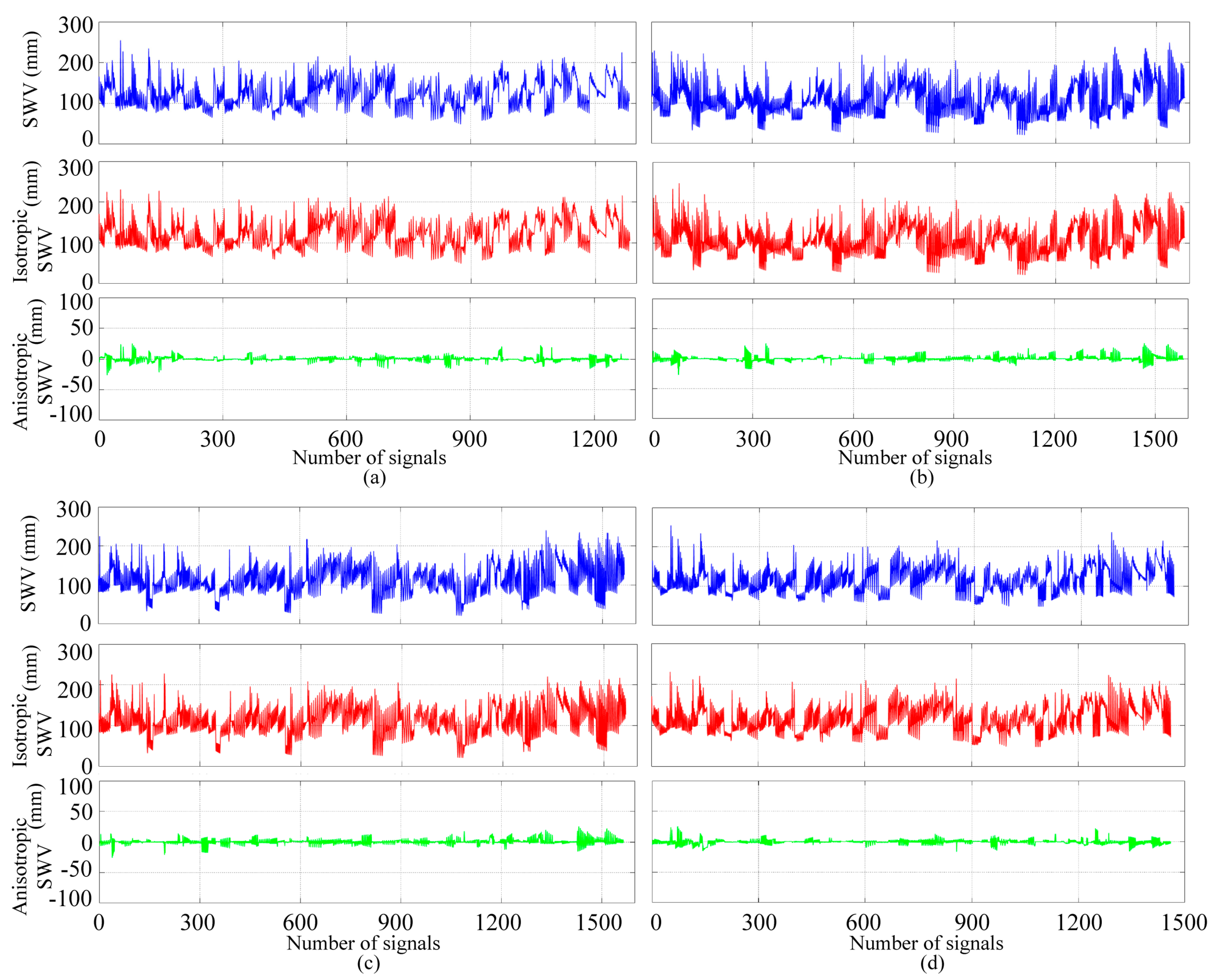
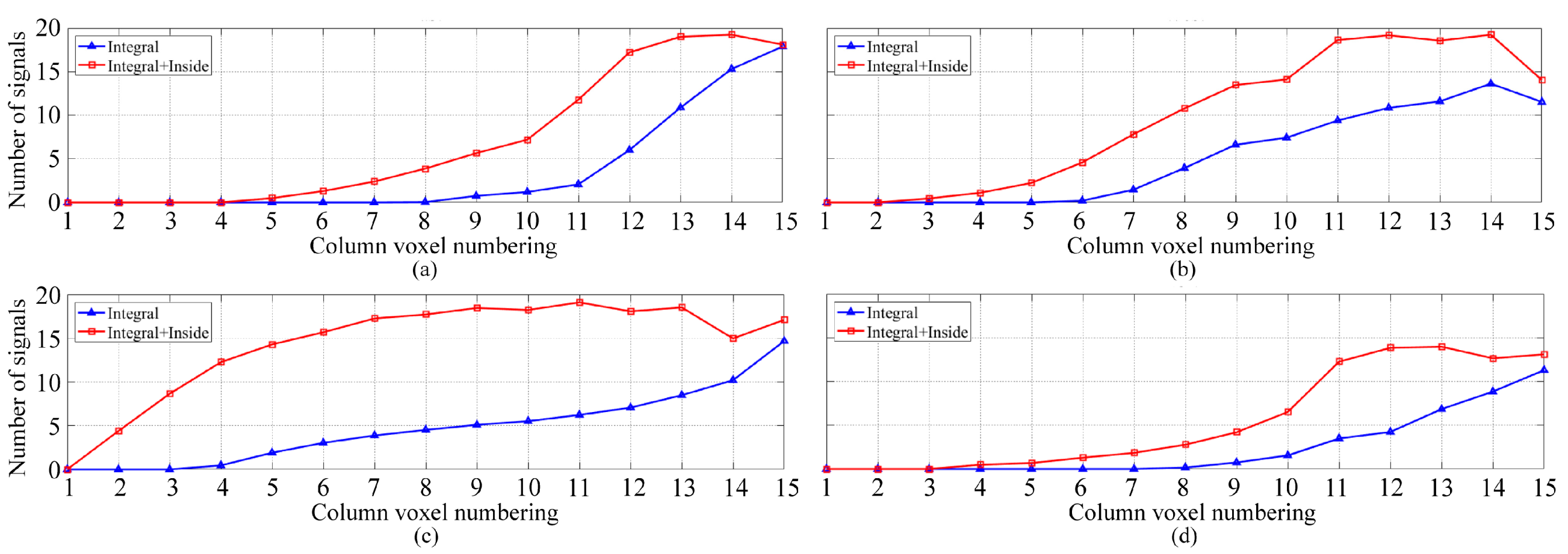
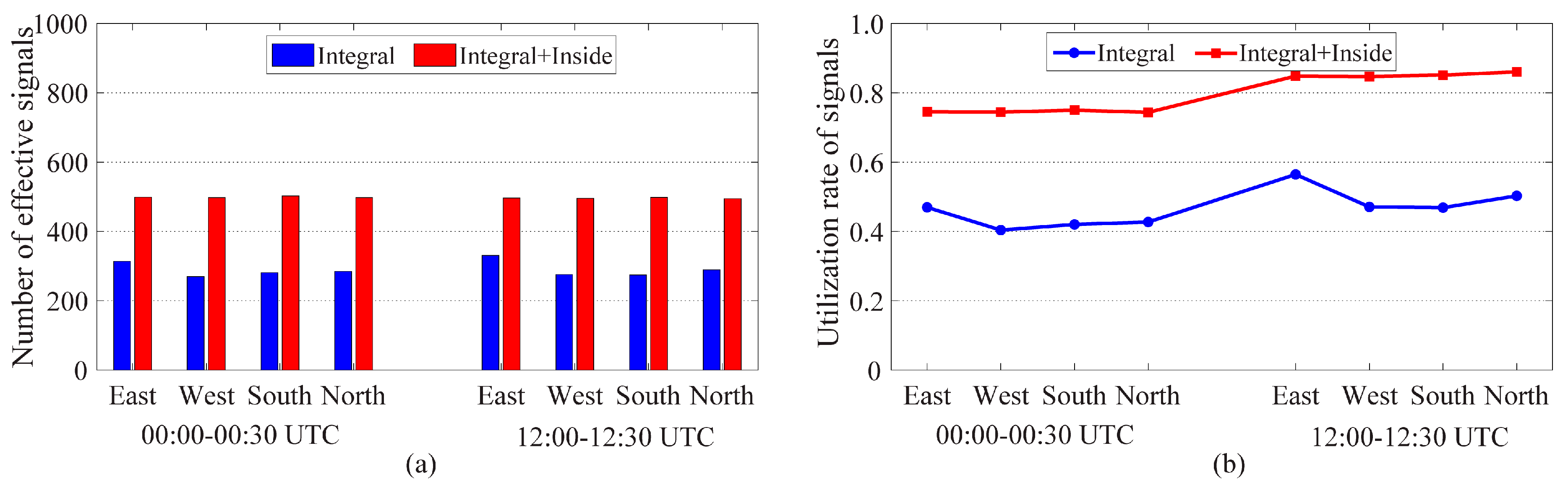
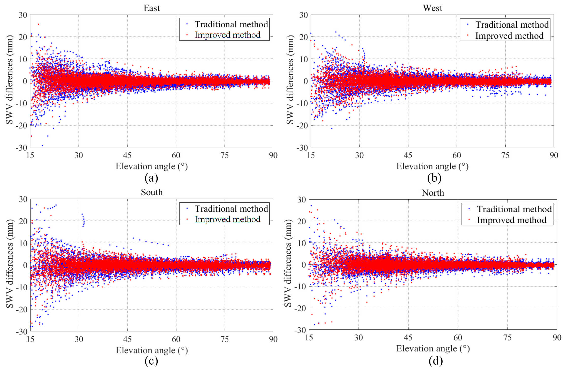
4.2. Contribution Analysis of the Side Signals

The isotropic and anisotropic SWV values of inside signals were first estimated by the HFM, as listed in Figure 9. A slight consistency between the total SWV and the isotropic one can be noticed from the four sub-figures. In contrast, the anisotropic parts were inconsistent with the totals and only accounted for an average of 2.31%, 2.56%, 2.61%, and 2.25% of the corresponding total component in the four schemes, which reveals that the isotropic portion has a more marked significance than the anisotropic portion in estimating the SWV value of the inside signals. However, the latter, with a value of approximately 20 mm for certain rays, is also important.

Furthermore, we developed a detailed analysis of the number of rays crossing from the RS-voxel columns. Figure 10 demonstrates the benefit of absorbing inside signals into the traditional tomography model. Evidently, in the East, West, and North schemes, no signals passed from the voxel from layer 1 to layer 8 in the general tomography model, while only the first four layers of voxels were not penetrated by rays in the improved model. As far as the South scheme is concerned, it is noticeable that the RS-voxel columns were all passed by GNSS rays in the optimized model, except for the voxel on the first layer. The number of penetrated signals tripled for voxels from 2 to 11 layers when adding the inside rays.

The average number of effective rays and the mean signal utilization rate for the traditional model and optimized model during the tomographic period are also compared in Figure 11, where the histogram shows the number of signals and the line chart represents the signal utilization rate. The former refers to the 31-day average number of GNSS rays selected in the tomography model during the two epochs. Similarly, the latter represents the 31-day mean utilization rate of the number of rays used in the equations out of the total number of GNSS signals in each tomography epoch. Because the GNSS rays with an elevation angle below 15° were eliminated, the mean utilization rate of integral signals and inside ones was about 80% in the four schemes. With side signals absorbed into the tomography system, the mean effective rays increased by 32.33%, whereas the average utilization rate of GNSS signals was enhanced by 33.42%, from 47.12% to 80.54%. In particular, the number of effective signals combining inside ones remained an approximative constant for any tomographic scheme, which enhanced the stability of the improved tomography model.

The three-dimensional WVD was reconstructed using the traditional method and the proposed approach, respectively. To assess the retrieval capabilities of the optimized tomographic model, the SWV differences between the observed SWV and reconstructed SWV from the three-dimensional tomographic water vapor field were calculated, and the SWV differences between the traditional method and the proposed approach were obtained, respectively. Figure 12 illustrates a comparison of the SWV differences between the two methods in the four schemes.

There is a noticeably similar tendency, in that the SWV differences of GNSS signals with an elevation angle larger than 45° are in the range of −5 to 5 mm, while those of rays with an elevation angle lower than 45° sharply increase with a decreasing elevation angle in all four schemes. As far as the comparison of SWV differences between the general and optimal tomography model is concerned, a remarkable improvement can be identified in the East scheme, West scheme, and South scheme, whereas the proposed method is slightly better than the traditional one in the North scheme. The same conclusion can also be deduced from

Table 3. Statistical results of the comparison of SWV between reconstructions and measurements for the four schemes (unit: mm).

Scheme	Data	RMSE	STD	Bias
Scheme East	Integral only	13.08	12.83	−0.33
	Integral+inside	9.97	9.49	−0.17
Scheme West	Integral only	12.05	11.55	−0.29
	Integral+inside	9.50	9.36	−0.25
Scheme South	Integral only	13.69	13.26	−0.25
	Integral+inside	11.09	10.64	−0.24
Scheme North	Integral only	10.46	10.39	−0.27
	Integral+inside	9.19	9.04	−0.14

, where the statistics, including the RMSE, standard deviation (STD), and bias, for the SWV differences from the four schemes are compared. The improvements of the combined observations with respect to only the integral one are 3.11/3.34, 2.55/2.19, 2.60/2.62, and 1.27/1.35 mm for the RMSE/STD in the four schemes, respectively. In the bias comparison, there is a visible advancement of the tomography solutions when inside signals are included.

In addition, the tomographic results derived from the general model and improved model were compared with radiosonde data at 00:00 UTC and 12:00 UTC, when the radiosonde data provided accurate water vapor profiles at different altitudes.

Table 4. The mean RMSE and STD for the conventional method and proposed method during the 31-day period from DOY 213 to DOY 243, 2017 (unit: g/m³).

Scheme	Data	RMSE	STD
Scheme East	Integral only	1.60	1.59
	Integral+inside	1.07	1.06
Scheme West	Integral only	1.62	1.61
	Integral+inside	1.12	1.08
Scheme South	Integral only	1.66	1.64
	Integral+inside	1.34	1.33
Scheme North	Integral only	1.63	1.61
	Integral+inside	1.13	1.11

lists the mean RMSE and STD of the tomography results retrieved from the integral signals and combined signals for August 2017. It can be observed that the tomography results are closer to the radiosonde data when the inside rays are absorbed. The improved tomography model displays a smaller RMSE than the conventional one in the four test schemes, with decreases of 33.12%, 30.86%, 19.27%, and 30.67% in the mean RMSE, and the approximate consistent decrease rate of the STD for the four schemes can also be computed from Table 4.

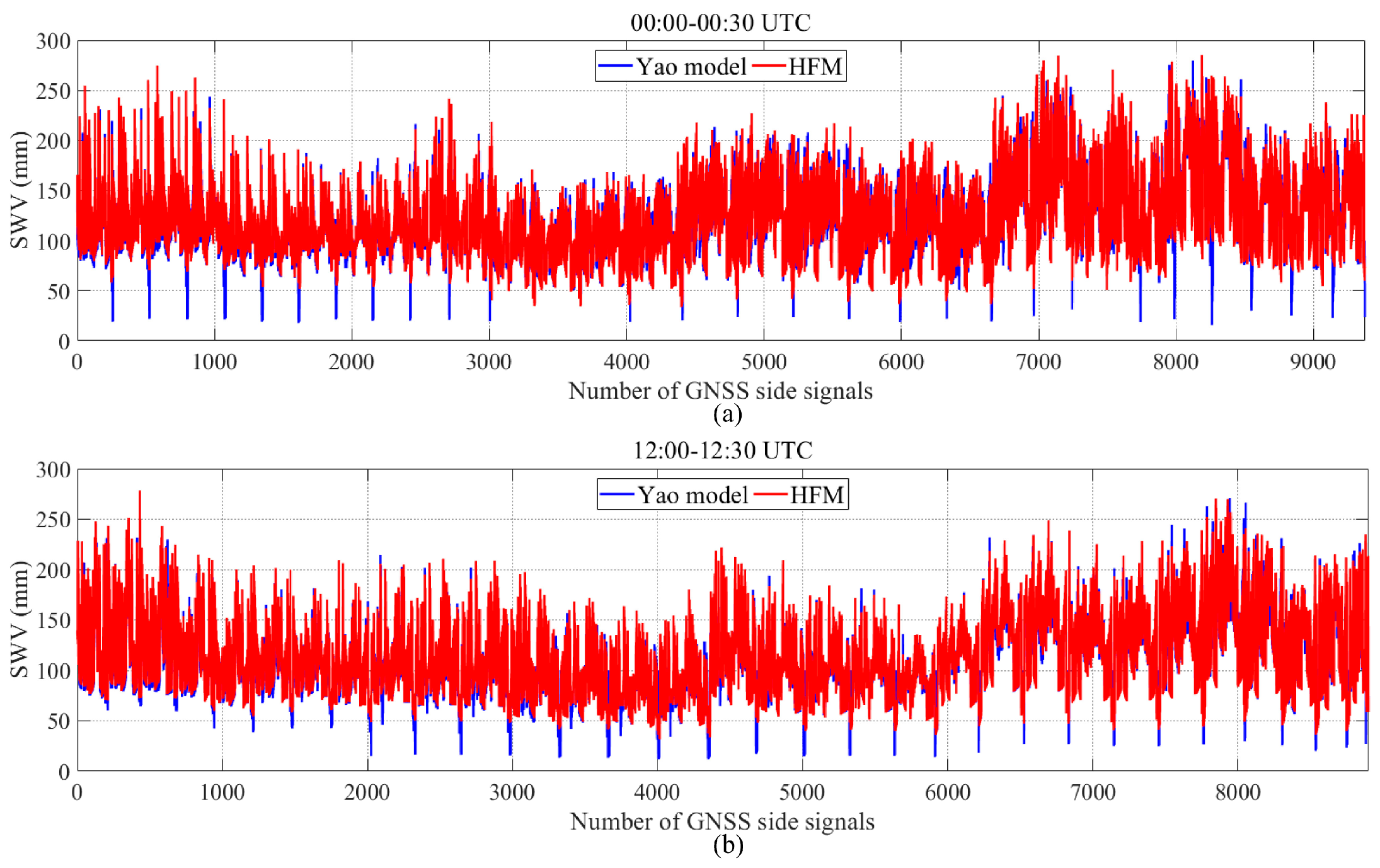
4.3. Comparison with the Existing Correction Model

In this section, the HFM in the current study is compared with the existing correction model in Yao and Zhao [14], which is named the Yao model in this work for convenience. In the Yao model, a similar exponential relationship between the scale factor and the height is established, as follows [14]:

$$\alpha =a+b·e^{\frac{1}{h}},$$

(25)

where $\alpha$ is the scale factor, and $a$ and $b$ represent the coefficients of the scale factor, respectively. $h$ denotes the height of the intersection point between the effective side signals and the side face of the tomography area.

To compare the performance of the HFM and Yao model in retrieving the three-dimensional water vapor field, three further schemes were designed for tomography modeling based on all GNSS station observations from the Hong Kong SatRef, in addition to the HKSC station. The tomographic region for the three schemes covers from 113.82°E to 114.36°E in longitude and 22.16°N to 22.56°N in latitude. Other tomographic model configurations, such as a horizontal and vertical resolution, are consistent with the four special experimental schemes. The three schemes in this section are as follows.

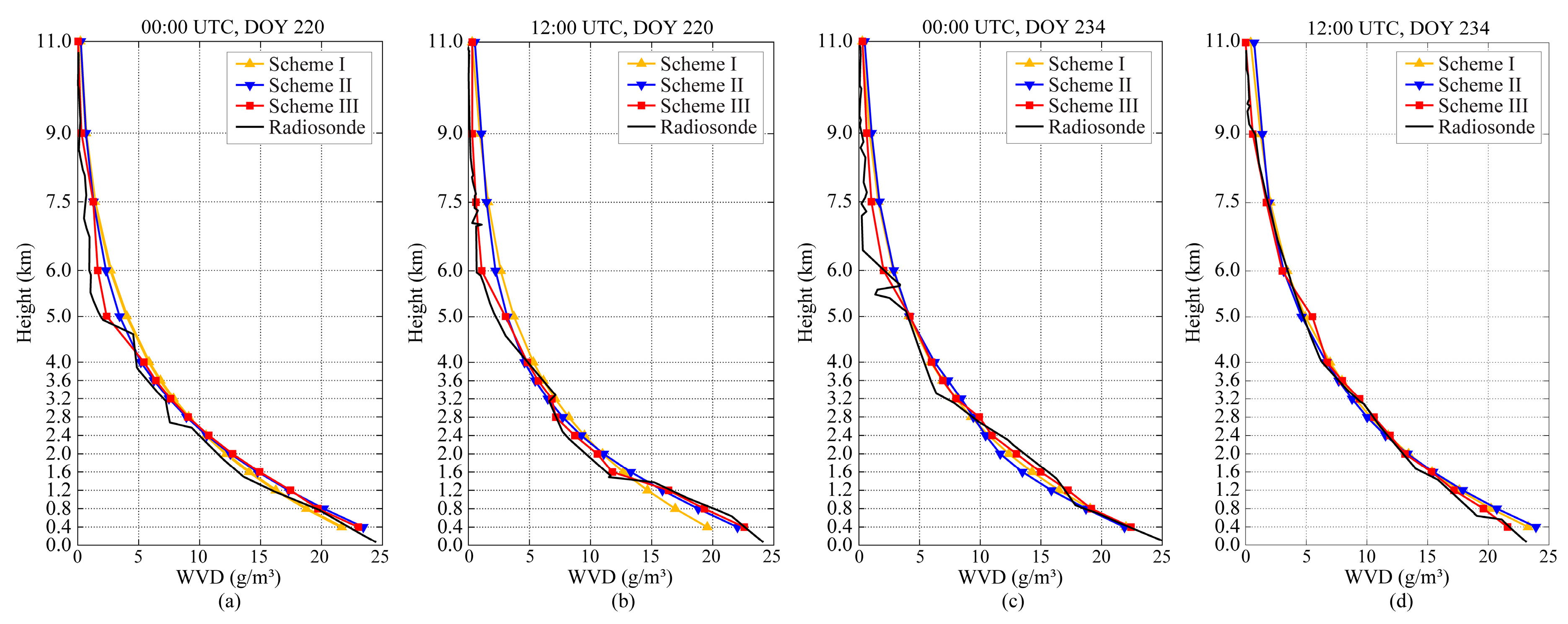
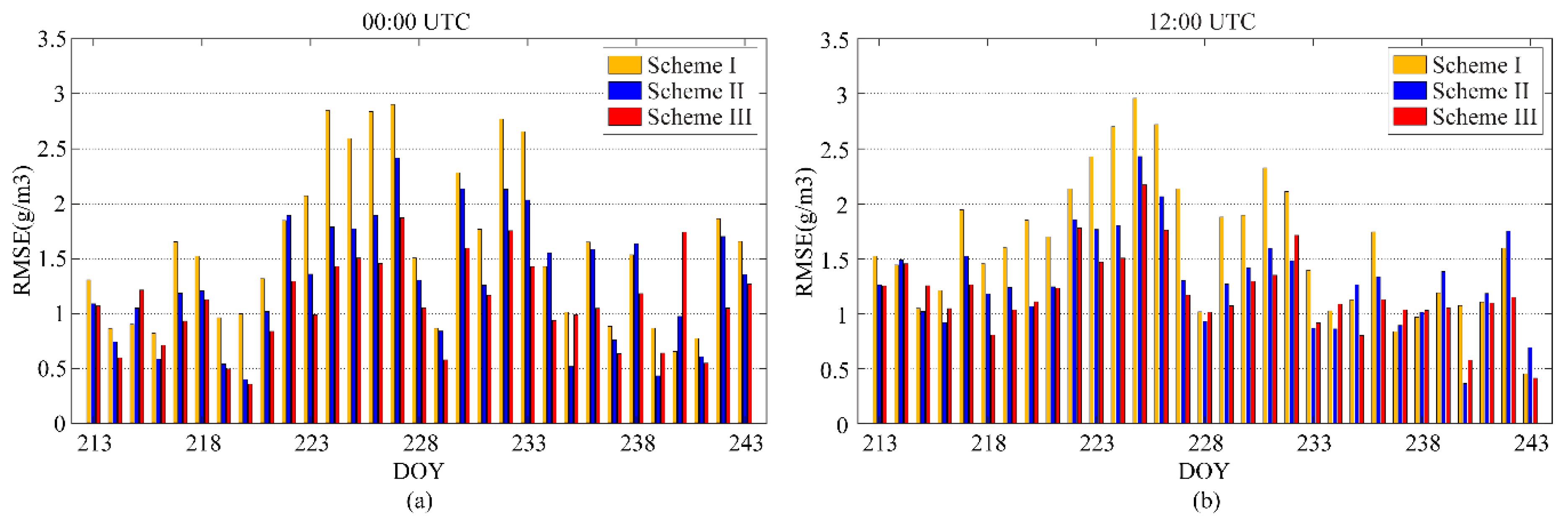
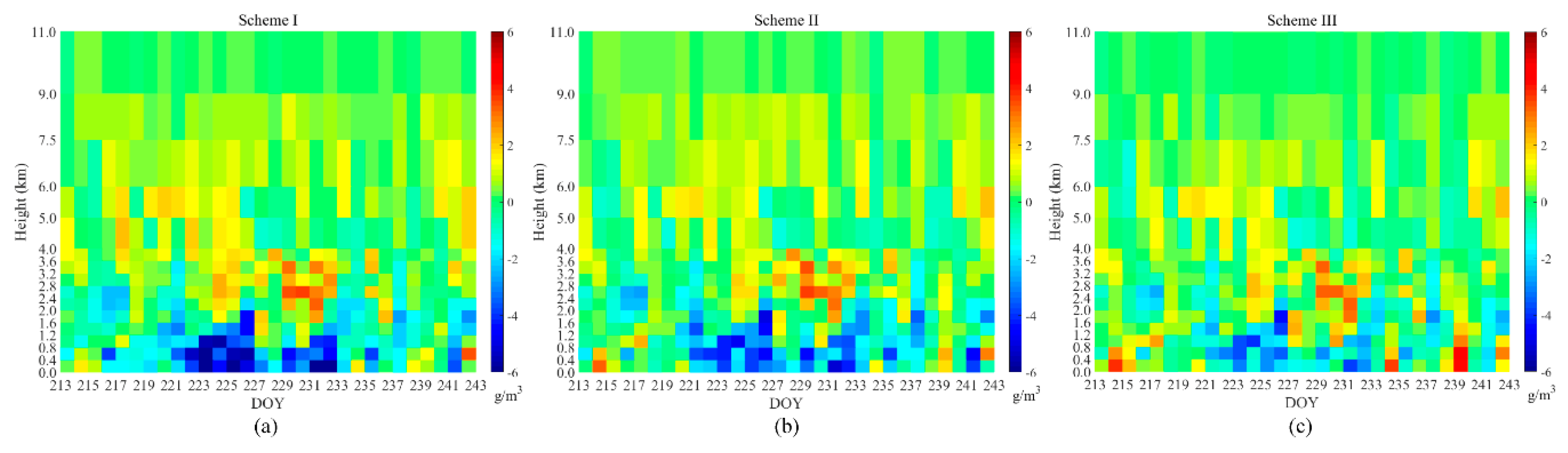
• Scheme I: The traditional tomography method that only considers the GNSS signals crossing the top boundary is adopted to construct the observation equations;
• Scheme II: The Yao model is used to estimate the SWV of side rays and build the equations with both rays passing from the top and side boundary;
• Scheme III: The HFM is employed to calculate the $SW{V}_{side}$ and structure the tomography system with top and side observations.

Based on GNSS data at two tomography epochs of 00:00-00:30 UTC and 12:00-12:30 UTC during the period of DOY 213-243, 2017, the scale factor in the Yao model was calculated and is illustrated in Figure 13, where a similar exponential relationship can be observed. It is noticeable that owing to the neglection of GNSS signals with an elevation angle of less than 15°, all of the heights of the intersection points are higher than approximately 1 km. Accordingly, the coefficients $a$ and $b$ were estimated by the least-squares method, and the results are given in

Table 5. The fitting coefficient and accuracy of the Yao model.

Model	$\mathit{a}$	$\mathit{b}$	RMSE	R-Square
Yao model	2.233	−1.119	0.9882	0.0145

[27].

With the scale factor in the Yao model and the HFM proposed in this paper, the SWV of the side signals could be estimated based on the height of the intersection points. Consequently, Figure 14 presents a comparison of the SWV value of effective side rays between the Yao model and HFM at two tomography epochs during each of the test days. It is clear that the HFM can estimate slightly higher SWV values than the Yao model for most signals, and the latter provides a rather small SWV estimation, with a value of approximately 20 mm, for several observation rays.

To assess the water vapor reconstruction capabilities of different methods, the tomographic results derived from the three schemes, described in Figure 15, were employed to illustrate the water vapor vertical profile at 00:00 UTC and 12:00 UTC on DOY 220 (sunny day) and DOY 234 (rainy day).

It can be observed that the water vapor profiles derived from the three considered schemes agree with the reference profile obtained by the radiosonde data. Furthermore, a higher coincidence of the vertical profile can be seen on majority layers when combining the inside signals. As far as the quantitative comparison of WVD is concerned, the accuracy of the tomographic solutions from Scheme III (mean RMSE are 0.69 and 0.95 g/m³ on both days) is superior to those from Scheme I (mean RMSE are 1.40 and 1.30 g/m³ on both days) and Scheme II (mean RMSE are 0.73 and 1.20 g/m³ on both days), which reveals that the proposed model has better reconstruction capabilities than the Yao model and traditional model in both weather conditions.

In addition, to further show the superiority of the proposed method in the WVD comparison, the RMSE of tomographic results from the three schemes was calculated, and the results are shown in Figure 16, including the 31-day period from DOY 213 to DOY 243, 2017, at 00:00 and 12:00 UTC daily. It is clear that, among the three schemes, Scheme III has the smallest RMSE compared to Scheme I and Scheme II in the majority of time periods. The average improvement of Scheme III with respect to Scheme I and Scheme II was 0.51 and 0.20 g/m³ in terms of the RMSE, respectively. As a further assessment, Table 2 lists the statistics of the three tomography solutions, including the maximum, minimum, and mean values of RMSE, STD, and bias.

It should be noted from

Table 6. Statistics (RMSE, STD, and bias) of the tomography results for the three schemes (unit: g/m³).

Scheme	RMSE			STD			Bias
	Max.	Min.	Mean	Max.	Min.	Mean	Max.	Min.	Mean
Scheme I	3.36	0.50	1.59	3.37	0.45	1.60	0.55	−1.26	−0.26
Scheme II	2.42	0.40	1.28	2.30	0.41	1.25	0.66	−1.33	−0.14
Scheme III	1.98	0.28	1.08	2.00	0.29	1.07	0.87	−0.55	0.16

that all of the means of the three statistics in Scheme II and III are superior to those of Scheme I, which suggests that there is an improvement of the GNSS tomography solution when side observations are included in the tomography modeling. As far as Scheme II and III are concerned, the average RMSE and STD for the former are 1.28 and 1.25 g/m³ and the latter are 1.08 and 1.07 g/m³, respectiely, and the mean accuracy improvement rates are 15.62% and 14.40% for both statistics, respectively, which demonstrates that the proposed HFM provides more accurate side SWV observations and three-dimensional water vapor fields.

Following this, to quantitatively compare the accuracy of each layer’s tomographic results, the reference value of WVD, along the vertical columns, was interpolated using the radiosonde data, and the mean difference between the tomographic results obtained from the three schemes and the radiosonde data during the tomographic period was calculated and is reported in Figure 17. It is evident that the absolute value of the average differences dramatically decreases with increasing height layers. Besides, it should be noted that in the earth surface layer from 0 to 2 km, the difference of most voxels is less than 0 in the three schemes, i.e., the WVD retrieved from the GNSS tomography solution is lower than that obtained from the radiosonde. However, it is noticeable that there is an impressive improvement of the WVD in these layers in Scheme II and Scheme III, although the voxels in this range are not penetrated by side signals according to Figure 10. This can be explained by the fact that when combining both integral signals and inside ones for GNSS tomography, the number of effective observations is obviously increased and the spatial geometric defect of the three-dimensional tomographic model and the ill condition of the tomographic observation equations are gradually remedied, which is beneficial for improving the accuracy and stability of the tomography results.

Furthermore, the conclusion that the differences of Scheme III are smaller than those of Scheme II in each layer can be drawn from Figure 17, which highlights the advantages of the proposed HFM. This could be because of the higher side SWV observations estimated from the HFM in Figure 14, which results in the tomography solutions being closer to the radiosonde measurements.

5. Conclusions

A novel tropospheric tomography methodology based on the HFM, combining integral and side signals, has been introduced and demonstrated in this paper. The SWD of GNSS rays, which is a crucial observation for the GNSS tomography system, has been separated into two parts—isotropic and anisotropic components—corresponding to the isotropic and anisotropic height factors in the HFM. With these two factors, the SWD of the side rays can be estimated accurately. It should be noted that the signals with an elevation angle of less than 15° were eliminated due to bending of the ray path. In addition, the dynamic tomography top boundary was determined based on 30-year radiosonde data, which preserved highly accurate water vapor profiles at different altitudes.

The proposed method was validated and assessed by four special schemes, in which the tomography area was adjusted to force the RS-voxels located in different tomographic boundaries. When the input of the tomography system was only integral signals, the average utilization of GNSS signals was 47.12%, and the mean RMSE and STD were 1.63 and 1.61 g/m³, respectively. When side rays were combined, the former was increased to 80.54% and was stable for the four schemes. The latter was improved to 1.16 and 1.15 g/m³, respectively. In the four experimental comparisons, whether in terms of RMSE or STD, it was observed that there was a significant improvement of the tomography results with the side signals. Furthermore, a special comparison of the proposed method and one existing correction approach was performed based on the three other schemes. Compared to the currently optimized model, the tomography results of the proposed model showed mean accuracy improvement rates of 15.62% and 14.40% in terms of the RMSE and STD, separately, which highlights the advantages of the proposed HFM in estimating the side SWV observations and retrieving the three-dimensional water vapor field.

In addition, the proposed HFM method provides a new way to address the tropospheric delays. From the perspective of isotropic and anisotropic components, some issues resulting from atmospheric water vapor may be skillfully handled, e.g., tropospheric delay correction in InSAR and VLBI, which may inspire new concepts for relevant researchers. Future work will focus on assimilating multi-source remote sensing data into tropospheric tomography, e.g., MODIS, MERIS, and InSAR, providing high-resolution PWV maps, which may be useful for GNSS tomography.

References

1. Benevides, P.; Catalao, J.; Miranda, P.M.A. On the inclusion of GPS precipitable water vapour in the nowcasting of rainfall. Nat. Hazard Earth Syst. 2015, 15, 2605–2616. [Google Scholar] [CrossRef] [Green Version]
2. Chen, B.Y.; Liu, Z.Z.; Wong, W.K.; Woo, W.C. Detecting Water Vapor Variability during Heavy Precipitation Events in Hong Kong Using the GPS Tomographic Technique. J. Atmos. Ocean. Technol. 2017, 34, 1001–1019. [Google Scholar] [CrossRef]
3. Guerova, G.; Jones, J.; Dousa, J.; Dick, G.; Haan, S.; Pottiaux, E.; Bock, O.; Pacione, R.; Elgered, G.; Vedel, H.; et al. Review of the State-of-the-Art and Future Prospects of the Ground-Based GNSS Meteorology in Europe. Atmos. Meas. Tech. 2016, 9, 5385–5406. [Google Scholar] [CrossRef] [Green Version]
4. Zhao, Q.; Liu, Y.; Ma, X.; Yao, W.; Yao, Y.; Li, X. An Improved Rainfall Forecasting Model Based on GNSS Observations. IEEE Trans. Geosci. Remote Sens. 2020, 1–10. [Google Scholar] [CrossRef]
5. Lu, C.; Li, X.; Ge, M.; Heinkelmann, R.; Nilsson, T.; Soja, B.; Dick, G.; Schuh, H. Estimation and evaluation of real-time precipitable water vapor from GLONASS and GPS. GPS Solut. 2016, 20, 703–713. [Google Scholar] [CrossRef] [Green Version]
6. Wang, X.; Zhang, K.; Wu, S.; Li, Z.; Cheng, Y.; Li, L.; Yuan, H. The correlation between GNSS-derived precipitable water vapor and sea surface temperature and its responses to El Niño–Southern Oscillation. Remote Sens. Environ. 2018, 216, 1–12. [Google Scholar] [CrossRef]
7. Flores, A.; Ruffini, G.; Rius, A. 4D tropospheric tomography using GPS slant wet delays. In Annales Geophysicae; Springer: Berlin, Germany, 2000. [Google Scholar]
8. Gradinarsky, L.; Jarlemark, P. Ground-Based GPS Tomography of Water Vapor: Analysis of Simulated and Real Data. J. Meteorol. Soc. Jpn. 2004, 82, 551–560. [Google Scholar] [CrossRef] [Green Version]
9. Champollion, C.; Masson, F.; Bouin, M.; Walpersdorf, A.; Doerflinger, E.; Bock, O.; Van Baelen, J. GPS water vapour tomography: Preliminary results from the ESCOMPTE field experiment. Atmos. Res. 2005, 74, 253–274. [Google Scholar] [CrossRef] [Green Version]
10. Bender, M.; Dick, G.; Ge, M.; Deng, Z.; Wickert, J.; Kahle, H.-G.; Raabe, A.; Tetzlaff, G. Development of a GNSS water vapour tomography system using algebraic reconstruction techniques. Adv. Space Res. 2010, 47, 1704–1720. [Google Scholar] [CrossRef] [Green Version]
11. Rohm, W.; Bosy, J. The verification of GNSS tropospheric tomography model in a mountainous area. Adv. Space Res. 2011, 47, 1721–1730. [Google Scholar] [CrossRef]
12. Benevides, P.; Catalão, J.; Miranda, P. Estudio experimental de tomografía GNSS en Lisboa (Portugal). Física De La Tierra 2014, 26. [Google Scholar] [CrossRef] [Green Version]
13. Heublein, M.; Zhu, X.X.; Alshawaf, F.; Mayer, M.; Bamler, R.; Hinz, S. Compressive sensing for neutrospheric water vapor tomography using GNSS and InSAR observations. In Proceedings of the International Geoscience and Remote Sensing Symposium, Milan, Italy, 26–31 July 2015; pp. 5268–5271. [Google Scholar]
14. Yao, Y.; Zhao, Q. Maximally Using GPS Observation for Water Vapor Tomography. IEEE Trans. Geosci. Remote Sens. 2016, 54, 7185–7196. [Google Scholar] [CrossRef]
15. Benevides, P.; Nico, G.; Catalao, J.; Miranda, P.M.A. Bridging InSAR and GPS Tomography: A New Differential Geometrical Constraint. IEEE Trans. Geosci. Remote Sens. 2016, 54, 697–702. [Google Scholar] [CrossRef]
16. Benevides, P.; Catalao, J.; Nico, G.; Miranda, P.M.A. 4D wet refractivity estimation in the atmosphere using GNSS tomography initialized by radiosonde and AIRS measurements: Results from a 1-week intensive campaign. GPS Solut. 2018, 22, 91. [Google Scholar] [CrossRef]
17. Trzcina, E.; Rohm, W. Estimation of 3D wet refractivity by tomography, combining GNSS and NWP data: First results from assimilation of wet refractivity into NWP. Q. J. R. Meteorol. Soc. 2019, 145, 1034–1051. [Google Scholar] [CrossRef]
18. Zhang, W.; Zhang, S.; Nan, D.; Pengxu, M. An improved tropospheric tomography method based on the dynamic node parametrized algorithm. Acta Geodyn. Geomater. 2020, 191–206. [Google Scholar] [CrossRef]
19. Rohm, W. The ground GNSS tomography–unconstrained approach. Adv. Space Res. 2013, 51, 501–513. [Google Scholar] [CrossRef]
20. Zhao, Q.; Yao, Y.; Yao, W. Troposphere Water Vapour Tomography: A Horizontal Parameterised Approach. Remote Sens. 2018, 10, 1241. [Google Scholar] [CrossRef] [Green Version]
21. Song, S.; Zhu, W.; Ding, J.; Peng, J. 3D water-vapor tomography with Shanghai GPS network to improve forecasted moisture field. Chin. Sci. Bull. 2006, 51, 607–614. [Google Scholar] [CrossRef]
22. Xia, P.; Cai, C.; Liu, Z. GNSS troposphere tomography based on two-step reconstructions using GPS observations and COSMIC profiles. Ann. Geophys. 2013, 31, 1805–1815. [Google Scholar] [CrossRef] [Green Version]
23. Benevides, P.; Nico, G.; Catalao, J.; Miranda, P.M.A. Analysis of Galileo and GPS Integration for GNSS Tomography. IEEE Trans. Geosci. Remote Sens. 2017, 55, 1936–1943. [Google Scholar] [CrossRef]
24. Dong, Z.; Jin, S. 3-D Water Vapor Tomography in Wuhan from GPS, BDS and GLONASS Observations. Remote Sens. 2018, 10, 62. [Google Scholar] [CrossRef] [Green Version]
25. Zhao, Q.; Yao, Y.; Cao, X.; Zhou, F.; Xia, P. An Optimal Tropospheric Tomography Method Based on the Multi-GNSS Observations. Remote Sens. 2018, 10, 234. [Google Scholar] [CrossRef] [Green Version]
26. Heublein, M.; Alshawaf, F.; Erdnüß, B.; Zhu, X.X.; Hinz, S. Compressive sensing reconstruction of 3D wet refractivity based on GNSS and InSAR observations. J. Geod. 2019, 93, 197–217. [Google Scholar] [CrossRef] [Green Version]
27. Zhao, Q.; Zhang, K.; Yao, Y.; Li, X. A new troposphere tomography algorithm with a truncation factor model (TFM) for GNSS networks. GPS Solut. 2019, 23, 64. [Google Scholar] [CrossRef]
28. Landskron, D.; Böhm, J. Refined discrete and empirical horizontal gradients in VLBI analysis. J. Geod. 2018, 92, 1387–1399. [Google Scholar] [CrossRef] [PubMed] [Green Version]
29. Yu, C.; Li, Z.; Penna, N.T.; Crippa, P. Generic Atmospheric Correction Model for Interferometric Synthetic Aperture Radar Observations. J. Geophys. Res. Solid Earth 2018, 123, 9202–9222. [Google Scholar] [CrossRef]
30. Bevis, M.; Businger, S.; Herring, T.A.; Rocken, C.; Anthes, R.A.; Ware, R.H. GPS meteorology remote sensing of atmospheric water vapor using global positioning system. J. Geophys. Res. Atmos. 1992, 97, 15787–15801. [Google Scholar] [CrossRef]
31. Gardner, S.C. Effects of horizontal refractivity gradients on the accuracy of laser ranging to satellites. Radio Sci. 1977, 11, 1037–1044. [Google Scholar] [CrossRef]
32. Boehm, J.; Schuh, H. Troposphere gradients from the ECMWF in VLBI analysis. J. Geod. 2007, 81, 403–408. [Google Scholar] [CrossRef]
33. Chen, G.; Herring, T.A. Effects of atmospheric azimuthal asymmetry on the analysis of space geodetic data. J. Geophys. Res. Atmos. 1997, 102, 20489. [Google Scholar] [CrossRef]
34. Alber, C.; Ware, R.; Rocken, C.; Braun, J. Obtaining single path phase delays from GPS double differences. Geophys. Res. Lett. 2000, 27, 2661–2664. [Google Scholar] [CrossRef] [Green Version]
35. Davis, J.L.; Herring, T.A.; Shapiro, I.I.; Rogers, A.E.E.; Elgered, G. Geodesy by Radio Interferometry: Effects of Atmospheric Modeling Errors on Estimates of Baseline Length. Radio Sci. 1985, 20, 1593–1607. [Google Scholar] [CrossRef]
36. Chen, B.Y.; Liu, Z.Z. Voxel-optimized regional water vapor tomography and comparison with radiosonde and numerical weather model. J. Geod. 2014, 88, 691–703. [Google Scholar] [CrossRef]
37. Perler, D.; Geiger, A.; Hurter, F. 4D GPS water vapor tomography: New parameterized approaches. J. Geod. 2011, 85, 539–550. [Google Scholar] [CrossRef] [Green Version]
38. Chen, B.; Liu, Z. Global water vapor variability and trend from the latest 36 year (1979 to 2014) data of ECMWF and NCEP reanalyses, radiosonde, GPS, and microwave satellite. J. Geophys. Res. Atmos. 2016, 121, 442–411, 462. [Google Scholar] [CrossRef]
39. Zhao, Q.; Yao, W.; Yao, Y.; Li, X. An improved GNSS tropospheric tomography method with the GPT2w model. GPS Solut. 2020, 24, 60. [Google Scholar] [CrossRef]
40. Nilsson, T.; Böhm, J.; Wijaya, D.D.; Tresch, A.; Schuh, H. Path Delays in the Neutral Atmosphere; Springer: Berlin, Germany, 2013. [Google Scholar]
41. Ding, N.; Zhang, S.B.; Wu, S.Q.; Wang, X.M.; Zhang, K.F. Adaptive Node Parameterization for Dynamic Determination of Boundaries and Nodes of GNSS Tomographic Models. J. Geophys. Res. Atmos. 2018, 123, 1990–2003. [Google Scholar] [CrossRef]
42. Möller, G.; Landskron, D. Atmospheric bending effects in GNSS tomography. Atmos. Meas. Tech. 2019, 12, 23–34. [Google Scholar] [CrossRef] [Green Version]
43. Xia, P.; Ye, S.; Jiang, P.; Pan, L.; Guo, M. Assessing water vapor tomography in Hong Kong with improved vertical and horizontal constraints. In Annales Geophysicae; Copernicus GmbH: Göttingen, Germnay, 2018; pp. 1–28. [Google Scholar] [CrossRef] [Green Version]
44. Xiaoying, W.; Ziqiang, D.; Enhong, Z.; Fuyang, K.E.; Yunchang, C.; Lianchun, S. Tropospheric wet refractivity tomography using multiplicative algebraic reconstruction technique. Adv. Space Res. 2013, 53, 156–162. [Google Scholar] [CrossRef]
45. Saastamoinen, J. Contributions to the theory of atmospheric refraction. J. Geod. 1972, 105, 279–298. [Google Scholar] [CrossRef]
46. Boehm, J.; Schuh, H. Vienna mapping functions in VLBI analyses. Geophys. Res. Lett. 2004, 31, 277. [Google Scholar] [CrossRef]
47. Ding, N.; Zhang, S.; Wu, S.; Wang, X.; Kealy, A.; Zhang, K. A new approach for GNSS tomography from a few GNSS stations. Atmos. Meas. Tech. 2018, 11, 3511–3522. [Google Scholar] [CrossRef] [Green Version]
Figure 1. The distribution of water vapor derived from 30 years of radiosonde data in the atmosphere for different months. (a) The vertical distribution of atmospheric water vapor. The black ellipse in (a) represents the outliers; (b) enlarged view corresponding to the blue rectangle in (a). Blue vertical lines in (b) correspond to the principle that the water vapor density (WVD) is 0.2 g/m3, and the blue horizontal lines denote the optimal top boundary during different months.
Remotesensing 12 01848 g001
Figure 2. Two-dimensional schematic diagram of the height factor model (HFM) to illustrate the estimation method of sectional slant wet delay (SWD) for top and side signals.
Remotesensing 12 01848 g002
Figure 3. The isotropic height factor changes with height in different months. (a) January; (b) February; (c) March; (d) April; (e) May; (f) June; (g) July; (h) August; (i) September; (j) October; (k) November; and (l) December.
Remotesensing 12 01848 g003
Figure 4. The (a) root mean square error (RMSE) and (b) R-square of the least-squares fitting results of different months.
Remotesensing 12 01848 g004
Figure 5. The anisotropic height factor changes with height.
Remotesensing 12 01848 g005
Figure 6. A comparison of the flow chart of the traditional tomography model (a) and the improved model (b).
Remotesensing 12 01848 g006
Figure 7. (a) Plane map of the Hong Kong area obtained by Mercator projection with 17 Global Navigation Satellite System (GNSS) reference stations (red dots) and radiosonde King’s Park Meteorological Station (HKKP) (blue dot) in Hong Kong; (b) 3-D distribution of GPS signals for the proposed tomography model. Red lines represent signals passing from the top boundary of the tomographic area, whereas green lines denote rays penetrating from the side face of the tomography region. The blue vertical columns represent the radiosonde (RS)-voxels where the radiosonde is located.
Remotesensing 12 01848 g007
Figure 8. The tomographic region (red rectangles) for four schemes. (a) Scheme East; (b) Scheme West; (c) Scheme South; and (d) Scheme North. The blue square refers to the RS-voxels.
Remotesensing 12 01848 g008
Figure 9. The slant water vapor (SWV) value of inside signals in four schemes: top for total SWV, center for isotropic SWV, and bottom for anisotropic SWV, respectively. (a) Scheme East; (b) Scheme West; (c) Scheme South; and (d) Scheme North.
Remotesensing 12 01848 g009
Figure 10. The number of penetrated signals in the RS-voxels column, where the abscissa represents the bottom-up column voxel numbering. (a) Scheme East; (b) Scheme West; (c) Scheme South; and (d) Scheme North.
Remotesensing 12 01848 g010
Figure 11. The average number of effective signals (a) and the mean utilization rate of signals (b) for the two methods during the period of DOY 213-243, 2017.
Remotesensing 12 01848 g011
Figure 12. Comparison of the SWV differences between the observed SWV and retrieved SWV from the three-dimensional tomographic water vapor field with the two methods in the four schemes. (a) Scheme East; (b) Scheme West; (c) Scheme South; and (d) Scheme North.
Remotesensing 12 01848 g012
Figure 13. The scale factor changes with the height of the intersection point between the effective side signals and the side face of the tomographic area during the period of DOY 213-243, 2017.
Remotesensing 12 01848 g013
Figure 14. Comparison of the SWV value of effective side rays obtained from the Yao model and the HFM for two tomography epochs. (a) 00:00–00:30 UTC; (b) 12:00–12:30 UTC.
Remotesensing 12 01848 g014
Figure 15. Comparison of the tomographic water vapor profiles for three schemes under different weather conditions using the radiosonde data (black lines) as a reference. (a) 00:00 UTC, DOY 220; (b) 12:00 UTC, DOY 220; (c) 00:00 UTC, DOY 234; and (d) 12:00 UTC, DOY 234.
Remotesensing 12 01848 g015
Figure 16. Comparisons of the RMSE of the tomography results derived from different schemes during the 31-day period from DOY 213 to DOY 243, 2017, at (a) 00:00 UTC and (b) 12:00 UTC daily.
Remotesensing 12 01848 g016
Figure 17. The mean differences between the tomographic results and radiosonde data along the radiosonde vertical columns from DOY 213 to DOY 243, 2017. (a) Scheme I; (b) Scheme II; and (c) Scheme III.
Remotesensing 12 01848 g017