Unsupervised Satellite Image Time Series Clustering Using Object-Based Approaches and 3D Convolutional Autoencoder


Abstract
1. Introduction
- We propose a fully unsupervised approach of SITS clustering using deep learning approaches.
- We propose a two-branch multi-view AE that extracts more robust features comparatively to a classic convolutional AE.
- We develop a segmentation approach that produces a unique segmentation map for the whole SITS.
- The proposed architecture is new and does not rely on a pre-existing or pre-trained network.
2. Methodology
- We start by relative normalization of all the images of the SITS using an algorithm described in Reference [29] and correction of saturated pixels.
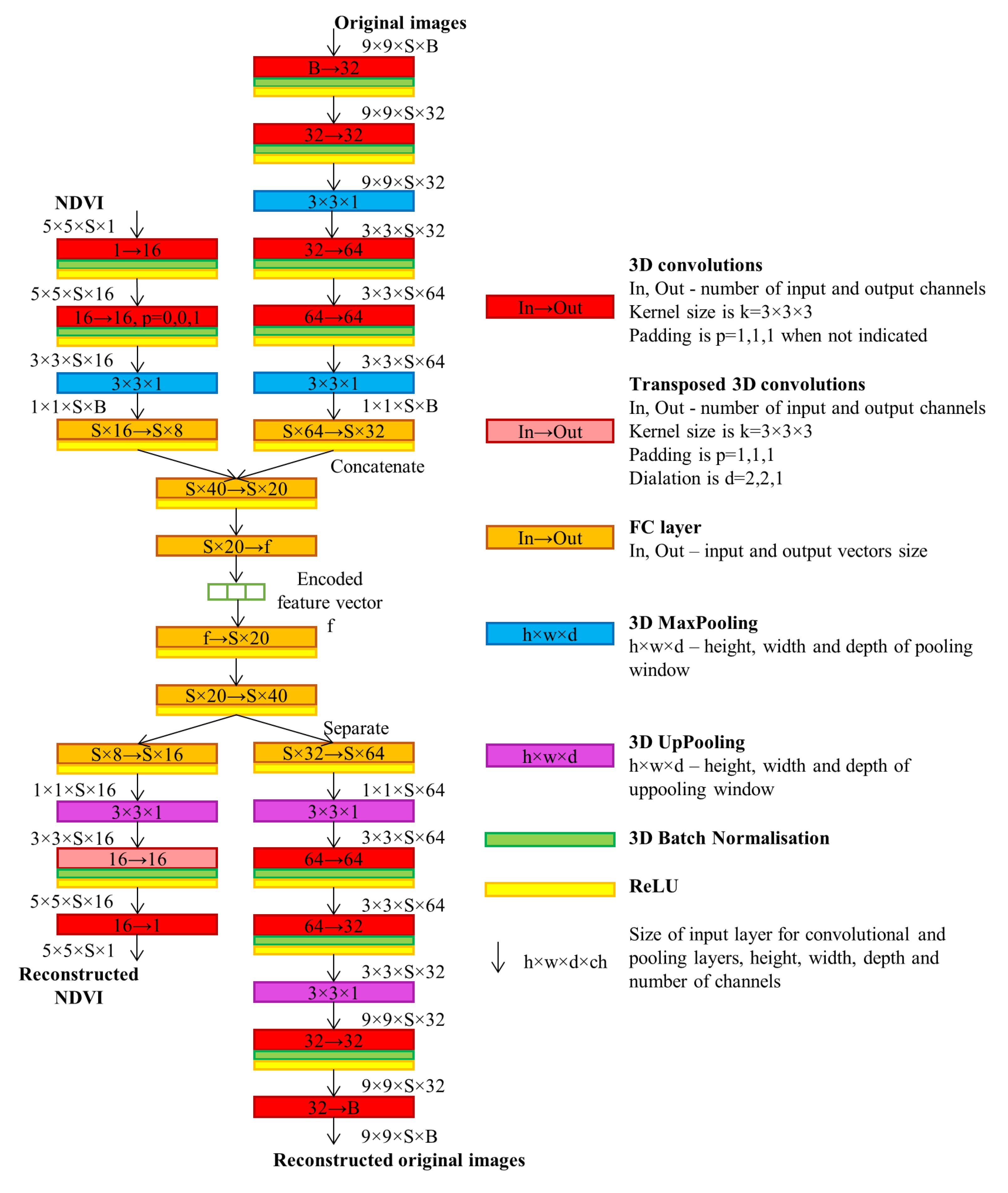
- We deploy a two-branch multi-view 3D convolutional AE model in order to extract spatio-temporal features and compress the SITS.
- Then, we perform a preliminary SITS segmentation using two farthest images of the dataset taken in different seasons.
- We correct the preliminary change segmentation using the compressed SITS.
- Finally, we perform the clustering of extracted segments using their spatio-temporal features as descriptors.
2.1. Time Series Encoding
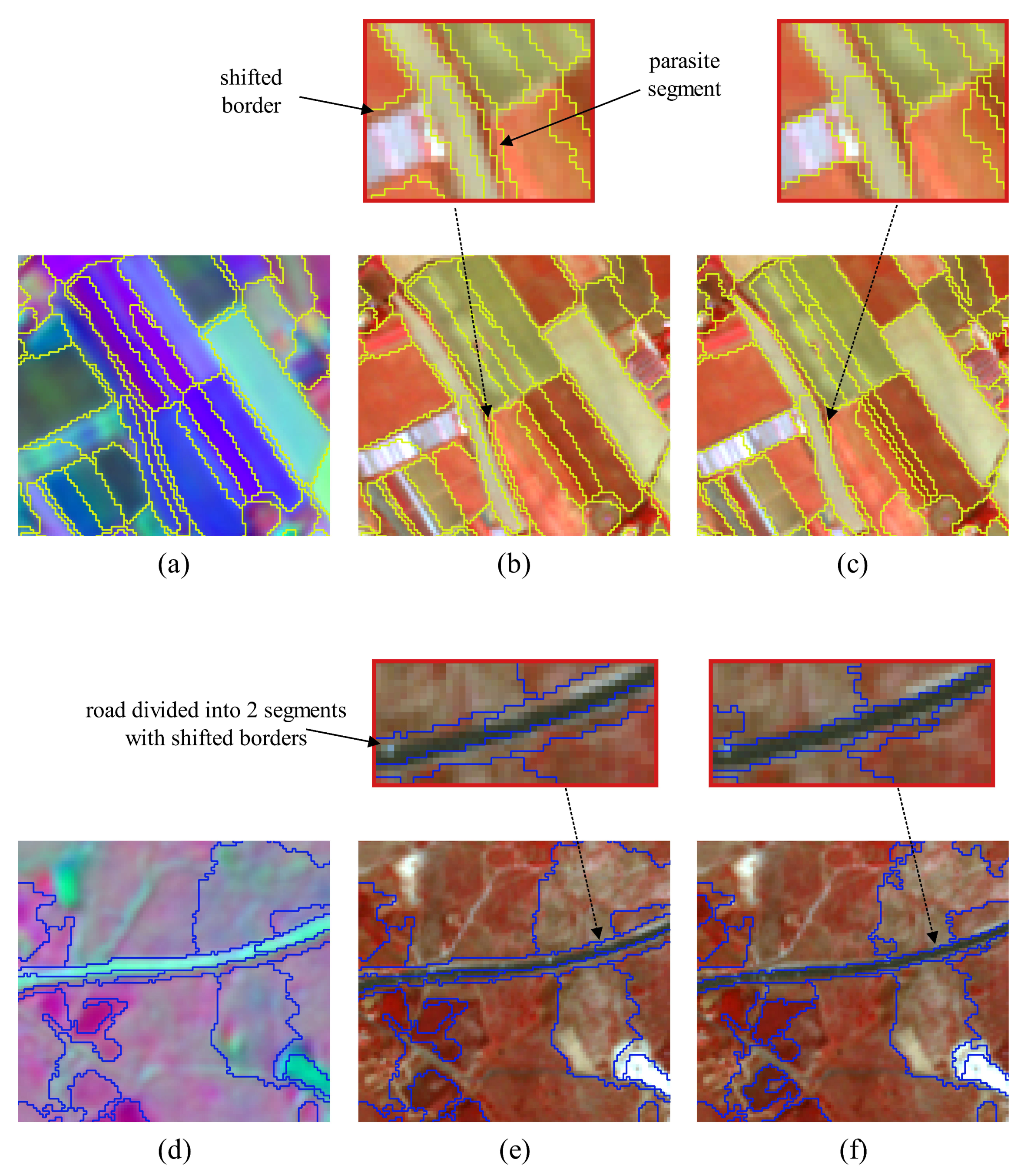
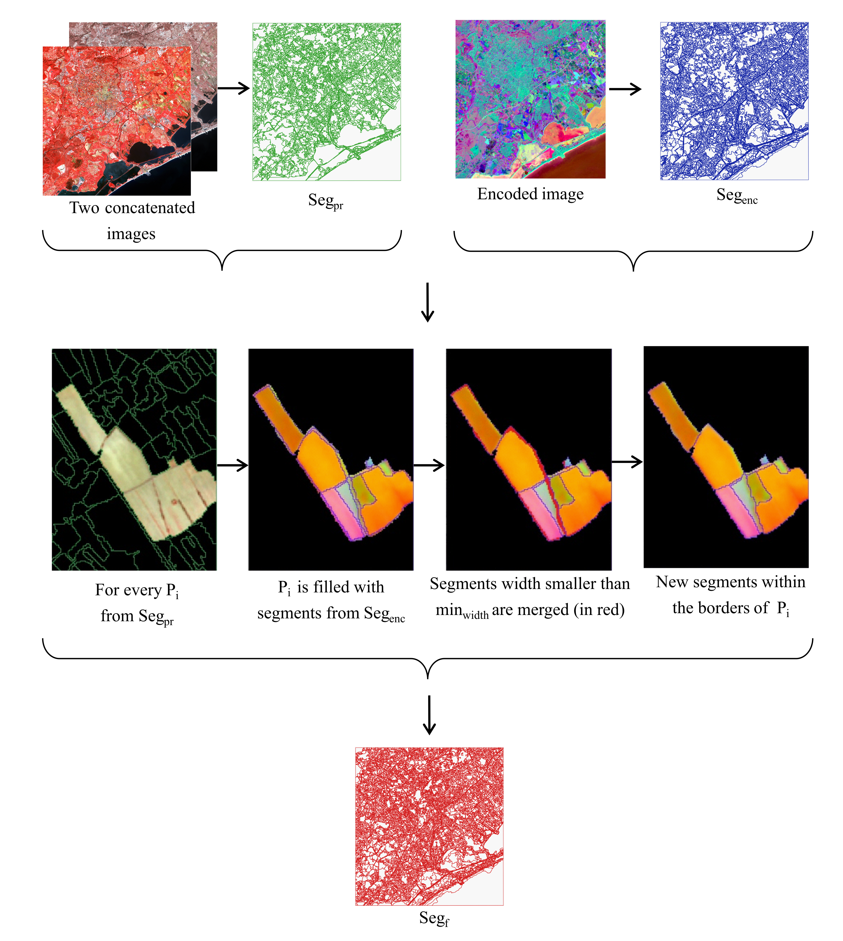
2.2. Segmentation
- Let be a segment from to correct.
- We firstly fill with the segments from that have spatial intersection with it. borders are preserved and used as the reference.
- Second, we check the average width of these segments in horizontal and vertical axes of the SITS coordinate system. We select objects with width smaller than in at least one of the axes. size should not exceed half of the encoder patch size and be set after estimating the influence of the border effect.
- At the third place, each of these objects is merged with a neighbor with the biggest common edge if the edge is at least 3 pixels long or if the object’s size does not exceed (minimum object size that we want to distinguish in our experiments). Note that in case we have several segments to merge, we sort them by ascending size and start by merging the smallest one while other segments sizes are being iteratively updated.
- Finally, we fill a new segmentation map with new merged segments.
2.3. Clustering
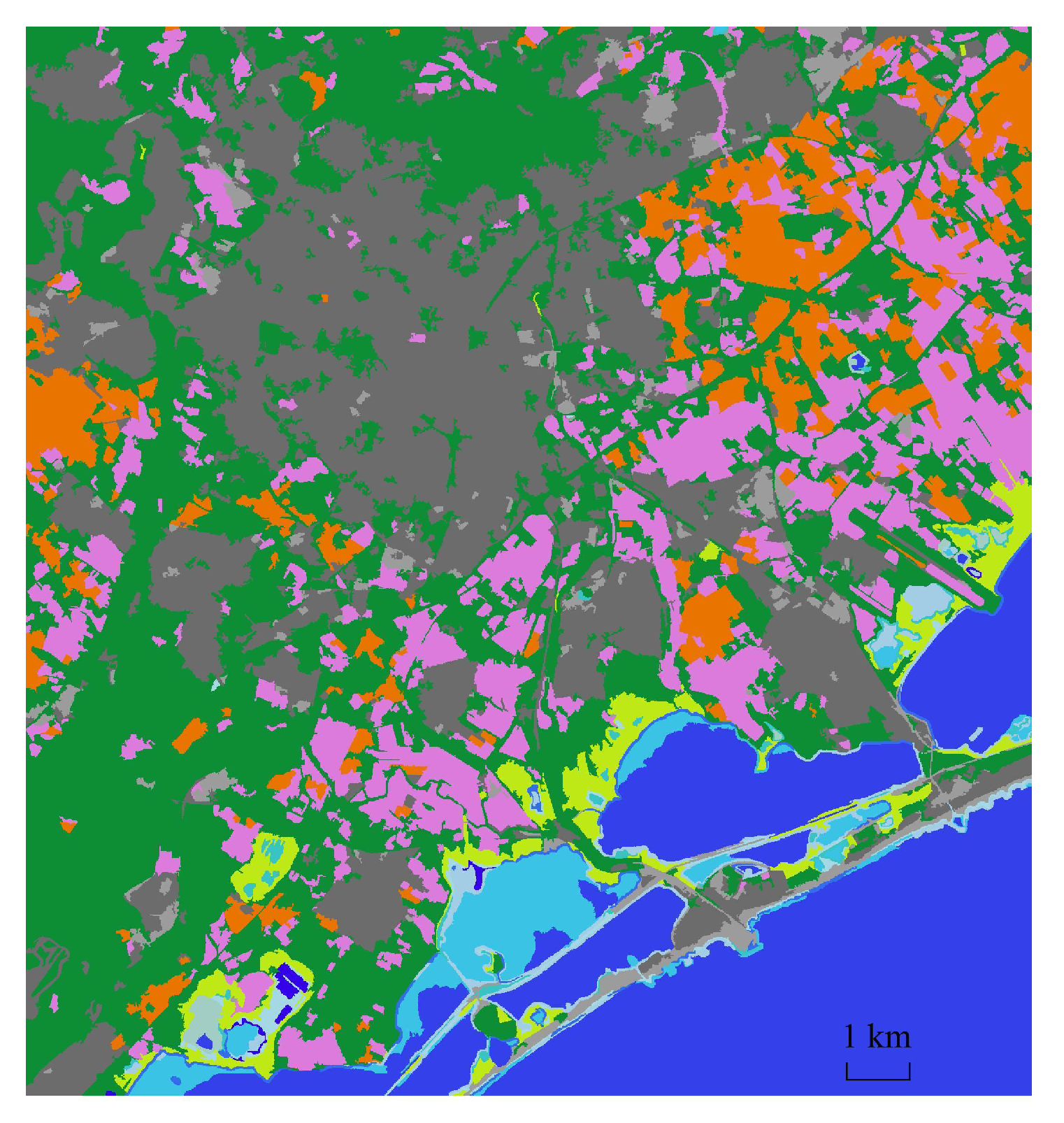
3. Data
- bottom left corner: 43°30′6.0444″N, 3°47′30.066″E
- top right corner: 43°39′22.4856″N, 3°59′31.596″E
- urban and artificial area,
- wooded area (include forests, parks, family gardens etc.),
- natural area (not wooded),
- water surface,
- annual crops,
- prairies,
- vineyards,
- orchards,
- olive plantation.
4. Experiments
4.1. Experimental Settings
4.1.1. Time Series Encoding
4.1.2. Preliminary Segmentation
4.1.3. Correction of Segmentation Results
4.1.4. Clustering
4.2. Results
- Object-based (OB) DTW—as the segmentation reference we use the preliminary segmentation results for our method, we exploit hierarchical clustering algorithm with DTW distance matrix to regroup the obtained segments.
- Graph-based (GB) DTW—we use MeanShift algorithm with the following parameters to segment every image of the SITS , , for SPOT-5 dataset and , , for Sentinel-2 dataset. For both datasets we use the following parameters for graph construction, see Reference [18] for details: , . We omit as it lowers the quality of the results. The hierarchical clustering method with DTW distance matrix is applied as in the original article.
- 3D convolutional AE without NDVI branch—we use the same pipeline and segmentation parameters as in our proposed method, however, the feature extraction model is different. For feature maps extraction, we have the same 4 convolutional and 2 maxpooling layers as in the original images branch that are followed by 2 FC layers with the following input and output sizes for the encoding part: , . The decoder FC layers are symmetrical to the encoder.
- 3D convolutional AE without segmentation correction—we use the same pipeline and segmentation parameters as in our proposed method, however, the clustering is performed for the preliminary segmentation made for two concatenated images.
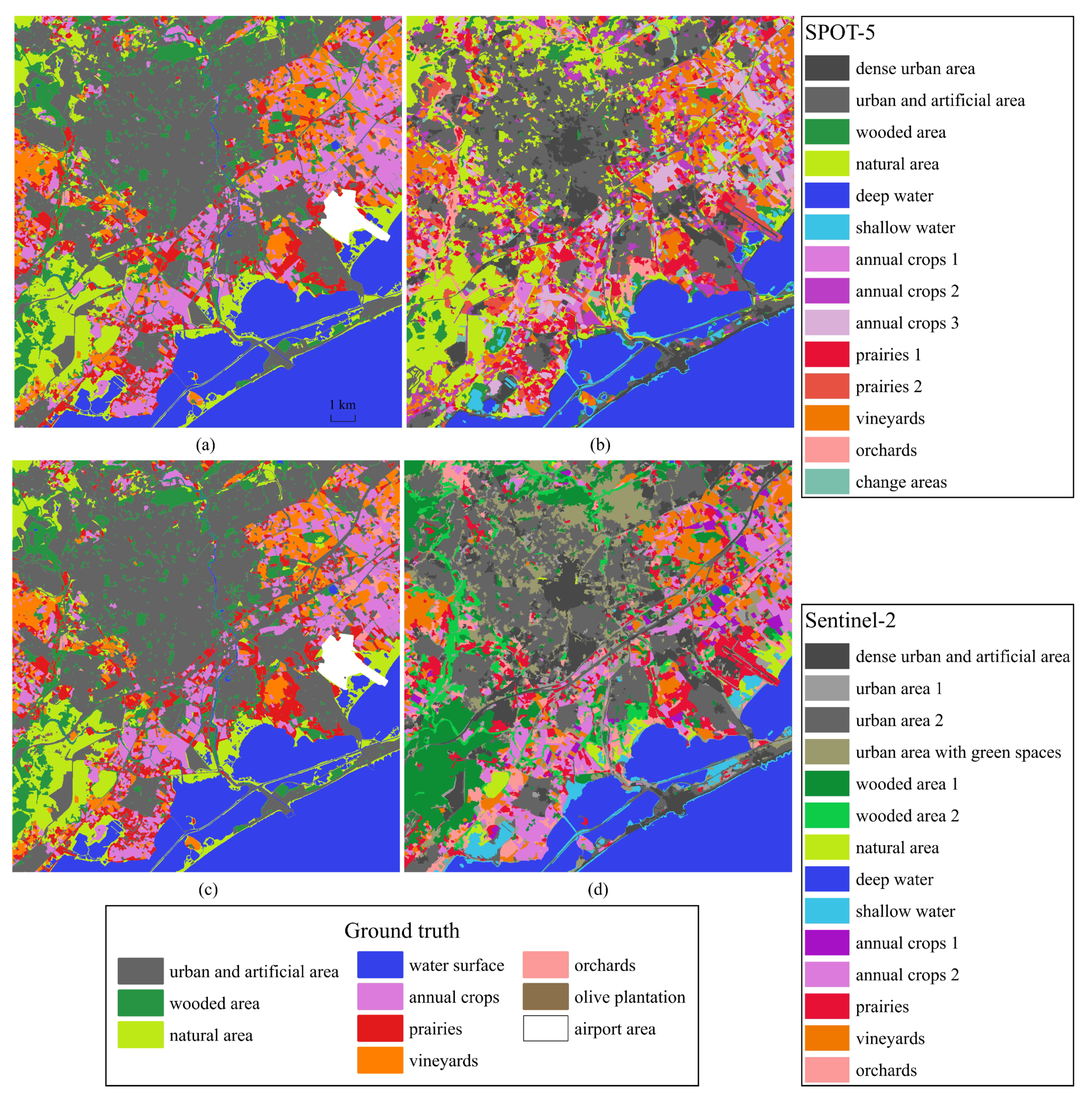
4.2.1. Quantitative Evaluation
4.2.2. Qualitative Evaluation. Segmentation
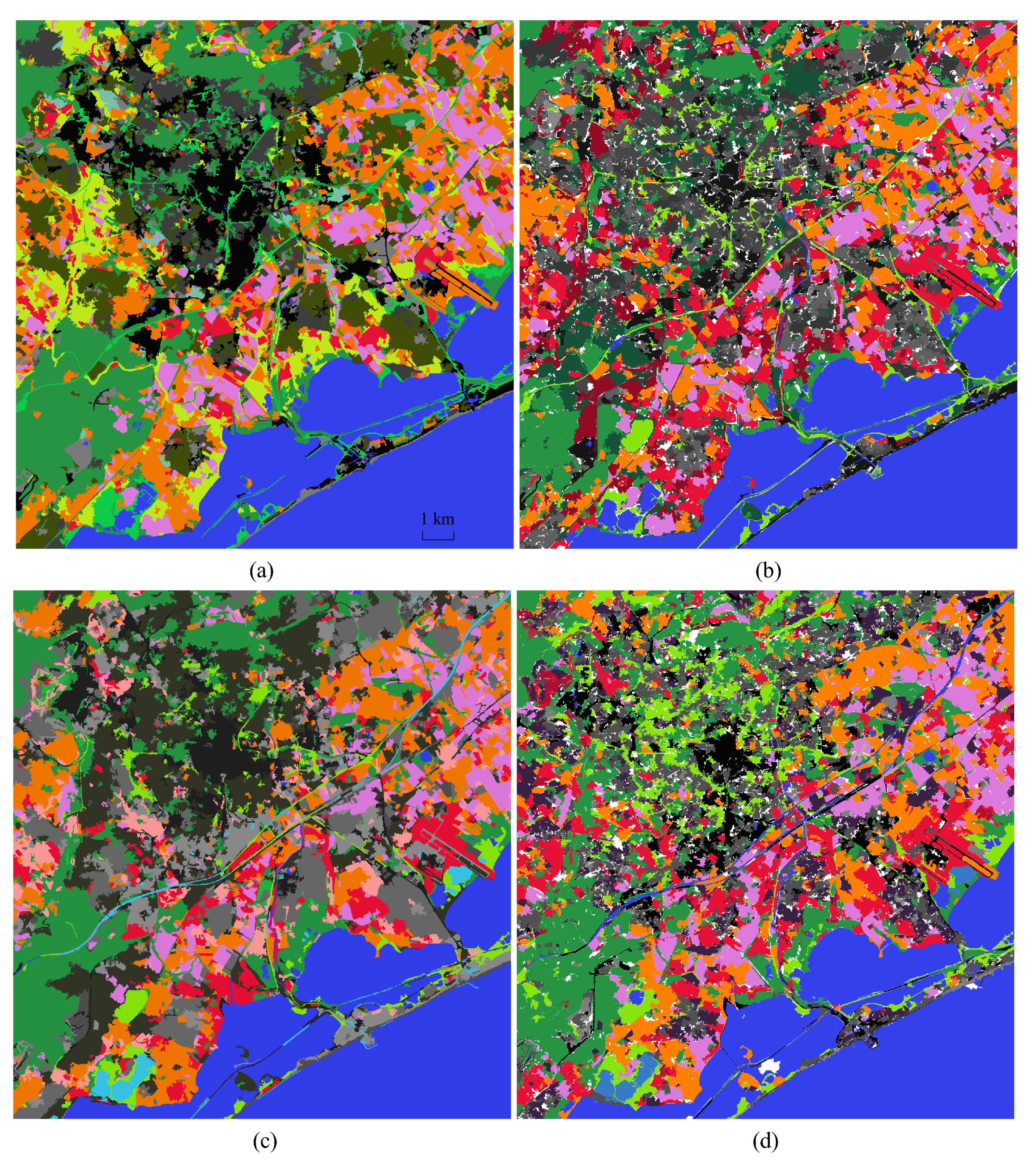
4.2.3. Qualitative Evaluation. Feature Extraction and Clustering
5. Conclusions
Author Contributions
Funding
Conflicts of Interest
Abbreviations
| SITS | Satellite Image Time Series |
| AE | AutoEncoder |
| NN | Neural Network |
| NMI | Normalized Mutual Information |
| DTW | Dynamic Time Warping |
| GT | Ground Truth |
| FC | Fully-Connected |
| NDVI | Normalized Difference Vegetation Index |
| FM | Feature Maps |
| OB | Object-based |
| GB | Graph-based |
References
- Nativi, S.; Mazzetti, P.; Santoro, M.; Papeschi, F.; Craglia, M.; Ochiai, O. Big Data challenges in building the Global Earth Observation System of Systems. Environ. Model. Softw. 2015, 68, 1–26. [Google Scholar] [CrossRef]
- Kuenzer, C.; Dech, S.; Wagner, W. Remote Sensing Time Series—Revealing Land Surface Dynamics; Springer: Berlin/Heidelberg, Germany, 2015; Volume 22. [Google Scholar] [CrossRef]
- Alqurashi, A.; Kumar, L.; Sinha, P. Urban Land Cover Change Modelling Using Time-Series Satellite Images: A Case Study of Urban Growth in Five Cities of Saudi Arabia. Remote. Sens. 2016, 8, 838. [Google Scholar] [CrossRef]
- Van Hoek, M.; Jia, L.; Zhou, J.; Zheng, C.; Menenti, M. Early Drought Detection by Spectral Analysis of Satellite Time Series of Precipitation and Normalized Difference Vegetation Index (NDVI). Remote. Sens. 2016, 8, 422. [Google Scholar] [CrossRef]
- Song, X.P.; Huang, C.; Sexton, J.O.; Channan, S.; Townshend, J.R. Annual Detection of Forest Cover Loss Using Time Series Satellite Measurements of Percent Tree Cover. Remote. Sens. 2014, 6, 8878–8903. [Google Scholar] [CrossRef]
- Kalinicheva, E.; Ienco, D.; Sublime, J.; Trocan, M. Unsupervised Change Detection Analysis in Satellite Image Time Series using Deep Learning Combined with Graph-Based Approaches. IEEE J. Sel. Top. Appl. Earth Obs. Remote. Sens. 2020. [Google Scholar] [CrossRef]
- Gómez, C.; White, J.C.; Wulder, M.A. Optical remotely sensed time series data for land cover classification: A review. ISPRS J. Photogramm. Remote. Sens. 2016, 116, 55–72. [Google Scholar] [CrossRef]
- Pelletier, C.; Webb, G.I.; Petitjean, F. Temporal Convolutional Neural Network for the Classification of Satellite Image Time Series. Remote. Sens. 2019, 11, 523. [Google Scholar] [CrossRef]
- Interdonato, R.; Ienco, D.; Gaetano, R.; Ose, K. DuPLO: A DUal view Point deep Learning architecture for time series classificatiOn. ISPRS J. Photogramm. Remote. Sens. 2019, 149, 91–104. [Google Scholar] [CrossRef]
- Petitjean, F.; Inglada, J.; Gancarski, P. Clustering of satellite image time series under Time Warping. In Proceedings of the 2011 6th International Workshop on the Analysis of Multi-temporal Remote Sensing Images (Multi-Temp), Trento, Italy, 12–14 July 2011; pp. 69–72. [Google Scholar] [CrossRef]
- Zhang, Z.; Tang, P.; Huo, L.; Zhou, Z. MODIS NDVI time series clustering under dynamic time warping. Int. J. Wavelets MultireSolut. Inf. Process. 2014, 12, 1461011. [Google Scholar] [CrossRef]
- Rakthanmanon, T.; Campana, B.; Mueen, A.; Batista, G.; Westover, M.B.; Zhu, Q.; Zakaria, J.; Keogh, E. Addressing Big Data Time Series: Mining Trillions of Time Series Subsequences Under Dynamic Time Warping. Acm Trans. Knowl. Discov. Data 2013, 7. [Google Scholar] [CrossRef]
- Belgiu, M.; Csillik, O. Sentinel-2 cropland mapping using pixel-based and object-based time-weighted dynamic time warping analysis. Remote. Sens. Environ. 2017, 204. [Google Scholar] [CrossRef]
- Csillik, O.; Belgiu, M.; Asner, G.; Kelly, M. Object-Based Time-Constrained Dynamic Time Warping Classification of Crops Using Sentinel-2. Remote. Sens. 2019, 11, 1257. [Google Scholar] [CrossRef]
- Petitjean, F.; Weber, J. Efficient Satellite Image Time Series Analysis Under Time Warping. IEEE Geosci. Remote. Sens. Lett. 2014, 11, 1143–1147. [Google Scholar] [CrossRef]
- Petitjean, F.; Kurtz, C.; Passat, N.; Gancarski, P. Spatio-Temporal Reasoning for the Classification of Satellite Image Time Series. Pattern Recognit. Lett. 2013, 33, 1805. [Google Scholar] [CrossRef]
- Guttler, F.; Ienco, D.; Nin, J.; Teisseire, M.; Poncelet, P. A graph-based approach to detect spatiotemporal dynamics in satellite image time series. ISPRS J. Photogramm. Remote. Sens. 2017, 130, 92–107. [Google Scholar] [CrossRef]
- Khiali, L.; Ndiath, M.; Alleaume, S.; Ienco, D.; Ose, K.; Teisseire, M. Detection of spatio-temporal evolutions on multi-annual satellite image time series: A clustering based approach. Int. J. Appl. Earth Obs. Geoinf. 2019, 74, 103–119. [Google Scholar] [CrossRef]
- Costa, W.; Fonseca, L.; Körting, T.; Simoes, M.; Kuchler, P. A Case Study for a Multitemporal Segmentation Approach in Optical Remote Sensing Images. In Proceedings of 10th International Conference on Advanced Geographic Information Systems, Applications, and Services; Israel Institute of Technology: Haifa, Israel, 2018; pp. 66–70. [Google Scholar]
- Ji, S.; Chi, Z.; Xu, A.; Duan, Y. 3D Convolutional Neural Networks for Crop Classification with Multi-Temporal Remote Sensing Images. Remote. Sens. 2018, 10, 75. [Google Scholar] [CrossRef]
- Li, Y.; Zhang, H.; Shen, Q. Spectral–Spatial Classification of Hyperspectral Imagery with 3D Convolutional Neural Network. Remote. Sens. 2017, 9, 67. [Google Scholar] [CrossRef]
- Shi, X.; Chen, Z.; Wang, H.; Yeung, D.; Wong, W.; Woo, W. Convolutional LSTM Network: A Machine Learning Approach for Precipitation Nowcasting. arXiv 2015, arXiv:1506.04214. [Google Scholar]
- Goodfellow, I.; Bengio, Y.; Courville, A. Deep Learning; Adaptive Computation and Machine Learning Series; Chapter Autoencoders; MIT Press: Cambridge, MA, USA, 2016. [Google Scholar]
- Xing, C.; Ma, L.; Yang, X. Stacked Denoise Autoencoder Based Feature Extraction and Classification for Hyperspectral Images. J. Sens. 2016, 2016, 1–10. [Google Scholar] [CrossRef]
- Cui, W.; Zhou, Q. Application of a Hybrid Model Based on a Convolutional Auto-Encoder and Convolutional Neural Network in Object-Oriented Remote Sensing Classification. Algorithms 2018, 11, 9. [Google Scholar] [CrossRef]
- Liang, P.; Shi, W.; Zhang, X. Remote Sensing Image Classification Based on Stacked Denoising Autoencoder. Remote. Sens. 2017, 10, 16. [Google Scholar] [CrossRef]
- Rouse, J.W.; Haas, R.H.; Schell, J.A.; Deering, D.W. Monitoring Vegetation Systems in the Great Plains with Erts; NASA Special Publication: Washington, DC, USA, 1974; Volume 351, p. 309.
- Ward, J.H., Jr. Hierarchical Grouping to Optimize an Objective Function. J. Am. Stat. Assoc. 1963, 58, 236–244. [Google Scholar] [CrossRef]
- El Hajj, M.; Bégué, A.; Lafrance, B.; Hagolle, O.; Dedieu, G.; Rumeau, M. Relative Radiometric Normalization and Atmospheric Correction of a SPOT 5 Time Series. Sensors 2008, 8, 2774–2791. [Google Scholar] [CrossRef]
- Tran, D.; Bourdev, L.; Fergus, R.; Torresani, L.; Paluri, M. Learning Spatiotemporal Features with 3D Convolutional Networks. In Proceedings of the 2015 IEEE International Conference on Computer Vision (ICCV), Santiago, Chile, 7–13 December 2015; pp. 4489–4497. [Google Scholar] [CrossRef]
- Fukunaga, K.; Hostetler, L. The estimation of the gradient of a density function, with applications in pattern recognition. IEEE Trans. Inf. Theory 1975, 21, 32–40. [Google Scholar] [CrossRef]
- Tavenard, R.; Faouzi, J.; Vandewiele, G.; Divo, F.; Androz, G.; Holtz, C.; Payne, M.; Yurchak, R.; Rußwurm, M.; Kolar, K.; et al. Tslearn: A Machine Learning Toolkit Dedicated to Time-Series Data. 2017. Available online: https://github.com/rtavenar/tslearn (accessed on 1 May 2020).
- Cover, T.M.; Thomas, J.A. Elements of Information Theory (Wiley Series in Telecommunications and Signal Processing); Wiley-Interscience: Hoboken, NJ, USA, 2006. [Google Scholar]
- Sakoe, H.; Chiba, S. Dynamic programming algorithm optimization for spoken word recognition. IEEE Trans. Acoust. Speech Signal Process. 1978, 26, 43–49. [Google Scholar] [CrossRef]
Sample Availability: The source code and image results are available from the authors and in the repository https://github.com/ekalinicheva/3D_SITS_Clustering/. |


| Acquisition Date, yyyy-mm-dd | |||
|---|---|---|---|
| 1 | 2002-10-05 | 7 | 2006-02-18 |
| 2 | 2003-09-18 | 8 | 2006-06-03 |
| 3 | 2004-05-14 | 9 | 2007-02-01 |
| 4 | 2004-08-22 | 10 | 2007-04-06 |
| 5 | 2005-04-27 | 11 | 2008-06-21 |
| 6 | 2005-12-01 | 12 | 2008-08-21 |
| Acquisition Date, yyyy-mm-dd | |||||||
|---|---|---|---|---|---|---|---|
| 1 | 2017-01-03 | 7 | 2017-08-20 | 13 | 2017-12-19 | 19 | 2018-07-17 |
| 2 | 2017-03-14 | 8 | 2017-09-20 | 14 | 2018-01-23 | 20 | 2018-08-06 |
| 3 | 2017-04-03 | 9 | 2017-10-10 | 15 | 2018-02-12 | 21 | 2018-08-26 |
| 4 | 2017-04-23 | 10 | 2017-10-30 | 16 | 2018-02-27 | 22 | 2018-09-20 |
| 5 | 2017-06-12 | 11 | 2017-11-14 | 17 | 2018-04-18 | 23 | 2018-10-05 |
| 6 | 2017-07-12 | 12 | 2017-11-29 | 18 | 2018-06-27 | 24 | 2018-12-29 |
| Dataset | Parameters | ||
|---|---|---|---|
| Rs | Rr | Omin | |
| SPOT-5 | 45 | 40 | 10 |
| Sentinel-2 | 40 | 35 | 10 |
| SPOT-5 | SPOT-5 w/o Outliers | Sentinel-2 | ||||
|---|---|---|---|---|---|---|
| NMI | NMI Best | NMI | NMI Best | NMI | NMI Best | |
| Our method | 0.45 ± 0.01 | 0.45 ± 0.01 | 0.5 ± 0.01 | 0.5 ± 0.01 | 0.44 ± 0.01 | 0.45 ± 0.01 |
| OB DTW | 0.4 | 0.4 | 0.43 | 0.46 | 0.36 | 0.38 |
| OB DTW + NDVI | 0.41 | 0.41 | 0.44 | 0.44 | 0.36 | 0.37 |
| GB DTW | 0.36 | 0.38 | 0.37 | 0.39 | 0.36 | 0.36 |
| GB DTW + NDVI | 0.41 | 0.42 | 0.42 | 0.42 | 0.37 | 0.37 |
| AE w/o NDVI | 0.45 ± 0.01 | 0.46 ± 0 | 0.48 ± 0.02 | 0.48 ± 0.02 | 0.43 ± 0.01 | 0.43 ± 0.01 |
| AE w/o segm. corr. | 0.42 ± 0.01 | 0.42 ± 0.01 | 0.47 ± 0 | 0.47 ± 0 | 0.43 ± 0.01 | 0.43 ± 0.01 |
| Our method + GT seg. | 0.52 ± 0.01 | 0.52 ± 0.01 | 0.58 ± 0.01 | 0.59 ± 0 | 0.46 ± 0.05 | 0.5 ± 0.01 |
| OB DTW + GT seg. | 0.51 | 0.53 | 0.52 | 0.54 | 0.48 | 0.48 |
| OB DTW + GT seg. + NDVI | 0.52 | 0.53 | 0.54 | 0.54 | 0.4 | 0.45 |
| Algorithm Step | Computation Time, Min | ||
|---|---|---|---|
| SPOT-5 | Sentinel-2 | ||
| Our method | Model training a + encoding | 15 + 5 | 25 + 6 |
| AE w/o NDVI | Model training a + encoding | 11 + 3 | 15 + 4 |
| OB DTW | DTW calc. b | 35 (4433 objects) | 30 (3751 objects) |
| OB DTW + NDVI | DTW calc. b | 40 (4433 objects) | 33 (3751 objects) |
| GB DTW | Graph constr. + DTW calc. b | 26 + 33 (3550 graphs) | 55 + 51 (3739 graphs) |
| GB DTW + NDVI | Graph constr. + DTW calc. b | 26 + 36 (3550 graphs) | 55 + 56 (3739 graphs) |
| OB DTW + GT seg. | DTW calc. b | 202 (10,725 objects) | 299 (12,236 objects) |
| OB DTW + GT seg. + NDVI | DTW calc. b | 232 (10,725 objects) | 335 (12,236 objects) |
© 2020 by the authors. Licensee MDPI, Basel, Switzerland. This article is an open access article distributed under the terms and conditions of the Creative Commons Attribution (CC BY) license (http://creativecommons.org/licenses/by/4.0/).
Share and Cite
Kalinicheva, E.; Sublime, J.; Trocan, M. Unsupervised Satellite Image Time Series Clustering Using Object-Based Approaches and 3D Convolutional Autoencoder. Remote Sens. 2020, 12, 1816. https://doi.org/10.3390/rs12111816
Kalinicheva E, Sublime J, Trocan M. Unsupervised Satellite Image Time Series Clustering Using Object-Based Approaches and 3D Convolutional Autoencoder. Remote Sensing. 2020; 12(11):1816. https://doi.org/10.3390/rs12111816
Chicago/Turabian StyleKalinicheva, Ekaterina, Jérémie Sublime, and Maria Trocan. 2020. "Unsupervised Satellite Image Time Series Clustering Using Object-Based Approaches and 3D Convolutional Autoencoder" Remote Sensing 12, no. 11: 1816. https://doi.org/10.3390/rs12111816
APA StyleKalinicheva, E., Sublime, J., & Trocan, M. (2020). Unsupervised Satellite Image Time Series Clustering Using Object-Based Approaches and 3D Convolutional Autoencoder. Remote Sensing, 12(11), 1816. https://doi.org/10.3390/rs12111816