Detailed Lacustrine Calving Iceberg Inventory from Very High Resolution Optical Imagery and Object-Based Image Analysis


Abstract
1. Introduction
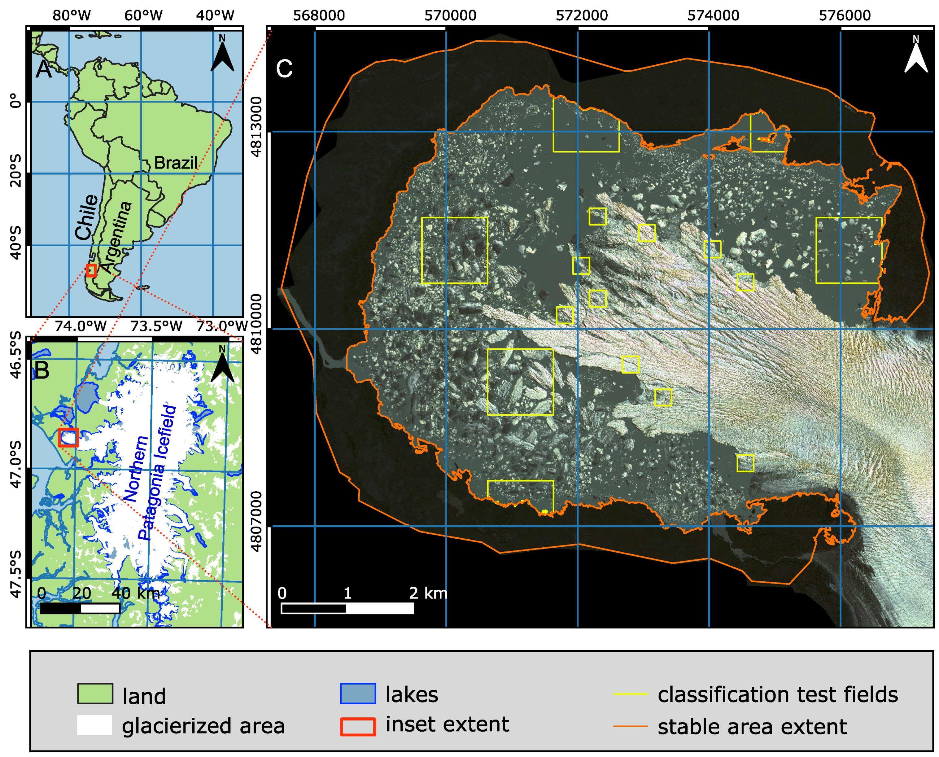
2. Study Area
3. Data and Methods
3.1. Datasets Used and Imagery Preprocessing
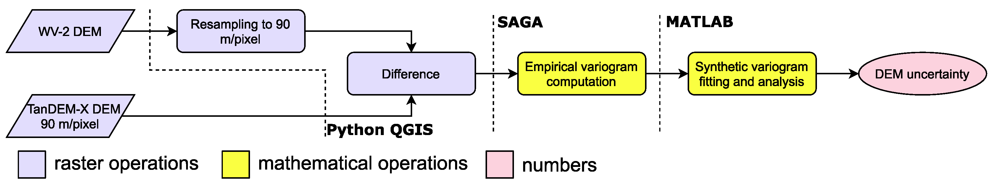
3.2. DEM Preprocessing
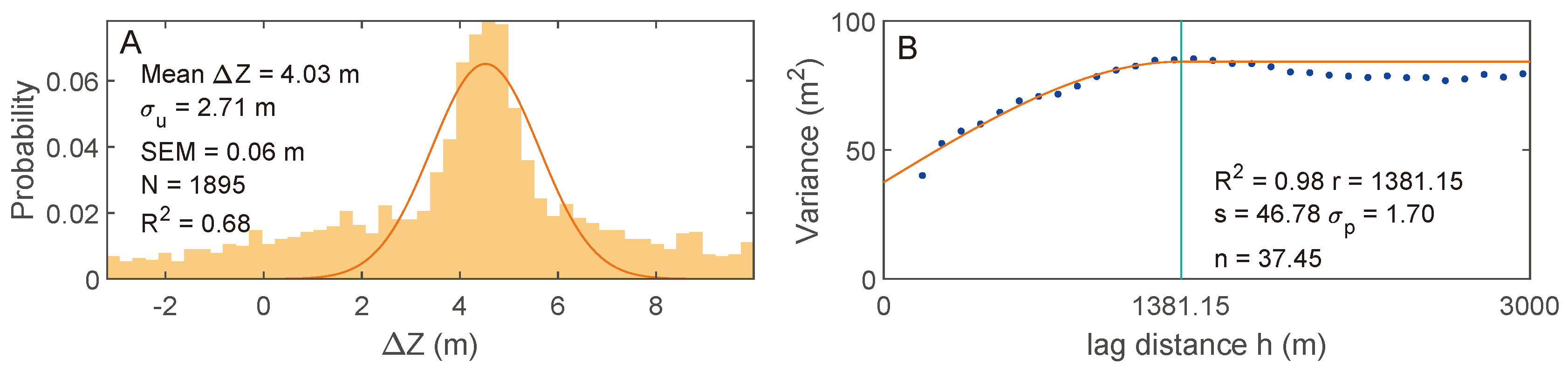
3.3. DEM Uncertainty Assessment
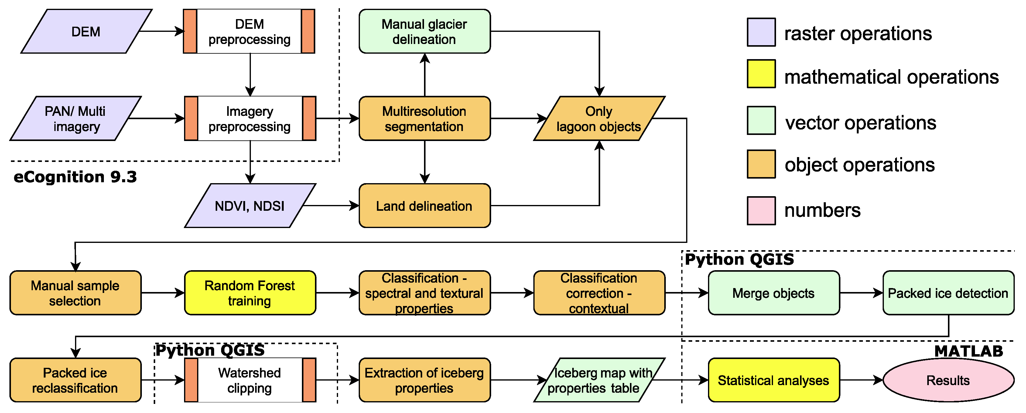
3.4. Iceberg Map Creation
3.5. Iceberg Map Uncertainty Assessment
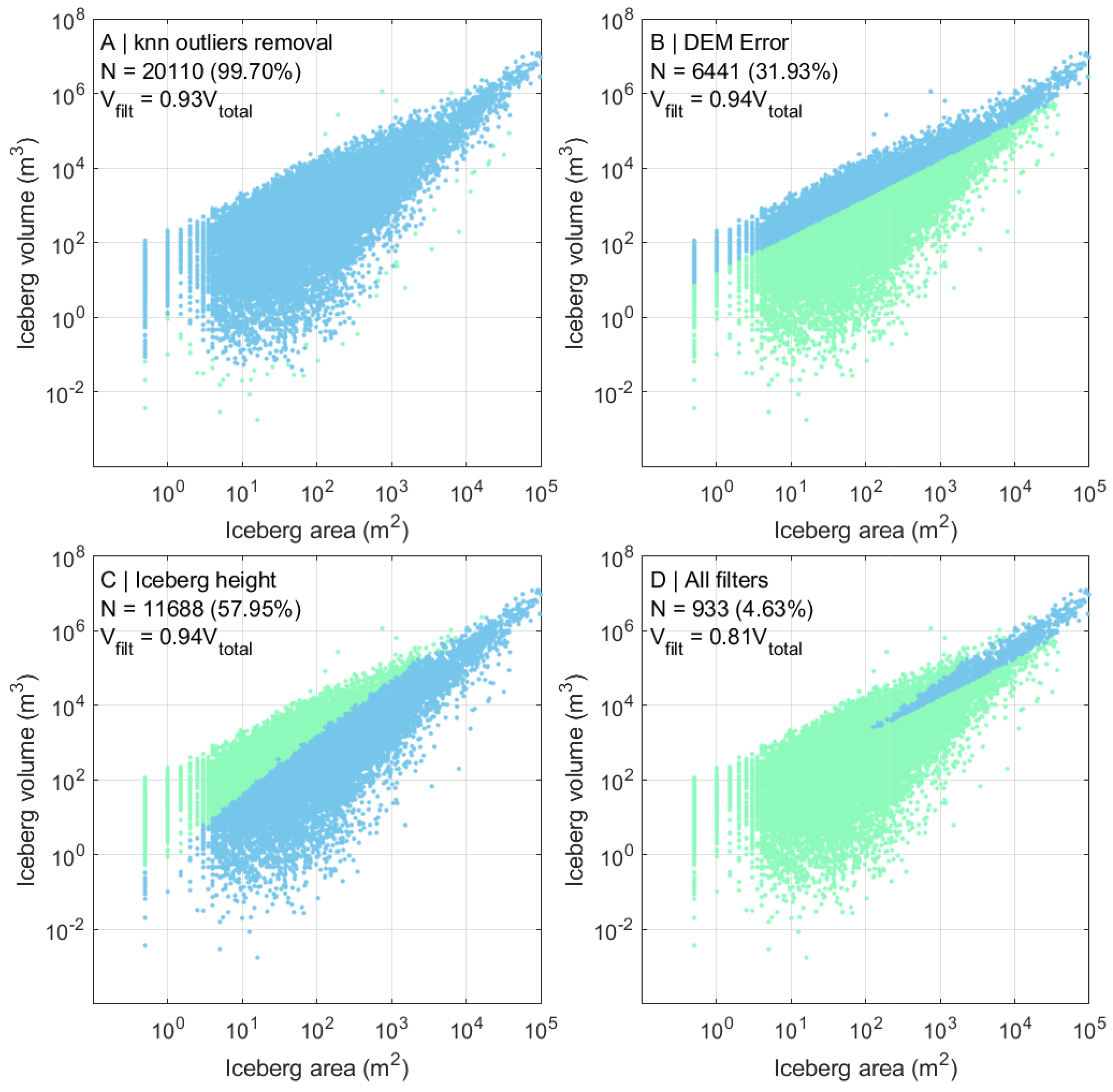
3.6. Data Filtering
- We used k-nearest neighbors (knn) clustering algorithm to discard outlying data points. All items which had fewer than four neighbors within radius of 0.2 in the log area–log volume space were considered outliers.
- All icebergs with were discarded. We assumed objects to be unreliable when their elevation measurements are below the precision of the DREM.
- We filtered out icebergs which were unrealistically high with respect to their width. We used a formula proposed in [48] (Equation (6)) for the critical width/height ratio at which an iceberg capsizes. We assumed that any iceberg with width/height below the critical ratio should capsize and thus the elevation measurement is not realistic.where is the critical ratio, equal to under our assumed ice and water densities.
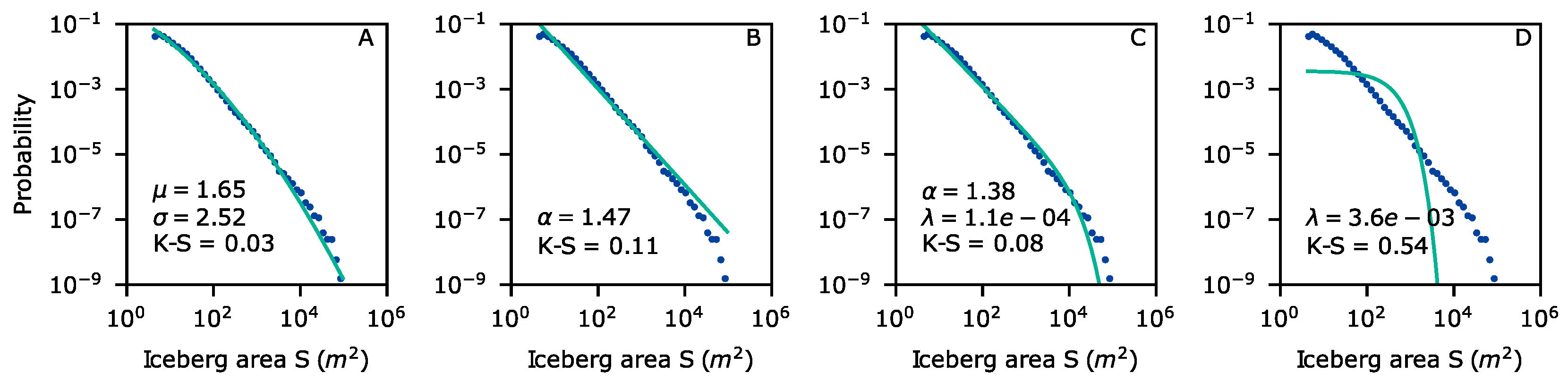
3.7. Area and Volume Distribution
3.8. Area–Volume Scaling
- of the fit; and
- —the product of k-fold cross-validation (CV) of a model. We divided the area–volume dataset into 10 subsets (folds) and performed the fitting with 9 subsets leaving one of them out for verification. of the volumes computed with the fitted line vs. the measured volumes was computed at each of the repetitions and the mean of these s is reported as .
4. Results
4.1. DEM Accuracy Assessment
4.2. Dataset and Filtering
4.3. Classification Accuracy Assessment
4.4. Area and Volume Distribution
4.5. Area–Volume Scaling
5. Discussion
5.1. Iceberg Classification
5.2. Iceberg Inventory
5.3. Volume Assessment
5.4. Area–Volume Scaling and Distributions
6. Conclusions
Author Contributions
Acknowledgments
Conflicts of Interest
Appendix A

| Processing Step | Tool | Input Data | Flowchart |
|---|---|---|---|
| WV-2 imagery preprocessing | ENVI 5 | WV-2 raw images | Figure 2 |
| DREM creation | QGIS 3.10 | WV-2 DEM | Figure 3 |
| DREM uncertainty assessment | QGIS 3.10, SAGA, MATLAB | WV-2 DEM, TanDEM-X DEM | Figure 4 |
| Image segmentation and classification | eCognition 9.3 | WV-2 processed images, DREM | Figure 5 |
| Watershed cutting | Python 3 | Shapefile map of icebergs | Figure 6 |
| Iceberg detection quality assessment | MATLAB | Cut shapefile map of icebergs | - |
| Iceberg properties extraction | eCognition 9.3 | Cut shapefile map of icebergs | Figure 5 |
| Statistical analysis | MATLAB | Table of iceberg properties | - |
References
- Warren, C.; Benn, D.; Winchester, V.; Harrison, S. Buoyancy-driven lacustrine calving, Glaciar Nef, Chilean Patagonia. J. Glaciol. 2001, 47, 135–146. [Google Scholar] [CrossRef]
- Benn, D.I.; Warren, C.R.; Mottram, R.H. Calving processes and the dynamics of calving glaciers. Earth-Sci. Rev. 2007, 82, 143–179. [Google Scholar] [CrossRef]
- Trüssel, B.L.; Motyka, R.J.; Truffer, M.; Larsen, C.F. Rapid thinning of lake-calving Yakutat Glacier and the collapse of the Yakutat Icefield, southeast Alaska, USA. J. Glaciol. 2013, 59, 149–161. [Google Scholar] [CrossRef]
- Loriaux, T.; Casassa, G. Evolution of glacial lakes from the Northern Patagonia Icefield and terrestrial water storage in a sea-level rise context. Glob. Planet. Chang. 2013, 102, 33–40. [Google Scholar] [CrossRef]
- Schoolmeester, T. The Andean Glacier and Water Atlas: The Impact of Glacier Retreat on Water Resources; UNESCO GRID-Arenal: Paris, France; Arendal, Norway, 2018. [Google Scholar]
- Mazur, A.; Wåhlin, A.; Krężel, A. An object-based SAR image iceberg detection algorithm applied to the Amundsen Sea. Remote Sens. Environ. 2017, 189, 67–83. [Google Scholar] [CrossRef]
- Soldal, I.; Dierking, W.; Korosov, A.; Marino, A. Automatic Detection of Small Icebergs in Fast Ice Using Satellite Wide-Swath SAR Images. Remote Sens. 2019, 11, 806. [Google Scholar] [CrossRef]
- Neuhaus, S.U.; Tulaczyk, S.M.; Begeman, C.B. Spatiotemporal distributions of icebergs in a temperate fjord: Columbia Fjord, Alaska. Cryosphere 2019, 13, 1785–1799. [Google Scholar] [CrossRef]
- Scheick, J.; Enderlin, E.M.; Hamilton, G. Semi-automated open water iceberg detection from Landsat applied to Disko Bay, West Greenland. J. Glaciol. 2019, 65, 468–480. [Google Scholar] [CrossRef]
- Köhler, A.; Pętlicki, M.; Lefeuvre, P.M.; Buscaino, G.; Nuth, C.; Weidle, C. Contribution of calving to frontal ablation quantified from seismic and hydroacoustic observations calibrated with lidar volume measurements. Cryosphere 2019, 13, 3117–3137. [Google Scholar] [CrossRef]
- Minowa, M.; Podolskiy, E.A.; Sugiyama, S.; Sakakibara, D.; Skvarca, P. Glacier calving observed with time-lapse imagery and tsunami waves at Glaciar Perito Moreno, Patagonia. J. Glaciol. 2018, 64, 362–376. [Google Scholar] [CrossRef]
- Mallalieu, J.; Carrivick, J.L.; Quincey, D.J.; Smith, M.W. Calving Seasonality Associated with Melt-Undercutting and Lake Ice Cover. Geophys. Res. Lett. 2020, 47. [Google Scholar] [CrossRef]
- Dowdeswell, J.A.; Forsberg, C.F. The size and frequency of icebergs and bergy bits derived from tidewater glaciers in Kongsfjorden, northwest Spitsbergen. Polar Res. 1992, 11, 81–91. [Google Scholar] [CrossRef]
- Tournadre, J.; Bouhier, N.; Girard-Ardhuin, F.; Rémy, F. Antarctic icebergs distributions 1992–2014. J. Geophys. Res. Ocean. 2016, 121, 327–349. [Google Scholar] [CrossRef]
- Kirkham, J.D.; Rosser, N.J.; Wainwright, J.; Jones, E.C.V.; Dunning, S.A.; Lane, V.S.; Hawthorn, D.E.; Strzelecki, M.C.; Szczuciński, W. Drift-dependent changes in iceberg size-frequency distributions. Sci. Rep. 2017, 7, 1–10. [Google Scholar] [CrossRef]
- Crocker, G. Size distributions of bergy bits and growlers calved from deteriorating icebergs. Cold Reg. Sci. Technol. 1993, 22, 113–119. [Google Scholar] [CrossRef]
- Stern, A.A.; Adcroft, A.; Sergienko, O. The effects of Antarctic iceberg calving-size distribution in a global climate model. J. Geophys. Res. Ocean. 2016, 121, 5773–5788. [Google Scholar] [CrossRef]
- Sulak, D.J.; Sutherland, D.A.; Enderlin, E.M.; Stearns, L.A.; Hamilton, G.S. Iceberg properties and distributions in three Greenlandic fjords using satellite imagery. Ann. Glaciol. 2017, 58, 92–106. [Google Scholar] [CrossRef]
- Blaschke, T.; Hay, G.J.; Kelly, M.; Lang, S.; Hofmann, P.; Addink, E.; Feitosa, R.Q.; van der Meer, F.; van der Werff, H.; van Coillie, F.; et al. Geographic Object-Based Image Analysis—Towards a new paradigm. ISPRS J. Photogramm. Remote Sens. 2014, 87, 180–191. [Google Scholar] [CrossRef]
- Rastner, P.; Bolch, T.; Notarnicola, C.; Paul, F. A Comparison of Pixel- and Object-Based Glacier Classification With Optical Satellite Images. IEEE J. Sel. Top. Appl. Earth Obs. Remote Sens. 2014, 7, 853–862. [Google Scholar] [CrossRef]
- Robson, B.A.; Nuth, C.; Dahl, S.O.; Hölbling, D.; Strozzi, T.; Nielsen, P.R. Automated classification of debris-covered glaciers combining optical, SAR and topographic data in an object-based environment. Remote Sens. Environ. 2015, 170, 372–387. [Google Scholar] [CrossRef]
- Jawak, S.D.; Wankhede, S.F.; Luis, A.J. Exploration of Glacier Surface Facies Mapping Techniques Using Very High Resolution Worldview-2 Satellite Data. Proceedings 2018, 2, 339. [Google Scholar] [CrossRef]
- Mitkari, K.V.; Arora, M.K.; Tiwari, R.K. Extraction of Glacial Lakes in Gangotri Glacier Using Object-Based Image Analysis. IEEE J. Sel. Top. Appl. Earth Obs. Remote Sens. 2017, 10, 5275–5283. [Google Scholar] [CrossRef]
- McNabb, R.W.; Womble, J.N.; Prakash, A.; Gens, R.; Haselwimmer, C.E. Quantification and Analysis of Icebergs in a Tidewater Glacier Fjord Using an Object-Based Approach. PLoS ONE 2016, 11, e0164444. [Google Scholar] [CrossRef] [PubMed]
- Aniya, M.; Enomoto, H. Glacier Variations and Their Causes in the Northern Patagonia Icefield, Chile, Since 1944. Arct. Alp. Res. 1986, 18, 307. [Google Scholar] [CrossRef]
- Le Bris, R.; Paul, F.; Rastner, P.; Schaub, Y. GLIMS Glacier Database; National Snow and Ice Data Center: Boulder, CO, USA, 2018. [Google Scholar]
- Harrison, S.; Warren, C.R.; Winchester, V.; Aniya, M. Onset of rapid calving and retreat of Glaciar San Quintin, Hielo Patagónico Norte, southern Chile. Polar Geogr. 2001, 25, 54–61. [Google Scholar] [CrossRef]
- Aniya, M. Glacier variations of Hielo Patagónico Norte, Chile, over 70 years from 1945 to 2015. Bull. Glaciol. Res. 2017, 35, 19–38. [Google Scholar] [CrossRef]
- Di Tullio, M.; Nocchi, F.; Camplani, A.; Emanuelli, N.; Nascetti, A.; Crespi, M. Copernicus Big Data And Google Earth Engine For Glacier Surface Velocity Field Monitoring: Feasibility Demonstration on San Rafael and San Quintin Glaciers. ISPRS-Int. Arch. Photogramm. Remote Sens. Spat. Inf. Sci. 2018, XLII-3, 289–294. [Google Scholar] [CrossRef]
- Dixon, L.; Ambinakudige, S. Remote Sensing Study of Glacial Change in the Northern Patagonian Icefield. Adv. Remote Sens. 2015, 4, 270–279. [Google Scholar] [CrossRef][Green Version]
- DigitalGlobe. Base Product Series FAQ. 2016. Available online: https://www.c-agg.org/wp-content/uploads/DigitalGlobe-Base-Product-FAQ.pdf (accessed on 9 April 2020).
- Eisank, C.; Rieg, L.; Klug, C.; Kleindienst, H.; Sailer, R. Semi-Global Matching of Pléiades Tri-Stereo Imagery to Generate Detailed Digital Topography for High-Alpine Regions. GI_Forum 2015, 1, 168–177. [Google Scholar] [CrossRef]
- Rizzoli, P.; Martone, M.; Gonzalez, C.; Wecklich, C.; Tridon, D.B.; Bräutigam, B.; Bachmann, M.; Schulze, D.; Fritz, T.; Huber, M.; et al. Generation and performance assessment of the global TanDEM-X digital elevation model. ISPRS J. Photogramm. Remote Sens. 2017, 132, 119–139. [Google Scholar] [CrossRef]
- Wessel, B.; Huber, M.; Wohlfart, C.; Marschalk, U.; Kosmann, D.; Roth, A. Accuracy assessment of the global TanDEM-X Digital Elevation Model with GPS data. ISPRS J. Photogramm. Remote Sens. 2018, 139, 171–182. [Google Scholar] [CrossRef]
- DigitalGlobe. WorldView-2 Data Sheet and Core Imagery Product Guide. 2016. Available online: https://dg-cms-uploads-production.s3.amazonaws.com/uploads/document/file/98/WorldView2-DS-WV2-rev2.pdf (accessed on 9 April 2020).
- Hall, D.K.; Riggs, G.A. Normalized-Difference Snow Index (NDSI). In Encyclopedia of Snow, Ice and Glaciers; Singh, V.P., Singh, P., Haritashya, U.K., Eds.; Springer: Amsterdam, The Netherlands, 2011; pp. 779–780. [Google Scholar]
- Haala, N.; Rothermel, M. Dense Multi-Stereo Matching for High Quality Digital Elevation Models. Photogramm. Fernerkund. Geoinf. 2012, 2012, 331–343. [Google Scholar] [CrossRef]
- Podgórski, J.; Kinnard, C.; Pętlicki, M.; Urrutia, R. Performance Assessment of TanDEM-X DEM for Mountain Glacier Elevation Change Detection. Remote Sens. 2019, 11, 187. [Google Scholar] [CrossRef]
- Rolstad, C.; Haug, T.; Denby, B. Spatially integrated geodetic glacier mass balance and its uncertainty based on geostatistical analysis: Application to the western Svartisen ice cap, Norway. J. Glaciol. 2009, 55, 666–680. [Google Scholar] [CrossRef]
- Trimble Geospatial. Trimble eCognition Suite for Windows Operating System. 2017. Available online: http://www.infoserve.co.jp/doc/Trimble/v9_3/ReleaseNotes.pdf (accessed on 29 May 2020).
- Rouse, J.W., Jr.; Haas, R.H.; Schell, J.A.; Deering, D.W. Monitoring vegetation systems in the Great Plains with ERTS. In Goddard Space Flight Center 3d ERTS-1 Symp. Sect. A; Freden, S.C., Mercanti, E.P., Becker, M.A., Eds.; NASA: Washington, DC, USA, 1974; Volume 1, pp. 309–317. [Google Scholar]
- Bradski, G. The OpenCV Library. Dr. Dobb’s J. Softw. Tools 2000. Available online: https://www.drdobbs.com/open-source/the-opencv-library/184404319 (accessed on 12 May 2020).
- OpenCV. OpenCV 2.4.13.7 Documentation. Random Trees. 2019. Available online: https://docs.opencv.org/2.4/modules/ml/doc/random_trees.html (accessed on 24 April 2020).
- Trimble Geospatial. In Trimble Documentation eCognition Developer 9.3 Reference Book; Trimble Germany GmbH: Munich, Germany, 2018.
- Beucher, S. Use of watersheds in contour detection. In Proceedings of the International Workshop on Image Processing (CCETT), Marne-la-Vallée, France, 26–28 March 1979. [Google Scholar]
- Mordvintsev, A.; Abid, K. Image Segmentation with Watershed Algorithm. In OpenCV 2.4.13.7 Documentation. 2013. Available online: https://opencv-python-tutroals.readthedocs.io/en/latest/py_tutorials/py_imgproc/py_watershed/py_watershed.html (accessed on 3 December 2019).
- Scheick, J.; Enderlin, E.; Miller, E.; Hamilton, G. First-Order Estimates of Coastal Bathymetry in Ilulissat and Naajarsuit Fjords, Greenland, from Remotely Sensed Iceberg Observations. Remote Sens. 2019, 11, 935. [Google Scholar] [CrossRef] [PubMed]
- Wagner, T.J.; Stern, A.A.; Dell, R.W.; Eisenman, I. On the representation of capsizing in iceberg models. Ocean Model. 2017, 117, 88–96. [Google Scholar] [CrossRef]
- Alstott, J.; Bullmore, E.; Plenz, D. powerlaw: A Python Package for Analysis of Heavy-Tailed Distributions. PLoS ONE 2014, 9, e85777. [Google Scholar] [CrossRef]
- Clauset, A.; Shalizi, C.R.; Newman, M.E.J. Power-Law Distributions in Empirical Data. SIAM Rev. 2009, 51, 661–703. [Google Scholar] [CrossRef]
- Bunting, P.; Clewley, D.; Lucas, R.M.; Gillingham, S. The Remote Sensing and GIS Software Library (RSGISLib). Comput. Geosci. 2014, 62, 216–226. [Google Scholar] [CrossRef]
- Truffer, M.; Motyka, R.J. Where glaciers meet water: Subaqueous melt and its relevance to glaciers in various settings. Rev. Geophys. 2016, 54, 220–239. [Google Scholar] [CrossRef]
- Larsen, C.F.; Motyka, R.J.; Arendt, A.A.; Echelmeyer, K.A.; Geissler, P.E. Glacier changes in southeast Alaska and northwest British Columbia and contribution to sea level rise. J. Geophys. Res. 2007, 112. [Google Scholar] [CrossRef]


| Band | Wavelength | Original Resolution | Date | Source |
|---|---|---|---|---|
| Blue | 450–510 nm | 2 m/pixel | 17 February 2017 | [35] |
| Green | 510–580 nm | |||
| Red | 630–690 nm | |||
| NIR | 770–895 nm | |||
| Panchromatic | 450–800 nm | 0.5 m/pixel | ||
| WV-2 DEM | Elevation | 2 m/pixel | 17 February 2017 | |
| TanDEM-X DEM | Elevation | 90 m/pixel | 22 January 2011–8 September 2014 | [33,34] |
| Class | Interpretation | Visible Brightness | Relative Elevation | Texture | Comments |
|---|---|---|---|---|---|
| Clear Ice | Ice without debris cover | Very bright | Positive | Uniform to moderately grainy | — |
| Dirty Ice | Icebergs or their sections covered with debris | Low, moderately variable | Positive | Non-uniform due to variable amount of debris | Easily mistaken for brash ice |
| Brash Ice | Fields of icebergs too small to be resolved individually | Moderately bright | Close to 0 | Very highly textured | Easily mistaken for dirty ice due to similar brightness |
| Shadow | Areas in deep shadow cast by an iceberg or glacier | Extremely low | Variable, depends on location | Very uniform | “Technical” class, merged with other classes in postprocessing |
| Water | Open water area, without ice | Narrow band of brightness | 0 | Very uniform | Brightness values within range of Dirty and Brash Ice |
| Big Iceberg | Tabular icebergs trapped in tightly packed ice melange | Variable, from clear ice to very dark | Very high | Variable, mostly uniform | Only used to reclassify the ice melange region |
| Small Iceberg | Small icebergs trapped in tightly packed melange | Moderately bright, with very bright pieces of clear ice | Variable, positive, close to 0 | Uniform within small objects | Only used to reclassify the ice melange region |
| Image Object Property | RF imp. | Parameter Loadings | |||
|---|---|---|---|---|---|
| PC1 | PC2 | PC3 | PC4 | ||
| Border contrast Panchromatic band | 0.024 | 0.08 | 0.07 | 0.68 | 0.17 |
| GLCM Contrast | 0.030 | 0.06 | −0.27 | 0.22 | 0.77 |
| GLCM Entropy | 0.032 | 0.00 | 0.00 | 0.00 | 0.00 |
| GLCM Homogeneity | 0.029 | 0.00 | 0.00 | 0.00 | 0.00 |
| GLCM Mean | 0.047 | 0.03 | 0.01 | 0.01 | −0.02 |
| Max. relative elevation | 0.031 | 0.00 | 0.00 | 0.00 | −0.01 |
| Max. Green band reflectance | 0.053 | 0.29 | −0.29 | −0.20 | −0.04 |
| Max. Panchromatic band reflectance | 0.052 | 0.42 | −0.38 | −0.11 | 0.00 |
| Max. Red band reflectance | 0.045 | 0.28 | −0.27 | −0.14 | −0.02 |
| Max. NDSI value | 0.025 | 0.00 | 0.00 | 0.00 | 0.00 |
| Max. Blue band reflectance | 0.052 | 0.28 | −0.27 | −0.21 | −0.03 |
| Mean Blue band reflectance | 0.069 | 0.26 | 0.08 | 0.12 | −0.13 |
| Mean relative elevation | 0.044 | 0.00 | 0.00 | 0.00 | −0.01 |
| Mean Green band reflectance | 0.066 | 0.28 | 0.07 | 0.13 | −0.14 |
| Mean NDSI value | 0.027 | 0.00 | 0.00 | 0.00 | 0.00 |
| Mean NIR band reflectance | 0.027 | 0.17 | 0.09 | 0.20 | −0.17 |
| Mean Panchromatic band reflectance | 0.023 | 0.40 | 0.14 | 0.29 | −0.20 |
| Mean Red band reflectance | 0.035 | 0.27 | 0.11 | 0.21 | −0.13 |
| Min. NDSI value | 0.024 | 0.00 | 0.00 | 0.00 | 0.00 |
| Min. Panchromatic band reflectance | 0.028 | 0.27 | 0.46 | −0.17 | 0.22 |
| Min. relative elevation | 0.024 | 0.00 | 0.00 | 0.00 | 0.00 |
| Min. Blue band reflectance | 0.032 | 0.16 | 0.27 | −0.23 | 0.20 |
| Min. Red band reflectance | 0.027 | 0.16 | 0.31 | −0.16 | 0.25 |
| Min. Green band reflectance | 0.037 | 0.18 | 0.28 | −0.23 | 0.22 |
| Std. NIR band reflectance | 0.030 | 0.02 | −0.07 | 0.04 | 0.04 |
| Std. of Panchromatic band reflectance | 0.029 | 0.04 | −0.18 | 0.11 | 0.22 |
| Std. of Relative elevation | 0.034 | 0.00 | 0.00 | 0.00 | 0.00 |
| Std. of NDSI value | 0.024 | 0.00 | 0.00 | 0.00 | 0.00 |
| % of explained variance | — | 83.84 | 10.42 | 1.89 | 1.19 |
| Filter | Whole Dataset | Only V > 0 | knn Outliers Removal | DEM Error | Iceberg Height | All Filters |
|---|---|---|---|---|---|---|
| N of records | 38,781 | 20,170 | 20,110 | 6441 | 11,688 | 933 |
| % of volume | 100 | 100 | 93.06 | 93.66 | 93.56 | 80.99 |
| Iceberg area percentages | ||||||
| S<4 | 18.43 | 15.26 | 15.21 | 20.43 | 5.31 | 0.00 |
| 10 < S < 100 | 53.36 | 44.25 | 44.34 | 43.81 | 38.07 | 0.00 |
| 100 < S < 1000 | 21.22 | 28.94 | 28.98 | 21.32 | 38.61 | 18.76 |
| 1000 < S < 10,000 | 4.93 | 9.03 | 9.01 | 9.39 | 14.50 | 51.34 |
| S > 10,000 | 0.91 | 1.75 | 1.70 | 4.38 | 3.01 | 29.90 |
| Area | Ncla Whole Set | Ncla within VF | Nman within VF | Detected Icebergs | Icebergs within VF | False Positives | False Negatives |
|---|---|---|---|---|---|---|---|
| Lagoon | 38781 | 3184 | 3213 | 99.10% | 8.21% | 137 | 494 |
| Ice melange | 9275 | 1702 | 535 | 318.13% | 18.35% | 303 | 55 |
© 2020 by the authors. Licensee MDPI, Basel, Switzerland. This article is an open access article distributed under the terms and conditions of the Creative Commons Attribution (CC BY) license (http://creativecommons.org/licenses/by/4.0/).
Share and Cite
Podgórski, J.; Pętlicki, M. Detailed Lacustrine Calving Iceberg Inventory from Very High Resolution Optical Imagery and Object-Based Image Analysis. Remote Sens. 2020, 12, 1807. https://doi.org/10.3390/rs12111807
Podgórski J, Pętlicki M. Detailed Lacustrine Calving Iceberg Inventory from Very High Resolution Optical Imagery and Object-Based Image Analysis. Remote Sensing. 2020; 12(11):1807. https://doi.org/10.3390/rs12111807
Chicago/Turabian StylePodgórski, Julian, and Michał Pętlicki. 2020. "Detailed Lacustrine Calving Iceberg Inventory from Very High Resolution Optical Imagery and Object-Based Image Analysis" Remote Sensing 12, no. 11: 1807. https://doi.org/10.3390/rs12111807
APA StylePodgórski, J., & Pętlicki, M. (2020). Detailed Lacustrine Calving Iceberg Inventory from Very High Resolution Optical Imagery and Object-Based Image Analysis. Remote Sensing, 12(11), 1807. https://doi.org/10.3390/rs12111807