Estimation of Hourly near Surface Air Temperature Across Israel Using an Ensemble Model

Abstract

Mapping of near-surface air temperature (Ta) at high spatio-temporal resolution is essential for unbiased assessment of human health exposure to temperature extremes, not least given the observed trend of urbanization and global climate change. Data constraints have led previous studies to focus merely on daily Ta metrics, rather than hourly ones, making them insufficient for intra-day assessment of health exposure. In this study, we present a three-stage machine learning-based ensemble model to estimate hourly Ta at a high spatial resolution of 1 × 1 km², incorporating remotely sensed surface skin temperature (Ts) from geostationary satellites, reanalysis synoptic variables, and observations from weather stations, as well as auxiliary geospatial variables, which account for spatio-temporal variability of Ta. The Stage 1 model gap-fills hourly Ts at 4 × 4 km² from the Spinning Enhanced Visible and InfraRed Imager (SEVIRI), which are subsequently fed into the Stage 2 model to estimate hourly Ta at the same spatio-temporal resolution. The Stage 3 model downscales the residuals between estimated and measured Ta to a grid of 1 × 1 km², taking into account additionally the monthly diurnal pattern of Ts derived from the Moderate Resolution Imaging Spectroradiometer (MODIS) data. In each stage, the ensemble model synergizes estimates from the constituent base learners—random forest (RF) and extreme gradient boosting (XGBoost)—by applying a geographically weighted generalized additive model (GAM), which allows the weights of results from individual models to vary over space and time. Demonstrated for Israel for the period 2004–2017, the proposed ensemble model outperformed each of the two base learners. It also attained excellent five-fold cross-validated performance, with overall root mean square error (RMSE) of 0.8 and 0.9 °C, mean absolute error (MAE) of 0.6 and 0.7 °C, and R² of 0.95 and 0.98 in Stage 1 and Stage 2, respectively. The Stage 3 model for downscaling Ta residuals to 1 km MODIS grids achieved overall RMSE of 0.3 °C, MAE of 0.5 °C, and R² of 0.63. The generated hourly 1 × 1 km² Ta thus serves as a foundation for monitoring and assessing human health exposure to temperature extremes at a larger geographical scale, helping to further minimize exposure misclassification in epidemiological studies.

1. Introduction

The last two decades have witnessed an increase in global mean temperature and episodes of extreme temperatures, which is attributed mainly to altered patterns in atmospheric circulation and in sea surface temperature caused by human-induced climate change [1,2]. As the frequency and magnitude of these extreme events is expected to increase in the future [3,4], their environmental consequences raise serious public health concerns globally, particularly given that exposure to temperature extremes is well associated with mortality and other adverse health effects [5,6,7,8].

An exhaustive and timely assessment of human exposure to temperature extremes demands datasets of ambient near-surface air temperature (Ta) with high spatiotemporal resolution. Conventional measurements at 2 m height from scattered weather stations are inadequate for this purpose, as they are incapable of capturing the spatio-temporal variability of temperature within a large area, especially in cities, where the urban heat island effect could considerably modify the local micro-climate [9,10,11]. Studies based on such sparse and spotty data introduce exposure error/misclassification and likely underestimate the true effect [12].

Although physically based numerical models, such as the Weather Research and Forecasting (WRF) model, can also simulate and project Ta at different spatio-temporal resolutions under current and future scenarios [13], they normally entail high-level expertise, regional knowledge, and resource-intensive computing infrastructure, restricting their applications as a global practice in epidemiological studies.

To address these limitations, previous studies have adopted various interpolation techniques to synergize long-term Ta records obtained from weather station networks and remotely sensed surface skin temperature data (Ts) with broad geographic coverage, the latter of which is becoming increasingly available. These techniques attempt to estimate Ta as a function of Ts by applying linear regression and its variants [14,15,16,17], spatio-temporal regression-kriging [18,19], and advanced models based on machine learning algorithms [20,21,22]. The general functionality of these methods is ascribed to a high positive correlation between Ts and Ta [23,24], which accounts for the majority of the variability shared by both temperatures. The remainder of the variability is addressed by incorporating spatially continuous auxiliary predictors, such as population density and elevation. Despite overall good performance, these models can only provide Ta when Ts is available. Models based on Ts collected at daily intervals can only estimate Ta metrics on a daily basis (minimum, mean, maximum), whereas the ones based on Ts from geostationary satellites are capable of resolving temporal variability of Ta at even sub-hourly intervals, but at the expense of a medium to low spatial resolution. Since there is no one-size-fits-all solution to reconcile the competing demands of spatial and temporal resolution, the selection of Ts that a model is based on determines the spatial and temporal resolution of the output and is subject to the intended purpose of studies.

Our previous work in Israel [14,25] has demonstrated promising performance in estimating daily and sub-daily Ta using linear mixed effects modeling and a machine learning-based approach, respectively. In this study we seek to generate hourly Ta estimation at a high spatial resolution, combining machine learning techniques and an ensemble modeling scheme based on the generalized additive model (GAM) approach [26,27]. The GAM approach adopted here fuses the estimates from two base machine learning algorithms (base learners)—random forest (RF) and extreme gradient boosting (XGBoost), while simultaneously allowing the learners’ weights to vary over space and time, thus accounting for possible differences in performance of the input base learners across space and time. The ensemble model promises significant performance enhancement in comparison to each learner alone and has been recently applied to assess human exposure to air pollution and temperature extremes [22,28,29,30].

The principal objective of this study is therefore to develop a three-stage GAM-based ensemble model to estimate hourly Ta at a high spatial resolution, and to demonstrate its application across Israel from 2004 to 2017. It is expected to gain insights into how “black-box”-like machine learning algorithms and non-parametric ensemble models synergize to achieve the intended objective. The outcomes of this study will serve as a foundation for an effective monitoring system for human exposure to temperature extremes at a larger geographical scale.

2. Materials and Methods

2.1. Study Area, Climate, and Meteorological Data

Israel has a total population of about 8.9 million inhabitants in 2018 [31], exhibiting a pronounced heterogeneous spatial distribution: The urban agglomerations on the coastal plain accommodate more than half of the state’s population, whereas the Negev desert in the south is sparsely inhabited.

The study area covers the entire land territory of the State of Israel, with a total area of about 21,670 km². Israel’s terrain is characterized by extreme variations in elevation ranging from ~430 m below sea level to 2807 m above sea level (see Figure 1). It has 7 climate zones according to the Köppen classification: The south of the country is hot and dry (Köppen zones BWh, BSh and BWk), the coastal plain and the north of the country are dry-summer subtropical (Csa), and Mount Hermon in the far north is colder (Csb, Dsb, and Csb). Precipitation is unevenly distributed: the rainy cool winter lasts from November to March, while rainfall is rare in the rest of the year [32], and ranges from over 1000 mm/year in the north to less than 50 mm/year in the south.

We acquired hourly air temperature (Ta) from 2004 to 2017, observed at 85 weather stations of the Israel Meteorological Service (IMS). However, the number of operating stations could vary from year to year, as shown in Figure 1b,c.

2.2. Remotely Sensed Surface Skin Temperature

The surface skin temperature used in this study was obtained from the Spinning Enhanced Visible and InfraRed Imager (SEVIRI) onboard the Meteosat Second Generation (MSG) satellites. The SEVIRI captures infra-red images every 15 min with a nadir spatial resolution of 3 km, which is geometrically degraded at large off-nadir view angles. The SEVIRI LST data were aggregated to hourly means, and the spatial resolution is about 4 × 4 km² for grid cells in Israel. We referred to the auxiliary water mask dataset from SEVIRI to filter out non-land grid cells.

To derive the multi-annual monthly mean diurnal pattern of Ts at 1 × 1 km², we employed a dataset of sub-daily and gap-free 1 × 1 km² Ts, which was obtained based on observations from the Moderate Resolution Imaging Spectroradiometer (MODIS) sensors onboard the Terra and Aqua satellites, using a random forest-based approach detailed in [25]. The dataset covers the daily overpass hours of MODIS from 2004–2017, i.e., at local times (LTs) 10:00–14:00 and 21:00–02:00.

2.3. ERA5 Reanalysis Data

The ERA5 hourly data on single levels used in this study were obtained from the European Centre for Medium-Range Weather Forecasts (ECMWF) [33]. ERA5 parameters included in this study are: skin temperature (skt), 2 m air temperature (2t), boundary layer height (blh), wind speed (vector sum of 10 m wind velocity of horizontal eastward and northward components, wind), soil temperature layer 1 (0–7 cm, stl1), total cloud cover (tcc), and total precipitation (tp), given their accountability for land surface–atmosphere interactions [34]. The data were downloaded at 0.125° (~10 km) spatial resolution, covering 2004–2017. We further assigned the data to the SEVIRI grid cells (~4 km) using the nearest neighbor resampling.

2.4. Geospatial Variables

We incorporated the following geographical and socio-economical predictors into the model: normalized difference vegetation index (NDVI), population and road density, distance to sea (dis), elevation, slope aspect, and surface cover fractions (urban built-up and vegetation). These data, which are available at different spatial resolutions, were resampled and aggregated to the SEVIRI grid cells at 4 × 4 km², and the MODIS grid cells at 1 × 1 km², respectively. We applied R sf package [35] and the ArcGIS 10.6 [36] to pre-process the data. For more details, see Table S1 in the supplementary materials.

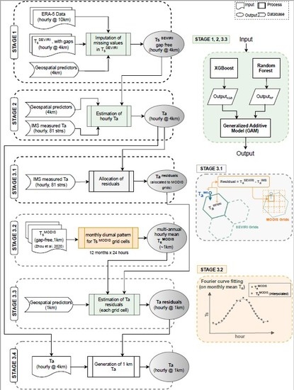
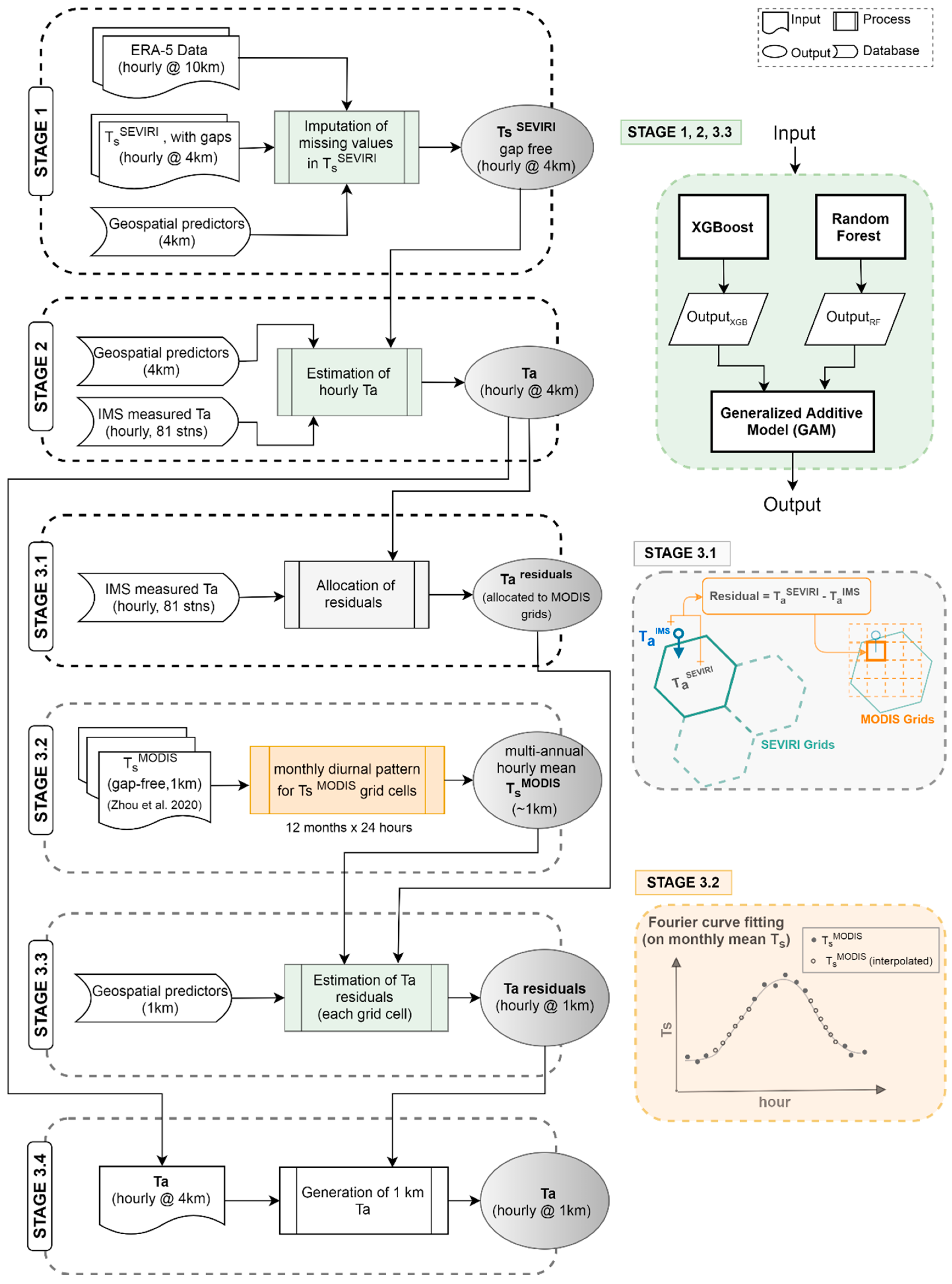
2.5. Statistical Methods

We propose a three-stage ensemble model approach based on established machine learning algorithms—Random Forest (RF) [37] and Extreme Gradient Boosting (XGBoost) [38]—to estimate the near-surface air temperature (Ta) from the surface skin temperature (Ts), as shown in Figure 2.

RF and XGBoost are both decision tree-based learning methods where multiple decision trees are built using a randomly selected subset of data for each tree (bagging) to achieve an ensemble prediction. As RF builds trees independent of each other in a parallel and distributed fashion, the construction of a RF model for large datasets consisting of hundreds of trees can become time- and memory-intensive. In contrast, the sequential trees building together with other systems and algorithmic optimizations implemented in XGBoost make XGBoost extremely memory- and computation-efficient [38].

A common rule of thumb for any data-driven machine learning-based model is to incorporate as much data as possible provided data are properly collected with reasonable acquisition cost [39]; this would imply that it is optimal to train models using the entire data considered in this study. However, due to the limitation of available memory and volume of data considered in each stage, we ran RF and XGBoost using data of different lengths of time in different stages.

Once predictions from RF and XGBoost had been obtained in each stage, an additional geographically weighted GAM was employed to leverage the predicting power of each model in different regions.

In the first stage we imputed satellite-based SEVIRI Ts values for missing Ts grid cells (obscured by cloud cover, etc.). Then we fed the imputed SEVIRI Ts for each grid cell into the Stage 2 model to predict hourly Ta at 4 × 4 km². In Stage 3, residuals of the predicted Ta, i.e., difference between predicted and measured Ta (at a weather station located within the 4 × 4 km² SEVIRI grid cell), were allocated to the MODIS 1 × 1 km² gridding system (see Figure 2, Stage 3.1). We estimated Ta residuals across the entire country by taking into account the monthly mean diurnal pattern of Ts derived from the multi-annual MODIS observations from 2004–2017. By re-adding Ta residuals estimated hourly at 1 × 1 km² to the 4 × 4 km² Ta from Stage 2, we obtained the hourly Ta estimation at 1 × 1 km².

We performed the machine learning algorithms using the R mlr package [40], which wraps the ranger package [41] for RF, and the xgboost package [42] for XGBoost. The GAM model was run using the mgcv package [26].

2.5.1. Stage 1 Model: Imputation of SEVIRI Ts

The Stage 1 model aims at imputing hourly SEVIRI Ts over the entire study area across the investigating period to account for missing data due to cloud cover. For both RF and XGBoost models, we fed the model with the same set of predictor variables, i.e., hour, day of the year (DoY), spatial coordinates (longitude and latitude), and selected synoptic variables from the ERA5 reanalysis data described in Section 2.3, as well as the geospatial variables in Section 2.4. The target variable is the clear-sky Ts observed by SEVIRI. Once trained, the two models were applied to impute Ts for the entire study area, respectively. Due to the large data volume, we ran the RF and XGBoost models for each month individually. The imputed gap-free Ts are subsequently put into a geographically weighted GAM ensemble model to generate a harmonized estimate of Ts (see Equation (1)):

$$\mathrm{GAM}{\left({\mathrm{T}}_{\mathrm{S}}\right)}_{\mathrm{i},\mathrm{t}} ~ \mathrm{t}\mathrm{e}{\left(\mathrm{X},\mathrm{Y},\mathrm{b}\mathrm{y}={\mathrm{T}}_{\mathrm{S}}^{\mathrm{R}\mathrm{F}}\right)}_{\mathrm{i},\mathrm{t} }+ \mathrm{t}\mathrm{e}{\left(\mathrm{X},\mathrm{Y},\mathrm{b}\mathrm{y}={\mathrm{T}}_{\mathrm{S}}^{\mathrm{X}\mathrm{G}\mathrm{B}\mathrm{o}\mathrm{o}\mathrm{s}\mathrm{t}}\right)}_{\mathrm{i},\mathrm{t} }+{\mathsf{\epsilon }}_{\mathrm{i},\mathrm{t}}$$

(1)

where ${\mathrm{T}}_{\mathrm{s}}{}_{\mathrm{i},\mathrm{t}}$ is the observed SEVIRI Ts of grid cell $\mathrm{i}$ at time $\mathrm{t}$; $\mathrm{te}$ are 2-dimensional tensor product smooths of projected X- and Y-coordinates; and ${\mathsf{ϵ}}_{\mathrm{i},\mathrm{t}}$ is the error term. $\mathrm{te}$ gets multiplied by ${\mathrm{T}}_{\mathrm{s}}^{\mathrm{RF}}$ and ${\mathrm{T}}_{\mathrm{s}}^{\mathrm{X}\mathrm{G}\mathrm{B}\mathrm{o}\mathrm{o}\mathrm{s}\mathrm{t}}$—Ts estimated from RF and XGBoost, respectively—to account for the contribution of each model to the final Ts estimation, which is a function of space and time.

2.5.2. Stage 2 Model: Imputation of Ta from Ts

The Stage 2 model seeks to obtain a gridded, gap-free, hourly estimate of Ta based on the Ts obtained from the previous stage. We took the hourly observed Ta from the IMS stations as the ground-truth target variable. Each IMS station was assigned to a SEVIRI grid cell that encompasses the station. Where more than one weather station is located within the same SEVIRI grid cell, values from all stations were first averaged and then used for further steps. Similarly, to the Stage 1 model, we first trained the RF and XGBoost models based on data from grid cells with ground-truth measurement. Once calibrated and validated, the trained model is applied to impute Ta for all grid cells, including those without ground-truth measurement.

The Stage 2 model incorporated the following predictor variables: hour, day of year (DoY), month, and spatial coordinates (x- and y-coordinates), as well as the geospatial variables described in Section 2.4. Once obtained, the imputed Ta from the RF and the XGBoost for the period of investigation (2004–2017) are incorporated into GAM to further enhance the accuracy of the modeled Ta. In this stage, the RF, XGBoost, and GAM models are run for each year individually.

2.5.3. Stage 3 Model: Downscaling to 1 km Ta by Estimating Residuals

The Stage 3 model aims to further downscale Ta to 1 × 1 km² spatial resolution by accounting for the variability of Ta within each SEVIRI cell. We first allocated the residuals of Ta, i.e., the difference between Ta estimated from Stage 2 and observed Ta from IMS weather stations, to individual MODIS cells at 1 × 1 km², based on the geographical location of IMS weather stations (Stage 3.1 in Figure 2).

In addition to the predicting variables in the Stage 2 model, we incorporated the monthly mean diurnal patterns of Ts, averaged over 2004–2017 for each MODIS cell, to account for Ta variation among cells. The derivation of the diurnal pattern was based on the MODIS Ts dataset described in Section 2.2. Applying a first-order Fourier curve fitting technique to the monthly mean hourly Ts, we retrieved the monthly mean diurnal pattern of Ts (Stage 3.2 in Figure 2).

RF and XGBoost models were trained and then applied to estimate the residuals of Ta. An ensemble GAM was again invoked in this stage to fine-tune the estimated Ta residuals from both learners across all years. We subtracted the 1 × 1 km² residuals from the 4 × 4 km² Ta estimates obtained in Stage 2 to produce the final hourly Ta at 1 × 1 km².

2.5.4. Tuning of Hyper Parameters and Evaluation of Model Performance

Machine learning algorithms normally demand optimization of hyper-parameters that control the learning process. A carefully optimized model yields robust outputs while minimizing the risk of overfitting. We applied the tuneRanger package [43] and the autoxgboost package [44] to tune the RF and XGBoost models, respectively.

For RF, we tuned the following hyper-parameters: (1) mtry (number of variables available for splitting at each tree node), (2) min.node.size (minimum number of observations in a terminal node), and (3) sample.fraction (fraction of observations available for splitting at each tree node). The number of trees is set at 300.

For XGBoost, we tuned four hyper-parameters: (1) eta, (2) alpha, (3) gamma, and (4) max_depth. In contrast to RF, where trees are independent, XGBoost originates from the gradient boosting decision tree algorithm [38] where new trees are created stepwise to predict residuals or errors of previous trees and then added together to make a final prediction. Therefore, to avoid over-fitting, it incorporates several hyperparameters to account for the learning rate (e.g., eta, gamma, max_depth) and for the regularization (alpha). The results of hyper-parameters tuned in the models of each stage can be found in detail in Tables S2–S5 in the SI.

To evaluate the model performance, we applied the out-of-sample 5-fold cross-validation (CV) (see Figure 3). The observations (predictor features + target variable) fed into the model were partitioned into five random subsets of equal size. Each subset was iteratively used for testing model performance, while the remaining four sub-sets comprised the training set. Mean absolute error (MAE), root mean square error (RMSE), and the coefficient of determination (R²) were calculated between the cross-validated target variable and the ground-truth target variable (Ts in Stage 1, Ta in Stage 2, and residuals of Ta in Stage 3). Meanwhile, we disaggregated the overall performance into spatial and temporal components to assess the model’s capacity to capture the spatio-temporal variability, as employed in [15,45].

3. Results

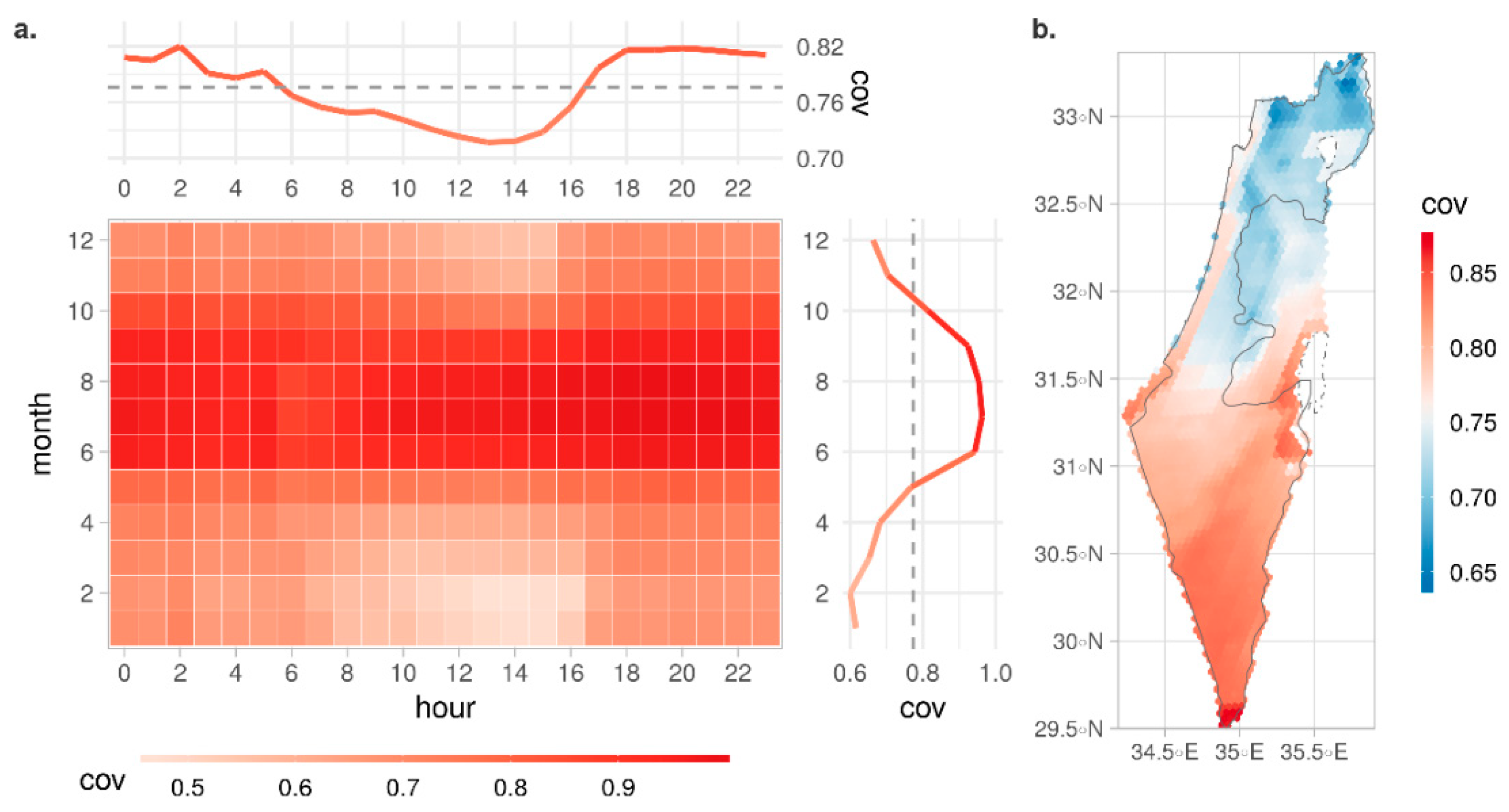
3.1. SEVIRI Data Coverage

The Stage 1 model involves the process of imputing missing values of SEVIRI Ts. As the distribution of missing values could affect the quality of estimation [25], we checked the spatio-temporal pattern of the clear-sky ratio for the multi-annual SEVIRI Ts data from 2004–2017 across Israel, as shown in Figure 4a,b. The monthly variation of the clear-sky ratio is highly consistent with the pattern of precipitation in Israel: The clear-sky ratio remains high (above 80%) in the dry season from June to September, whereas it reaches its minimum value in December through February, when rainfall peaks [32]. With respect to the diurnal pattern, the clear-sky ratio declines from the early morning to afternoon, which coincides with the primary afternoon peak of the convective rainfall, and with the early morning secondary peak in the Mediterranean region [46,47].

3.2. Performance of the Stage 1 Model

3.2.1. Feature Importance of RF and XGBoost Models in Stage 1

Figure 5 shows the relative impurity-based importance of individual features in RF and XGBoost in Stage 1 and the ranking changes between the two models. Feature importance indicates how each feature contributes to outcomes estimation [37]. Features that better account for the variance of the target variable at each tree node split (weighted by the number of samples reaching the node) are given higher values of importance. As the ranking drops, the feature importance decreases exponentially. In both RF and XGBoost, surface skin temperature (skt) and 2 m air temperature (2t) from the ERA5 reanalysis data take on the highest relevance in estimating the SEVIRI Ts. In contrast, temporally invariant features, for example, population and road densities, exhibit low importance in both models.

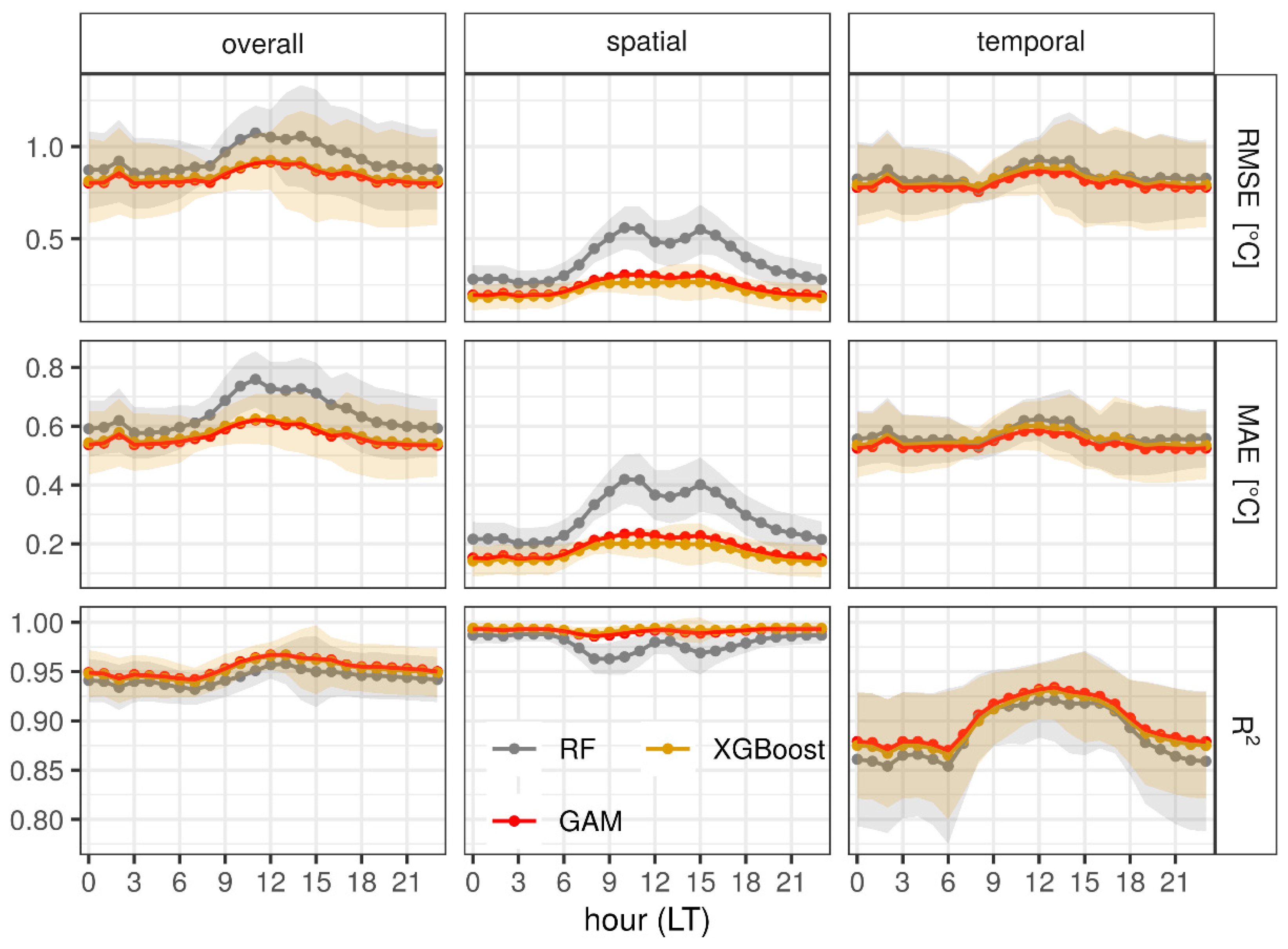
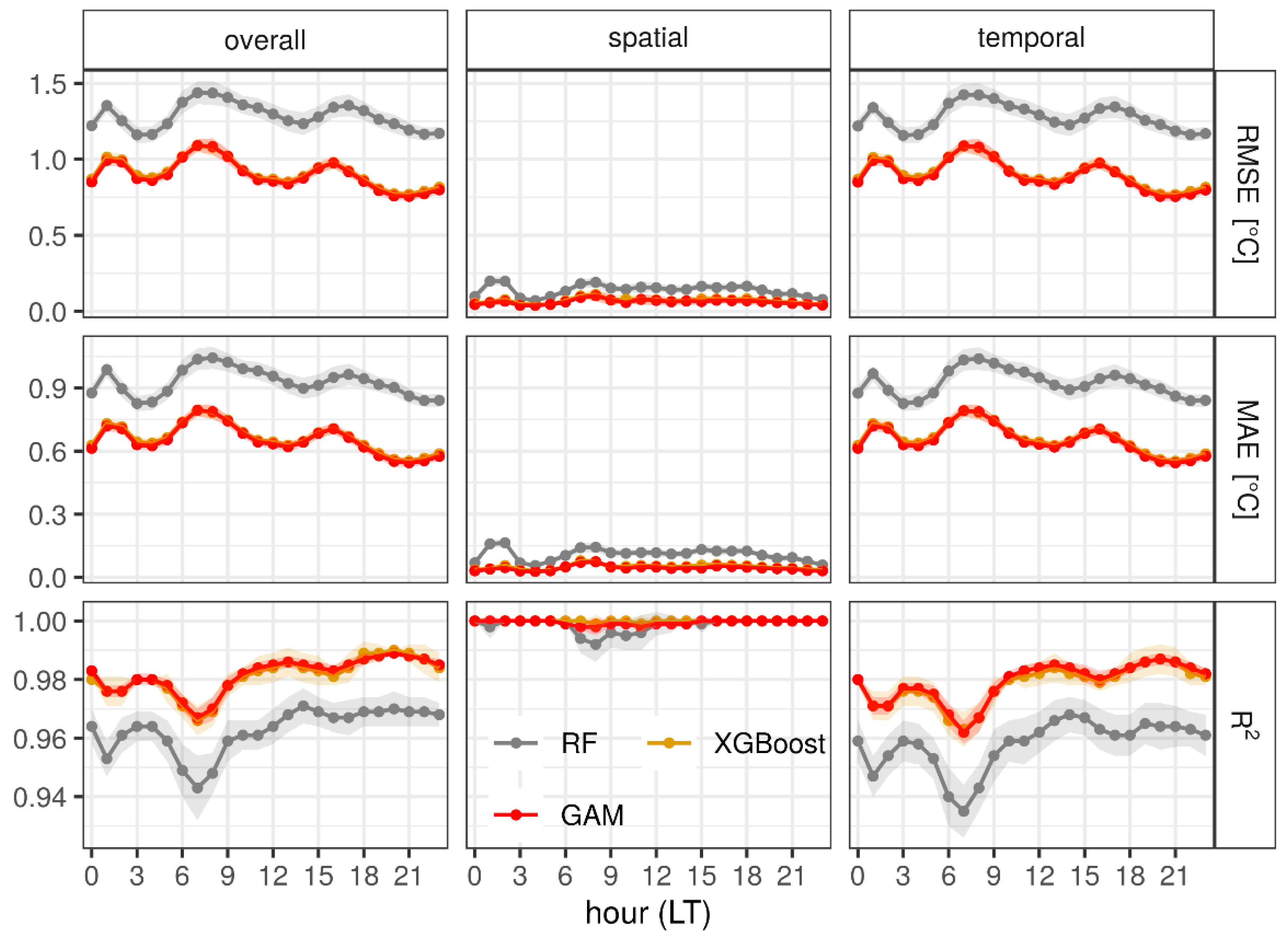
3.2.2. Overall, Temporal, and Spatial Performance

Figure 6 shows the mean performance (RMSE, MAE, R²) of individual models in Stage 1 based on the 5-fold CV performed for each year. It is apparent that XGBoost outperforms RF by all measures, whereas GAM presents an additional performance increase over XGBoost. In overall terms, the ensemble GAM model attains a cross-validated RMSE of about 0.8 °C, MAE of less than 0.6 °C and R² of 0.95. The two methods differ in their ability to address the diurnal variability: the performance of RF exhibits a pronounced variability with the time of day, with relatively lower performance around noon, whereas such variability vanishes in XGBoost and GAM.

In terms of the models’ capacity to account for the spatial variance of Ts, RF demonstrates a modest performance during the daytime, which is ascribed primarily to the performance drop in the transitional seasons (spring from March–April, and autumn from October–November). See Figures S1–S3 in the SI for more details. In the transitional seasons, especially spring, an oppressive, southeasterly hot wind blowing from North Africa, termed “hamsin” (fifty in Arabic), can typically last a few days, resulting in high atmospheric turbidity caused by sand and dust storms, and a drastic temperature increase (sometimes more than 10 °C) within a day [32]. After the events, temperatures fall rapidly back to pre-event values, causing considerable fluctuations and deviations in temperatures during the transitional seasons. This affects particularly the RF algorithm, where the construction of trees is independent, i.e., some trees are more adaptive to the dynamic training data while some fail. In contrast, trees are built sequentially in XGBoost—each tree learns from the previous ones, which makes XGBoost more robust to the variation of data and therefore improves the ensemble performance.

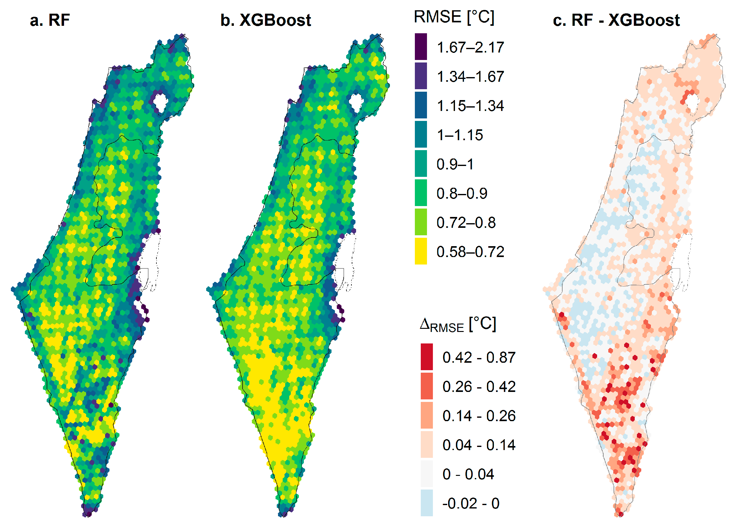
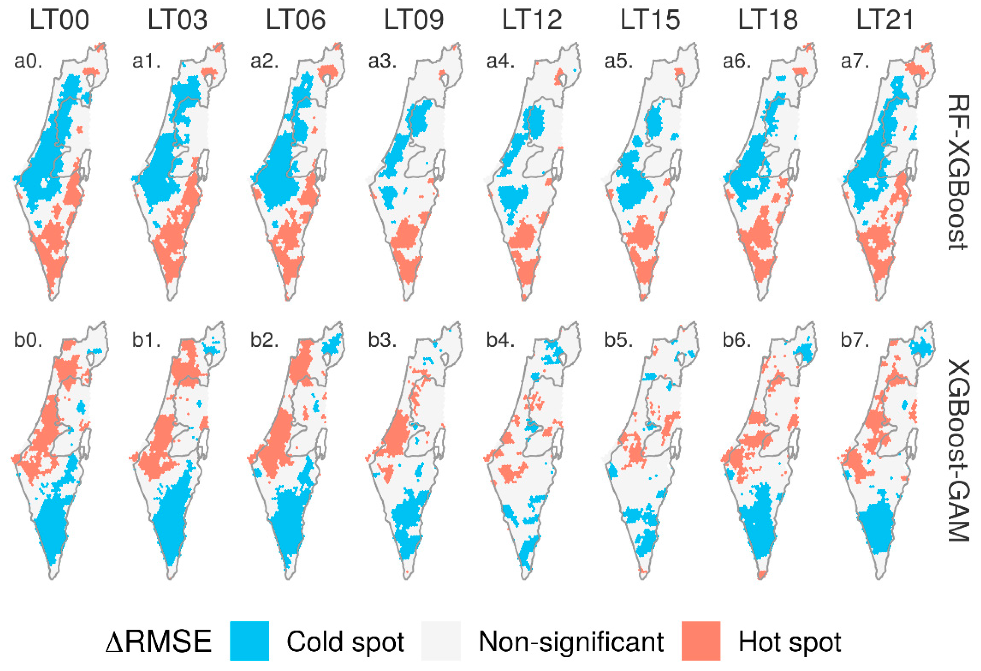
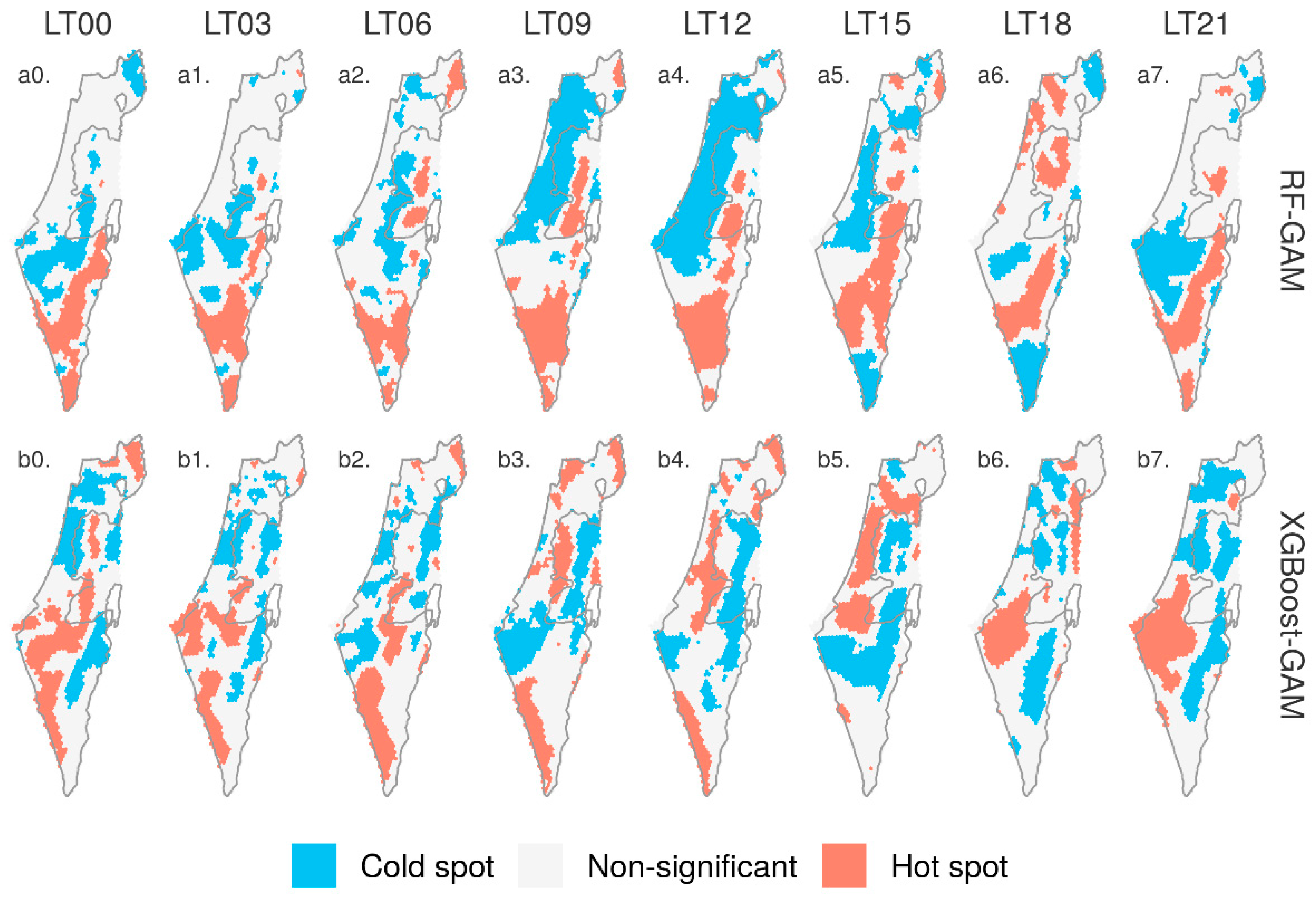
3.2.3. Spatial Pattern of Performance

Figure 7 shows the spatial pattern of multi-annual overall RMSE from RF and XGBoost, as well as the difference between them. Three distinctive features can be observed: (1) In both models, grid cells in proximity to bodies of water are less predictable than those in inland areas; (2) RF exhibits a sharp transition in performance between adjacent grid cells, particularly in southern Israel, whereas this is absent in XGBoost; (3) XGBoost outperforms RF mainly in the semi-arid South, Jordan Rift Valley, and the Golan Heights in the North, while in other parts the difference is negligible. Analyses based on MAE and R² show consistent results (see Figures S4 and S5 in the SI).

To analyze spatial clustering of performance, we performed a hot/cold spot analysis by calculating the Getis-Ord Gi* statistic using the spdep package [48]. The Gi* statistic returned a z-score of each grid cell taking into account its 5 × 5 neighborhood: high positive (>1.96) and negative (<−1.96) values indicate significantly hot and cold spots at a confidence interval of 95%, respectively [49,50].

Figure 8 shows the spatio-temporal patterns of the performance difference between pairs of models at three-hour intervals. As GAM approximates XGBoost in model performance, the differences between RF and GAM resemble those between RF and XGBoost, and thus are not shown here. RF outperformed XGBoost in the central plains during the nighttime, while the performance superiority diminishes notably during the daytime (a0–a7). In contrast, XGBoost performs better in the Negev desert of southern Israel and the region north of the Sea of Galilee. Since GAM synergizes the estimates from both models by incorporating spatial smoothing, it achieves an optimal compromise between the two models: GAM outperforms RF in southern Israel, and XGBoost in central Israel, respectively (b0–b7).

3.2.4. Spatial Pattern of Imputed Ts of the Stage 1 Model

Figure 9 shows the spatio-temporal pattern of multi-annual mean hourly SEVIRI Ts at 2-h intervals, imputed by GAM in Stage 1. The pattern is generally consistent with the long-established climatological records of Ta: (1) Ts decreases northward and with higher altitude, the latter of which accounts for the hot and cold spots in the Jordan Rift Valley (especially around the Dead Sea and Arava Valley) and Golan Heights, respectively; and (2) extremes of Ts increase with distance from the Mediterranean [32].

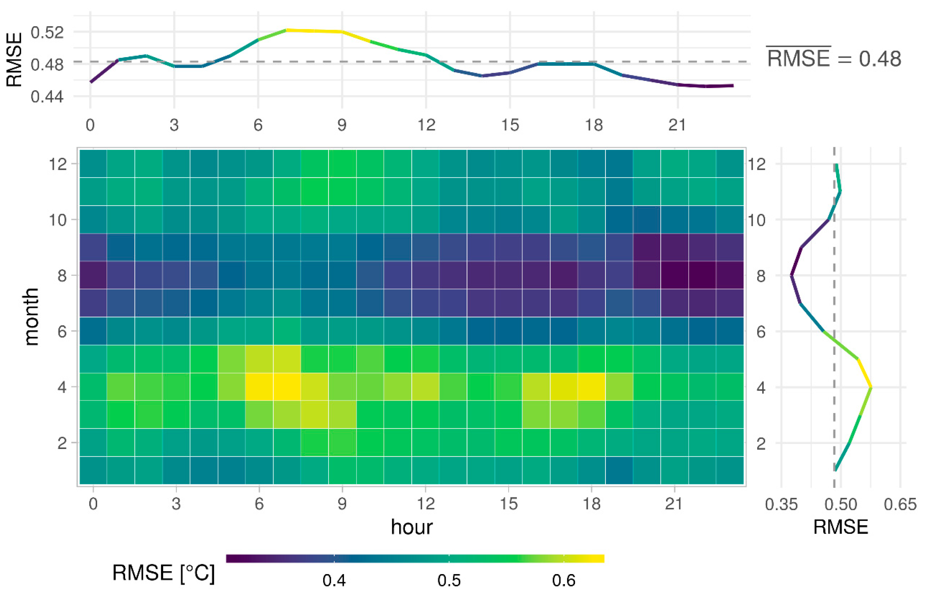
3.3. Performance of the Stage 2 Model

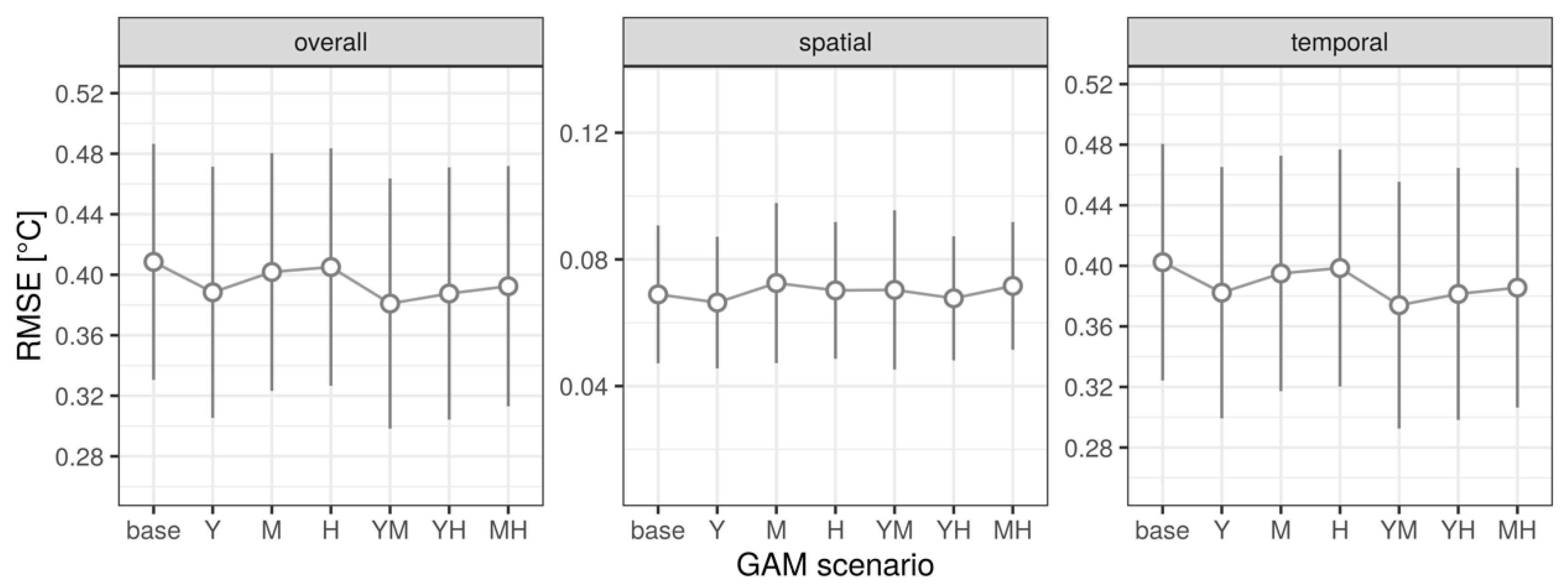
3.3.1. Feature Importance and Model Performance in Stage 2

Like in Stage 1, surface skin temperature (Ts), elevation, and predictor features that indicate time (hour, DoY), are ranked high in both models (see Figure S6 in the SI). This highlights the importance of Ts and topography in accounting for the spatial variability of near-surface air temperature [19,51]. In contrast, the socio-economic variables, such as population and road densities, are consistently ranked low.

Figure 10 shows the performance of each model in Stage 2. Although XGBoost and RF exhibit similar diurnal variation in performance, XGBoost significantly outperforms RF in all indicators.

In line with the results from Stage 1, the Stage 2 ensemble GAM model enhances the performance beyond both individual base models—namely RF and XGBoost—and slightly outperforms the superior XGBoost model. The Stage 2 GAM model inherits the better accountability of XGBoost for the temporal variance of Ta, as shown in the third column of Figure 10. Overall, GAM achieves an RMSE of about 0.9 °C, MAE of 0.7 °C and R² of 0.98.

Compared to Stage 1, where GAM is applied to Ts data on a regular grid, the data incorporated into Stage 2 are composed of Ta observations from the sparsely scattered IMS weather stations, which enables a higher degree of freedom in smoothing splines. The variation of GAM performance across weather stations is illustrated in Figure S7 in the SI. The performance differs slightly across stations and does not exhibit pronounced spatial patterns, which is generally an indication of unbiased estimation of GAM over space.

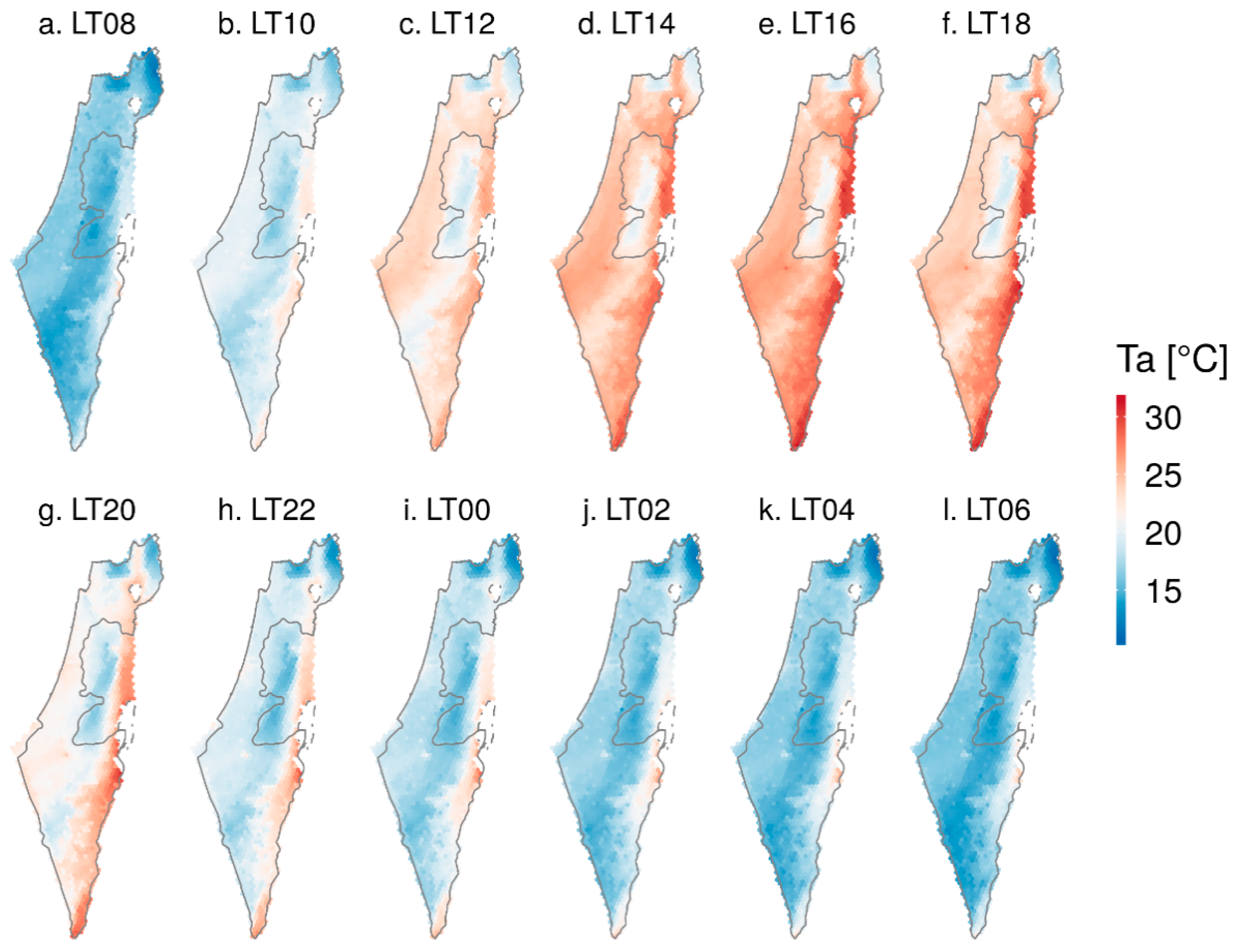
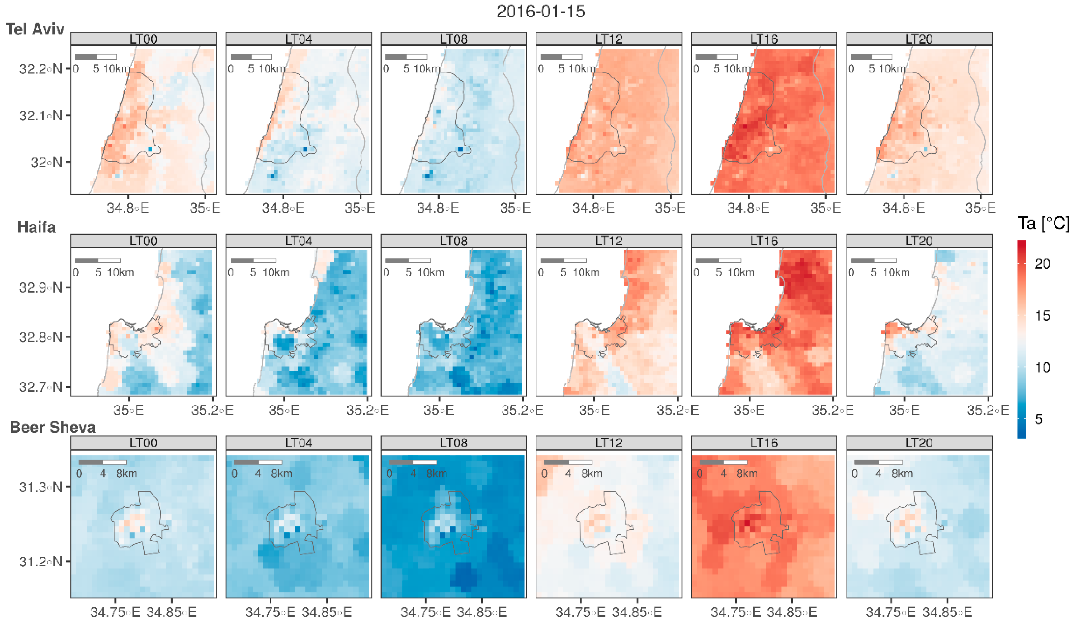
3.3.2. Spatio-Temporal Pattern of Ta Estimated from the Stage 2 Models

Figure 11 depicts the spatio-temporal hot/cold clusters using Gi* statistics based on the difference in estimated multi-annual mean Ta between RF and GAM (a0–a7), and between XGBoost and GAM (b0–b7). The pattern of clustering visualizes how GAM spatio-temporally smooths the estimates of RF and XGBoost to achieve better ensemble estimation of Ta (as demonstrated in Figure 10): GAM adjusts the RF estimates downwards in most parts of southern Israel, while increasing its estimates in the coastal plain during the daytime. Meanwhile, GAM lowers nighttime Ta estimates by XGBoost in the Negev dune field near the Gaza strip and the hilly southern part of the Negev on the border to the Egyptian border. Finally, GAM adjusts the daytime Ta estimate by XGBoost upwards in the Negev dune field, as well as the in the Judaean Mountains in central Israel. However, Figure 11 and the underlying analysis indicate by no means that GAM better estimates Ta over RF and XGBoost ubiquitously in absolute terms; they rather aim to investigate the origin and reason why GAM outperforms RF and XGBoost.

Figure 12 shows the multi-annual (2004–2017) mean Ta estimated by GAM at 2-h intervals. The estimates range from 11.3 to 31.3 °C with a notable diurnal variation. The daytime and nighttime mean Ta are 21.8 and 18.6 °C, respectively. The Jordan Rift Valley constitutes the hot spot throughout the day because of its low elevation (as low as 430 m below sea level), which is consistent with the spatial pattern of Ts in Stage 1.

We further scrutinized the model’s performance when estimating Ta at certain daytime/nighttime hours of a summer/winter day, in order to illustrate the model’s accountability for short-term variability, rather than merely for long-term means. Figure 13 presents an example for the input data and the outputs achieved for the first two modeling stages for two specific hours (nighttime (LT 0100, a–f) and daytime (LT 1500, g–l)) on a selected summer day. To highlight the model’s capacity to impute missing values, we chose a day with relatively high cloud cover. The Ts and Ta estimated by the ensemble model from both stages do not show any artifacts and clumping, which indicates a sound performance of the model and complements the quantitative cross-validation assessment. Similar results for a winter day are presented in Figure 14, again exhibiting satisfactory performance.

3.4. Performance of the Stage 3 Model

Figure 15 and Figure 16 present the 5-fold cross-validated RMSE and R² of the ensemble GAM model in Stage 3, respectively. As the figures show, the model also performs well in estimating the hourly residuals of Ta, with overall RMSE of 0.48 °C and R² of 0.63. However, the figures also illustrate clear diurnal and seasonal variation: the best performance appears in the nighttime during hot summer months (June–September), whereas the model performs below average in the transitional season (March and April), and around the noon in the winter months (December and January).

Figure 17 shows the spatial pattern of estimated hourly Ta at 1 × 1 km² at 4 h intervals for three metropolitan areas in Israel—Tel Aviv (central), Haifa (north), and Beer Sheva (south)—on a typical summer day of 11 August 2010. In all three cities, the urban heat island effect is clearly observed, where the urban area is several degrees warmer relative to its natural surroundings. As Tel Aviv and Haifa are located along the Mediterranean coast, the sea breeze from the west during the day could to some extent mitigate the heat flux stored and trapped in the city through convective cooling, resulting even in a slightly increased temperature gradient landwards, as shown in Tel Aviv at LT 16:00. In contrast, Beer Sheva, located in the Negev desert of southern Israel, exhibits a more pronounced urban heat island during the night, because its barren rural area devoid of vegetation cools more rapidly than urban surfaces of higher thermal mass [52]. Similarly, Figure 18 shows the spatial pattern of estimated Ta for a typical winter day of 15 January 2016.

4. Discussion

The paper presents a three-stage GAM-based ensemble model to estimate hourly near-surface air temperature (Ta) at a high spatial resolution of 1 × 1 km² across Israel from 2004–2017. The model demonstrates an overall satisfactory performance in imputing Ts and estimating Ta, while accounting adequately for their spatial and temporal variation. Compared to models based exclusively on a single method, the ensemble model can improve the results of its constituent models, which is consistent with previous GAM-based studies [28,30].

Despite the overall satisfactory performance of our model, we acknowledge several limitations of the study.

First, the model can only achieve a high temporal resolution by adopting hourly Ts from the geostationary SEVIRI satellite, which has a low spatial resolution. Consequently, grid cells in coastal areas may be classified as bodies of water, despite having substantial land areas. In particular, this affects densely populated urban coastal areas, such as Tel Aviv and Haifa, where the waterfront is quite populous. To minimize the gaps in these regions which comprise a substantial proportion of the population, the Stage 1 model does (exceptionally) impute Ts for the coastal SEVIRI grid cells within dense metropolitan areas. Those cells (involving a total number of 4–5) were manually fed into the trained model to obtain land-like Ts, although they are labeled “water” in the SEVIRI water mask product.

Second, in RF and XGBoost, static socio-economic variables (e.g., road and population densities, urban fraction) which vary in space but not in time, are ranked lowest in terms of feature importance. However, the adoption of these variables is mostly ascribed to their relevance to temperature variability through anthropogenic activities, especially over artificial surfaces, such as residential and industrial areas in cities [10,53]. In general, tree-based algorithms are regarded as insensitive to overfitting [37], and the inclusion of static variables into models may result in a decrease in model performance [54]. However, as shown in the outcomes, XGBoost markedly outperforms RF, implying that the sequential tree-growing in XGBoost may help to gradually filter out the lowly rated static variables to achieve better performance. On the other hand, time series of non-static variables, e.g., temperatures and NDVI, encompass, to some extent, the biophysical information inherent in the static variables, which can also be learned by the model automatically. Therefore, further study is required as to what extent a thorough elimination of static variables in machine learning-based models affects the model performance.

Third, it is widely found through observations and numerical simulation that cities in arid/semi-arid and Mediterranean climate zones, such as Beer Sheva in Israel, sometimes develop a daytime urban oasis effect in terms of both Ts and Ta: i.e., the urban area is cooler relative to the rural hinterland [52,55,56,57]. This could be ascribed both to the regional natural land cover where a city resides, and to the cooling effect resulting from the irrigation of urban green spaces. The surface energy balance above sparsely vegetated shrub land and desert commonly found outside of Israeli cities typically display a larger Bowen ratio, which favors the partitioning of energy flux to sensible heat and thus results in greater heating rates of rural areas when exposed to solar radiation.

However, the oasis effect is mostly absent in our results, which we attribute to the differences in how physically based models and statistical models address energy balance and anthropogenic heat. In numerical models, the complex urban landscape is normally simplified using parameters such as aspect ratio of street canyon and albedo, to account for the energy budget of an urban canopy layer. In contrast, statistical models like the ones used in this study are based on a set of common rules derived from the data incorporated. In terms of the predicting variables included in the model to account for urban-specific features, it is assumed that grid cells with similar population density, road density, and urban fraction, should behave alike in terms of the temperature dynamics. However, to what extent the rules hold true depends not only on the model’s capability and sensitivity in discerning the nuances inherent in the data. The quantity of data could also influence the results. For any data-driven approach, the rule of thumb seems to be that “the more, the better”. In this sense, an increase of urban monitoring stations incorporated into the model, which are currently unevenly distributed and are extremely sparse in southern Israel (see Figure 1), may promise better Ta estimation.

In this study, we ran an ensemble model (GAM) based on input data (results from RF and XGBoost) across an extended period of investigation (the base scenario). To check whether the scenario specified for running GAM affects the estimation performance, we conducted an uncertainty analysis in the Stage 2 model through applying GAM to data partitioned by different scenarios. At Y (year), M (month), H (hour) scenarios, GAM is applied on data of each year, data of same month across all years, and same hour across all years, respectively. At YM (year-month), YH (year-hour), and MH (month-hour) scenarios, data are partitioned jointly by “year and month”, “year and hour”, and “month and hour”, respectively. As shown in Figure 19, the difference in RMSE between scenarios is non-significant, indicating that GAM is insensitive to the scenario of running it and is therefore robust when applied to spatio-temporal data over long periods.

5. Conclusions

In conclusion, the ensemble model proposed in this study realized a seamless mapping of hourly resolved Ta at a high spatial resolution of 1 × 1 km². This study achieves the aim to predict Ta at a high spatio-temporal resolution while simultaneously attaining a satisfactory performance. The Ta data produced in this study underlie effective monitoring and assessment of human health exposure to temperature extremes first on a regional scale, yet with a scale-up potential to a wider geographical area. Since the physical processes determining the temperature variability are accounted for in a modest manner, the machine learning-based model achieves a balanced complexity, computational efficiency, and ease of use. The performance enhancement promised by the ensemble GAM model helps to further minimize exposure misclassification in epidemiological studies.

In future work, the outcomes of this study may subsequently be integrated into modeling schemes, such as image fusion and spatial sharpening [58], to improve the spatial resolution of Ta.

References

1. Johnson, N.C.; Xie, S.P.; Kosaka, Y.; Li, X. Increasing occurrence of cold and warm extremes during the recent global warming slowdown. Nat. Commun. 2018, 9, 4–6. [Google Scholar] [CrossRef] [Green Version]
2. Horton, D.E.; Johnson, N.C.; Singh, D.; Swain, D.L.; Rajaratnam, B.; Diffenbaugh, N.S. Contribution of changes in atmospheric circulation patterns to extreme temperature trends. Nature 2015, 522, 465–469. [Google Scholar] [CrossRef] [Green Version]
3. Coumou, D.; Robinson, A. Historic and future increase in the global land area affected by monthly heat extremes. Environ. Res. Lett. 2013, 8, 034018. [Google Scholar] [CrossRef]
4. Rahmstorf, S.; Coumou, D. Increase of extreme events in a warming world. Proc. Natl. Acad. Sci. USA 2011, 108, 17905–17909. [Google Scholar] [CrossRef] [Green Version]
5. Gasparrini, A.; Guo, Y.; Hashizume, M.; Lavigne, E.; Zanobetti, A.; Schwartz, J.; Tobias, A.; Tong, S.; Rocklöv, J.; Forsberg, B.; et al. Mortality risk attributable to high and low ambient temperature: A multicountry observational study. Lancet 2015, 386, 369–375. [Google Scholar] [CrossRef]
6. Wang, Y.; Shi, L.; Zanobetti, A.; Schwartz, J.D. Estimating and projecting the effect of cold waves on mortality in 209 US cities. Environ. Int. 2016, 94, 141–149. [Google Scholar] [CrossRef] [Green Version]
7. Huang, C.; Barnett, A.G.; Wang, X.; Vaneckova, P.; FitzGerald, G.; Tong, S. Projecting Future Heat-Related Mortality under Climate Change Scenarios: A Systematic Review. Environ. Health Perspect. 2011, 119, 1681–1690. [Google Scholar] [CrossRef] [Green Version]
8. Kloog, I.; Melly, S.J.; Coull, B.A.; Nordio, F.; Schwartz, J.D. Using satellite-based spatiotemporal resolved air temperature exposure to study the association between ambient air temperature and birth outcomes in Massachusetts. Environ. Health Perspect. 2015, 123, 1053–1058. [Google Scholar] [CrossRef] [Green Version]
9. Arnfield, A.J. Two decades of urban climate research: A review of turbulence, exchanges of energy and water, and the urban heat island. Int. J. Climatol. 2003, 23, 1–26. [Google Scholar] [CrossRef]
10. Oke, T.R.; Mills, G.; Christen, A.; Voogt, J.A. Urban Climates; Cambridge University Press: Cambridge, UK, 2017; ISBN 9781139016476. [Google Scholar]
11. Erell, E.; Pearlmutter, D.; Williamson, T. Urban Microclimate: Designing the Spaces between Buildings; Earthscan: London, UK, 2011. [Google Scholar]
12. Zeger, S.L.; Thomas, D.; Dominici, F.; Samet, J.M.; Schwartz, J.; Dockery, D.; Cohen, A. Exposure measurement error in time-series studies of air pollution: Concepts and consequences. Environ. Health Perspect. 2000, 108, 419–426. [Google Scholar] [CrossRef]
13. Mirzaei, P.A.; Haghighat, F. Approaches to study Urban Heat Island—Abilities and limitations. Build. Environ. 2010, 45, 2192–2201. [Google Scholar] [CrossRef]
14. Rosenfeld, A.; Dorman, M.; Schwartz, J.; Novack, V.; Just, A.C.; Kloog, I. Estimating daily minimum, maximum, and mean near surface air temperature using hybrid satellite models across Israel. Environ. Res. 2017, 159, 297–312. [Google Scholar] [CrossRef]
15. Kloog, I.; Nordio, F.; Lepeule, J.; Padoan, A.; Lee, M.; Auffray, A.; Schwartz, J. Modelling spatio-temporally resolved air temperature across the complex geo-climate area of France using satellite-derived land surface temperature data. Int. J. Climatol. 2017, 37, 296–304. [Google Scholar] [CrossRef]
16. Janatian, N.; Sadeghi, M.; Sanaeinejad, S.H.; Bakhshian, E.; Farid, A.; Hasheminia, S.M.; Ghazanfari, S. A statistical framework for estimating air temperature using MODIS land surface temperature data. Int. J. Climatol. 2017, 37, 1181–1194. [Google Scholar] [CrossRef]
17. Kloog, I.; Chudnovsky, A.; Koutrakis, P.; Schwartz, J. Temporal and spatial assessments of minimum air temperature using satellite surface temperature measurements in Massachusetts, USA. Sci. Total Environ. 2012, 432, 85–92. [Google Scholar] [CrossRef] [Green Version]
18. Kilibarda, M.; Hengl, T.; Heuvelink, G.B.M.; Gräler, B.; Pebesma, E.; Perčec Tadić, M.; Bajat, B. Spatio-temporal interpolation of daily temperatures for global land areas at 1 km resolution. J. Geophys. Res. Atmos. 2014, 119, 2294–2313. [Google Scholar] [CrossRef] [Green Version]
19. Oyler, J.W.; Ballantyne, A.; Jencso, K.; Sweet, M.; Running, S.W. Creating a topoclimatic daily air temperature dataset for the conterminous United States using homogenized station data and remotely sensed land skin temperature. Int. J. Climatol. 2015, 35, 2258–2279. [Google Scholar] [CrossRef]
20. Meyer, H.; Katurji, M.; Appelhans, T.; Müller, M.U.; Nauss, T.; Roudier, P.; Zawar-Reza, P. Mapping daily air temperature for Antarctica Based on MODIS LST. Remote Sens. 2016, 8, 732. [Google Scholar] [CrossRef] [Green Version]
21. Li, L.; Zha, Y. Mapping relative humidity, average and extreme temperature in hot summer over China. Sci. Total Environ. 2018, 615, 875–881. [Google Scholar] [CrossRef]
22. Hough, I.; Just, A.C.; Zhou, B.; Dorman, M.; Lepeule, J.; Kloog, I. A multi-resolution air temperature model for France from MODIS and Landsat thermal data. Environ. Res. 2020, 183, 109244. [Google Scholar] [CrossRef]
23. Prigent, C.; Aires, F.; Rossow, W.B. Land surface skin temperatures from a combined analysis of microwave and infrared satellite observations for an all-weather evaluation of the differences between air and skin temperatures. J. Geophys. Res. 2003, 108, 1–14. [Google Scholar] [CrossRef]
24. Prihodko, L.; Goward, S.S.N. Estimation of air temperature from remotely sensed surface observations. Remote Sens. Environ. 1997, 4257, 335–346. [Google Scholar] [CrossRef]
25. Zhou, B.; Erell, E.; Hough, I.; Rosenblatt, J.; Just, A.C.; Novack, V.; Kloog, I. Estimating near-surface air temperature across Israel using a machine learning based hybrid approach. Int. J. Climatol. 2020. [Google Scholar] [CrossRef] [Green Version]
26. Wood, S.N. Generalized Additive Models, 2nd ed.; Chapman and Hall/CRC: London, UK, 2017; ISBN 9781315370279. [Google Scholar]
27. Hastie, T.; Tibshirani, R. Generalized Additive Models. In Wiley StatsRef: Statistics Reference Online; John Wiley & Sons, Ltd.: Chichester, UK, 2014. [Google Scholar]
28. Di, Q.; Amini, H.; Shi, L.; Kloog, I.; Silvern, R.; Kelly, J.; Sabath, M.B.; Choirat, C.; Koutrakis, P.; Lyapustin, A.; et al. An ensemble-based model of PM2.5 concentration across the contiguous United States with high spatiotemporal resolution. Environ. Int. 2019, 130, 104909. [Google Scholar] [CrossRef]
29. Ravindra, K.; Rattan, P.; Mor, S.; Aggarwal, A.N. Generalized additive models: Building evidence of air pollution, climate change and human health. Environ. Int. 2019, 132, 104987. [Google Scholar] [CrossRef]
30. Shtein, A.; Kloog, I.; Schwartz, J.; Silibello, C.; Michelozzi, P.; Gariazzo, C.; Viegi, G.; Forastiere, F.; Karnieli, A.; Just, A.C.; et al. Estimating daily PM2.5 and PM10 over Italy using an ensemble model. Environ. Sci. Technol. 2019, 54, 120–128. [Google Scholar] [CrossRef]
31. Central Bureau of Statistics Statistical Abstract of Israel 2018. Available online: http://www.cbs.gov.il/reader/?MIval=%2Fshnaton%2Fshnatone_new.htm&CYear=2018&Vol=69&CSubject=2&sa=Continue (accessed on 12 May 2019).
32. Goldreich, Y. The Climate of Israel; Springer US: Boston, MA, USA, 2003; ISBN 978-1-4613-5200-6. [Google Scholar]
33. Copernicus Climate Change Service (C3S) ERA5: Fifth Generation of ECMWF Atmospheric Reanalyses of the Global Climate. Copernicus Climate Change Service Climate Data Store (CDS). Available online: https://cds.climate.copernicus.eu/cdsapp#!/dataset/reanalysis-era5-single-levels?tab=overview (accessed on 20 January 2019).
34. Jin, M.; Dickinson, R.E. Land surface skin temperature climatology: Benefitting from the strengths of satellite observations. Environ. Res. Lett. 2010, 5, 44004. [Google Scholar] [CrossRef] [Green Version]
35. Pebesma, E. Simple Features for R: Standardized Support for Spatial Vector Data. R J. 2018, 10, 439–446. [Google Scholar] [CrossRef] [Green Version]
36. Esri. ArcGIS Desktop: Release 10.6; Environmental Systems Research Institute: Redlands, CA, USA, 2018. [Google Scholar] [CrossRef] [Green Version]
37. Breiman, L. Random Forests. Mach. Learn. 2001, 45, 5–32. [Google Scholar] [CrossRef] [Green Version]
38. Chen, T.; Guestrin, C. XGBoost: A Scalable Tree Boosting System. In Proceedings of the 22nd ACM SIGKDD International Conference on Knowledge Discovery and Data Mining-KDD ’16, San Francisco, CA, USA, 13–17 August 2016; ACM Press: New York, NY, USA, 2016; Volume 13, pp. 785–794. [Google Scholar]
39. Halevy, A.; Norvig, P.; Pereira, F. The Unreasonable Effectiveness of Data. IEEE Intell. Syst. 2009, 24, 8–12. [Google Scholar] [CrossRef]
40. Bischl, B.; Lang, M.; Kotthoff, L.; Schiffner, J.; Richter, J.; Studerus, E.; Casalicchio, G.; Jones, Z.M. mlr: Machine learning in R. J. Mach. Learn. Res. 2016, 17, 5938–5942. [Google Scholar]
41. Wright, M.N.; Ziegler, A. ranger: A Fast Implementation of Random Forests for High Dimensional Data in C++ and R. J. Stat. Softw. 2017, 77. [Google Scholar] [CrossRef] [Green Version]
42. Chen, T.; He, T.; Benesty, M.; Khotilovich, V.; Tang, Y.; Cho, H.; Chen, K.; Mitchell, R.; Cano, I.; Zhou, T.; et al. xgboost: Extreme Gradient Boosting, R Package Version 0.90.0.2. 2019. Available online: https://cran.r-project.org/package=xgboost (accessed on 3 April 2020).
43. Probst, P.; Wright, M.N.; Boulesteix, A.L. Hyperparameters and tuning strategies for random forest. Wiley Interdiscip. Rev. Data Min. Knowl. Discov. 2019, 9, 1–15. [Google Scholar] [CrossRef] [Green Version]
44. Thomas, J.; Coors, S.; Bischl, B. Automatic Gradient Boosting. arXiv 2018, arXiv:1807.03873. [Google Scholar]
45. Kloog, I.; Nordio, F.; Coull, B.A.; Schwartz, J. Predicting spatiotemporal mean air temperature using MODIS satellite surface temperature measurements across the Northeastern USA. Remote Sens. Environ. 2014, 150, 132–139. [Google Scholar] [CrossRef]
46. Rysman, J.F.; Lemaître, Y.; Moreau, E. Spatial and temporal variability of rainfall in the Alps-Mediterranean Euroregion. J. Appl. Meteorol. Climatol. 2016, 55, 655–671. [Google Scholar] [CrossRef] [Green Version]
47. Yang, S.; Smith, E.A. Convective-stratiform precipitation variability ar seasonal scale from 8 yr of TRMM observations: Implications for multiple modes of diurnal variability. J. Clim. 2008, 21, 4087–4114. [Google Scholar] [CrossRef]
48. Bivand, R.S.; Pebesma, E.J.; Gómez-Rubio, V. Applied Spatial Data Analysis with R; Springer: New York, NY, USA, 2013; Volume 1, ISBN 0387781706. [Google Scholar]
49. Ord, J.K.; Getis, A. Local Spatial Autocorrelation Statistics: Distributional Issues and an Application. Geogr. Anal. 1995, 27, 286–306. [Google Scholar] [CrossRef]
50. Getis, A.; Ord, J.K. Local spatial statistics: An overview. In Spatial Analysis: Modeling in A GIS Environment; Longley, P., Batty, M., Eds.; John Wiley & Sons: New York, NY, USA, 1996; pp. 261–277. [Google Scholar]
51. Oyler, J.W.; Dobrowski, S.Z.; Holden, Z.A.; Running, S.W. Remotely sensed land skin temperature as a spatial predictor of air temperature across the conterminous United States. J. Appl. Meteorol. Climatol. 2016, 55, 1441–1457. [Google Scholar] [CrossRef]
52. Zhou, B.; Kaplan, S.; Peeters, A.; Kloog, I.; Erell, E. “Surface”, “satellite” or “simulation”: Mapping intra-urban microclimate variability in a desert city. Int. J. Climatol. 2019, 40, 3099–3117. [Google Scholar] [CrossRef] [Green Version]
53. Stewart, I.D.; Oke, T.R. Local Climate Zones for Urban Temperature Studies. Bull. Am. Meteorol. Soc. 2012, 93, 1879–1900. [Google Scholar] [CrossRef]
54. Meyer, H.; Reudenbach, C.; Hengl, T.; Katurji, M.; Nauss, T. Improving performance of spatio-temporal machine learning models using forward feature selection and target-oriented validation. Environ. Model. Softw. 2018, 101, 1–9. [Google Scholar] [CrossRef]
55. Georgescu, M.; Moustaoui, M.; Mahalov, A.; Dudhia, J. An alternative explanation of the semiarid urban area “oasis effect”. J. Geophys. Res. Atmos. 2011, 116. [Google Scholar] [CrossRef]
56. Brazel, A.; Selover, N.; Vose, R.; Heisler, G. The tale of two climates—Baltimore and Phoenix urban LTER sites. Clim. Res. 2000, 15, 123–135. [Google Scholar] [CrossRef]
57. Zhou, B.; Rybski, D.; Kropp, J.P. On the statistics of urban heat island intensity. Geophys. Res. Lett. 2013, 40, 5486–5491. [Google Scholar] [CrossRef]
58. Zakšek, K.; Oštir, K. Downscaling land surface temperature for urban heat island diurnal cycle analysis. Remote Sens. Environ. 2012, 117, 114–124. [Google Scholar] [CrossRef]
Figure 1. Topography of Israel (a) and the location of weather stations of the Israel Meteorological Service (IMS) employed in this study (b,c).
Remotesensing 12 01741 g001
Figure 2. Flowchart of the three-stage ensemble model for estimating gridded hourly Ta at 1 × 1 km2.
Remotesensing 12 01741 g002
Figure 3. Diagram depicting the 5-fold cross-validation (CV) procedure applied in this study to assess model performance.
Remotesensing 12 01741 g003
Figure 4. Temporal (a) and spatial pattern (b) of the clear-sky ratio (cov = number of clear-sky observations/total number of observations) for SEVIRI Ts data (2004–2017).
Remotesensing 12 01741 g004
Figure 5. Importance of features incorporated in the Stage 1 models and the relative ranking changes of each feature between random forest (RF) and extreme gradient boosting (XGBoost). The values in brackets denote the relative feature importance averaged over all years for each model with a scaling factor of 10−4.
Remotesensing 12 01741 g005
Figure 6. The mean Stage 1 model performance (RMSE, MAE, R2) of individual methods based on the 5-fold cross-validation performed for each year: overall and disaggregated by spatial and temporal components. The error band indicates the standard deviation among the years 2004–2017 (for the generalized additive model (GAM), only means are drawn).
Remotesensing 12 01741 g006
Figure 7. Spatial pattern of multi-annual overall RMSE of RF (a) and XGBoost (b) and their difference ((c) RF-XGBoost).
Remotesensing 12 01741 g007
Figure 8. Hot and cold spots of performance difference (disaggregated by hour but shown at 3-h intervals) between pairs of models (RF—XGBoost (a0a7), and XGBoost—GAM (b0b7)) in Stage 1 based on Getis-Ord Gi* statistics.
Remotesensing 12 01741 g008
Figure 9. Spatial pattern of multi-annual mean hourly SEVIRI Ts at 2-h intervals imputed by GAM in Stage 1.
Remotesensing 12 01741 g009
Figure 10. The 5-fold cross-validated performance (RMSE, MAE, R2) of individual models in Stage 2: overall and disaggregated by spatial and temporal components. The error band indicates the standard deviation.
Remotesensing 12 01741 g010
Figure 11. Spatio-temporal pattern of hot/cold spots using Gi* statistics based on the differences of estimated Ta between RF and GAM (a0a7), and between XGBoost and GAM (b0b7) at different local times (LT).
Remotesensing 12 01741 g011
Figure 12. Multi-annual mean of estimated Ta at 4 km resolution from Stage 2 at two-hour intervals.
Remotesensing 12 01741 g012
Figure 13. Inputs and outputs of the two-stage model for the nighttime (LT 0100, (af)) and daytime (LT 1500, (gl)) hours of a typical summer day (06-08-2010) contrasting baseline input data (Stage 1: Ts, Ta from ERA5, Ts from SEVIRI with gaps; Stage 2: Ta from IMS weather stations), output from Stage 1 (Ts estimated by GAM), and output from Stage 2 (Ta estimated by GAM).
Remotesensing 12 01741 g013
Figure 14. Inputs and outputs of the two-stage model for the nighttime (LT 0100, (af)) and daytime (LT 1300, (gl)) hours of a typical winter day (15-01-2016) contrasting baseline input data (Stage 1: Ts, Ta from ERA5, Ts from SEVIRI with gaps; Stage 2: Ta from IMS weather stations), output from Stage 1 (Ts estimated by GAM), and output from Stage 2 (Ta estimated by GAM).
Remotesensing 12 01741 g014
Figure 15. The 5-fold cross-validated root mean square error (RMSE) of the Stage 3 GAM model across 2004–2017, averaged by hour (upper panel) and month (right panel).
Remotesensing 12 01741 g015
Figure 16. The 5-fold cross-validated R2 of the Stage 3 GAM model across 2004–2017, averaged by hour (upper panel) and month (right panel).
Remotesensing 12 01741 g016
Figure 17. The simulated hourly 1 × 1 km2 Ta at 4-h intervals for three metropolitan areas in Israel (Tel Aviv, Haifa, and Beer Sheva) on 11 August 2010.
Remotesensing 12 01741 g017
Figure 18. The simulated hourly 1 × 1 km2 Ta at 4-h intervals for three metropolitan areas in Israel (Tel Aviv, Haifa, and Beer Sheva) on 15 January 2016.
Remotesensing 12 01741 g018
Figure 19. Mean (circle) and standard deviation (error bar) of RMSE (overall, spatial and temporal) averaged over GAM performance of all weather stations at different data partition scenarios. The difference among scenarios is negligible.
Remotesensing 12 01741 g019