Abstract
A quantitative precipitation estimate (QPE) provides basic information for the modelling of many kinds of hydro-meteorological processes, e.g., as input to rainfall-runoff models for flash flood forecasting. Weather radar observations are crucial in order to meet the requirements, because of their very high temporal and spatial resolution. Other sources of precipitation data, such as telemetric rain gauges and satellite observations, are also included in the QPE. All of the used data are characterized by different temporal and spatial error structures. Therefore, a combination of the data should be based on quality information quantitatively determined for each input to take advantage of a particular source of precipitation measurement. The presented work on multi-source QPE, being implemented as the RainGRS system, has been carried out in the Polish national meteorological and hydrological service for new nowcasting and hydrological platforms in Poland. For each of the three data sources, different quality algorithms have been designed: (i) rain gauge data is quality controlled and, on this basis, spatial interpolation and estimation of quality field is performed, (ii) radar data are quality controlled by RADVOL-QC software that corrects errors identified in the data and characterizes its final quality, (iii) NWC SAF (Satellite Application Facility on support to Nowcasting and Very Short Range Forecasting) products for both visible and infrared channels are combined and the relevant quality field is determined from empirical relationships that are based on analyses of the product performance. Subsequently, the quality-based QPE is generated with a 1-km spatial resolution every 10 minutes (corresponding to radar data). The basis for the combination is a conditional merging technique that is enhanced by involving detailed quality information that is assigned to individual input data. The validation of the RainGRS estimates was performed taking account of season and kind of precipitation.
1. Introduction
The estimation of ground precipitation field with high spatial and temporal resolution is a crucial problem from the perspective of modern meteorology and hydrology. However, atmospheric precipitation is among the most variable meteorological elements, both at the temporal and spatial scale. As a result, its measurement is encumbered with high errors, especially in the case of heavy rainfall connected with convective clouds. Due to these reasons, the quantitative estimation of a precipitation field on the ground presents one of the most difficult tasks in meteorology and hydrology [1].
Information regarding a given precipitation phenomenon can be derived from different types of measurement techniques, such as a rain gauge network, weather radar network (active microwave band), and meteorological satellite (passive visible and infrared channels). Each instrument has advantages and disadvantages, so the dominant tendency in terms of the estimation of a precipitation field is to apply precipitation information that is derived from various measurement techniques at the same time.
Rain gauges supply accurate direct measurements only at discrete points, thus the reproduction of their spatial distribution is limited by the density of a gauge network and errors associated with the interpolation method—so, in the case of a sparse network, it is hardly possible. On the other hand, weather radar data provide trustworthy information about the spatial variability of rainfall, but are burdened with numerous errors of different structures that are too high to be neglected. The accuracy of satellite rainfall estimates is questionable and remains the subject of ongoing worldwide work (see e.g., [2]). Nevertheless, satellites provide valuable information on the spatial distribution of rainfall, particularly for areas out of weather radar range.
None of these measurement techniques seems to demonstrate the ability to provide accurate rainfall estimation on its own, but they are largely complementary. Therefore, the idea of combining precipitation data from different sources in order to improve the accuracy of rainfall estimation emerged naturally—especially for the radar-gauge combination—from the beginning of the operational use of weather radars in the 1970s. As a consequence, a number of merging methods have been developed to address the strengths and limitations of each individual measurement technique.
Several researchers have employed various deterministic methods for data-merging based on gauge adjustment, such as the computation of a constant calibration factor or the deterministic interpolation of the gauge to radar ratio. A review of methods and their operational implementations in Europe can be found in a COST 717 report [3]. More sophisticated versions of these techniques have also been investigated, e.g., the update of mean field bias (between gauge and radar data) in real time while using Kalman filtering [4].
More advanced techniques have been developed, according to classifications that are introduced by Velasco-Forero et al. [5] and Sideris et al. [6], such as the following: statistical objective analysis [7,8,9]; radar–rain gauge probability distribution analysis based on the optimization of the Z-R (radar reflectivity-precipitation intensity) relationship using matching techniques [10,11,12]; geostatistical estimators, e.g., co-kriging or kriging with external drift [5,11,13,14,15,16], including conditional merging [17,18]; and, the Kalman filtering approach (Bayesian methods) [4,19,20]. The usefulness of some methods for operational application is questionable because they are too time-consuming.
Satellite precipitation estimates that are derived from visible and infrared channels from geostationary satellites (e.g., the Meteosat satellite) and microwave data from Tropical Rainfall Measuring Mission or, currently, from Global Precipitation Measurement ones are merged with rain gauge observations less often, e.g., [21]. The multi-source combination of the three abovementioned precipitation fields was proposed, inter alia, based on the Bayesian method [22] or using statistical objective analysis [8].
A comparison of results obtained while using many different merging techniques can be found in, e.g., [23,24].
A starting point for the methodology employed in this work is a conditional combination technique proposed by Sinclair and Pegram [17]. In this approach, rain gauges are considered to be the most precise technique for delivering information regarding the precipitation rate at a gauge location, whereas the others deliver unique information about spatial distribution of a precipitation field. Moreover, it is assumed in the proposed combination scheme that quality information generated as maps of a quality index, QI, ranging from 0 (for the poorest quality) to 1 (for the best data), assigned to each precipitation field, plays an essential role [25,26,27,28]. Fields of quality index QI for particular kinds of precipitation data are determined by employing different algorithms because they are characterized by a very different error structure, so different quality factors are taken into consideration to determine the fields.
This approach was implemented as the RainGRS system, which has been working operationally from 2015 in the Polish national meteorological and hydrological service, i.e., the Institute of Meteorology and Water Management—National Research Institute (IMGW). The computational domain of size 900 km × 800 km with 1 km spatial resolution covers the whole Poland along with some surroundings.
The following quality-based combination scheme is presented in the paper: (i) the processing of particular precipitation data derived from: rain gauges, a weather radar network, and satellite (described in Section 2), (ii) the conditional combination technique that is based on quality information (Section 3). Subsequently, the results of the validation of the proposed techniques with examples are presented (Section 4) and the paper finishes with conclusions (Section 5).
2. Precipitation Data Measurement and Processing
In the frame of the work, data that are derived from the following measurement systems will be employed: a rain gauge network, a weather radar network [29], and the meteorological satellite Meteosat [30]. Table 1 presents the basic characteristics of the techniques that are available in Poland. The data are marked by significant difficulties in their interpretation, and they are burdened with errors of different structures, which are usually very difficult to diagnose and remove. Therefore, the first stage in multi-source precipitation estimation is to improve the data quality through the efficient removal of errors from particular measurements and to estimate the data uncertainty quantitatively.

Table 1.
Measurement techniques applied for the estimation of a precipitation field employed in the work.
2.1. Rain Gauge Network
2.1.1. Measurements
Ground rain gauge measurements suffer from systematic and random errors. The magnitude of measurement errors depends on many factors, including the weather condition and physical processes (e.g., evaporation from a bucket, wind blowing around a sensor), precipitation type (e.g., solid, rainfall) [31], as well as being determined by gauge type [32,33]. Moreover, the measurements may be affected by environmental conditions, e.g., exposure of measuring instruments, impact of topography (in mountainous area), and the seeder-feeder effect. Random factors, like e.g., malfunctions of the gauge mainly caused by sensor blockage, can also cause measurement errors. Therefore, the rain gauge data collected in real time require quality control procedures for the identification of measurement errors.
The Polish telemetric network consists of 492 rain gauges equipped with two tipping bucket sensors: Gh heated (working year-round) and Guh unheated ones (working in the warm part of the year) (Figure 1). Telemetric precipitation measurements are available with 10-min time resolution.
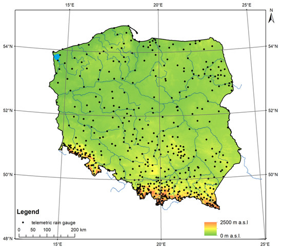
Figure 1.
Location of telemetric rain gauges in Poland.
2.1.2. Quality Control
The measurement data are affected by different kinds of errors. Therefore, the raw data must be quality controlled at different levels of data processing in real-time work [34]. The quality control procedures mostly depend on their intended application, but model-independent analysis has to be taken into account [35]. The simple automatic quality control (QC) methods are the commonly referred to plausibility tests that examine the range and variability of a given dataset [36,37,38].
High spatial and temporal variability of rainfall makes the definition of appropriate thresholds for QC tests a crucial issue: e.g., too low a threshold could make extreme values of precipitation not pass the test. Therefore, Fiebrich et al. [36] encourage the development of regionally specific thresholds for each applied test.
The developed and implemented QC procedures involve a five-stage check: gross errors, range check, temporal consistency check, spatial consistency check, and radar and satellite conformity check. If a sensor fails a particular check, its quality is reduced with a specified value. The output from this real-time quality control is quality index QIG of the data that indicates uncertainty in a particular measurement.
The automatic QC procedure for rain gauge data has been running in real time at IMGW since 2016. Otop et al. described and presented the preliminary version of the procedure [39]; however, it has been developed since then.
Gross error check (GEC). This first-stage check involves preliminary quality control which looks for gross errors mainly caused by the malfunctioning of measurement devices and by mistakes occurring during data transmission, reception and processing [35], which have strong effects on analyses. The aim of the GEC is to examine whether the precipitation values observed at i-gauge with s-sensor are within the physically acceptable range limits [34]: not less than 0 mm and not more than 80 mm during 10 min. The upper limit is set as a result of an analysis of long-term maximum values of 10-min precipitation accumulations measured at meteorological stations. Data from sensors that failed the check are rejected.
Range Check (RC). The second stage of the quality control applies climatic limits for precipitation amount. RC verifies the recorded data against the maximum values for a given location that is based on local climatological data. Taylor and Loescher [38] stated that thresholds determined by constructing statistical distributions based on existing data are more effective than simply using historical maximal values. In the QC procedure, the thresholds were defined as 10-min precipitation values with a 1% probability of exceeding.
Temporal Consistency Check (TCC) compares the precipitation accumulations from two sensors (heated and unheated) of the same rain gauge. Therefore, the TCC can only be performed in the warm part of the year when measurements from both sensors (heated, u, and unheated, uh) are available. The distinction between heated and unheated sensors is made, because this check is to detect the sensor malfunction due to mechanical failure. In the procedure, precipitation accumulations for a pre-set number of positively quality controlled observations are computed for both sensors: ΣGih and ΣGiuh. If the number of employed time steps is high enough and the difference between the two accumulations is below a pre-set threshold, then the both sensors pass the test.
Additionally, the detection of a constant value within a longer time interval is performed. If the same value is recorded for a certain period of time, then the sensor is regarded as partially or fully blocked.
Spatial Consistency Check (SCC) is applied to identify outliers based on a comparison to neighbouring gauges. There are several steps in the operational procedure of SCC. The calculation domain area is divided into basic sub-domains with a defined size. For each sub-domain, the following values are calculated: 25%, 50%, and 75% percentiles (respectively q25(G), q50(G), and q75(G)), and the median absolute deviation (MAD):
The criterion for the spatial consistency of i-gauge is implemented based on index Ii, which is calculated according to the formula from Kondragunta and Shrestha [40]:
The index is calculated for each sensor of a given rain i-gauge within the sub-domain and on this basis the 90%, 95%, and 99% percentiles of I are obtained (denoted as , etc.). A given sensor is identified as: (i) “weak outlier” if index is between , (ii) “outlier” if is between , and (iii) “strong outlier” if is higher than . The checking is analogically conducted for sub-domains moved a certain distance away in four directions. If the sensor is identified as an outlier in the basic sub-domain and all moved ones, then it failed the check.
Precipitation is highly variable in space and time; therefore, rain gauge data does not have to be spatially consistent, especially during convective conditions. For that reason, each sensor failing the check (i.e., identified as outlier) is additionally verified by means of quality-controlled radar data within the vicinity of the given gauge. If the ratio of gauge to mean radar rainfall is beyond defined limits, the result of the check is additionally confirmed and the gauge quality is reduced, depending on the level of outlying (“weak” or “strong outlier”) and level of disparities after verification by radar data.
Radar and Satellite Conformity Check (RSC). This last test is conducted to eliminate false gauge-reported precipitation. The RSC compares every sensor value Gi reporting rain with both radar and satellite observations (see Section 2.2 and Section 2.3) at the gauge vicinity. If the two verifying data are available and indicate “no precipitation” (0 mm) with qualities above pre-set thresholds, then the precipitation measured by a rain gauge is assumed to be erroneous and set to 0 unless the station is located in mountains or uplands, gauge data are available from both sensors, and the observations are similar.
QI value assignment. Initially, a sensor quality index is set to 1.0. If a sensor fails a particular check, its quality is reduced with an empirically determined value. Finally, data from a sensor with higher quality are chosen as a correct value and denoted as Gi, and, if the two qualities are equal, then the heated sensor Gih is preferable.
2.1.3. Spatial Interpolation
The point character of rain gauge measurements and the sparseness of operational networks make these measurements inadequate for providing sufficient information on the spatial distribution of precipitation. Therefore, rain gauge data after quality control are processed in order to provide precipitation field Gint.
There are two main types of methods concerning the spatial interpolation of meteorological elements: deterministic and geostatistical. The deterministic methods include, among others, inverse distance weighting (IDW) [41], Thiessen polygons, and polynomial interpolation. In contrast, the geostatistical methods are based on statistical models and give a direct opportunity for the evaluation of the estimation error [6,42,43]. They include methods that are based on various versions of a Kriging algorithm. In this work, both approaches were implemented and tested.
The usefulness of different versions of geostatistical methods depends on the nature of the analysed meteorological situation, the density and the distribution of the measurement gauges, and their qualities. In this work the following three versions have been tested: Ordinary Kriging, Universal Kriging, and Block Kriging, employing one of three semi-variogram models: Gaussian, spherical, and exponential. The whole domain is divided into 4 × 4 sub-domains (of 200 km × 225 km) and the empirical semi-variogram is determined for each of them employing least squares method in order to consider the spatial changeability of a precipitation field.
The abovementioned interpolation techniques were verified on data from July 2015 by: (i) random selection of about 10% of all rain gauges, excluding them from the interpolation, and comparison of their observations to values interpolated at their locations and (ii) comparison of daily accumulations with observations from climatological rain gauges. The Ordinary Kriging with exponential semi-variogram was empirically found to be optimal.
2.1.4. Quality Field
The spatially distributed quality index field QIG of the estimated precipitation field Gint is determined on the basis of data from point telemetric rain gauges, taking the two quality factors into consideration: (i) qualities of all gauges expressed by their QIs and (ii) density of the gauge network and completeness of data expressed by distance to the nearest gauge.
Point values of quality index QIGi for particular gauges are determined using quality algorithms presented in Section 2.1.2. Subsequently, the values are spatially interpolated into QIGint(x,y) field while using the same interpolation algorithm that was employed to precipitation data Gi interpolation. The local density of a rain gauge network is expressed by distance to the nearest gauge with a quality higher than a pre-set threshold. Having determined the distance for each pixel (x,y), the final quality field is obtained from the formula:
2.2. Weather Radar Network
2.2.1. Measurements (POLRAD Radar Network)
The weather radar data employed in the paper are generated by the Polish radar network POLRAD. The network consists of eight C-band Doppler radars from Leonardo Germany GmbH (formerly Gematronik and Selex) [44]. Three of them are dual-polarization radars; the others will be upgraded in the near future (Figure 2). Three- and two-dimensional radar products are generated by Rainbow 5 software every 10 min with a 1-km spatial resolution within a 215-km range. The Marshall-Palmer formula is used for the transformation of the reflectivity values measured by radar into the precipitation rate as the most common form of this relationship [45].
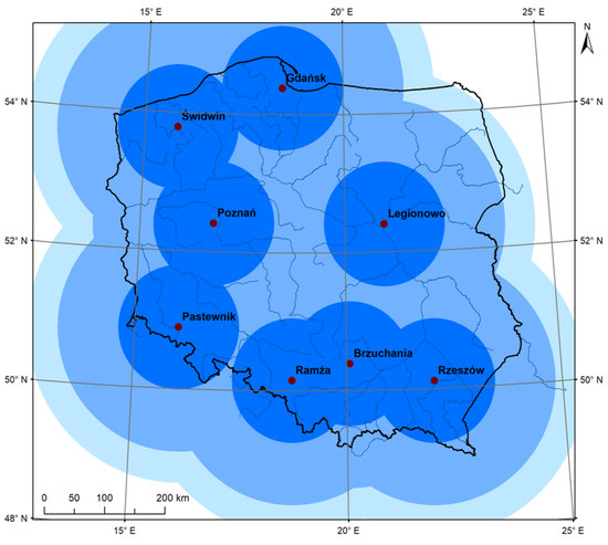
Figure 2.
Coverage by weather radar network POLRAD with 100-, 200-, and 250-km range.
2.2.2. Quality Control
Radar observations are burdened with a wide spectrum of errors from different sources—these are characterized by specific properties, spatial and temporal structures. Therefore, quality control aiming at the removal of detected errors and the quantitative characterization of data uncertainty is a crucial task in radar data processing. A review of the different sources of uncertainty can be found in numerous papers, e.g., [27,46].
The quality control of raw three-dimensional (3D) data volumes of the radar reflectivity is performed by means of the dedicated RADVOL-QC system, which was designed at IMGW to correct the data and generate quality fields QIR [27,47]. It was mainly developed in the frame of the BALTRAD project [48]. Since 2014, the system has worked operationally together with Rainbow 5 software.
The different kinds of errors taken into consideration by the RADVOL-QC system can be divided into several groups. The first one is connected with radar beam geometry and scan strategy and it includes effects that are related to the increasing distance from the radar site, such as the beam broadening and greater distances between neighbouring bins (measurement points). An additional source of uncertainty is the increasing distance of the radar beam to the earth’s surface because of the curvature and topography of the planet.
The next group, which, in practice, influences the radar estimates to the highest degree, is contamination by non-meteorological echoes. The echoes may be mainly caused by: (i) ground clutter (echoes from high objects close to the radar site), (ii) electromagnetic interference with the sun or external microwave emitters, which are usually visible in a radar image in the form of spikes pointing towards the radar site, (iii) speckles caused by measurement noise, and (iv) biological objects, such as birds or insects.
Other groups of errors result from: (i) beam blockage on terrain (mountains) resulting in a decrease of radar signals, (ii) attenuation in rain, especially in heavy rain, and (iii) anomalous propagation of the radar beam which causes, e.g., echoes received from non-meteorological and meteorological objects (terrain and hydrometeors, respectively) located outside the radar range.
Each category of errors is corrected by a dedicated quality control technique and, in consequence, is characterized by means of an individual quality index, and then the total quality is quantitatively computed by aggregation of all the individual indices into one total QIR while using a multiplicative scheme [25]. The fields of radar data quality index are assigned to each radar precipitation product. It should be emphasized that the quality index is reduced even though the radar observation after correction due to detected error is improved, because each correction leaves some uncertainty in the data.
The results of the RADVOL-QC verification and its effectiveness for the Polish weather radar network are presented and discussed in the paper by Ośródka et al. [27]. This system was significantly rebuilt and extended in 2018–2020.
2.2.3. Precipitation Estimation
The 3D volumes—quality controlled by the RADVOL-QC—are transformed by Rainbow 5 software into a set of specific two-dimensional (2D) products. The surface precipitation product is derived as PseudoSRI (surface rainfall intensity), i.e., cut-off at a constant height above ground level or from the lowest elevation out of the SRI range. Finally, a 10-min precipitation accumulation product is generated from two consecutive PseudoSRI products employing a rain tracking algorithm to take account of spatial and temporal interpolation in order to avoid effects that are related to data sampling. In this way, radar precipitation fields Rraw are operationally generated.
As mentioned above, radar measurement gives very good spatial representation of precipitation but suffers from several sources of errors. In order to improve the accuracy, the radar data are adjusted to rain-gauge observations, which provide more accurate point values [3,49]. Before radar compositing, individual radar data were subject to a preliminary mean field bias correction to reduce systematic errors, such as differences in calibration and, in consequence, under- or overestimation, and to unify all radars throughout the network. The bias adjustment factor is calculated individually for each radar and for each time step. The factor is calculated from a comparison of total amounts of collocated radar and rain gauge precipitation values with quality above a pre-set threshold and it is constant for the whole range of each radar.
Having data from individual weather radars, the composite is generated while using a quality-based approach. The method employs a combination of the data quality information and distance from the radar site as a criterion for data merging in overlapping areas. Moreover, the relevant composited quality field is determined for each pixel in the same way. The software was developed in IMGW by the authors since the Rainbow system dedicated to radar data processing does not work with quality information [50].
The spatial adjustment factor, determined at each time step from a comparison of past radar estimates with corresponding rain-gauge data, was introduced in order to handle non-uniform bias within the radar composite domain. The assumption is that rain gauge data correctly represents the precipitation at a longer time scale [51], at least of a few hours, so firstly both radar and rain gauge data are accumulated over a set of the following moving windows: 6, 24, and 120 h. The shortest period for which the relevant accumulation exceeds a pre-set threshold is applied to reflect the current characteristic of the precipitation field. The adjustment factor for each pixel of the field is derived from interpolation by means of the inverse distance method.
The unbiased precipitation field R obtained in this way is an input to the combination algorithm.
2.3. Meteorological Satellite
2.3.1. Measurements (Meteosat) and NWC SAF Processing
Passive and active microwave sensors are only available at low-earth orbits, so their temporal sampling and spatial resolution are limited to several hours and 8–40 km, respectively. Therefore, the use of data from the Meteosat Second Generation geostationary satellite working in rapid scan mode is the only possible solution for obtaining real-time precipitation information. Meteosat-based precipitation products can use only available visible (VIS) and infrared (IR) channels of the SEVIRI instrument [52]. However, the relationship linking IR brightness temperature and precipitation rate is indirect, since the IR channel is only sensitive to the cloud-top structure, so the measurements are qualitative and applicable mostly to convective precipitation.
The basis for the generation of the satellite-based precipitation field from the Meteosat observations is software delivered by the NWC SAF (Satellite Application Facilities on Support to Nowcasting and Very Short Range Forecasting), which is a program of EUMETSAT (the European Organisation for the Exploitation of Meteorological Satellites) (http://www.nwcsaf.org/). This software generates, inter alia, products related to precipitation [53].
The first two products are constructed from IR, and also—during daytime—from VIS spectral channels, so the products are available 24 h per day. Special attention is given to the VIS channel albedo, which is most correlated with precipitation intensity and implicitly contains information on the microphysical properties at the cloud top, such as effective radius and cloud phase. The CRR product (Convective Rainfall Rate) was developed to deliver information on precipitation rate from convective clouds and associated stratiform clouds, since cloud-top features in IR and the difference between WV (water vapour) and IR channels (usually used for the detection of high convective clouds) are applied in the product. The PC product (Precipitating Clouds) gives the total likelihood of precipitation without estimation of precipitation rate [54,55,56].
The last two products require both VIS and IR channels, so their generation is limited to daytime when the sun’s elevation is above 20°. The PC-PH product (Precipitating Clouds from Cloud Physical Properties) delivers information regarding the probability of the occurrence of precipitation with an intensity higher than 0.2 mm h−1. The algorithm is based on microphysical properties of clouds: droplets effective radius in the upper layer and the optical thickness of the cloud. The CRR-PH product (Convective Rainfall Rate from Cloud Physical Properties) delivers information regarding precipitation rate (in mm h−1) from convective clouds as well as stratiform clouds that are associated with convective systems. The product is similar to CRR, but additionally ingests information on microphysical cloud properties: water phase for cloud tops, effective radius of droplets, and optical thickness of cloud for rainfall determination [54,55,56].
2.3.2. Precipitation Estimation
The final satellite-based precipitation estimate is based on operational products that are generated by NWC SAF software from Meteosat rapid scan data available every five minutes. Generally, comparison with radar and rain gauge observations indicates better agreement with the “physical” products of CRR-PH and PC-PH than with those of CRR and PC. Unfortunately, the physical products are not available 24 h per day, so different algorithms are employed during the day and night.
For daytime, when the sun’s elevation is above 20°, the CRR-PH and PC-PH products are employed. Generally, intensive precipitation related to convective and thick stratiform cloud is well represented by the CRR-PH product, whereas the light precipitation must be replaced with probabilities that are provided by the PC-PH product scaled in precipitation 10-min accumulation (PC-PHaccum). After comparison with rain gauge observations, the following formula for daytime satellite precipitation Sday was empirically established:
These satellite products are only available at night; they are based on observations in the thermal IR part of the spectrum, so only CRR and PC products are employed. The CRR is used as an estimate of convective precipitation, whereas for the remaining areas covered by precipitation the PC product scaled from precipitation probability (0–100%) to 10-min precipitation accumulation PCaccum is employed instead. It is assumed that for probabilities in the range 0–20% “no precipitation” is observed and, for higher values, an empirically determined linear transformation is performed:
The round-the-clock satellite-based ground precipitation S is estimated from daytime or nighttime algorithms depending on the sun’s current elevation for each domain pixel. Examples of the estimates with relevant source NWC SAF products are depicted in Figure 3 for daytime and in Figure 4 for nighttime.
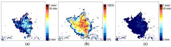
Figure 3.
Example of precipitation accumulation estimated from Convective Rainfall Rate from Cloud Physical Properties (CRR-PH) and Precipitating Clouds from Cloud Physical Properties (PC-PH) products employing the daytime algorithm (17 May 2014, 08:00 UTC): (a) CRR-PH transformed into 10-min accumulation (in mm), (b) PC-PH (precipitation probability in %), and (c) 10-min precipitation accumulation Sday (in mm).
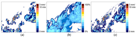
Figure 4.
Example of precipitation accumulation estimated from Convective Rainfall Rate (CRR) and Precipitating Clouds (PC) products employing the nighttime algorithm (16 May 2014, 00:00 UTC): (a) CRR transformed into 10-min accumulation (in mm), (b) PC (precipitation probability in %), and (c) 10-min precipitation accumulation Snight (in mm).
At the middle latitudes, images from geostationary orbit require correction due to the significant impact of the parallax effect. For the area of Poland it is highly recommended that data are shifted to a SSW direction, up to 25 km for the highest clouds. The correction of a position due to the parallax effect is performed while using an algorithm specified in software recommended by Convection Working Group of EUMETSAT (e.g., [57]) and based on the Cloud Top Height product of NWC SAF.
Since Meteosat satellite-derived precipitation fields are characterized by a 5–6 km spatial resolution over the area of Poland, they are downscaled into 1 km × 1 km pixels using the nearest neighbour technique, which was found the most effective for this purpose. Then aggregation into 10-min accumulations is performed employing two consecutive 5-min observations of the precipitation rate.
2.3.3. Quality Field
Quality index for satellite-based precipitation QIS is determined from empirical relationships based on analyses of satellite-based products and related rain gauge observations. For daytime (sun elevation ≥ 20°), the QIS is derived from CRR-PH and PC-PH products:
In general, at the daytime, the precipitation derived from CR-PH and PC-PH is more accurate than that at night, because the CRR and PC products are only based on information from IR channels.
3. Conditional Combination Technique Based on Quality Information
3.1. Algorithm Description
The investigation focused on the development of a technique for the combination of data provided by a telemetric rain gauge network, weather radar network, and meteorological satellite in order to obtain a quantitative precipitation estimate, i.e., an optimal precipitation field as close to the ground truth as possible. Altogether, these techniques are largely complementary in terms of their ability to detect and quantitatively characterize precipitation, spatial, and temporal resolution, and measurement range and errors, so the combination method should extract the strength of each measurement technique while minimizing its limitations. Bearing in mind that a combination of precipitation fields from the multi-source data must be treated as a final step in the processing chain of particular inputs, it is important to apply all of the available corrections beforehand, as uncorrected errors in the data will affect the quality of the final estimation [5].
In this work the conditional combination technique proposed by Sinclair and Pegram [17] is adapted for the merging of precipitation data. In this approach, rain gauges are trusted to measure precipitation accurately, but only in discrete points, whereas weather radar and satellite provide information regarding the spatial distribution of precipitation. This takes advantage of each instrument: accurate measurement of rain gauges at the point, high spatial resolution of precipitation derived from radar, and complete spatial coverage provided by satellite. The characteristic feature of the method, developed in the frame of the RainGRS system and hereafter referred to as “quality-based conditional merging”, is the key role of quality information that is generated in the form of maps of the quality index, QI, assigned to each precipitation field.
All of the precipitation fields: spatially interpolated rain gauges Gint, weather radar data after adjustment to rain gauges R, and Meteosat satellite S, together with assigned quality fields QIG, QIR, and QIS, are generated and processed according to algorithms described in previous section. The developed combination algorithm is divided into two stages: at first radar and satellite estimates are merged with rain gauge data separately, producing GR and GS fields respectively, and then they are combined into a final GRS precipitation field.
First, the rain gauge values are interpolated at radar pixel resolution, employing the Ordinary Kriging method, in the same configuration, as described in Section 2.1.3, to obtain an unbiased estimate of precipitation. The radar values at rain gauge locations and the same method of interpolation are used to get the interpolated radar field. Subsequently, the deviation between the measured and interpolated radar value (R – Rint) is computed and added to the rain gauge interpolated value at each pixel of the domain, according to the following formula:
It can be noted that the accuracy of the computed estimate depends on the distance to the nearest available rain gauge, and the radar precipitation field is preferable in the case of the low density of the rain gauge network [58]. Therefore, the resulting precipitation field RG is recombined with the radar precipitation field, applying the weighted scheme, which takes care of the quality of individual precipitation fields to obtain a combined GR field:
A combined gauge-satellite field GS is obtained analogically to the above procedure, where the satellite data S and relevant quality field QIS are taken, but not raised to the 7th power (this exponent was chosen empirically).
The satellite-derived precipitation estimate is indirectly obtained and it has generally lower quality, but provides the only source of information about spatial precipitation distribution out of radar composite range. Moreover, it is very useful in pixels where radar data has low quality due to a long distance to the nearest radar site or errors that are associated with factors, such as beam blockage or contamination by non-meteorological echoes. Therefore, the final quantitative precipitation estimate (GRS) is a combination of gauge-radar and gauge-satellite fields computed by means of the following weighted formula:
In the cases when rain gauge data Gint is not available, the final GRS field is determined from Formula (10) in which the GR and GS are replaced by R and S fields, respectively.
The quality index field QIGRS for the combined GRS precipitation is determined as a weighted mean from particular QIG, QIR, and QIS values:
3.2. Example
In Figure 5, particular precipitation fields (as 10-min accumulations) from 22 May 2019, 14:20 UTC are shown based on data from: the rain gauge network (Gint), weather radars (R), and Meteosat satellite (processed by the daytime algorithm) (S); these were generated while using the proposed quality-based techniques. The example represents a convective weather situation. It is observed that precipitation patterns of the fields are relatively similar, except for interpolated rain gauge data, which provides poor information regarding the spatial distribution of precipitation. The fields can differ in terms of magnitudes, especially in the case of satellite data; however, the data are a valuable supplement when other data are not available or their qualities are very low.
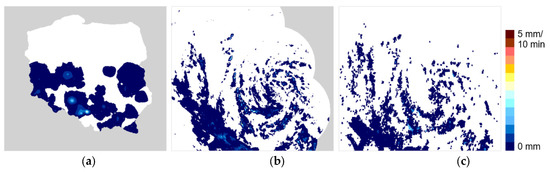
Figure 5.
Precipitation fields (as 10-min accumulations) for the area of Poland, 22 May 2019, 14:20 UTC: (a) precipitation fields: rain gauge (Gint), (b) weather radar (R), and (c) Meteosat satellite (S).
Figure 6 presents the QI fields for the particular precipitation data from Figure 5. In contrast to precipitation, the QI spatial patterns are extremely different. This is the effect of a quite different error structure of the data, as described in Section 2.
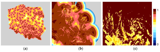
Figure 6.
Quality fields assigned to the precipitation data from Figure 5, 22 May 2019, 14:20 UTC: (a) QI fields for precipitation data: rain gauge (QIG), (b) weather radar (QIR), and (c) Meteosat satellite (QIS).
In the case of the rain gauge data, first of all the quality depends on the distance to the closest gauge and its individual quality. The obvious effect observed in the gauge-based field is that the network cannot detect all smaller size precipitation objects. Moreover, spatial interpolation resulted in areas around gauges that were detecting precipitation where estimated precipitation was stretched out.
For radar data, the impact of the main factors disturbing measurements is clearly noticeable, such as rings related to the distance to the radar site and height of the radar beam above the earth’s surface and, moreover, the presence of non-meteorological echoes, especially from RLAN signal interference in the form of so-called spike echoes, which are radially pointed towards radar sites [59]. In mountainous area in the south of Poland, decreased quality due to blockage on the terrain is also visible.
For satellite data, it is noticeable that high values of the quality index are connected with situations when satellite products do not detect precipitation.
Figure 7 presents a combined precipitation field GRS along with its quality field QIGRS. It is clearly visible that the quality of precipitation data strongly decreases with distance to the national borders because of the location of rain gauges and the radar network range.
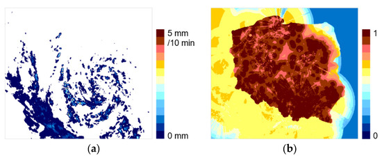
Figure 7.
Result of RainGRS combination for the area of Poland, 22 May 2019, 14:20 UTC: (a) combined precipitation field GRS, (b) relevant quality field QIGRS.
The QI value reflects the quality of a given type of precipitation field in the range between 0 and 1 without taking into account the overall quality of the measurement technique that was employed. Thus, it happens that the QI for the GRS field may be lower in some pixels than for any of the input fields, which can be seen by comparing Figure 6 and Figure 7b.
4. Results
4.1. Validation Criteria
The performance of the multi-source combination method was assessed while using independent measurements, which were not involved in the merging process and were derived from the climatological gauge network consisting of 344 stations; data from climatological gauges located at the same places as telemetric ones, were excluded from our data set (Figure 8). The validation was performed by comparing the observed daily precipitation for each control gauge to the collocated pixel in the accumulated 24-h precipitation field for each technique: interpolated rain gauges, radar, satellite, and multi-source combination. Only records with non-null data for a given control rain gauge and for all techniques were included in the analysis. Additionally, records with no rain registered by the control gauge were discarded.
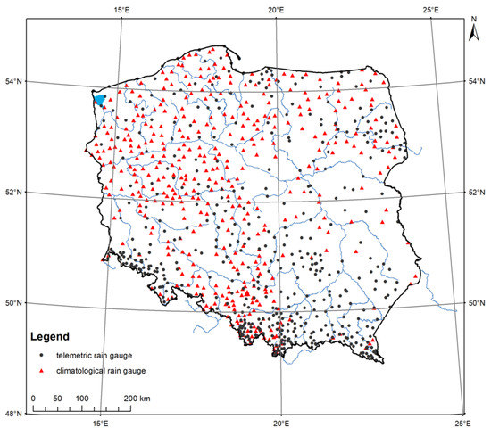
Figure 8.
Networks of climatological and telemetric rain gauges in Poland.
The rainfall variability in time and space varies significantly, depending on the season, from widespread precipitation during stratiform events in winter to very small-scale precipitation during convective events in summer. Therefore, for the validation process, the following months were selected as being representative: December 2018 as a typical month for winter when widespread snow prevailed; April 2019 when widespread precipitation predominated in the form of rain rather than snow; and, July 2019, with very heavy convective precipitation events.
In the literature, there are several quality metrics employed in the validation analysis. Pearson’s correlation coefficient, which is sensitive to a linear relationship between two variables, is defined as:
Root relative square error (RRSE) is based on variance, similarly to root mean square error, which is the most common metric used in verification studies as a good measure of accuracy, but it is scale-independent:
4.2. Dependence on Season
Analysing the results of the GRS field validation (Figure 9), it is clearly visible that satellite-based precipitation is less reliable than the other estimates. The slightly better results are observed for April and July 2019 when more satellite estimates are generated while using the daytime formula, i.e., involving data from both visible and infrared channels thanks to the higher elevation of the sun. In spite of the lowest quality, the satellite input provides valuable information in these areas, where other data are not available due to limitations in range or possible failures. Thus, they have little impact on the results of the analysis made herein, because all of the control gauges are located within the area of Poland where data from telemetric rain gauges are available and the coverage from weather radars is also quite good.
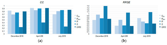
Figure 9.
Monthly values of quality metrics: (a) correlation coefficient (CC), (b) root relative square error (RRSE), for particular precipitation fields: interpolated rain gauges (Gint), raw radar (Rraw), unbiased radar (R), satellite (S), and merged (GRS). The values are obtained for three months from different seasons: winter (December 2018), mixed (April 2019), and summer (July 2019).
When it comes to radar estimates, the comparison of corrected radar rainfall fields against raw radar-derived precipitation highlights the significant ability of rain gauge adjustment to reduce errors observed in radar data. The correlation coefficient increased by 4–9%, while RRSE, which is more sensitive to bias, was reduced by 15–40%.
The verification results indicate that there are evident disparities between the reliabilities of precipitation estimates produced by all techniques: interpolated rain gauges, radar, radar after rain gauge adjustment, satellite, and multi-source combination, depending on the season.
For December 2018, the month of the cold part of the year when snowfall from stratiform clouds predominated, the precipitation estimates with rain gauges only (Gint) gave the best scores with a CC value of 0.83 and RRSE value of 0.69. Thus, it seems that the density of rain gauges and their spatial distribution are sufficient to reflect the variability of widespread precipitation. In turn, the radar derived estimates (Rraw) are clearly worse, even the corrected ones (R): after rain gauge adjustment the CC increased from 0.69 to 0.77, whereas RRSE was reduced from 0.97 to 0.78. This is caused by the geometry of the radar beam propagation and the fact that the weather radar more often samples above the tops of stratiform clouds, which are lower than convective clouds. In consequence, the reliability of the multi-source combination (GRS) is slightly worse than that rain gauge data alone; however, in comparison to radar data alone is a little better. The CC and RRSE values for GRS are equal to 0.8 and 0.76, respectively.
For April 2019, when also stratiform precipitation prevailed but rather rain than snow, it can be observed that Gint, R, and GRS seem to work comparably. Correlation coefficient values are quite good and change within a very small range from 0.91 to 0.92 and, similarly, the RRSE values vary from 0.40 to 0.42. It is important to notice the significant improvement in radar estimates after rain gauge adjustment: CC grew from 0.84 to 0.91 while RRSE decreased from 0.71 to 0.42.
There is a completely different situation in July 2019, which was a month with very heavy rain connected with convective events. In accordance with expectations, the rain gauge network turned out to be too sparse to capture the spatial variability of precipitation at the convection scale. It is worth pointing out that the interpolated rain gauge field (CC = 0.70 and RRSE = 0.79) was even less reliable than raw radar rainfall fields (CC = 0.81 and RRSE = 0.62). The verification results revealed that the weather radar is invaluable source of information when convective precipitation occurs. However, in this case, the impact of rain gauge adjustment on the reliability of radar-derived estimates was relatively small: the correlation coefficient increased to 0.85 and RRSE was reduced to 0.53. Blending information, on the one hand, the precipitation pattern from radar and, on the other hand, the point accuracy of the rain gauge network, causes the reliability of multi-source combination to outperform the reliabilities of all individual inputs, taking account of both metrics: CC and RRSE values for GRS are equal to 0.86 and 0.52, respectively.
Summarizing, these results suggest that a combination taking advantages of measurements from each device (registering the same phenomenon with different resolutions in time and space) provides precipitation estimates with reliability that is less dependent on a spatial scale of precipitation events and their dynamics.
4.3. Dependence on Input Data Qualities
One of the most important features of the presented scheme of multi-source precipitation data merging is the use of quantitative information about the quality of individual input data in each pixel of the computational domain. Therefore, the crucial problem is not only to correctly determine the spatial distributions of their qualities expressed by quality indices QIs, but also to synchronize their values, i.e., if inputs introduce similar uncertainties into the combined field then the QI values should also be similar. This is difficult, because the inputs are characterized by quite different error structures that change dynamically.
The quality metrics for GRS estimates against the control gauges were computed in a function of qualities of both data sources in order to illustrate how qualities of both radar and interpolated rain gauge data influence the reliability of multi-source estimates. The analysis was performed on the data from all three investigated months jointly in order to ensure a sufficient amount of data in every quality class. Additionally, values on the surface chart were averaged in fixed size grids to make the chart more readable.
In Figure 10 two diagrams show the dependence of the final field reliability—expressed by the quality metrics CC and RRSE—on qualities of the two main input fields: rain gauge (QIG) and radar (QIR). The relatively high correctness of the algorithms for determining these qualities is confirmed by the increasing reliability of the resulting GRS field, with both qualities and the symmetry of the chart about the QIG = QIR line.
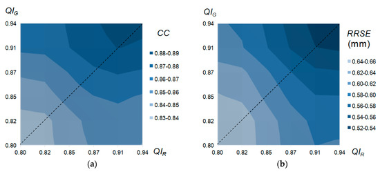
Figure 10.
Impact of rain gauge and radar data qualities on reliability of merged GRS precipitation field: (a) correlation coefficient (CC), (b) root relative square error (RRSE). Data from three months: December 2018, April and July 2019.
The influence of particular input data qualities on the reliability of the multi-source estimates depending on the season is depicted in Figure 11 and Figure 12. The control gauges were again divided into the quality classes for each investigated month, taking account of qualities of radar data and interpolated rain gauges in collocated pixels separately. As expected, the results are quite different for each month, which indicates that relationships between quality metrics of particular estimates and the input data QIs depend on the spatial and temporal characteristics of the precipitation fields—so, in consequence, on the season.
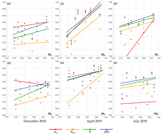
Figure 11.
Diagrams of monthly values of correlation coefficient (CC) for particular precipitation fields: interpolated rain gauges (Gint), raw radar (Rraw), unbiased radar (R), and merged (GRS) depending on gauge data quality (QIG) at the top and radar data quality (QIR) at the bottom. The diagrams are obtained for winter (December 2018), mixed (April 2019), and summer (July 2019).
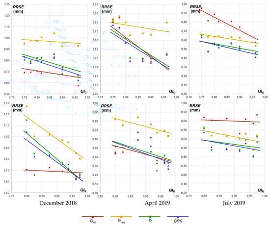
Figure 12.
Diagrams of monthly values of root relative square error (RRSE) for particular precipitation fields: interpolated rain gauges (Gint), raw radar (Rraw), unbiased radar (R), and merged (GRS), depending on gauge data quality (QIG) at the top and radar data quality (QIR) at the bottom. The diagrams are obtained for winter (December 2018), mixed (April 2019), and summer (July 2019).
Analysing the results for winter, it appears that the interpolated rain-gauge estimate is the best estimate independently for its quality, and the relationship between its accuracy and the quality index is hardly seen. The reliability of the multi-source combination is slightly better when the quality index of radar data is greater than 0.94, which is the equivalent of a distance to the radar site of below about 120 km, provided that radar data are not burdened with any errors and their quality index is only reduced due to the distance. It can be noted that radar data alone with such high quality is able to ensure the reliability of a precipitation field on the same level as interpolated rain gauges. For this month (December), the uncertainty of radar estimates increases when the quality index gets smaller, which is connected with the distance to the radar site to a large extent. In the case of the cold part of the year with widespread stratiform precipitation and when cloud tops are much lower than for convective precipitation, the weather radar is likely to overshoot the precipitation due to radar beam propagation geometry. The 120-km range seems to be a limitation to getting a precipitation radar estimate with an acceptable accuracy.
For summer, it is clearly visible that the interpolated rain gauge estimate is relatively inaccurate, with the calculated quality metrics strongly depending on its quality. The estimate is outperformed even by raw radar data and starts to have similar performance for quality index greater than 0.95, which corresponds to about a 5-km distance to the nearest rain gauge on the condition that the quality index is not decreased, due to the poor quality of a given rain gauge itself. Radar estimates, both raw and corrected, were found to have accuracy at a similar level, regardless of the radar data quality: the quality metrics change within a very small range. The reliability of the multi-source estimate is very close to the radar corrected one and tends to improve with the increasing quality of the interpolated rain gauge field. The results confirmed the conclusions from previous analysis that rain gauges are not able to reflect rainfall variability on a small scale and radar data provides more valuable information in summer.
In April, when widespread stratiform precipitation prevails with rain rather than snow, it can be noted that the differences in the reliability of particular estimates (Gint, R, GRS) are very small, regardless of the quality index for radar or interpolated rain gauge data. Similarly to the results for July, the accuracy of interpolated rain gauge estimates improves with their quality index. When it comes to radar estimates, this relationship is also observed, but, for raw radar estimates, it is stronger. In this month a significant improvement in radar estimates after rain gauge adjustment is noted.
5. Conclusions
This paper reports the proposed methodology to produce an estimated rainfall field as a result of multi-source precipitation data combination. There are great disparities between individual devices (rain gauges, radar, and satellite) in their quantitative characterization of precipitation in terms of: the measurement technique itself, spatial and temporal resolution, measurement range, and burdening errors. All of this affects the reliability of the combined field.
The developed method combines precipitation data from different sources with the assumption that rain gauges measure precipitation accurately at gauge locations, radar provides trustworthy spatial variability of precipitation with a high resolution, and satellite delivers information on precipitation distribution in areas out of the gauges’ and radar network’s ranges. The method enhances the reliability of input data by introducing the relevant quality fields.
The combination algorithm is divided into two steps. First, radar- and satellite-derived estimates are separately merged with rain gauge data, employing the conditional merging technique [17]. Since the reliability of the computed estimates depends on the distance to the nearest available rain gauge and radar or satellite data are preferable in the case of a low density of rain gauge network, so the computed estimates are recombined with a radar or satellite field, respectively, applying the weighted scheme taking the qualities of the fields.
In the next step, these estimates are combined into a final precipitation field using a weighted formula, in which weights depend on the distance to the nearest radar. This ensures that satellite data, which have the lowest quality, provide a combined field with information regarding the spatial distribution of precipitation practically only in these areas where radar data are not available due to limitations in range or possible failures of radar.
As the quality of input data plays a key role in the developed method, the quality control aiming at the detection and removal of errors and the quantitative characterization of the data uncertainty is a crucial task in input data processing. The quality fields for particular data sources are determined by employing different algorithms, because different quality factors have to be taken into consideration. Moreover, a synchronization among the quality fields for particular measurement techniques should be kept so that data for a given location coming from different sources, but expected to introduce similar uncertainties into the final field, should also have similar QI values.
The performance of the proposed method has been evaluated by comparing the measured daily precipitation from an independent climatological rain gauge network to the collocated pixel in the aggregated 24-h precipitation field for each technique: interpolated rain gauges, radar, satellite, and multi-source combination. Some months have been selected for the validation process, which are representative for widespread, mixed, and convective precipitation, respectively, as the spatial pattern of precipitation varies significantly across a year.
The verification results indicate that there are evident disparities among the reliabilities of precipitation estimates produced by particular techniques. It can be noted that satellite-based precipitation, generated by our own algorithm based on a set of NWC SAF products, is less reliable than the others. Better results are observed for satellite estimates that are produced when data from both visible and infrared channels are available—this is a serious limitation, because it is only for when the sun’s elevation is above 20°. Despite this, satellite provides valuable information in the area where there is no other data.
The comparison of raw and corrected radar-derived precipitation indicates that rain gauge adjustment significantly reduces the bias observed in radar data.
The analysis of the verification results shows that the accuracy of the multi-source combination strongly depends on the QIs of the input data and the type of precipitation. For heavy rain connected with convective events, the reliability of the multi-source combination, expressed by quality metrics, outperforms reliabilities of all particular inputs, regardless of their QIs. The combination reliability is very close to the reliability of radar corrected field and tends to improve with the increasing the QI of an interpolated rain gauge field. The interpolated rain gauge estimates are relatively inaccurate. Their quality metrics strongly depend on their QI and for QI greater than 0.95 have a similar performance as radar-derived estimates. This QI value corresponds to about a 5-km distance from the nearest rain gauge (on condition that the QI is not decreased due to the poor quality of a given rain gauge itself). It confirms that rain gauges are not able to reflect a spatial pattern of precipitation at a small scale, especially if rain gauge network is rather sparse. However, interpolated rain gauge estimates provide valuable input for the multi-source combination when the gauges are of high quality.
Quite a different situation occurs in the case of widespread precipitation. The reliability of the multi-source combination is slightly better than the reliability of individual techniques only when the QI of radar data is greater than 0.94, which is equivalent of a distance to the radar site of below about 120 km, provided that radar data is not burdened with any errors so that its QI is only reduced due to the distance. This is caused by the geometry of the radar beam propagation and the fact that the weather radar more often samples above the tops of stratiform clouds, which are lower than convective clouds.
Summarizing, the RainGRS system is an effective tool for the estimation of a high-resolution precipitation field. Important information in this estimation is provided by precisely determined quality indices of individual precipitation fields. However, its effectiveness depends on the type of rainfall and, therefore, on the season of the year.
Author Contributions
Conceptualization, A.J. and J.S.; methodology, A.J., I.O., J.S., P.S. and K.O.; software, A.J. and K.O.; validation, A.J., J.S., K.O. and I.O.; investigation, A.J. and J.S.; writing—original draft preparation, A.J. and J.S.; writing—review and editing, A.J., J.S. and K.O. All authors have read and agreed to the published version of the manuscript.
Funding
The RainGRS system was developed and implemented in the frame of the Institute of Meteorology and Water Management—National Research Institute statutory works.
Conflicts of Interest
The authors declare no conflict of interest.
References
- Michaelides, S.; Levizzani, V.; Anagnostou, E.; Bauer, P.; Kasparis, T.; Lane, J.E. Precipitation: Measurement, remote sensing, climatology and modeling. Atmos. Res. 2009, 94, 512–533. [Google Scholar] [CrossRef]
- Ebert, E.E.; Janowiak, J.E.; Kidd, C. Comparison of near-real-time precipitation estimates from satellite observations and numerical models. Bull. Am. Meteorol. Soc. 2007, 88, 47–64. [Google Scholar] [CrossRef]
- Gjertsen, U.; Šálek, M.; Michelson, D.B. Gauge-Adjustment of Radar-Based Precipitation Estimates; COST Action 717: Luxembourg, Belgium, 2004. [Google Scholar]
- Chumchean, S.; Seed, A.; Sharma, A. Correcting of real-time radar rainfall bias using a Kalman filtering approach. J. Hydrol. 2006, 137, 123–137. [Google Scholar] [CrossRef]
- Velasco-Forero, C.A.; Sempere-Torres, D.; Cassiraga, E.F.; Gómez-Hernández, J.G. A non-parametric automatic blending methodology to estimate rainfall fields from rain gauge and radar data. Adv. Water Resour. 2009, 32, 986–1002. [Google Scholar] [CrossRef]
- Sideris, I.V.; Gabella, M.; Erdin, R.; Germann, U. Real-time radar–rain-gauge merging using spatio-temporal co-kriging with external drift in the alpine terrain of Switzerland. Q. J. R. Meteorol. Soc. 2014, 140, 1097–1111. [Google Scholar] [CrossRef]
- Pereira Filho, A.J.; Crawford, K.C.; Hartzell, C. Improving WSR-88D hourly rainfall estimates. Weather Forecast. 1998, 13, 1016–1028. [Google Scholar] [CrossRef]
- Pereira Filho, A.J. Integrating Gauge, Radar and Satellite Rainfall. In WWRP International Precipitation Working Group Workshop; CGMS-WMO: Monterey, CA, USA, 2004. [Google Scholar]
- Šálek, M.; Novák, P.; Seo, D.-J. Operational application of combined radar and raingauges precipitation estimation at the CHMI. Proc. ERAD 2004, 2004, 16–20. [Google Scholar]
- Rosenfeld, D.; Wolff, D.B.; Amitay, E. The window probability matching method for rainfall measurements with radar. J. Appl. Meteorol. 1994, 33, 682–693. [Google Scholar] [CrossRef][Green Version]
- Sun, X.; Mein, R.G.; Keenan, T.D.; Elliott, J.F. Flood estimation using radar and raingauge data. J. Hydrol. 2000, 239, 4–18. [Google Scholar] [CrossRef]
- Piman, T.; Babel, M.S.; Das Gupta, A.; Weesakul, S. Development of a window correlation matching method for improved radar rainfall estimation. Hydrol. Earth Syst. Sci. 2007, 11, 1361–1372. [Google Scholar] [CrossRef]
- Krajewski, W.F. Cokriging of radar-rainfall and rain gage data. J. Geophys. Res. 1987, 92, 9571–9580. [Google Scholar] [CrossRef]
- Seo, D.-J. Real-time estimation of rainfall fields using radar rainfall and rain gage data. J. Hydrol. 1998, 208, 37–52. [Google Scholar] [CrossRef]
- Haberlandt, U. Geostatistical interpolation of hourly precipitation from rain gauges and radar for a large-scale extreme rainfall event. J. Hydrol. 2007, 332, 144–157. [Google Scholar] [CrossRef]
- Delrieu, G.; Wijbrans, A.; Boudevillain, B.; Faure, D.; Bonnifait, L.; Kirstetter, P.-E. Geostatistical radar-raingauge merging: A novel method for the quantification of rain estimation accuracy. Adv. Water Resour. 2014, 71, 110–124. [Google Scholar] [CrossRef]
- Sinclair, S.; Pegram, G. Combining radar and rain gauge rainfall estimates using conditional merging. Atmos. Sci. Lett. 2005, 6, 19–22. [Google Scholar] [CrossRef]
- Ehret, U.; Götzinger, J.; Bárdossy, A.; Pegram, G.G.S. Radar-based flood forecasting in small catchments, exemplified by the Goldersbach catchment, Germany. Int. J. River Basin Manag. 2008, 6, 323–329. [Google Scholar] [CrossRef]
- Todini, E. A Bayesian technique for conditioning radar precipitation estimates to rain-gauge measurements. Hydrol. Earth Syst. Sci. 2001, 5, 187–199. [Google Scholar] [CrossRef]
- Seo, D.-J.; Breidenbach, J.P. Real-time correction of spatially nonuniform bias in radar rainfall data using rain gauge measurements. J. Hydrometeorol. 2002, 3, 93–111. [Google Scholar] [CrossRef]
- Chappell, A.; Renzullo, L.J.; Raupach, T.H.; Haylock, M. Evaluating geostatistical methods of blending satellite and gauge data to estimate near real-time daily rainfall for Australia. J. Hydrol. 2013, 493, 105–114. [Google Scholar] [CrossRef]
- Todini, E.; Mazzetti, C. A Bayesian Multisensor Combination Approach to Rainfall Estimate. In Proceedings of the 2nd International Symposium on Communications, Control and Signal Processing, Marrakech, Morocco, 13–15 March 2006. [Google Scholar]
- Goudenhoofdt, E.; Delobbe, L. Evaluation of radar-gauge merging methods for quantitative precipitation estimates. Hydrol. Earth Syst. Sci. 2009, 13, 195–203. [Google Scholar] [CrossRef]
- McKee, J.L. Evaluation of Gauge-Radar Merging Methods for Quantitative Precipitation Estimation in Hydrology: A Case Study in the Upper Thames River Basin. Electronic Thesis and Dissertation Repository. Available online: https://www.semanticscholar.org/paper/Evaluation-of-gauge-radar-merging-methods-for-in-a-McKee/1590c42d0c5313ff362a2b60046f8021fd966d8f (accessed on 26 May 2020).
- Einfalt, T.; Szturc, J.; Ośródka, K. The quality index for radar precipitation data—A tower of Babel? Atmos. Sci. Lett. 2010, 11, 139–144. [Google Scholar] [CrossRef]
- Szturc, J.; Ośródka, K.; Jurczyk, A. Quality index scheme for quantitative uncertainty characterisation of radar-based precipitation. Meteorol. Appl. 2011, 18, 407–420. [Google Scholar] [CrossRef]
- Ośródka, K.; Szturc, J.; Jurczyk, A. Chain of data quality algorithms for 3-D single-polarization radar reflectivity (RADVOL-QC system). Meteorol. Appl. 2014, 21, 256–270. [Google Scholar] [CrossRef]
- Ośródka, K.; Szturc, J. Quality-based generation of weather radar Cartesian products. Atmos. Meas. Tech. 2015, 8, 2173–2181. [Google Scholar] [CrossRef]
- Jurczyk, A.; Ośródka, K.; Szturc, J. Research studies on improvement in real-time estimation of radar-based precipitation in Poland. Meteorol. Atmos. Phys. 2008, 101, 159–173. [Google Scholar] [CrossRef]
- Struzik, P.; Niedbała, J.; Sadoń, J. Validation of Satellite Precipitation Products with Use of Hydrological Models—EUMETSAT H-SAF Activities. In Proceedings of the 3rd IPWG Workshop on Precipitation Measurements, Melbourne, Australia, 23–27 October 2006. [Google Scholar]
- Martinaitis, S.M.; Cocks, S.B.; Qi, B.; Kaney, Y.; Zhang, J.; Howard, K. Understanding winter precipitation impacts on automated gauges within a real-time system. J. Hydrometeorol. 2015, 16, 2345–2363. [Google Scholar] [CrossRef]
- Michelson, D. Systematic correction of precipitation gauge observations using analyzed meteorological variables. J. Hydrol. 2004, 290, 161–177. [Google Scholar] [CrossRef]
- Einfalt, T.; Michaelides, S. Quality Control of PrecipitationData. In Precipitation: Advances in Measurement, Estimation and Prediction; Michaelides, S., Ed.; Springer: Berlin/Heidelberg, Germany, 2008. [Google Scholar]
- WMO. Guide to the Global Observing System. Available online: https://www.wmo.int/pages/prog/www/OSY/Manual/488_Guide_2007.pdf (accessed on 26 May 2020).
- Steinacker, R.; Mayer, D.; Steiner, A. Data quality control based on self-consistency. Mon. Weather Rev. 2011, 139, 3974–3991. [Google Scholar] [CrossRef]
- Fiebrich, C.A.; Morgan, C.R.; McCombs, A.G. Quality assurance procedures for mesoscale meteorological data. J. Atmos. Ocean. Technol. 2010, 27, 1565–1582. [Google Scholar] [CrossRef]
- Jatho, N.; Pluntke, T.; Kurbjuhn, C.; Bernhofer, C. An approach to combine radar and gauge based rainfall data under consideration of their qualities in low mountain ranges of Saxony. Nat. Hazards Earth Syst. Sci. 2010, 10, 429–446. [Google Scholar] [CrossRef]
- Taylor, J.R.; Loescher, H.L. Automated quality control methods for sensor data: A novel observatory approach. Biogeosciences 2013, 10, 4957–4971. [Google Scholar] [CrossRef]
- Otop, I.; Szturc, J.; Ośródka, K.; Djaków, P. Automatic quality control of telemetric rain gauge data for operational applications at IMGW-PIB. Itm Web Conf. 2018, 23, 00028. [Google Scholar] [CrossRef][Green Version]
- Kondragunta, C.R.; Shrestha, K. Automated real-time operational rain gauge quality-control tools in NWS Hydrologic Operations. In Proceedings of the 86th AMS Annual Meeting, Atlanta, GA, USA, 28 January–3 February 2006. [Google Scholar]
- Ahrens, B. Distance in spatial interpolation of daily rain gauge data. Hydrol. Earth Syst. Sci. 2006, 10, 197–208. [Google Scholar] [CrossRef]
- Dobesch, H.; Dumolard, P.; Dyras, I. Spatial Interpolation for Climate Data: The Use of GIS in Climatology and Meteorology; ISTE Ltd.: Newport Beach, CA, USA, 2007. [Google Scholar]
- Berndt, C.; Rabiei, E.; Haberlandt, U. Geostatistical merging of rain gauge and radar data for high temporal resolutions and various station density scenarios. J. Hydrol. 2014, 508, 88–101. [Google Scholar] [CrossRef]
- Szturc, J.; Jurczyk, A.; Ośródka, K.; Wyszogrodzki, A.; Giszterowicz, M. Precipitation estimation and nowcasting at IMGW (SEiNO system). Meteorol. Hydrol. Water Manag. 2018, 6, 3–12. [Google Scholar] [CrossRef]
- Neuper, M.; Ehret, U. Quantitative precipitation estimation with weather radar using a data- and information-based approach. Hydrol. Earth Syst. Sci. 2019, 23, 3711–3733. [Google Scholar] [CrossRef]
- Villarini, G.; Krajewski, W.F. Review of the different sources of uncertainty in single polarization radar-based estimates of rainfall. Surv. Geophys. 2010, 31, 107–129. [Google Scholar] [CrossRef]
- Szturc, J.; Ośródka, K.; Jurczyk, A. Quality Control Algorithms Applied on Weather Radar Reflectivity Data. In Doppler Radar Observations—Weather Radar, Wind Profiler, Ionospheric Radar, and Other Advanced Applications; Bech, J., Chau, J., Eds.; InTech: Rijeka, Croatia, 2012. [Google Scholar]
- Michelson, D.; Henja, A.; Ernes, S.; Haase, G.; Koistinen, J.; Ośródka, K.; Peltonen, T.; Szewczykowski, M.; Szturc, J. BALTRAD advanced weather radar networking. J. Open Res. Softw. 2018, 6, 12. [Google Scholar] [CrossRef]
- Bruen, M.; O’Loughlin, F. Towards a nonlinear radar-gauge adjustment of radar via a piece-wise method. Meteorol. Appl. 2014, 21, 675–683. [Google Scholar] [CrossRef]
- Jurczyk, A.; Szturc, J.; Ośródka, K. Quality-based compositing of weather radar-derived precipitation. Meteorol. Appl. 2020, 27, e1812. [Google Scholar]
- Berg, P.; Norin, L.; Olsson, J. Creation of a high resolution precipitation data set by merging gridded gauge data and radar observations for Sweden. J. Hydrol. 2016, 541, 6–13. [Google Scholar] [CrossRef]
- Mugnai, A.; Casella, D.; Cattani, E.; Dietrich, S.; Laviola, S.; Levizzani, V.; Panegrossi, G.; Petracca, M.; Sanò, P.; Di Paola, F.; et al. Precipitation products from the hydrology SAF. Nat. Hazards Earth Syst. Sci. 2013, 13, 1959–1981. [Google Scholar] [CrossRef]
- Tapiador, F.J.; Marcos, C.; Sancho, J.M. The convective rainfall rate from cloud physical properties algorithm for Meteosat Second-Generation satellites: Microphysical basis and intercomparisons using an object-based method. Remote Sens. 2019, 11, 527. [Google Scholar] [CrossRef]
- NWC SAF, User Manual for the “Precipitation Product” Processors of the NWC/GEO, Issue 1, Rev. 0, 21 January 2019. Available online: http://www.nwcsaf.org/web/guest/scientificdocumentation#NWCSAF/GEO%20Basic%20Documents (accessed on 26 May 2020).
- NWC SAF, Algorithm Theoretical Basis Document for the “Precipitation Product” Processors of the NWC/GEO, Issue 1, Rev. 1, 15 October 2016. Available online: http://www.nwcsaf.org/web/guest/scientificdocumentation#NWCSAF/GEO%20Basic%20Documents (accessed on 26 May 2020).
- NWC SAF, Scientific and Validation Report for the “Precipitation Product” Processors of the NWC/GEO, Issue 1, Rev. 0, 15 October 2016. Available online: http://www.nwcsaf.org/web/guest/scientificdocumentation#NWCSAF/GEO%20Basic%20Documents (accessed on 26 May 2020).
- Bieliński, T. A parallax shift effect correction based on cloud height for geostationary satellites and radar observations. Remote Sens. 2020, 12, 365. [Google Scholar]
- Velasco-Forero, C.A.; Seed, A.; Sempere-Torres, D.; Pegram, G. Optimal Estimation of Rainfall Fields Merging Radar and Rain Gauges Data in an Operational Context. In Proceedings of the 5th European Conference on Radar in Meteorology and Hydrology ERAD 2008, Helsinki, Finland, 30 June–4 July 2008. [Google Scholar]
- Saltikoff, E.; Cho, J.Y.; Tristant, P.; Huuskonen, A.; Allmon, L.; Cook, R.; Becker, E.; Joe, P. The threat to weather radars by wireless technology. Bull. Am. Meteorol. Soc. 2016, 97, 1159–1167. [Google Scholar] [CrossRef]
© 2020 by the authors. Licensee MDPI, Basel, Switzerland. This article is an open access article distributed under the terms and conditions of the Creative Commons Attribution (CC BY) license (http://creativecommons.org/licenses/by/4.0/).