Abstract
Spaceborne Global Navigation Satellite System Reflectometry (GNSS-R) provides a new opportunity for land observation. This study is the first to compare and evaluate the performance of the only two spaceborne GNSS-R satellite missions whose data are publicly available, i.e., the UK’s TechdemoSat-1 (TDS-1) and the US’s Cyclone Global Navigation Satellite System (CYGNSS), for sensitivity analysis with SMAP SM on a daily basis and soil moisture (SM) estimates on a monthly basis over Mainland China. For daily sensitivity analysis, the two data were matched up and compared for the period (i.e., May 2017 through April 2018) when they coexisted (R = 0.561 vs. R = 0.613). For monthly SM estimates, a back-propagation artificial neural network (BP-ANN) was used to construct a model using data from more than two years. The model was subsequently used to derive long-term and continuous SM maps over Mainland China. The results showed that TDS-1 and CYGNSS agree and correlate very well with the SMAP SM in Mainland China (R = 0.676, MAE = 0.052 m3m−3, and ubRMSE = 0.060 m3m−3 for TDS-1; R = 0.798, MAE = 0.040 m3m−3, and ubRMSE = 0.062 m3m−3 for CYGNSS). The retrieved results were further validated using monthly in situ SM data from dense sites across Mainland China. It was found that the SM derived from the TDS-1/CYGNSS also correlated well with in situ SM (R = 0.687, MAE = 0.066 m3m−3, and ubRMSE = 0.056 m3m−3 for TDS-1; R = 0.724, MAE = 0.052 m3m−3, and ubRMSE = 0.053 m3m−3 for CYGNSS). The results in this study suggested that TDS-1/CYGNSS and the upcoming spaceborne GNSS-R mission could be new and powerful data sources to produce SM data set at a large scale and with relatively high precision.
1. Introduction
Global Navigation Satellite System Reflectometry (GNSS-R) is a technique that exploits the capability of GNSS satellites to act as a bistatic-radar with the GNSS satellites as its transmitters and the receiver capable of processing scattered signals from the Earth’s surface [1,2]. With the development of spaceborne observations, the GNSS-R technology provides new opportunities for Earth observation on a global scale. The first spaceborne GNSS-R was launched on the UK-Disaster Monitoring Constellation (UK-DMC) satellite in September 2003, which proved that spaceborne GNSS-R signals can reliably measure environmental parameters for ocean and land surface [3,4]. The TechdemoSat-1 (TDS-1), the experimental GNSS-R satellite, launched in July 2014, has demonstrated the strong sensitivity of the GNSS-R signal to various ocean and land parameters [5,6,7,8,9]. However, TDS-1 has limitations in data acquisition, both spatially and temporally, because the TDS-1 contains only one GPS-R payload and active for two out of every eight days, and the payload of TDS-1 stopped transmitting data in December 2018. The Cyclone Global Navigation Satellite System (CYGNSS) mission, launched into space in December 2016, contains eight microsatellites with the same payload as the TDS-1. The CYGNSS was designed to measure ocean winds in the tropics, while reflections observed from the satellites were also proved sensitive to land parameters [10,11,12,13]. Table 1 shows general information of the TDS-1 and CYGNSS missions. Compared to TDS-1 (10–35 days) [14], the CYGNSS microsatellites randomly receive GNSS-R signals with revisiting times of approximately 2.8~7 h per day [12,15].

Table 1.
General Information of the TechdemoSat-1 (TDS-1) and Cyclone Global Navigation Satellite System (CYGNSS) missions.
Soil moisture (SM) has a significant impact on the earth’s ecosystem by affecting the hydrological processes and climate changes, and it also plays an important role in land surface evapotranspiration, water migration, and the carbon cycle [16,17]. This reveals the necessity to obtain and analyze SM information in the long-term and over a large scale for such applications. Common remote sensing approaches to measure SM on a large scale mainly rely on optical and microwave sensors [18,19]. Optical remote sensing data have high-spatial resolution (hundreds of meters) but are impacted greatly by cloud and mist. Passive microwave remote sensing data have high-temporal resolution (one or two half-orbit per day) with low-spatial distributions (tens of kilometers). Research results have shown methods to downscale the SM product from SM measurements (i.e., soil moisture ocean salinity (SMOS)) to obtain high-resolution SM maps at 1 km from the approximately 40 km native resolution of the instrument; this is closer to the spatial resolution achieved by GNSS-R instruments [20,21]. Spaceborne GNSS-R is an attractive approach for regional and global scale SM measurements because the GNSS signal is in the L-band, which is the same as the SM missions such as soil moisture active and passive (SMAP) and SMOS satellites, making it optimal for SM remote sensing [22,23]. Additionally, a constellation of GNSS-R receivers shortens the revisit time compared to traditional microwave remote sensing sensors.
Due to the abovementioned advantages of monitoring the SM with spaceborne GNSS-R, and in order to support the development of future GNSS-R satellites/constellations dedicated for monitoring the SM, many studies have focused on developing algorithms for SM estimation using the TDS-1 and CYGNSS observations [6,8,12,15,24,25]. Because TDS-1 and CYGNSS are both designed for ocean sensing, the data processing on land has inherent limitations, such as that they cannot receive adequate data from high altitude regions due to no consideration of land topography. Table 2 shows a summary of relevant studies using TDS-1 and CYGNSS to estimate SM. From Table 2, it can be concluded that notable gaps remain for evaluating use of the two data to estimate SM:
Table 2.
Summary of relevant studies using TDS-1 and CYGNSS to estimate SM. The “key results” column is summarized from the following two aspects: (1) key conclusion and (2) accuracy evaluations. N/A represents “not applicable”.
- (1)
- No study compares the current two existing spaceborne GNSS-R missions (i.e., TDS-1 and CYGNSS) whose data are publicly available. The two missions and their data have several common points (e.g., the same payload SGR-ReSI and the same key observable DDM SNR for SM sensing). Precisely because of this situation, the comparisons between them will bring new insights into better using their data and provide reference information for designation of future GNSS-R payloads for soil moisture sensing.
- (2)
- No attempt has been made to evaluate the performance of using the two data to estimate both daily and monthly SM, and a few studies focused on comparing the SM derived from CYGNSS with the SM derived from limited numbers of in situ sites.
Aiming to address the above-mentioned two issues, the overall objectives of this study are (1) for the first time ever to compare and evaluate the performance of the only two spaceborne GNSS-R satellite missions whose data are publicly available (e.g., TDS-1 and CYGNSS) for soil moisture estimations; and (2) comprehensively validates the GNSS-R derived soil moisture by taking advantage of the dense in situ networks over Mainland China. Specifically, the TDS-1 and CYGNSS data are matched up regionally and compared during their overlapping periods (i.e., May 2017 through April 2018). For daily sensitivity analysis, the effective reflected power (Pr,eff) and the surface reflectivity (SR) proposed by Chew et al. [6,12] were used as proxies to evaluate their ability to estimate SM. For the monthly SM estimates, to reduce vegetation and ground effects, a new SM retrieval algorithm combining variables affecting SM (i.e., vegetation cover, surface roughness, topography, and precipitation) and data for deriving SM (i.e., SR and SMAP SM data) were constructed based on the back propagation ANN (BP-ANN). The model was applied to compute long-term (over one year) and large-scale (a 50-km grid for TDS-1 and a 10-km grid for CYGNSS) SM data sets over Mainland China. Finally, the results were validated by the SMAP SM products and in situ data. The results of this study provide the possibility that TDS-1/CYGNSS and the upcoming spaceborne GNSS-R missions could be new and powerful data sources to produce SM data set with large scale and relatively high previse precision.
2. Data and Methods
2.1. Spaceborne GNSS-R Dataset
The study area is the region of Mainland China (73 through 135°E and 18 through 53°N), as shown in Figure 1. Data from TDS-1 and CYGNSS are used in this study. The two missions coexisted between the period from May 2017 to April 2018. TDS-1 level 1b data were downloaded via ftp.MERRByS.co.uk, and CYGNSS level 1 data, version 2.1, were downloaded via https://podaac.jpl.nasa.gov/. The DDM is the main observable of the data. One DDM is a two-dimensional image generated by the scatter power from the surface of the specular point with the surroundings. DDMs are computed with a locally generated replica for different path delays and Doppler shifts. The SNR is computed from the averaged values of several delay-Doppler bins around the peak, to the average noise floor computed for delay lags before the reflected signal. Since the CYGNSS on-board data compression algorithm has an elevation upper limit of 600 m [12,13], which thus makes the valid observations mainly distributed in the southeastern part of Mainland China. For TDS-1, the reflected waveforms from surface with elevations over 3000 m were excluded, as done previously [6]. The TDS-1 and CYGNSS data were then filtered for (1) the antenna gain greater than 0 dB (corresponding to uncertainties reported in the measured antenna gain patterns) [6] and (2) the elevation angle of the specular point higher than 30° (to keep the good-quality Left Hand Circularly Polarized (LHCP) data) [12]. Also, a parameter called DirectSignallDDM in the TDS-1 L1b data and Quality Flags (i.e., direct signal in DDM, low confidence in the GPS EIRP estimate) in the CYGNSS L1b data were used to select the good data acquisitions. The NASA Shuttle Radar Topographic Mission (SRTM) 90 m Digital Elevation Models (DEM) database was applied to compute the elevations of the TDS-1 and CYGNSS coverage areas.
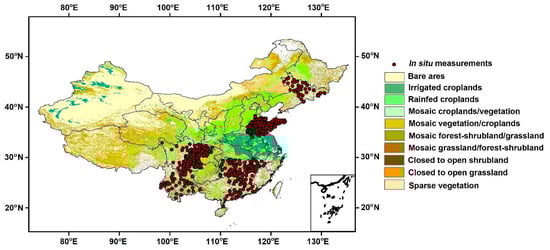
Figure 1.
Locations of the 588 in situ soil moisture (SM) sites in Mainland China. The background map is the Global Land Cover Map for 2009 (GLCover 2009) data set.
2.2. In Situ Measurements
Monthly averaged in situ SM data of 588 sites selected from the meteorological observation network of Mainland China were used for validation (Figure 1). Considering the complex geographical environment and climate conditions in China, the selected sites are distributed in seven provinces of China, with different land covers, climate conditions, and terrain distributions (Table 3). All the in situ SM data were collected at a depth of 10 cm. Additionally, as shown in Figure 1, to exclude the effects of vegetation cover, buildings, inland water bodies, etc., the selected sites were located in bare soil and low vegetated density regions (i.e., vegetation height < 5 m) identified by the Global Land Cover Map for 2009 (GlobCover 2009).
Table 3.
Characteristics of the in situ measurements.
2.3. Calculation of the Daily Surface Reflectivity (SR) and the Effective Reflected Power (Pr,eff)
For daily basis sensitivity analysis, the surface reflectivity (SR) and effective reflected power (Pr,eff) proposed by Chew et al. [6,12] are used as a proxy for SM to compare it with the SMAP SM products. The SR and Pr,eff are calibrated variables of SNR after correcting effects such as antenna gain, receiver noise, and range items. The SR and Pr,eff depend on the reflectivity of the soil, which is related to the dielectric constant [26,27].
For TDS-1 data, as presented by Carreno-Luengo et al. [26] and Chew et al. [6], the effective reflected power (Pr, eff) is defined as the corrected SNR of the DDM, as shown in Equation (1). The SNR (in dB) correction is based on the bistatic radar equation describing the coherent component of the received power.
where SNR is the peak power minus the noise, Rts is the range from the transmitter to the specular reflection point, Rsr is the range from the specular reflection point to the receiver, Gr is the antenna gain toward the specular reflection point, and is the incidence angle.
For CYGNSS data, Chew et al. [12] proposed that the SR (in dB) can be described as follows:
where Ptr is the transmitted power, Gt is the gain of the transmitting antenna, and λ represents wavelength of the GPS L1 bands signal (0.19 m).
2.4. Monthly SM Estimation Using Neural Network
GNSS-R reflectivity is sensitive to SM and to other geophysical parameters, e.g., vegetation canopy, elevation, slope, surface roughness, and precipitation [28,29,30,31]. Thus, for monthly SM estimates, a new model considering the aforementioned variables was constructed using the BP-ANN to estimate continuous SM over the study area (Figure 2). The BP-ANN is a supervised learning algorithm, which refers to a multi-layers forward neural network with an input layer, one or more hidden layers, and an output layer. BP-ANN can be used in many tasks, e.g., classification and regression [32,33], and is also used in the geoscience field [34]. BP-ANN can, in principle, efficiently handle input and output variables relations, with no limited in linear relationships [35,36]. A multifactor non-linear regression model was applied in this study. During the model processing, contributions of individual variables and their combinations to the learning process were assessed to determine the optimal inputs for SM estimations. In addition to the variables mentioned above (i.e., NDVI, VWC, elevation, slope, and roughness), the variable of noise floor derived from the native data was also considered. This variable reflects the DDM noise. Additionally, numerous studies show that seasonal SM and precipitation have a significant interaction, and SM is probably influenced by insignificant precipitation changes. Hence, precipitation was also considered [37,38].
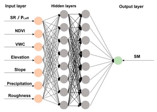
Figure 2.
The back-propagation artificial neural network (BP-ANN) model to estimate monthly SM.
In order to choose the optimal input variables for SM retrieval, contributions of individual variables and their combinations to the sensitivity of SM were assessed (using the correlation coefficient (R), RMSE, and the mean absolute error (MAE) as indicators), as shown in Table 4. The statistical indices from models 2 and 3 show that the combination of NDVI and VWC provides an optimal performance. Models 3~5 show that elevation and precipitation appear to positively affect the model, and precipitation has a slightly lower impact than that of elevation. Models 6 and 7 were used to investigate the slope and surface roughness, and both show positive correlations with SM. The contribution of noise is negative, as shown in models 8 and 9, so this variable is not selected. Most important of all, to determine the contribution of SR, model 10 used all the other variables (excluding noise) except SR. Note that the correlation coefficient of model 10 is much lower than that of other models, which proves that the SR has the highest impact on the overall performance. The best variable combination (i.e., model 7) was selected for the subsequent SM estimation. The model test was executed using CYGNSS data from April 2018.
Table 4.
Variables used to fit the SM.
Three different layers were contained in the model, i.e., the input layer, the hidden layer, and the output layer. The input layer contained multi-parameters affecting SM, i.e., NDVI, vegetation water content (VWC), elevation, slope, precipitation, and roughness data, as shown in Figure 2. The NDVI and VWC were estimated from the Moderate-Resolution Imaging Spectroradiometer (MODIS) Aqua Surface Reflectance Daily Global 500 m data set. The elevation, slope and roughness data were derived from the SRTM 90 m DEM data set. The precipitation was derived from the Global Precipitation Measurement (GPM) Level 3 data set. The SMAP Level 3 SM data with a 9-km resolution were used in the output layer during the training stage of the model for optimization of the BP-ANN parameters. All data sets of the input and output layers were averaged to obtain monthly values. The VWC and roughness were computed from NDVI and slope with empirical relations [39,40], respectively.
The datasets were normalized to obtain values between 0 and 1 prior to training. The datasets were divided into a training set, testing set, and validation set, accounting for 60%, 20%, and 20%, respectively. The training set was used to adjust the weights on the neural network, the testing set was used to test the network performance, and the validation set was used to minimize overfitting [34,36]. Repeated trainings were tested to obtain an optimal neural network to achieve reasonable results. Table 5 shows the accuracy assessment of the multiple regression models. As shown in Table 5, the non-linear model is better than the corresponding linear model; two hidden layers show the highest precision; also, the hyperbolic tangent performs better than others. Hence, the ANN structure used in this paper was as follows: the input layer has seven nodes, which is the same as the number of used features. The output layer has a single node that is the predicted SM values. There are two hidden layers, and the number of nodes is 8. The hyperbolic tangent is chosen as the activation function. The last layer is a regression layer with no activation function. The maximum training number was set to 6000, the error metric was being minimized as RMSE, the error threshold was set to 0.001, and the learning rate was set to 0.05.
Table 5.
Accuracy assessment of the BP-ANN structures.
3. Results and Comparisons
In this section, the results of TDS-1 and CYGNSS were analyzed for sensitivity analysis on a daily basis and SM estimation on a monthly basis, respectively. Due to the fact that the TDS-1 data stopped transmitting data in December 2018, and the data after April 2018 is very sparse, in Section 3.1 and Section 3.2, data from the overlapping time period (between May 2017 and April 2018) of the two satellite missions were used for evaluation. In Section 3.3, to match up with the one-year’s in situ measurements collected from April 2018 to May 2019, the TDS-1 derived SM in April 2018 were compared with in situ measurements, and the CYGNSS derived SMs from April 2018 to May 2019 were compared with in situ measurements.
For the daily results, since the TDS-1 data are distributed discretely and the daily MODIS NDVI data set is severely affected by cloud and fog, SR and Pr,eff are used as a proxy to compare with the SMAP SM dataset. For monthly results, the BP-ANN method proposed in Section 2.4 was used to estimate SM. All input parameters for the model (including TDS-1 Pr,eff and CYGNSS SR) were monthly averaged. Note that the monthly SM were derived in a separate way and were not simply inherited from the daily results. The temporal behavior of estimated SM, SMAP SM, and in situ measurements were examined during the entire period. Three statistical indices, i.e., ubRMSE, MAE, and R, were computed to quantify the accuracy.
3.1. Sensitivity Analysis from TDS-1 and CYGNSS on a Daily Basis
As an example, Figure 3a,b show the Pr,eff distribution of TDS-1, and SR distributions of TDS-1 and CYGNSS in May 2017, respectively. Overall, neither data sets are available for the southwestern portion of Mainland China; the TDS-1 covers northern China. The distribution of the TDS-1 results is more discrete than those of CYGNSS, and there are only seven months of TDS-1 data available within the observed period. Additionally, the longer revisiting time (10~35 days) of the TDS-1 payload compared to that of CYGNSS (2.8~7 h) also leads to this phenomenon. In addition, compared to TDS-1, the SR derived from CYGNSS exhibits a slightly higher correlation with the SMAP SM (R = 0.561 vs. R = 0.613).
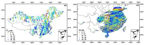
Figure 3.
(a) Distribution of TDS-1 Pr,eff in May 2017; (b) distribution of CYGNSS SR in May 2017.
Due to the sparse distribution of TDS-1, for each grid cell (9 × 9-km), the maximum number of matches of TDS-1 Pr,eff and SMAP SM is 11; most are five to seven, so the R estimation for each grid may not be very particularly accurate. Thus, only the R of the SR derived from CYGNSS against the SMAP SM for each grid cell over the entire time period is shown (Figure 4a). The inner box in Figure 4a illustrates the numerical distributions of R for CYGNSS at a daily scale. The VWC estimated from NDVI with empirical relations [39] is also presented to show the influence of vegetation on the derived SM (Figure 4b). Overall, the performance of the SM derived from CYGNSS shows different consistency with the SMAP SM. The low R values mainly occur in the central regions where the VWC values are obviously high, and the high R values occur in the northeast and south where the VWC values are relatively low. This indicates that the SR derived from CYGNSS could not guarantee an absolutely high accuracy of the SM estimates when the VWC is high, which is consistent with previous studies [8,25]. This may be due to the absorption of the signal by the vegetation resulting in a large attenuation of the signal intensity; thus, the estimated SM is lower than the actual value [24]. To estimate SM under dense vegetation, future research of an algorithm suitable for bare soil or low-vegetation surfaces should be improved to consider removing the effects of vegetation.
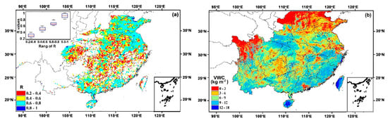
Figure 4.
(a) R between daily averaged CYGNSS SR and SMAP SM, (b) the averaged VWC estimated from NDVI with empirical relations over the observed time
Figure 5 shows the variations of CYGNSS, and TDS-1 against SMAP during the observation period at one specific grid (31.5°E, 104.4°N). This grid was selected because it contained the most CYGNSS data during the observed time. The SMAP SM data were interpolated to show a visually continuous curve in Figure 5; this does not affect the final accuracy. Note that the Pr,eff derived from TDS-1 and the SR derived from CYGNSS show good agreement with SMAP SM data (R = 0.682 for TDS-1, and R = 0.763 for CYGNSS). It should be pointed out that, due to the limited amount of TDS-1 data used, the comparison between TDS-1 and SMAP is almost not significant from a statistical point of view. For CYGNSS, the magnitudes are not always proportional to the SMAP SM when the SM is low (see the box in Figure 5). The underestimates of the SMAP SM products over high vegetation regions may lead to this phenomenon [41,42]. The difference in scales between the SMAP pixels and the CYGNSS points may also be linked to the biases.
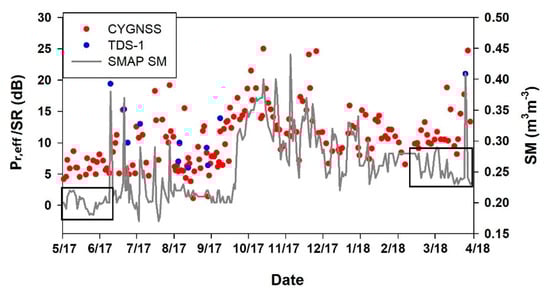
Figure 5.
Variations of CYGNSS, TDS-1, and SMAP during the observation period.
3.2. SM Estimation From TDS-1 and CYGNSS on a Monthly Basis
Compared with most atmospheric processes, soil moisture has a longer memory time and may impact the climatic characteristics; hence, monthly SM is a key variable for climatology studies and soil hydrology [37,38].
The BP-ANN model proposed in Section 2.4 was used to estimate SM on a monthly basis. For TDS-1, one-year data (from May 2016 to April 2017) of TDS-1 were used to train the model, and for CYGNSS, one-year data (from April 2018 to March 2019) were used to train the model. For both TDS-1 and CYGNSS, one-year data over the two missions’ overlapping time period (i.e., between May 2017 and April 2018) were used to predict the monthly SM. Taking advantage of the predicted SM over the entire overlapping time period, the main purpose of this section was to compare the performance of CYGNSS SM with SMAP SM on a monthly basis, and in the meantime, to cross-validate the BP-ANN model using the SMAP SM data from a relatively independent time period. The following results shown in this section are all based on the predicted SM over the overlapping time period. To make the analysis consistent, all the results were converted to gridded data. The CYGNSS data were gridded to 10-km. Considering the sparse distribution of TDS-1 in Mainland China, 50 km was applied for TDS-1; thus, it cannot present as much detailed SM information as CYGNSS. The data value per grid cell was determined to be the mean value of the specular points in the grid.
The data from one month of each season were chosen to display the results. Because there were only seven months of TDS-1 data available within the observed period, the selected months (i.e., June, November, February, and April) were not evenly time spaced. Figure 6 shows spatial comparisons of the SM derived from TDS-1 with the SMAP SM. Generally, the SM derived from TDS-1 shows good agreement with the SMAP SM. The central region of Mainland China shows a high SM value during the observation period (the green box in Figure 6a1), which is consistent with the variations of SMAP SM. In addition, SM in the north region shows little variation (the blue box in Figure 6a1); conversely, the SM in the tropic region (the gray box in Figure 6a1) tends to be high most of the time.
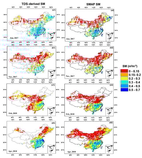
Figure 6.
Comparisons of the SM derived from TDS-1 and the SMAP SM. (a1–a2) June 2017, (b1–b2) November 2017, (c1–c2) February 2018, and (d1–d2) April 2018.
Figure 7 shows the variations of the SM derived from CYGNSS and the SMAP SM over Mainland China during the same four months as that of TDS-1 in Figure 6. Overall, the CYGNSS data well reflects the SM dynamics during the observed period with different seasonal amplitudes, and there is a good agreement between CYGNSS and SMAP. Spatially, the estimated SM varies significantly, similar to that of TDS-1 in Figure 6. Note that the estimated SM of the northeast (the box in Figure 7a1) shows lower variation compared with other areas, and the SM maintains a constant value of around < 0.4 m3m−3 during the full year. This is consistent with SMAP SM. The SM in central and southern Mainland China show variations between locations.
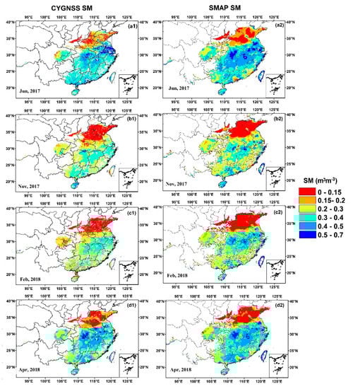
Figure 7.
Comparisons of the SM derived from CYGNSS and the SMAP SM. (a1–a2) June 2017, (b1–b2) November 2017, (c1–c2) February 2017, and (d1–d2) April 2018.
Figure 8 shows the spatial patterns of R, ubRMSE, and MAE of the TDS-1 and CYGNSS against SMAP on a monthly basis, respectively. Generally, CYGNSS performs well with good spatial patterns for all three indices, indicating that CYGNSS data could be used to produce an SM product (R = 0.798; ubRMSE = 0.062 m3m−3; MAE = 0.040 m3m−3); TDS-1 also shows good results, but with sparse spatial distribution (R = 0.676; ubRMSE = 0.052 m3m−3; MAE = 0.060 m3m−3).
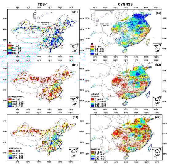
Figure 8.
Statistical indices for the SM derived from TDS-1/CYGNSS against the SMAP SM. (a1–a2) R, (b1–b2) ubRMSE, and (c1–c2) MAE.
The inner boxes in Figure 8a1,a2 illustrate the numerical distributions of R for TDS-1 and CYGNSS, respectively. As shown in Figure 8a1, for TDS-1, over 65% of the R values are higher than 0.4, and the ubRMSE values are smaller than 0.08 m3m−3 over most areas, while those values are larger than 0.08 m3m−3 in the northeast. For the MAE of TDS-1, the values are smaller than 0.07 m3m−3 in most parts of Mainland China, while they are larger than 0.07 m3m−3 in the northeast, which is similar to the case of the ubRMSE. Additionally, because overlapping TDS-1 data were used for both monthly SM and daily SM sensitivity analysis (May 2016 through April 2017), the proposed model exhibits a higher correlation with the SMAP SM than that of Pr,eff compared to the daily results (R = 0.561 vs. R = 0.676). In terms of CYGNSS, the R values are higher in the north and, conversely, tend to be lower in the central area. Incoherent scattering due to volume scattering from dense vegetation and large surface roughness could be the possible reason for this phenomenon. Regarding the distributions of ubRMSE, the values are generally lower than 0.08 m3m−3 over 50% of Mainland China, which is similar to the TDS-1 results. In part of the central regions, the ubRMSE values are rarely larger than 0.08 m3m−3, which are similar to the R distributions and are consistent with that of TDS-1. The MAE values are less than 0.03 m3m−3 over most of Mainland China.
The average values of the three statistical indices per month basis are shown in Figure 9. For TDS-1 (Figure 9a), the ubRMSE and MAE values are less than 0.075 m3m−3 and 0.08 m3m−3 over the entire time period, respectively, and the values of the two indices both show increasing trends from May to October, which are relevant to the declining trend of the R. As shown in Figure 9b, the CYGNSS R are higher than 0.7 in most months and, conversely, tend to be low from August to October. Similar to TDS-1, the CYGNSS MAE value shows a rising trend from June to September, which indicates that the estimated SM had lower accuracies from June to September compared to other months. This is probably due to the growth of vegetation and the increase in surface roughness. The histograms of sample numbers were also shown. The sample numbers of CYGNSS show little differences per month. However, the sample numbers of TDS-1 vary from month to month. For example, the numbers of TDS-1 in July and October 2017 are very few, which may due to the instability of the payload. This may lead to the precision of SM estimates in these two months lower than other months.
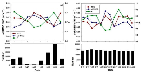
Figure 9.
Comparisons of the three statistical indices (i.e., ubRMSE, MAE, and R) between TDS-1/CYGNSS and SMAP. (a) TDS-1 vs. SMAP, (b) CYGNSS vs. SMAP.
3.3. Validation of TDS-1 and CYGNSS Results with in Situ Measurements
Given the limitations of the model construction and the cross-validation (i.e., the dependence of SMAP data during the training and predicting stages of the model) described in the Section 2.4 and Section 3.2, the in situ measurements derived from dense SM ground networks of Mainland China were introduced to further validate the model results. The TDS-1 data and in situ measurements only overlapped in April 2018, and the TDS-1 SM results from longitude 95.9° to 130° were selected for validation. As shown in Figure 10, the SM derived from TDS-1 shows a good correlation with the in situ data (R = 0.687, ubRMSE = 0.056 m3m−3, MAE = 0.066 m3m−3). Note that higher SM is observed in wetland and riverine areas (longitudes between 110° to 118°). Meanwhile, in the north areas (longitudes between 120° to 129.8°), the SM values tend to be lower, which is consistent with the climate features of China.
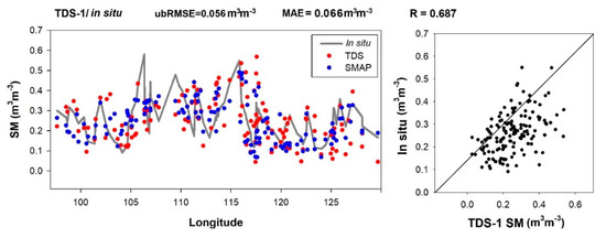
Figure 10.
Correlations of the SM derived from TDS-1, SMAP SM, and in situ measurements for locations with longitudes between 95.9° to 129.8° in April 2018.
The statistical indices of each month between the SM derived from CYGNSS, and the in situ measurements are displayed in Figure 11. The indices illustrate that the variability of the SM derived from CYGNSS is in good agreement with that of the in situ measurements (averaged R = 0.724, averaged ubRMSE = 0.053 m3m−3, averaged MAE = 0.052 m3m−3). It is particularly noteworthy that, similar to Figure 8b, between May and October, the Rs tend to be lower, and the ubRMSE and MAE values tend to be larger than those of other months.
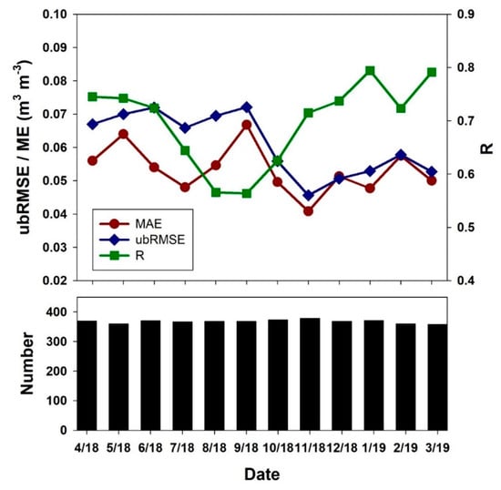
Figure 11.
Comparisons of ubRMSE, MAE, and R between the SM derived from CYGNSS and the in situ measurements.
Three typical regions (i.e., Shandong (the blue box in Figure 12d), Jiangxi (the green box in Figure 12d)), and Guangdong Province (the gray box in Figure 12d) represent different climate conditions and vegetation densities and thus were chosen to further analyze the temporal variations of the estimated SM (Figure 12a–c). Figure 12a–c shows the time-series at each site. Twenty-seven sites in each typical region were chosen. Since the in situ data were monthly averaged, so 12 points were contained for each site per year, representing twelve months. Figure 12a shows sites distributed in a tropic region, i.e., Guangdong Province. The NDVI at this location varies from 0 to 0.6. There were high SM values associated with the tropical climate. Fluctuations in the SM derived from CYGNSS are similar to the SMAP SM and in situ measurements across the entire observation time and exhibit the highest correlation (R = 0.856). Figure 12b shows sites distributed in a subtropical monsoon climate region, i.e., Jiangxi Province. Note that CYGNSS, SMAP and ground observations show large variations, with the lowest correlation (R = 0.672). Compared with the other two cases, these sites were influenced by vegetation cover more seriously with higher NDVI values (0 to 0.7). As shown in Figure 12c, the Shandong Province is under a temperate monsoon climate condition, and the average NDVI varies between 0 and 0.5. All SM derived from CYGNSS, SMAP SM, and in situ measurements show little variations. The correlation value (R = 0.758) is relatively higher than that in Figure 12b, whereas CYGNSS continues to provide an underestimate with a small negative bias value over the entire time period (MAE = 0.057 m3m−3).
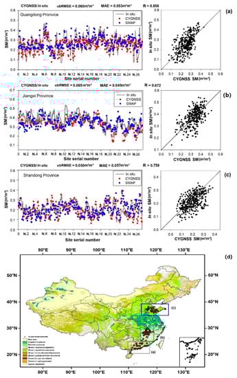
Figure 12.
Correlations of the SM derived from CYGNSS, SMAP SM, and in situ measurements for three provinces with typical climate conditions, (a) Guangdong Province, (b) Jiangxi Province, (c) Shandong Province, (d) the sites distribution.
4. Discussion
4.1. Issues Related to the BP-ANN Model
Overall, the proposed model based on BP-ANN generated promising results with comparable accuracy to the referenced SMAP data and the in situ measurements, demonstrating that it could be generalized for regional SM estimation. However, because the SMAP SM data were used in the output layer of the BP-CNN model during the training stage, the correlation coefficients of the estimated SM and the SMAP SM (R = 0.676 for TDS-1; R = 0.798 for CYGNSS) were similar with or better than that of the estimated SM and the in situ measurements (R = 0.687 for TDS-1; R = 0.724 for CYGNSS). Although similar validation methods have been used in other publications [12,24], it is better to involve other data sources to cross-validate the SM results.
The model can be further trained with additional variables affecting SM (e.g., vegetation optical depth and soil composition). It should also be noted that an increase in parameters does not always improve accuracy. Additionally, the proposed model in this study was not applicable for a daily scale. Future research should consider this issue and improve the model by involving additional daily ancillary data from multiple sources.
4.2. Advantages and Limitations of Spaceborne GNSS-R for Estimating SM
Spaceborne GNSS-R, e.g., TDS-1 and CYGNSS as presented in this study, can estimate SM with accuracy comparable to L band SM satellite missions such as SMAP. The results show the two mission can estimate SM with accuracy comparable to L band SM satellite missions such as SMAP. Moreover, as the first GNSS-R constellation, CYGNSS can provide detailed spatial variabilities of SM with a very short revisit time. The GNSS-R payload is light in weight and cost effective, which makes it possible to design small satellite constellations. It is believed that future spaceborne GNSS-R missions will have better spatial and temporal resolutions for sensing SM.
Possible errors of estimating SM using TDS-1/CYGNSS are explained as follows:
- Different spatial scales between in situ/SMAP points and TDS-1/CYGNSS points. Although ground measurements from dense sites were used to reduce this well-known issue, the differences in spatial resolution continue to introduce deviations. Future research may consider downscaling the SMAP SM product to the same resolution as the GNSS-R.
- Effects in terms of VWC, roughness, and elevation etc. For daily sensitivity analysis results, the vegetation severely affects the accuracy of SM, particularly over the central part of Mainland China (VWC > 6 kg/m2 vs. R < 0.6). The accuracies of monthly results were improved since these variables were considered in the proposed neural network model. Nevertheless, surface roughness and complex terrain environments may still reduce the estimation accuracy. Subsequent research may attempt to a potential way to reduce this impact by using changes instead of absolute reflectivity values.
- Mismatch between the depth of microwave penetration and the depth of in situ SM measurements. The in situ measurements used for validation are at 10 cm, whilst the GNSS L-band signal has various penetration depths between 0 cm and 20 cm, depending on the soil’s wetness, as Camp et al. shown in [8].
- Difficulty of matching different remote sensing datasets to each other and the GNSS-R daily values. As mentioned before, the daily MODIS NDVI data set is severely affected by cloud and fog, and currently NDVI does not have a commonly used product. Future study may focus on generation of daily continuous surface soil moisture of high spatial resolution using spaceborne GNSS-R data; daily NDVI estimation method as Zhao et al. proposed [43] may be a good inspiration.
5. Conclusions
This study, taking Mainland China as an example, gave a comprehensive evaluation and comparison of using TDS-1 and CYGNSS data sets to estimate SM. For sensitivity analysis on a daily basis, the two data were matched up regionally and compared over the overlapping periods (May 2017–April 2018) with SMAP SM. For SM estimation on a monthly basis, an algorithm based on BP ANN was proposed to estimated SM. The algorithm combined variables (e.g., vegetation cover, surface roughness, elevation, and precipitation) that highly related to SM estimation. The predicted SM showed strong and positive linear relationship with SMAP SM and in situ measurements, respectively. The findings of this study suggested that TDS-1/CYGNSS and upcoming spaceborne GNSS-R missions could be new and powerful data sources to produce SM data sets at large scale and with relatively high precision.
Author Contributions
Conceptualization, T.Y., W.W., Z.S., and X.C.; methodology, T.Y. and W.W.; validation, T.Y.; formal analysis T.Y. and B.L.; resources, S.L.; writing—original draft preparation, T.Y.; writing—review and editing, T.Y., W.W., and Z.S.; supervision, Z.S. and X.C.; funding acquisition, Z.S., W.W., and S.L. All authors have read and agreed to the published version of the manuscript.
Funding
This work was jointly supported by the National Natural Science Foundation of China (Grant No. 41971377, 41501360), the Strategic Priority Research Program of the Chinese Academy of Sciences (Grant Nos. XDA23050102, XDA19040303), and the National Key Research and Development Program of China (Grant Nos. 2017YFC0503805, 2017YFD0300101).
Acknowledgments
The authors would like to thank the China Meteorological Administration (CMA) for providing in situ SM data. The authors would also like to thank the TDS-1, CYGNSS, and SMAP scientific teams for their hard work in providing the data used in this study.
Conflicts of Interest
The authors declare no conflict of interest.
References
- Rodriguez-Alvarez, N.; Camps, A.; Vall-Llossera, M.; Bosch-Lluis, X.; Monerris, A.; Ramos-Perez, I.; Valencia, E.; Marchan-Hernandez, J.F.; Martinez-Fernandez, J.; Baroncini-Turricchia, G.; et al. Land geophysical parameters retrieval using the interference pattern GNSS-R technique. IEEE Trans. Geosci. Remote 2010, 49, 71–84. [Google Scholar] [CrossRef]
- Cardellach, E.; Rius, A.; Martín-Neira, M.; Fabra, F.; Nogués-Correig, O.; Ribó, S.; D’Addio, S. Consolidating the precision of interferometric GNSS-R ocean altimetry using airborne experimental data. IEEE Trans. Geosci. Remote 2013, 52, 4992–5004. [Google Scholar] [CrossRef]
- Clarizia, M.P.; Gommenginger, C.P.; Gleason, S.T.; Srokosz, M.A.; Galdi, C.; Di Bisceglie, M. Analysis of GNSS-R delay-Doppler maps from the UK-DMC satellite over the ocean. Geophys. Res. Lett. 2009, 36, 2. [Google Scholar] [CrossRef]
- Clarizia, M.P.; Gommenginger, C.; Di Bisceglie, M.; Galdi, C.; Srokosz, M.A. Simulation of L-band bistatic returns from the ocean surface: A facet approach with application to ocean GNSS reflectometry. IEEE Trans. Geosci. 2011, 50, 960–971. [Google Scholar] [CrossRef]
- Foti, G.; Gommenginger, C.; Jales, P.; Unwin, M.; Shaw, A.; Robertson, C.; Rosello, J. Spaceborne GNSS reflectometry for ocean winds: First results from the UK TechDemoSat-1 mission. Geophys. Res. Lett. 2015, 42, 5435–5441. [Google Scholar] [CrossRef]
- Chew, C.; Shah, R.; Zuffada, C.; Hajj, G.; Masters, D.; Mannucci, A.J. Demonstrating soil moisture remote sensing with observations from the UK TechDemoSat-1 satellite mission. Geophys. Res. Lett. 2016, 43, 3317–3324. [Google Scholar] [CrossRef]
- Alonso-Arroyo, A.; Zavorotny, V.U.; Camps, A. Sea ice detection using UK TDS-1 GNSS-R data. IEEE Trans. Geosci. Remote 2017, 55, 4989–5001. [Google Scholar] [CrossRef]
- Camps, A.; Park, H.; Pablos, M.; Foti, G.; Gommenginger, C.P.; Liu, P.W.; Judge, J. Sensitivity of GNSS-R spaceborne observations to soil moisture and vegetation. IEEE J-STARS 2016, 9, 4730–4742. [Google Scholar] [CrossRef]
- Di Simone, A.; Park, H.; Riccio, D.; Camps, A. Sea target detection using spaceborne GNSS-R delay-Doppler maps: Theory and experimental proof of concept using TDS-1 data. IEEE J-STARS 2017, 10, 4237–4255. [Google Scholar] [CrossRef]
- Clarizia, M.P.; Ruf, C.S. Wind speed retrieval algorithm for the Cyclone Global Navigation Satellite System (CYGNSS) mission. IEEE Trans. Geosci. Remote 2016, 54, 4419–4432. [Google Scholar] [CrossRef]
- Chew, C.; Reager, J.T.; Small, E. CYGNSS data map flood inundation during the 2017 Atlantic hurricane season. Sci. Rep. 2018, 8, 1–8. [Google Scholar] [CrossRef] [PubMed]
- Chew, C.C.; Small, E.E. Soil Moisture Sensing Using Spaceborne GNSS Reflections: Comparison of CYGNSS Reflectivity to SMAP Soil Moisture. Geophys. Res. Lett. 2018, 45, 4049–4057. [Google Scholar] [CrossRef]
- Wan, W.; Liu, B.; Zeng, Z.; Chen, X.; Wu, G.; Xu, L.; Chen, X.; Hong, Y. Using CYGNSS data to monitor China’s flood inundation during typhoon and extreme precipitation events in 2017. Remote Sens. 2019, 11, 854. [Google Scholar] [CrossRef]
- Unwin, M.; Jales, P.; Tye, J.; Gommenginger, C.; Foti, G.; Rosello, J. Spaceborne gnss-reflectometry on techdemosat-1: Early mission operations and exploitation. IEEE J-STARS 2018, 9, 4525–4539. [Google Scholar] [CrossRef]
- Eroglu, O.; Kurum, M.; Boyd, D.; Gurbuz, A.C. High spatio-temporal resolution CYGNSS soil moisture estimates using artificial neural networks. Remote Sens. 2019, 11, 2272. [Google Scholar] [CrossRef]
- Owe, M.; de Jeu, R.; Walker, J. A methodology for surface soil moisture and vegetation optical depth retrieval using the microwave polarization difference index. IEEE Trans. Geosci. Remote 2001, 39, 1643–1654. [Google Scholar] [CrossRef]
- Rahimzadeh-Bajgiran, P.; Berg, A.A.; Champagne, C.; Omasa, K. Estimation of soil moisture using optical/thermal infrared remote sensing in the Canadian Prairies. ISPRS J. Photogramm. 2013, 83, 94–103. [Google Scholar] [CrossRef]
- Brocca, L.; Ciabatta, L.; Massari, C.; Camici, S.; Tarpanelli, A. Soil moisture for hydrological applications: Open questions and new opportunities. Water 2017, 9, 140. [Google Scholar] [CrossRef]
- Draper, C.S.; Reichle, R.H.; De Lannoy, G.J.M.; Liu, Q. Assimilation of passive and active microwave soil moisture retrievals. Geophys. Res. Lett. 2012, 39. [Google Scholar] [CrossRef]
- Portal, G.; Vall-Llossera, M.; Piles, M.; Camps, A.; Chaparro, D.; Pablos, M.; Rossato, L. A spatially consistent downscaling approach for SMOS using an adaptive moving window. IEEE J-STARS 2018, 11, 1883–1894. [Google Scholar] [CrossRef]
- Camps, A. Spatial resolution in GNSS-R under coherent scattering. IEEE Geosci. Remote Sens. 2019, 17, 32–36. [Google Scholar] [CrossRef]
- Entekhabi, D.; Njoku, E.G.; O’Neill, P.E.; Kellogg, K.H.; Crow, W.T.; Edelstein, W.N.; Entin, J.K.; Goodman, S.D.; Jackson, T.J.; Johnson, J.; et al. The soil moisture active passive (SMAP) mission. Proc. IEEE 2010, 98, 704–716. [Google Scholar] [CrossRef]
- Kerr, Y.H.; Waldteufel, P.; Wigneron, J.P.; Martinuzzi, J.A.M.J.; Font, J.; Berger, M. Soil moisture retrieval from space: The Soil Moisture and Ocean Salinity (SMOS) mission. IEEE Trans. Geosci. Remote 2001, 39, 1729–1735. [Google Scholar] [CrossRef]
- Kim, H.; Lakshmi, V. Use of Cyclone Global Navigation Satellite System (CYGNSS) observations for estimation of soil moisture. Geophys. Res. Lett. 2018, 45, 8272–8282. [Google Scholar] [CrossRef]
- Camps, A.; Park, H.; Portal, G.; Rossato, L. Sensitivity of TDS-1 GNSS-R reflectivity to soil moisture: Global and regional differences and impact of different spatial scales. Remote Sens. 2018, 10, 1856. [Google Scholar] [CrossRef]
- Carreno-Luengo, H.; Amèzaga, A.; Vidal, D.; Olivé, R.; Munoz, J.F.; Camps, A. First polarimetric GNSS-R measurements from a stratospheric flight over boreal forests. Remote Sens. 2015, 7, 13120–13138. [Google Scholar] [CrossRef]
- De Roo, R.D.; Ulaby, F.T. Bistatic specular scattering from rough dielectric surfaces. IEEE Trans. Antennas Propag. 1994, 42, 220–231. [Google Scholar] [CrossRef]
- Carreno-Luengo, H.; Luzi, G.; Crosetto, M. Effects of rough topography in GNSS-R: A parametric study based on a digital elevation model. In Proceedings of the IGARSS 2019—2019 IEEE International Geoscience and Remote Sensing Symposium, Yokohama, Japan, 28 July–2 August 2019; pp. 8663–8666. [Google Scholar]
- Carreno-Luengo, H.; Luzi, G.; Crosetto, M. Impact of the elevation angle on cygnss gnss-r reflectivity over different scattering media over land and ocean. In Proceedings of the IGARSS 2018—2018 IEEE International Geoscience and Remote Sensing Symposium, Valencia, Spain, 22–27 July 2018; pp. 1051–1054. [Google Scholar]
- Carreno-Luengo, H.; Luzi, G.; Crosetto, M. Biomass estimation over tropical rainforests using GNSS-R on-board the CyGNSS microsatellites constellation. In Proceedings of the IGARSS 2019—2019 IEEE International Geoscience and Remote Sensing Symposium, Yokohama, Japan, 28 July–2 August 2019; pp. 8676–8679. [Google Scholar]
- Carreno-Luengo, H.; Camps, A.; Querol, J.; Forte, G. First results of a GNSS-R experiment from a stratospheric balloon over boreal forests. IEEE Trans. Geosci. Remote 2015, 54, 2652–2663. [Google Scholar] [CrossRef]
- Feng, Y.; Zhang, W.; Sun, D.; Zhang, L. Ozone concentration forecast method based on genetic algorithm optimized back propagation neural networks and support vector machine data classification. Atmos. Environ. 2011, 45, 1979–1985. [Google Scholar] [CrossRef]
- Specht, D.F. A general regression neural network. IEEE Trans. Neural Netw. 1991, 2, 568–576. [Google Scholar] [CrossRef]
- Cui, Y.; Long, D.; Hong, Y.; Zeng, C.; Zhou, J.; Han, Z.; Liu, R.; Wan, W. Validation and reconstruction of FY-3B/MWRI soil moisture using an artificial neural network based on reconstructed MODIS optical products over the Tibetan Plateau. J. Hydrol. 2016, 543, 242–254. [Google Scholar] [CrossRef]
- Wang, J.; Ji, H.; Wang, Q.G.; Li, H.; Qian, X.; Li, F.; Yang, M. Prediction of size-fractionated airborne particle-bound metals using MLR, BP-ANN and SVM analyses. Chemosphere 2017, 180, 513–522. [Google Scholar]
- Yang, S.; Feng, Q.; Liang, T.; Liu, B.; Zhang, W.; Xie, H. Modeling grassland above-ground biomass based on artificial neural network and remote sensing in the Three-River Headwaters Region. Remote Sens. Environ. 2018, 204, 448–455. [Google Scholar] [CrossRef]
- Fan, Y.; Van Den Dool, H. Climate Prediction Center global monthly soil moisture data set at 0.5 resolution for 1948 to present. J. Geophys. Res. Atmos. 2004, 109. [Google Scholar] [CrossRef]
- Wu, W.; Geller, M.A.; Dickinson, R.E. The response of soil moisture to long-term variability of precipitation. J. Hydrometeorol. 2002, 3, 604–613. [Google Scholar] [CrossRef]
- Jackson, T.J.; Le Vine, D.M.; Hsu, A.Y.; Oldak, A.; Starks, P.J.; Swift, C.T.; Isham, J.D.; Haken, M. Soil moisture mapping at regional scales using microwave radiometry: The Southern Great Plains Hydrology Experiment. IEEE Trans. Geosci. Remote 1999, 37, 2136–2151. [Google Scholar] [CrossRef]
- Campbell, S.; Simmons, R.; Rickson, J.; Waine, T.; Simms, D. Using Near-Surface Photogrammetry Assessment of Surface Roughness (NSPAS) to assess the effectiveness of erosion control treatments applied to slope forming materials from a mine site in West Africa. Geomorphology 2018, 322, 188–195. [Google Scholar] [CrossRef]
- Colliander, A.; Jackson, T.J.; Bindlish, R.; Chan, S.; Das, N.; Kim, S.B.; Asanuma, J. Validation of SMAP surface soil moisture products with core validation sites. Remote Sens. Environ. 2017, 191, 215–231. [Google Scholar] [CrossRef]
- Ma, C.; Li, X.; Wei, L.; Wang, W. Multi-scale validation of smap soil moisture products over cold and arid regions in northwestern china using distributed ground observation data. Remote Sens. 2017, 9, 327. [Google Scholar] [CrossRef]
- Zhao, M.; Heinsch, F.A.; Nemani, R.R.; Running, S.W. Improvements of the MODIS terrestrial gross and net primary production global data set. Remote Sens. Environ. 2005, 95, 164–176. [Google Scholar] [CrossRef]
© 2020 by the authors. Licensee MDPI, Basel, Switzerland. This article is an open access article distributed under the terms and conditions of the Creative Commons Attribution (CC BY) license (http://creativecommons.org/licenses/by/4.0/).