Article

Uncertainty Analysis for RadCalNet Instrumented Test Sites Using the Baotou Sites BTCN and BSCN as Examples

1
Key Laboratory of Quantitative Remote Sensing Information Technology, Aerospace Information Research Institute, Chinese Academy of Sciences, Beijing 100094, China
2
Environment Department, National Physical Laboratory, Hampton Road, Teddington, Middlesex TW11 0LW, UK
3
Division of Optical Metrology, National Institute of Metrology, Beijing 100029, China
*
Author to whom correspondence should be addressed.
Remote Sens. 2020, 12(11), 1696; https://doi.org/10.3390/rs12111696
Submission received: 29 April 2020 / Revised: 22 May 2020 / Accepted: 24 May 2020 / Published: 26 May 2020

Abstract

:
Vicarious calibration and validation techniques are important tools to ensure the long-term stability and inter-sensor consistency of satellite sensors making observations in the solar-reflective spectral domain. Automated test sites, which have continuous in situ monitoring of both ground reflectance and atmospheric conditions, can greatly increase the match-up possibilities for a wide range of space agency and commercial sensors. The Baotou calibration and validation test site in China provides operational high-accuracy and high-stability vicarious calibration and validation for high spatial resolution solar-reflective remote-sensing sensors. Two sites, given the abbreviations BTCN (an artificial site) and BSCN (a natural sandy site), have been selected as reference sites for the Committee on Earth Observation Satellites radiometric calibration network (RadCalNet). RadCalNet requires sites to provide data in a consistent format but does not specify the required operational conditions for a RadCalNet site. The two Baotou sites are the only sites to date that make spectral measurements for their continuous operation. One of the core principles of RadCalNet is that each site should have a metrologically rigorous uncertainty budget which also describes the site’s traceability to the international system of units, the SI. This paper shows a formalized metrological approach to determining and documenting the uncertainty budget and traceability of a RadCalNet site. This approach follows the Guide to the Expression of Uncertainty in Measurement. The paper describes the uncertainty analysis for bottom-of-atmosphere and top-of-atmosphere reflectance in the spectral region from 400 to 1000 nm for the Baotou sites and gives preliminary results for the uncertainty propagating this to top-of-atmosphere reflectance.

Graphical Abstract

1. Introduction

Vicarious calibration methods—where satellite sensor observations are calibrated or monitored using ground observations of surface and atmospheric properties—have been used for radiometric satellite sensors operating in the solar-reflective spectral region (400–2500 nm) since the 1980s [1]. With the rapid growth in the number and variety of passive radiometric sensors operated by national and international space agencies and commercial operators, and with the growing range of applications, many of which require the combination of data from different satellite sensors or the establishment of long time series of data, such vicarious calibration methods have also become important to determine inter-sensor differences and to evaluate long-term stabilities.
Vicarious calibration sites are chosen to be radiometrically simple. Natural sand-based desert or pebbly areas are commonly used as these are spatially homogeneous, have dry, stable climates, rare cloud cover, and have a relatively flat spectral reflectance that can be easily interpolated between observations. Early vicarious calibration methods using ground observations were based on field campaigns where scientists measured such a site with handheld instruments at the same time as a satellite observation. Since the turn of the century, a small number of sites have operated automatic instruments to provide continuous data coverage (ROSAS [2] was established in 1997 at La Crau, France, and automated instruments were established in Railroad Valley Playa, USA, in 2002 [3]).
In recent years, the Working Group on Calibration and Validation of the Committee on Earth Observation Satellites (CEOS-WGCV) has worked to bring such sites into a single radiometric calibration network (RadCalNet) [4]. The aim of RadCalNet is to provide consistent top-of-atmosphere (TOA) reflectance products over several sites across the World to users through a common online portal [5] At the time of writing the portal has over 400 registered users across all continents. RadCalNet achieves consistency not by requiring a common measurement method (indeed there is a wide range of instrumentation and techniques) but through careful peer review of methodologies and analysis, through regular comparisons and quality assurance of site data, and by a common processor used to propagate from ground observations to TOA reflectance.
RadCalNet provides “fiducial reference measurements”. In this it follows the principles of the Quality Assurance Framework for Earth Observation (QA4EO [6]) that was ratified by CEOS in 2008. QA4EO is based around a core principle that “all EO data and derived products has associated with it a documented and fully traceable quality indicator” which provides sufficient information for users to judge the fitness-for-purpose of that data set for their application. It is therefore an essential component of RadCalNet that sites provide rigorous, peer-reviewed uncertainty budgets that are established from a systematic review of the full SI-traceability chain and following principles of “Earth Observation Metrology”.
In this paper we present a rigorous uncertainty analysis for the Baotou RadCalNet sites as an exemplar for how such uncertainty budgets should be considered. The paper is a collaboration between the operators of the Baotou sites (Aerospace Information Research Institute (AIR) in Chinese Academy of Sciences, formerly known as Academy of Opto-Electronics (AOE)) and two national metrology institutes (National Physical Laboratory (NPL) in the United Kingdom and National Institute of Metrology (NIM) in China). The uncertainty analysis here follows the Guide to the Expression of Uncertainty in Measurement (the GUM, [7]), a document that was formalized by the Joint Committee for Guides in Metrology, a consortium including the International Bureau of Weights and Measures (BIPM) and the international standards organizations (e.g., ISO).
Section 2 describes the Baotou sites. Section 3 explains the principles behind the uncertainty analysis and the traceability route for the Baotou sites and Section 4 describes the results of the uncertainty analysis.

2. The Baotou RadCalNet Sites

The Baotou Cal&Val site [8] (“Baotou site” in brief) is located at the Ming’an township, Urad Front Banner, Bayannur prefecture, Inner Mongolia Autonomous Region, China, about 50 km from Baotou city. There are two RadCalNet sites within the region, with BTCN at [40.8514°N, 109.6292°E] and BSCN at [40.8658°N, 109.6155°E]. The overall Baotou site extends over 35 km east-west and 16 km north-south, with total area 292.5 km2. It is about 1270 m above sea level. The surface of the surrounding area is mainly desert, bare land, grassland, and farmland. Baotou features a cold semi-arid climate with average annual precipitation of 300 mm.
The Baotou site is a comprehensive calibration test site with many different types of target for radiometric and geometric calibration and validation of both spectrally-reflective sensors and synthetic aperture radar (SAR) sensors. On the Baotou site there are four targets set up with permanent instrumentation to allow for continuous measurement of ground spectral reflectance (along with atmospheric parameters). Three of these targets are artificial targets, separately made of black, grey, and white gravel, and the fourth target is a natural target within a desert environment. The grey permanent artificial target was chosen to be one of the initial four RadCalNet sites in 2014 and the natural sandy site went through a formal process during 2019 and was accepted as a new RadCalNet site in 2020.

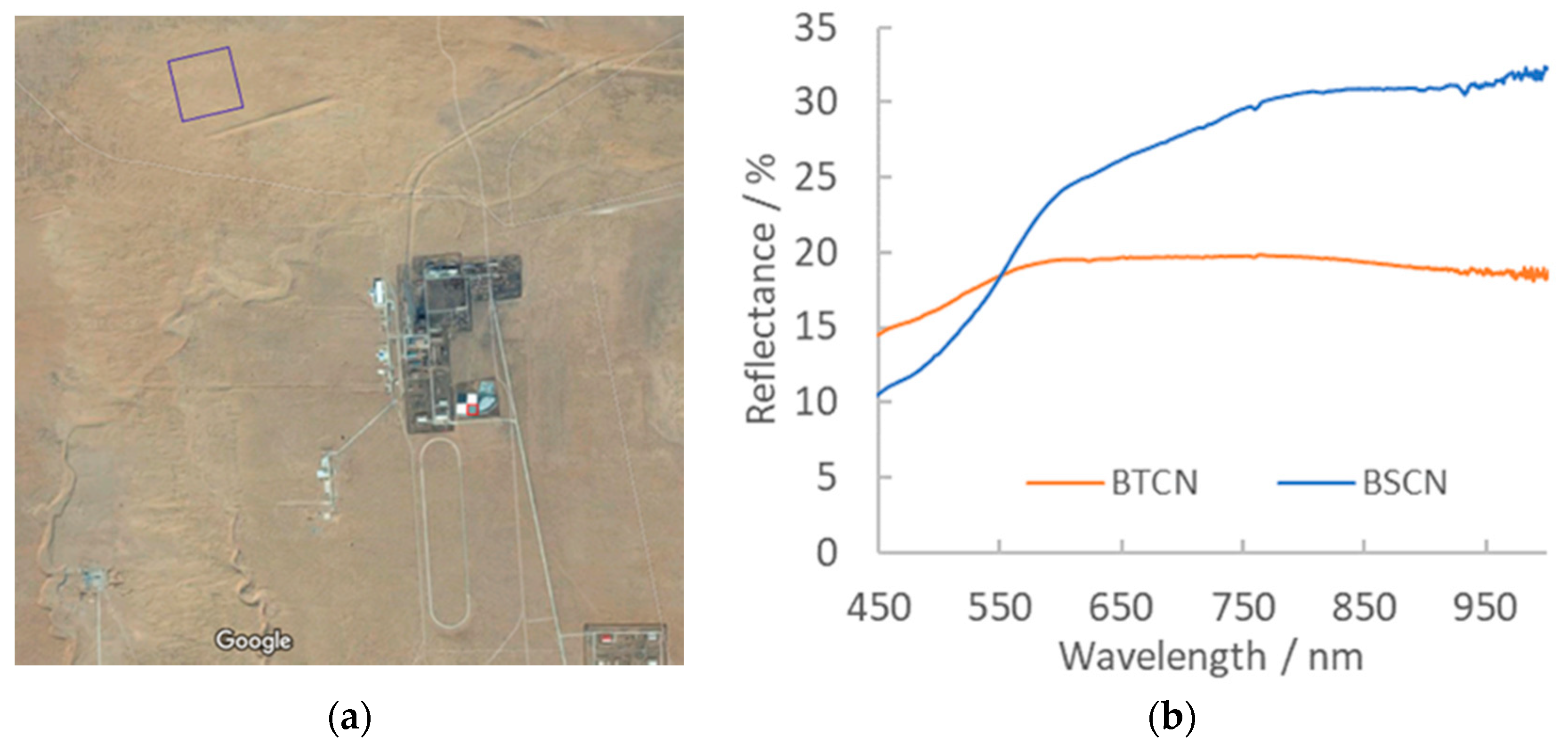
2.1. Grey Permanent Artificial Target and Sandy Site

To meet the requirements of wide dynamic range and stability of the ground targets in sensor radiometric calibration, multi-greyscale permanent artificial targets were built in the Baotou site. Figure 1 shows the image (from Google Earth) of the Baotou site area. In the permanent target region, the grey-scale artificial target is composed of two white, one grey, and one black uniform gravel squares, each of which covers an area of 48 × 48 m. The grey target has been incorporated into the RadCalNet as BTCN (marked by red squared box in Figure 1a) [8]. A sandy site (300 × 300 m), marked by blue squared box in Figure 1a) is 1.8 km away from the permanent target region to the north-west and was flattened in October 2015. The sandy site is a new RadCalNet site (BSCN). The typical spectral reflectances of the two sites are shown in Figure 1b, with reflectance approximately 20% (BTCN) and 30% (BSCN).

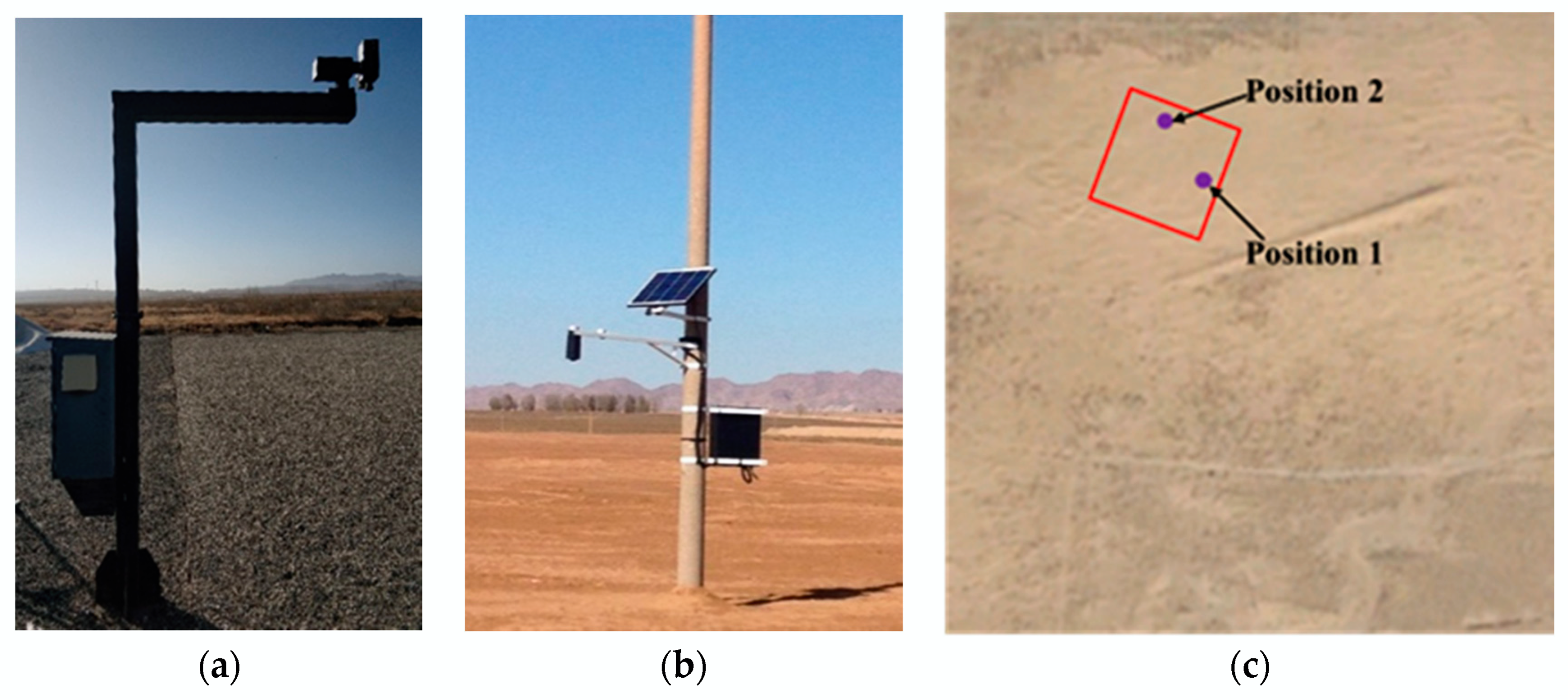
2.2. Site Instrumentation for RadCalNet

At the Baotou site, the surface-reflected radiance is measured by several automatic observation systems of ground-reflected radiance (one on the grey target and two on the sandy site) developed based on commercial Colorimetry Research (CR) series spectrometers produced by Colorimetry Research, Inc. The systems cover the spectral region from 380 to 1080 nm, with a spectral resolution (i.e., full width at half maximum, FWHM) of 2 nm, have nominally a 3° field of view and are mounted at a height of 2.5 m (BSCN) or 2.0 m (BTCN) (see Figure 2). They observe the ground at nadir every 2 min.
Aerosol and water vapor content atmospheric parameters are obtained from the AERONET [9] sun photometer that is near the BTCN grey target and 1800 m away from the BSCN sandy site. The sun photometer is a Cimel CE318 instrument operated by the Baotou Site operator and atmospheric data are available from the AERONET website [10]. An all-sky imager has been deployed at the Baotou site to acquire cloud amount, cloud picture, and cloud height.

3. Methods

3.1. A Metrological Approach

It is core to the RadCalNet philosophy that the sites are SI traceable and have uncertainty budgets determined in a metrologically-rigorous manner. The metrological approach is needed to ensure inter-site interoperability, to provide long-term stability, and to enable the sites to be compared with the satellite observations. Metrological traceability relies on three core principles: (1) an unbroken chain of calibrations back to the reference SI units, (2) the propagation of uncertainties through that chain, and (3) comparisons performed to validate uncertainty statements.
Here, we follow metrological best-practice with our analysis. The uncertainty analysis is performed according to the GUM [7] and its supplements, with the Law of Propagation of Uncertainties used to propagate uncertainties for the laboratory calibration and field operation of the instrument, and Monte Carlo Methods (GUM Supplement 1; [7]) providing uncertainties associated with the atmospheric radiative transfer.
As these sites operate continuously, we also need to consider the error correlation between different observations. The error is the unknown difference between the measured value and the conceptual true value. While this error is unknown, we can evaluate the associated uncertainty (the dispersion, around the measured value, of values that could reasonably be attributed to the measurand), and we can evaluate the error correlation, i.e., to what extent the unknown errors are common or independent between two observations. It is important to understand this to appropriately combine multiple observations. For RadCalNet data we need to consider error correlations between the two instruments on the BSCN site and between those and the instrument on the BTCN site, and also to understand the error correlation between multiple measurements by the same instrument. Finally, we need to consider error-correlation between the measured values in different spectrometer spectral channels.
Here we adapt a framework developed for documenting the uncertainty associated with satellite observations [11]. That approach, developed from metrological principles, involves the following steps: (1) We define the traceability chain and the measurement function for the observed measurand; (2) we present an “uncertainty tree diagram” that shows the effects (sources of uncertainty) that influence our measured value and how these propagate to the measured value; (3) for each effect we create an ‘effects table’ that documents the uncertainty, the error correlation structures on different dimensions, and the sensitivity coefficient (that translates the uncertainty associated with that effect into an uncertainty associated with the measurand), and (4) we provide a combined standard uncertainty associated with all effects, with independent effects (no error correlation), with common effects (full error correlation), and with structured effects (partial error correlation).
With the satellite sensors considered in [11], the error correlation structures were provided for within scanlines, between scanlines, and between orbits. Here we consider error correlation structures between observations of a single spectrometer, between spectrometers, and between wavelengths.

3.2. Traceability for Ground and Top-of-Atmosphere Reflectance

3.2.1. Principles of Radiative Transfer

To convert the observed radiance into reflectance, and to propagate reflectance to TOA, atmospheric radiative transfer must be considered. Figure 3 gives a simplified (ignoring multiple scattering) visualization of the relevant light paths. The red lines represent the illumination of the Baotou site. Some light illuminates the Baotou site directly from the sun. A proportion of this is lost through atmospheric scattering on the way to the site. The site is also illuminated by the sky through light that is scattered in the atmosphere onto the site (sky diffuse) and light which has reflected off nearby locations and scattered onto the site (sky scatter). We use the radiative transfer model MODTRAN-5 [12] to estimate both the direct solar irradiance (direct incoming beam minus the lost irradiance) and the sky irradiance (the combination of sky diffuse and sky scatter). When propagating to top of atmosphere we must consider light that reaches the satellite directly, the loss of radiation through scattering on the upward path and light that has scattered into the beam from the sun (without reaching the ground) or from other parts of the ground background. Again, MODTRAN-5 is used for this evaluation. Note that as a default MODTRAN-5 assumes that the surrounding ground has the same reflectance as the area of interest. Where this is not the case (e.g., for the grey site BTCN, which is an artificial target), there is an “adjacency effect” that must be separately considered (see Section 4.6).

3.2.2. Overview of Traceability

The observational spectrometers at the Baotou RadCalNet sites measure upwelling radiance from the surface. This upwelling radiance is converted to ground reflectance using the measurement equation:
ρ gnd ( θ , t ; λ i ) = π L gnd ( λ i , t ) E sun ( θ , d ; λ i ) + E sky ( λ i , t ) + 0
Here ρ gnd ( θ , t ; λ i ) is the observed ground reflectance (which is actually a hemispherical-conical reflectance factor [13]) at time t for solar zenith angle θ and at wavelength λ i . This is calculated from the measured ground radiance L gnd ( λ i , t ) and the calculated solar, E sun ( θ , t , d ; λ i ) , and sky, E sky ( λ i , t ) , irradiances. The “plus zero” term follows the approach described in [11], as representing the extent to which this measurement model approximates reality. Here it represents the assumption that for a spectrometer we can ignore the spectral bandwidth of observation and assume the radiance is measured “at a wavelength” rather than “integrated within a spectral band”. It also represents the assumption that downwelling irradiance can be simply calculated as a sum of solar and sky irradiances calculated from the MODTRAN-5 model.
This ground reflectance and its associated uncertainty is the main product provided to RadCalNet. RadCalNet performs its own propagation to top-of-atmosphere reflectance and provides that to users through the forum. Separately, AIR provides a top-of-atmosphere reflectance product matched to the spectral bands of desired satellite sensors to commercial and state customers. In this paper we concentrate on the evaluation of uncertainty for the ground reflectance, however we give some indication of how this is propagated to top-of-atmosphere in Section 4.6.
Traceability to SI comes from the calibration of the spectrometers used to measure ground radiance. These were calibrated at the Chinese national metrology institute, NIM, against primary standards. As a national metrology institute, NIM participates in the “Mutual Recognition Arrangement” [14]. The Mutual Recognition Arrangement is an agreement between the world’s metrology institutes to ensure global consistency of the SI. Institutes participate in regular international comparisons that are operated under strict procedures (e.g., results are submitted to a pilot who is the only institute who sees all results before publication) and are either formally accredited by standards agencies or peer reviewed by equivalent international institutes through formal audits of measurement procedures, analysis protocols, and uncertainty budgets.
In this case, NIM calibrated the spectrometers against a radiance source that had been created from an FEL lamp (FEL is a designation for the type of lamp and not an abbreviation) illuminating a diffuser panel. The spectral irradiance of the lamp E FEL ( λ ) had been calibrated by direct comparison with a high temperature blackbody. The spectral radiance factor of the diffuser β ( λ ) for a 0°/45° geometry (that is when the lamp illuminates it at 0° incidence angle and the spectrometer views it at 45° observation angle) was calibrated on NIM’s primary reflectance facility. At each wavelength, the gain of the spectrometer was calculated as:
G ( λ i ) = L source ( λ i ) C cal ( λ i )   = E FEL ( λ i ) β ( λ i ) π C cal ( λ i )   + 0
where G ( λ i ) is the gain of the spectrometer, L source ( λ i ) is the radiance of the source made from the lamp and diffuser, and C cal ( λ i ) is the measured count signal during calibration. The plus-zero term again represents the approximations inherent in this model, here including the assumption that the spectrometer is linear and the assumption that the spectrometer’s spectral bands are sufficiently narrow to be able to be treated as though the measurement was at a single wavelength.
When this instrument is used in the field, the measured field radiance is given by:
L gnd ( λ i ) = G ( λ i ) C gnd ( λ i ) + 0
where G ( λ i ) is the gain obtained in Equation (2) and C gnd ( λ i ) is the signal when observing the ground. Here the plus zero again represents the linearity and monochromatic assumptions. It also assumes that the gain in the field is the same as the gain during calibration. This means that there is an assumption that the gain has not changed due to instrument ageing, transportation vibrations, or operational temperature differences. In practice, a difference has been observed due to temperature, which means that the error does not have an expected value of zero and therefore this equation has been modified to:
L gnd ( λ i ) = G ( λ i ) f ( λ i , T ) C gnd ( λ i ) + 0
where,
f ( λ , T ) = 1 + ( m 0 + m 1 λ + m 2 λ 2 ) ( T T ref ) + 0
for a temperature T. The coefficients m k   ( k = 1 , 2 , 3 ) have been established through an empirical fit to experimental data and T ref is the reference temperature, i.e., the temperature maintained during calibration, here 25 °C. More details on this fit process are given in Section 4.3.1.
The sun and sky downwelling irradiance terms in Equation (1) are calculated using MODTRAN-5 from the observation time and location, which determines the solar zenith angle, θ, and from the atmospheric parameters measured by the AERONET station, in particular the aerosol optical thickness and the water vapor column. MODTRAN-5 calculates the solar irradiance as:
E sun ( θ , d ; λ i ) = λ i δ λ λ i δ λ E 0 ( λ ) cos ( θ ) d 2 τ ( λ , θ ) ξ MDTN ( λ ) d λ
where E 0 ( λ ) is the solar spectral irradiance at 1 astronomical unit based on the Thuillier solar irradiance model [15], d is the sun–earth distance at the time of observation, θ   is the solar zenith angle, τ ( λ ) is the calculated atmospheric transmittance based on the atmospheric parameters, and ξ MDTN ( λ ) is the assumed (normalized to unit area) spectral bandpass function within MODTRAN-5 (here a triangle with a base of 20 cm−1).
The sky irradiance is similarly calculated in MODTRAN-5 from the same solar irradiance model, the same atmospheric parameters, and the same spectral integral.

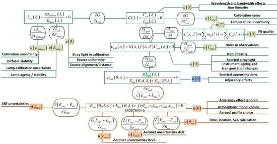
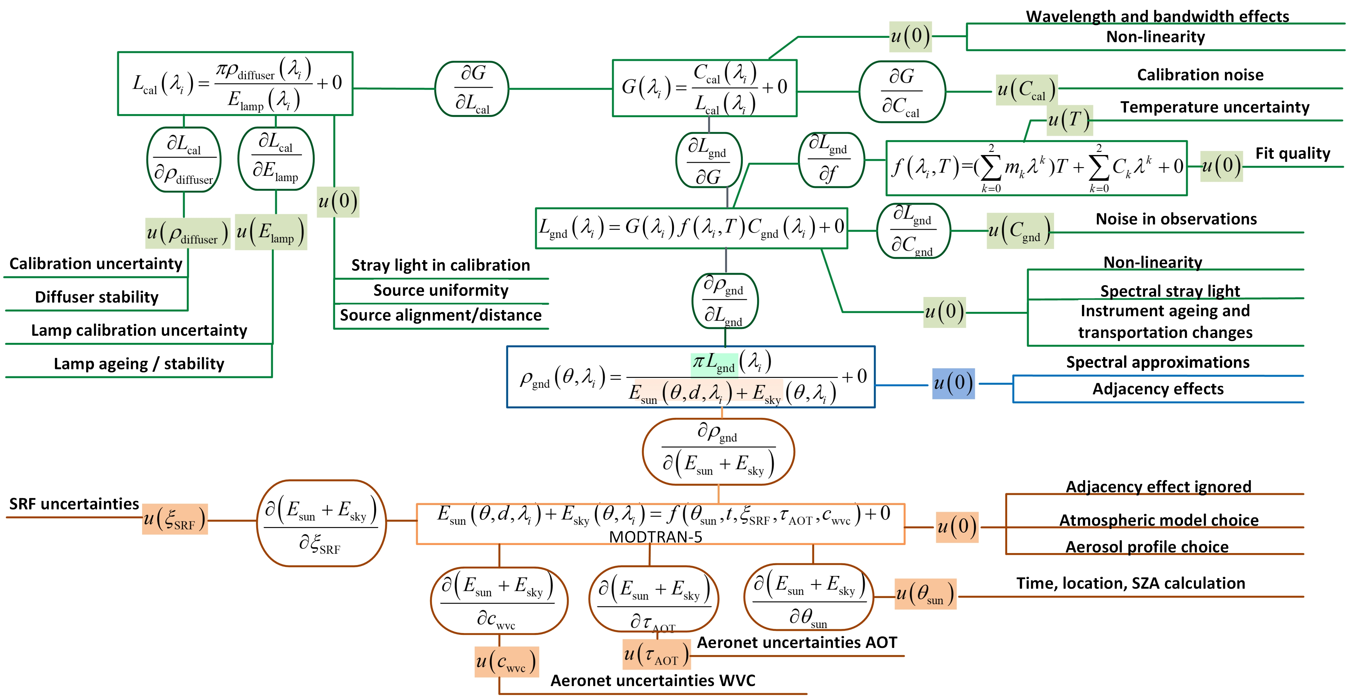
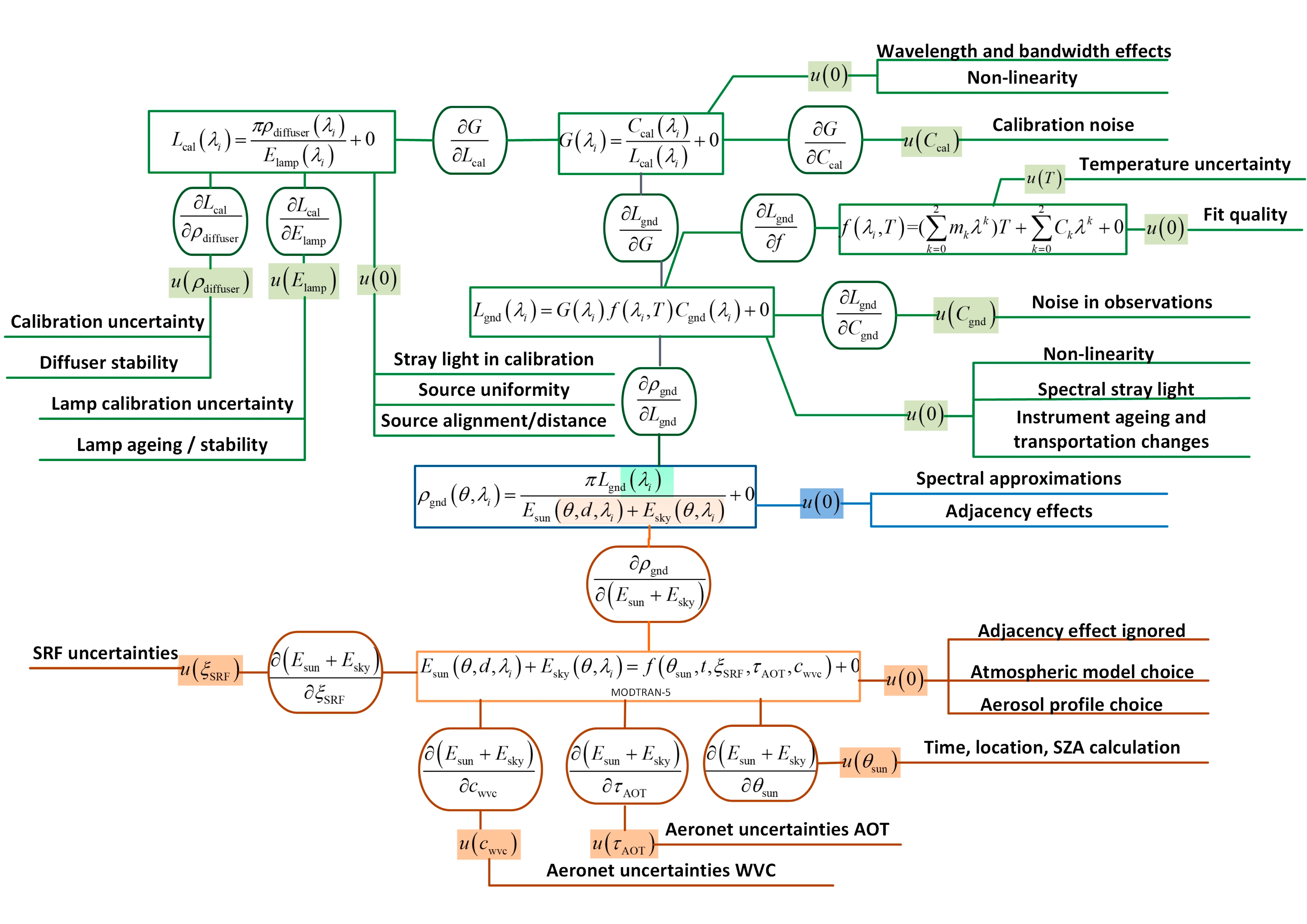
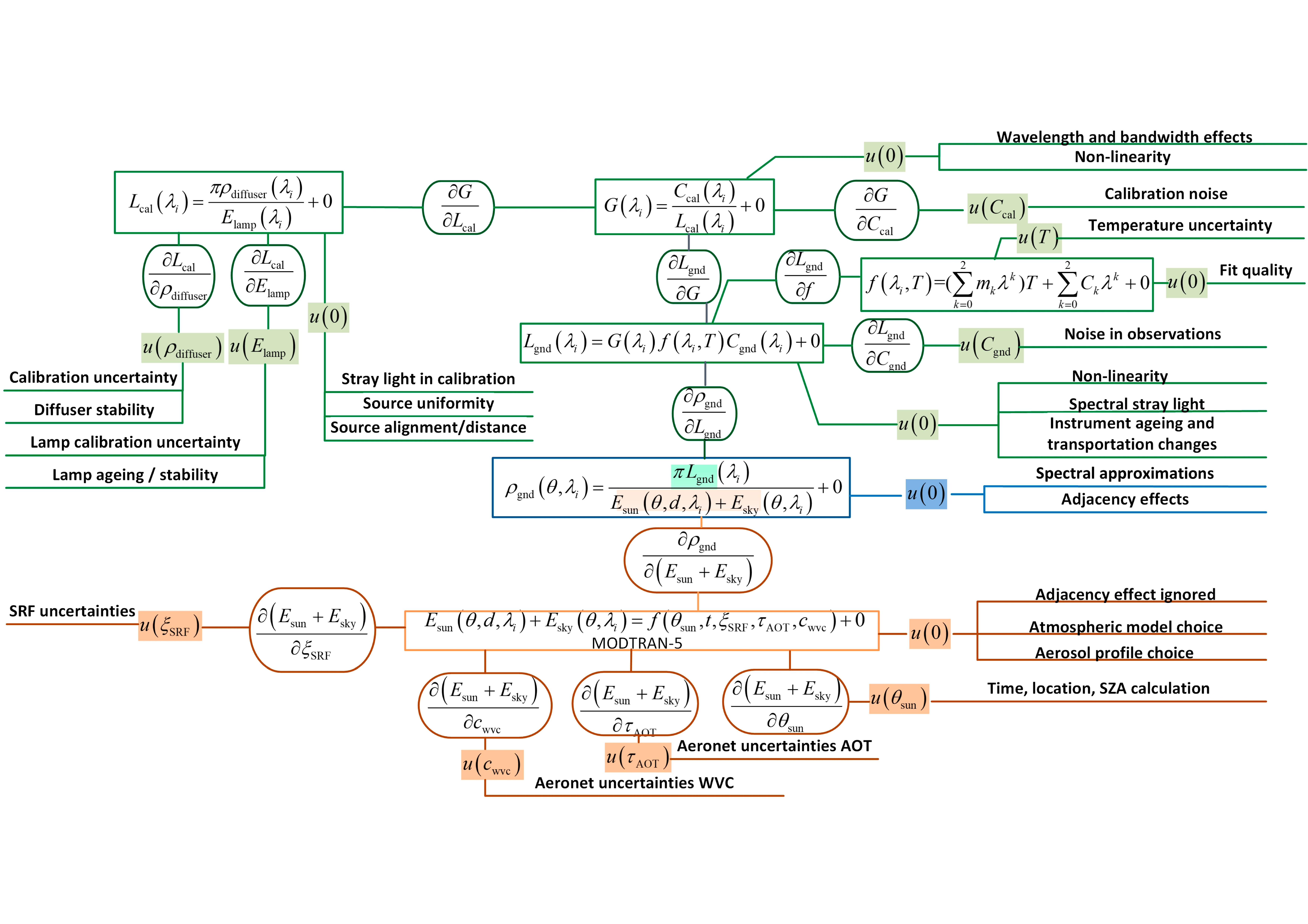
3.2.3. Uncertainty Tree Diagram

The uncertainty tree diagram is a conceptual diagram introduced in [11] which shows the origin of each term in the primary measurement equation (here Equation (1)). The diagram shows the sources of uncertainty that affect each term and gives the sensitivity coefficients—that is, the conversion factors that convert an uncertainty associated with an input quantity into the uncertainty associated with the measurand. Where an input quantity is itself calculated from its own input quantities, this is shown through additional sensitivity coefficients and equations. The sensitivity coefficients in any “branch” of the uncertainty tree can be multiplied together (chain rule) to provide the sensitivity of the primary measurand to the input quantity twig. Each source of uncertainty identified as a twig on this diagram should be evaluated both for magnitude and to understand the error correlation forms.
The uncertainty tree diagram for the Baotou measurements of ground spectral reflectance is given in Figure 4, which is reproduced at larger scale in Figure A1 (see Appendix A).

4. Results: Uncertainty Budget

4.1. Uncertainty Associated with Laboratory Calibration of the Field Spectrometer: Spectral Calibration

The spectrometers used at BTCN and BSCN were calibrated for wavelength accuracy and bandwidth using a mercury line source. The spectral radiance of the Hg source was determined, and from this for “clean” lines, with sufficient separation from other lines, a Gaussian distribution was fitted to the observed radiance. This provided an estimate of peak wavelength, which was compared to the Hg line wavelengths in air, and an (approximate) estimate of the instrument bandwidth. Note that future work is planned to characterize the spectrometer’s performance using a tunable laser system (see also Appendix B). This will provide improved information about the bandwidth and wavelength accuracy, which are limited here to the very small number of available cleanly separated spectral lines from the Hg source.
Across the spectrometer, the bandwidth (the standard deviation of the Gaussian fitted to the measured values) was consistently between 2.5 and 3 nm. This is wider than the MODTRAN-5 bandwidth assumption used in the solar and sky irradiance calculations. MODTRAN-5 uses a triangular bandpass function with a half base width of 10 cm−1, corresponding to 0.2 nm at 400 nm and 1 nm at 1000 nm. Note that the official RadCalNet product integrates over a 10 nm bandwidth.
The wavelength error of the spectrometer was approximately 1.7 nm (the spectrometer measured a wavelength that was 1.7 nm shorter than the true wavelength). No correction has been made until now for this wavelength error. To account for the uncertainty associated with the measured reflectance due to wavelength error, we need to consider both the impact on the calibration of the spectrometer gain using the calibration source and the impact on the field measurement. In both cases, the error can be approximated by:
δ ( L meas ) | δ λ   = L meas λ δ λ
where the first derivative can be estimated numerically. Using a balanced numerical derivative:
L meas λ 1 2 δ λ ( L k + 1 L k 1 )
we could estimate the error on each measured spectrum. We then calculated the ratio of the field measurement to the laboratory measurement with and without correcting this error. The results are shown in Figure 5.
To account for the time when this was not corrected, an uncertainty was applied to the measured signal that is 1.5% from 500 to 700 nm and from 780 to 900 nm, and ranges from 2% to 5% elsewhere. This is used rather than an error correction because the exact shape of the curve in Figure 5 will depend on the specific spectrum measured for each observation.

4.2. Uncertainty Associated with Laboratory Calibration of the Field Spectrometer: Radiometric Calibration

The laboratory calibration of the field spectrometer is described by Equation (3). It is calibrated against a known-radiance source made from a lamp-illuminated diffuser panel. There are uncertainties associated with each term in the measurement equation, and additional uncertainties associated with assumptions implicit in the measurement equation. These assumptions include assumptions about source uniformity and instrument linearity.

4.2.1. Lamp-Diffuser Panel Radiance

The lamp was calibrated for spectral irradiance on NIM’s primary facility through a direct comparison with a blackbody source. The uncertainties associated with this calibration have been documented previously and validated through comparisons as part of the Mutual Recognition Arrangement of national metrology institutes [14]. As is common for national metrology institute calibrations, the calibration certificate for the lamp provides uncertainties at the 95% confidence level. The standard uncertainty is obtained by dividing the certificate uncertainty by the certificate-provided coverage factor, here k = 2 for each wavelength value in turn. The lamp calibration was performed in 50 nm spectral steps and was interpolated to intermediate wavelengths using a cubic spline; the uncertainty was similarly interpolated.
There are additional uncertainties associated with the lamp spectral irradiance at the time of the spectrometer calibration due to lamp ageing since calibration and lamp current setting. The uncertainty associated with these quantities was estimated to be between 0.17% and 0.32% for all wavelengths through the annual stability of standard lamp and current setting of the power supply.
The diffuser was calibrated for spectral radiance factor on NIM’s reflectance facility as an absolute calibration; again the 95% confidence level uncertainty provided for each wavelength was converted to a standard uncertainty. The spectral radiance factor is defined as the “ratio of the radiance due to reflection of the medium in the given direction to the radiance of a perfect reflecting diffuser identically irradiated” in the International Lighting Vocabulary [16]
There are additional uncertainties associated with the distance setting and angular alignment of the lamp-diffuser pair. The lamp was set at 500 mm from the diffuser, which was the calibration distance for the lamp irradiance. However, because the diffuser is a bulk diffuser, the exact distance is difficult to set, and a residual distance uncertainty of 0.5 mm is assumed (from the inverse square law, a 0.5 mm uncertainty in 500 mm corresponds to a 0.20% uncertainty in irradiance). Similarly, the diffuser was calibrated for radiance factor for a 0°/45° geometry, and a spectrally-flat uncertainty of 0.20% was included to account for angular differences from this condition.

4.2.2. Source Non-Uniformity for Spectrometer Calibration

A source produced by a lamp-diffuser combination shows significant non-uniformity. Centrally with the lamp’s filament, the diffuser is at its brightest and this drops away from that central position (towards the outside and corners of the diffuser). This bright area may not align with the defined optical axis. The radiance of the panel is calculated from the irradiance of the lamp—which has in turn been measured over a small area around the optical axis—and the reflectance of the panel. The spectrometer used at Baotou has a field of view of 3°, and was set at 250 mm from the panel giving an observational area with diameter 13 mm.
The non-uniformity of the lamp-illuminated diffuser panel was measured at NIM. A CS-2000 spectroradiometer was used to measure the non-uniformity of diffuser, and the full field of view (FOV) of the spectroradiometer is 0.2°. The spectroradiometer at the same distance was used to scan the spectral radiance of the diffuser at 1 mm intervals over its surface. The measurement distance between the spectrometer and the diffuser is 250 mm, so the diameter of the field of view on the diffuser is 0.9 mm. The non-uniformity was calculated as the difference between an average radiance over the 13 mm area observed by the Baotou spectrometer and the point observation for brightest radiance. This was 0.29%.

4.2.3. Combined Uncertainty Associated with Source Radiance

The uncertainty associated with the source radiance comes from a combination of all the factors described above. These uncertainty effects are independent of each other and therefore inter-term error correlation does not need to be considered. However, we do still need to consider other error correlations. A single spectrometer is calibrated once a year against the lamp-diffuser panel radiance source. All uncertainties associated with that calibration will create an unknown calibration error that will be common for all measurements by the spectrometer in the field until the next calibration.
Because the same lamp and diffuser panel were used to calibrate all three spectrometers in position at BTCN and BSCN, many uncertainty effects will also lead to a common error between those spectrometers. An error in the lamp irradiance or diffuser reflectance will be common to all measurements by all spectrometers. However, an error due to the alignment of the lamp-diffuser panel combination will be different for each spectrometer as the system was entirely realigned between spectrometers.
We also need to consider error correlation scales from wavelength to wavelength. Uncertainties associated with alignment, distance, and stray light (all geometrical) create errors that are fully correlated between wavelengths. Any error in the lamp current setting will also be fully correlated from wavelength to wavelength, although as shorter wavelengths have a larger sensitivity to current setting, the uncertainty will be larger at shorter wavelengths (see Section 3.3.3 in [11] for a similar example). The lamp and diffuser calibrations at NIM create partially correlated errors from one wavelength to the next as some aspects of the primary calibration (e.g., alignments, reference blackbody temperature) are fully correlated and others (e.g., noise during calibration) are not correlated. As NIM repeated the calibration multiple times and had taken care to reduce the uncertainty associated with random effects as far as possible, the error correlation for these are “mostly fully correlated”.
The uncertainties associated with reference source radiance are listed in Table 1, which acts as an “effects table” (to use the term introduced in [11]).

4.2.4. Spectrometer Noise during its Calibration

The uncertainty associated with this noise in the calibration signal was estimated from the relative standard deviation of 20 successive measurements of the stable calibration source. The uncertainty associated with spectrometer noise is very close to zero at most of wavelengths, which was estimated to be less than 0.1%.

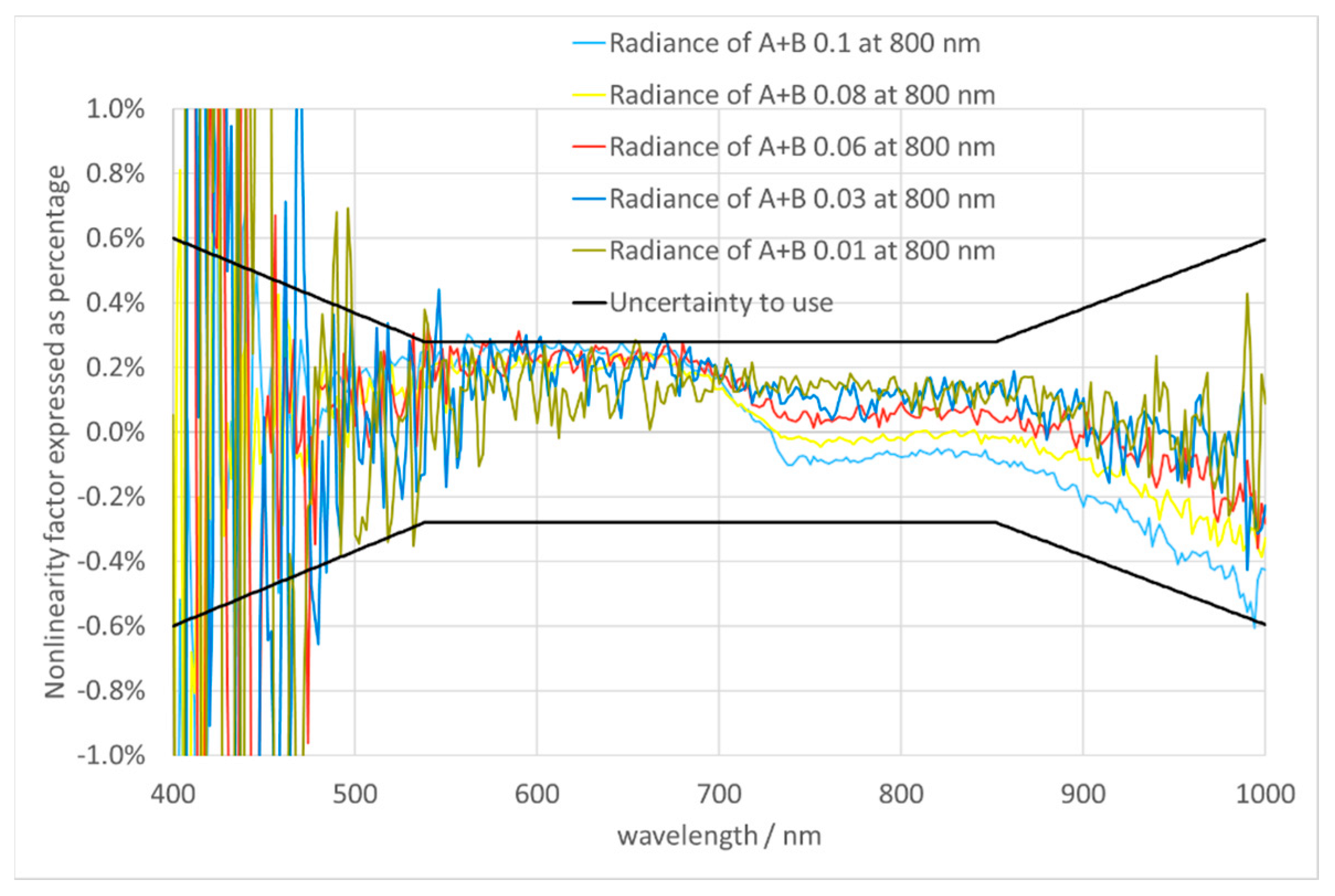
4.2.5. Spectrometer Nonlinearity

Equations (2) and (3) assume that the spectrometer is linear. We determine a single radiance calibration factor (radiometric gain) from a calibration against a single source at one radiance level. However, spectrometers often suffer from non-linearity [17], usually caused by processes in the read-out electronics. There are two types of nonlinearity that must be considered: radiance level nonlinearity (gain is not constant with changing radiance) and integration-time nonlinearity (the measured counts are not proportional to the integration time). To evaluate these nonlinearities, the spectrometer was tested using a special integrating sphere system designed by NIM. The spectrometer remained on its “auto ranging” setting, so the integrating time varied dynamically.
The integrating sphere is illuminated by two lamps, each with an adjustable aperture in front of it. In this way the overall radiance of the sphere could be varied and each lamp in turn could be closed off. The sphere’s spectral radiance was varied so that at 800 nm it ranged from 0.005 to 0.25 W m−2 sr−1. The normal calibration radiance at 800 nm is 0.071 W m−2 sr−1 and the grey target radiance at 800 nm ranges between 0.005 W m−2 sr−1 (lowest typical values) and 0.1 W m−2 sr−1 (highest typical values).
The nonlinearity factor σ of the spectrometer is calculated as:
σ = I ( A + B ) I ( A ) + I ( B ) 1
where I ( X ) is the response of the spectrometer for a radiance level X , where X is the source with only lamp A, with only lamp B, or with lamps A and B simultaneously. The results are shown in Figure 6 and show an increase in nonlinearity for the shortest and longest wavelengths. Because nonlinearity is not corrected in the measurements during calibration or in the field, we treat the observed non-linearity as an uncertainty component. At the shortest wavelengths it is difficult to separate nonlinearity from noise, but taking into account that nonlinearity is unlikely to be significantly different from pixel to pixel, an uncertainty curve has been approximated using a local standard deviation. At longer wavelengths there is a noticeable trend, and uncertainty bounds have been drawn to include this trend. From this we assume that the uncertainty associated with nonlinearity is 0.28% from 540 nm to 850 nm, increasing to 0.6% linearly for longer and shorter wavelengths.

4.2.6. Stray Light during Calibration and Field Operation

Equation (3) assumes that the measured count signal comes from the source radiance, both in the laboratory and in the field environment. In practice there are several effects that alter this assumption.
First, there may be an electronic bias, a “dark count”, that is present when there is no illumination. This dark count is likely to be temperature sensitive and thus will change over time. In the laboratory the dark count can be measured by closing the input optics. In the field, such measurements are not possible routinely, but some tests can be performed manually. Beyond 500 nm the ratio of dark signal to light signal is less than 0.1%.
Second, there may be external stray light that reaches the instrument sensors from outside the main field of view. In the laboratory such stray light will come from any reflections of the source into the beam. In the field, it will come from the bright surrounding area. This is discussed in Appendix B.1. The uncertainty associated with this stray light has been estimated to be 0.1% for all wavelengths.
Third, there is internal stray light. Internal stray light comes from light that is scattered onto the “wrong” pixel from the wrong wavelength. Appendix B discusses how the stray light was evaluated using cut on filters. The error associated with not correcting for stray light is 25% at 400 nm, dropping to 10% at 420 nm, 5% at 440 nm, and 3% at 460 nm. While Appendix B provides a method that could be used to correct for stray light, in practice this has not been applied to data collected at BTCN and BSCN to date. The RadCalNet WG has agreed to operate with a “collection” process, where data that are on the portal can only be updated retrospectively at defined times, known as “collections” and the next collection is likely to be during 2021. Therefore, at present there is no stray light correction and a correction cannot be performed until 2021. Thus, the uncertainty is at its full magnitude. By the next collection we hope to have calibrated the instruments using tunable lasers so that the full correction algorithm discussed in Appendix B.3 can be applied.

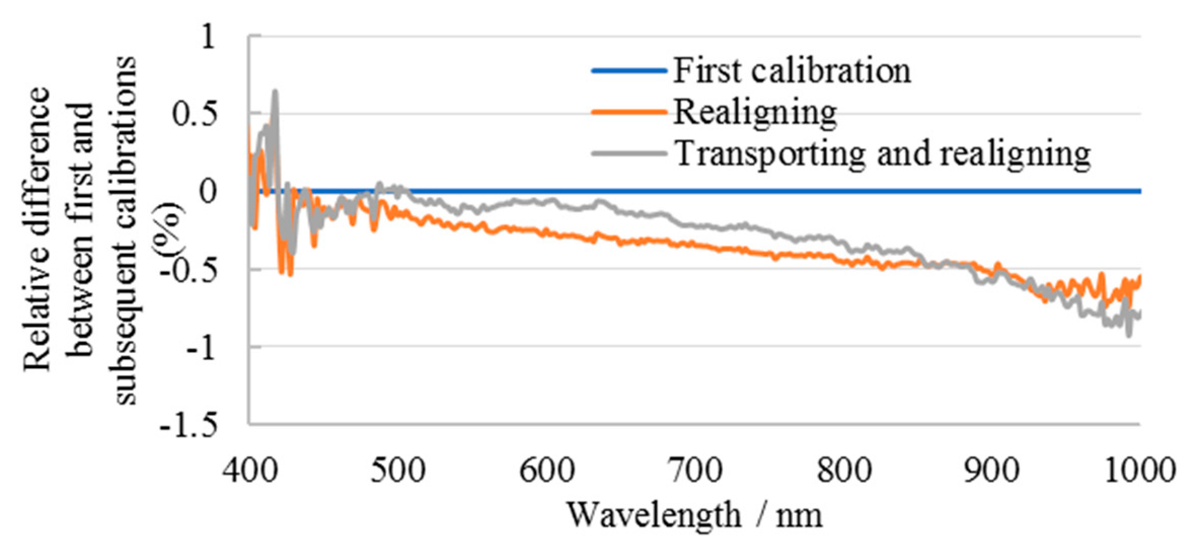
4.2.7. Repeatability of the Calibration/Transportation Stability

The repeatability of the calibration and the sensitivity of the spectrometer to transportation was tested using a stable laboratory source at NIM. The spectrometer was calibrated on three occasions: twice while realigning but not transporting the instrument, and a third occasion where the instrument was transported then realigned. The relative difference of the second and third calibrations compared to the first calibration is shown in Figure 7. This suggests that the dominant effect is realignment. For the purposes of this analysis the uncertainty associated with transportation is less than 0.5%.

4.2.8. Combined Uncertainty Associated with the Laboratory Calibration of the Spectrometer

The combined uncertainty associated with the laboratory calibration of the spectrometer is a combination of the effects given in this section. Table 2 lists the different effects, the magnitude of their uncertainty, and the error correlation structures. The uncertainty associated with source radiance is obtained by combining the different components in Table 1. The wavelength accuracy is a setting of a spectrometer. In this way the associated error is fully correlated for all observations with that spectrometer and it is independent between spectrometers. Because the wavelength error changes across the spectrum, we consider its error partially correlated from wavelength to wavelength, however, the error is dominated by a common component. Noise is naturally entirely independent from observation to observation and because external stray light is a property of the calibration set up, this is considered to have a fully correlated error. Nonlinearity and internal stray light are properties of the spectrometer and have a stable spectral feature. Finally, calibration repeatability, which includes the stability of the instrument on transfer to the field, has an error considered to be fully correlated for all measurements by that spectrometer but independent between spectrometers.

4.3. Uncertainty Associated with the Field Measurement of Radiance

In this section we consider uncertainties associated with the measured field radiance obtained from Equation (4). Uncertainties associated with the calibration of the instrument, described above, affect the gain term, noise affects the measured in-field signal, and the temperature correction has uncertainties related to the uncertainty in the instrument in-field temperature, and the uncertainty associated with our knowledge of the coefficients and form of the correction Equation (5). Uncertainties associated with the stability of the instrument gain have already been considered in the “calibration repeatability” term in the section above and are not included here to avoid double-counting.

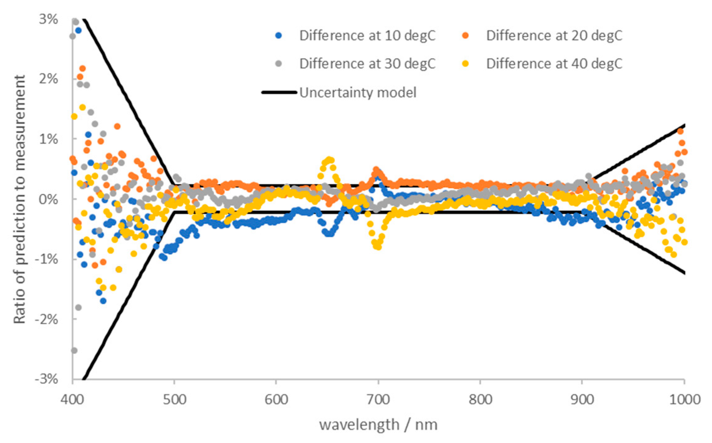
4.3.1. Spectrometer Temperature Stability

Equation (5) gives an empirically determined model for the temperature correction. This was obtained by calibrating the instrument against a stable source while its temperature was varied from 10 to 40 °C and the results compared to the reference calibration at 25 °C. The fitted curves as a function of wavelength are shown in Figure 8.
To work out the uncertainty associated with this correction, there are two components. First the uncertainty associated with the gain correction due to an uncertainty in instrument temperature of 2 °C can be estimated by applying the law of propagation of uncertainty to Equation (10). Here the notation u ( G T ) | u ( T ) describes the uncertainty associated with the gain at a temperature T due to the uncertainty associated with that temperature u ( T ) . This is used because there are other uncertainties associated with the gain that would need also to be considered in a full uncertainty analysis of the gain.
u ( G T ) | u ( T ) G cal ( λ ) = 1 G cal ( λ ) G T T u ( T ) = ( m 0 + m 1 λ + m 2 λ 2 ) G cal ( λ ) u ( T ) .
Second, there is an uncertainty associated with the plus-zero term in Equation (5). This is the uncertainty associated with the suitability of the model to represent the true temperature sensitivity of the instrument. This uncertainty was estimated from the residual of the original measurement points to the model (Figure 9). The uncertainty associated with temperature correction includes both the propagated uncertainty (due to a 2 °C uncertainty associated with the temperature of the instrument in the field) and the model uncertainty given here.

4.3.2. Noise in the Field Measurements

During field measurements a single reading is taken every two minutes with an integration time determined automatically. The uncertainty associated with noise on this measurement cannot therefore be estimated from operational data.
However, to complement the laboratory measurements of repeatability described above in Section 4.2.3, 20 measurements were taken in the field within 30 s. The standard deviation of those 20 measurements was slightly higher than the 0.1% seen in the laboratory and ranged from 0.4% at 400 nm to 0.1% at 600 nm.

4.3.3. Combined Uncertainty Associated with the Field Measurement of Radiance

The combined uncertainty associated with field radiance measured by the spectrometer is obtained by combining the different components in Table 3. We have not performed that combination at this stage because we want to combine uncertainties with different error correlation structures separately. The measurement noise during a single field measurement leads to an error that is entirely independent from one measurement to the next, from one spectrometer to the next, and from one wavelength to the next. For the uncertainty associated with the temperature sensitivity coefficient, this can be considered fully correlated for all measurements by a single spectrometer (the effect is stable) and independent between spectrometers, because there is a separate thermometer in each spectrometer and they are mounted in separate housings, and because the effect was separately calibrated for each spectrometer. The wavelength-to-wavelength error correlation structure is mixed. Figure 9 above shows that the residual has almost no spectral pattern (except perhaps for central wavelengths where it is small) and therefore it is reasonable to assume that the error is uncorrelated. On the other hand, the propagation from an uncertainty associated with temperature to that associated with scene radiance is fully correlated between wavelengths as is related through an algebraic expression.

4.4. Uncertainty Associated with the Ground Reflectance

4.4.1. Atmospheric Measurements from the AERONET Sun Photometer

The ground-measured radiance is converted into ground reflectance using Equation (1). This equation requires an estimate of the solar irradiance as transmitted through the atmosphere and the sky irradiance as scattered by the atmosphere. Both quantities are evaluated using MODTRAN-5, which requires atmospheric parameters as inputs.
These atmospheric parameters are measured using the Cimel CE318 sun photometer which is at the Baotou site. The sun photometer forms part of AERONET and has been calibrated according to the AERONET procedures [9], originally at NASA and more recently at the Beijing XMWK Technology Co. Ltd., China. The measurement data are transmitted to the AERONET data processing center, automatically processed and made available at the AERONET website. Then, the aerosol optical depth (AOD) at 550 nm is calculated via logarithmic interpolation from the AOT in the 440, 670, 870, and 1020 nm channels. The measurements in the 936 nm channel of the solar radiometer are used to calculate the water vapor column (WVC), using a modified version of the Langley algorithm [18]. We have taken the uncertainties associated with AOD and WVC from the literature, in particular [19]. These are estimated as less than 0.01 (absolute uncertainty) and less than 12% (relative uncertainty), respectively.

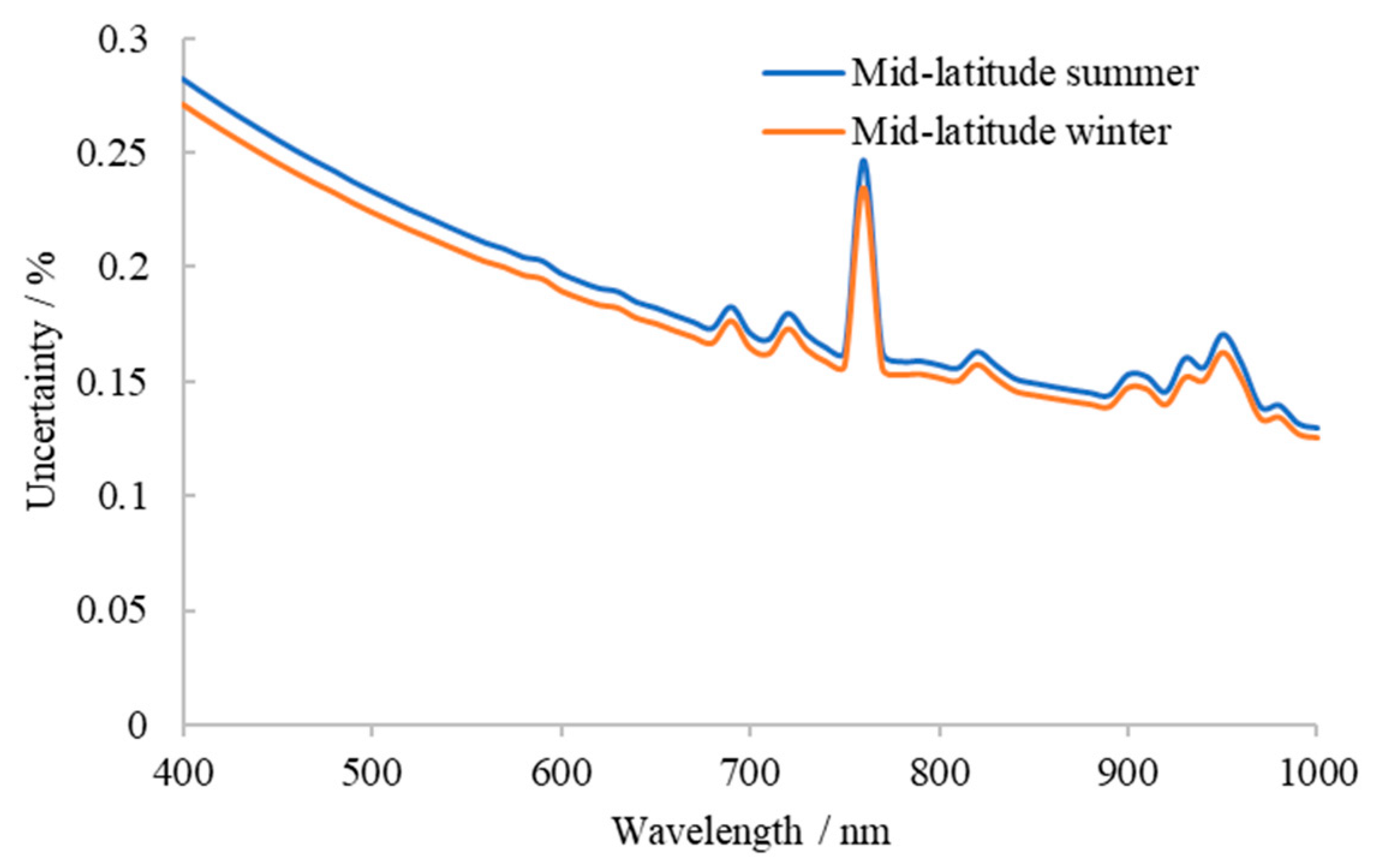
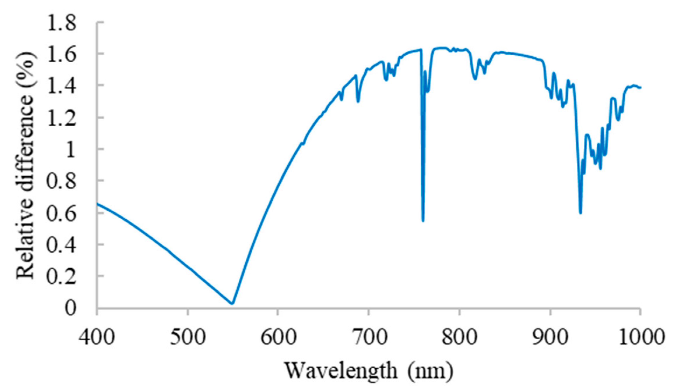
4.4.2. Sensitivity Analysis of MODTRAN-5 to Atmospheric Conditions

Monte Carlo (MC) analysis techniques were used to determine the sensitivity of the MODTRAN-5 sky irradiance and solar irradiance calculations to uncertainties in the input parameters. Errors drawn from a Gaussian distribution with a standard deviation of 12% (relative) and 0.01 (absolute) were added randomly to WVC and AOD respectively, for a range of realistic conditions for the Baotou site. Each combination of parameters was separately tested, with for each test, either the AOD or the WVC varied and the other component kept constant. The corresponding total downwelling irradiance, i.e., the relative uncertainty associated with E sun ( θ , d ; λ i ) + E sky ( λ i , t ) in Equation (1), was simulated 1000 times by MODTRAN-5. The standard deviation of each 1000 sets of simulated irradiances was the uncertainty associated with downwelling irradiance due to AOD or WVC uncertainties. A further test was performed where these two parameters were varied together (in a way that was consistent with the fact they were derived together, so including any error correlations) and this gave the same uncertainty as the combined uncertainty from the two separate components.
Figure 10 shows the relative uncertainty associated with the total downwelling irradiance due to WVC uncertainties of 12%. Similarly, Figure 11 shows the relative uncertainty associated with the total downwelling irradiance due to AOD uncertainties of 0.01. These graphs are for two of the representative conditions studied; similar results were obtained for other conditions. In the MC simulations, the mean value of AOD is set as 0.2, the mean value of WVC is set as 0.5 g/cm2, and solar zenith angle (SZA) and view zenith angle (VZA) are set as 30° and 0°, respectively.

4.4.3. Other Uncertainties Associated with the MODTRAN-5 Processing

In addition to the uncertainties associated with the input parameters to MODTRAN-5 (the AOD and WVC), the downwelling irradiance calculated by MODTRAN-5 has uncertainties associated with other assumptions in the MODTRAN-5 model. MODTRAN-5 makes assumptions on the heights of different atmospheric layers and defines a set of “atmospheric models” to describe these conditions. It also makes assumptions on the type and size of aerosols and defines a set of defined “aerosol models” to describe different assumptions. For Baotou two atmospheric models are used, i.e., the one defined as “mid-latitude summer” is used from April to September and the “mid-latitude winter” model is used from October to March.
The aerosol model used is the “rural” type. This was chosen because the site is 70 km from the nearest city, Baotou, China. It is possible that the “desert” aerosol type may be more appropriate for some periods of the year. To understand the difference between “desert” and “rural” aerosol models for the site, data from one measurement were processed using both aerosol models. The relative difference between the models is given in Figure 12. The uncertainty associated with aerosol type is taken to be a rectangular distribution within this range, thus the standard uncertainty is D / 2 3 , where D is the full difference (Figure 12).
The overall accuracy of the MODTRAN-5 evaluation of downwelling irradiance also depends on the uncertainty associated with the radiative transfer model within MODTRAN-5 and the uncertainty associated with the solar spectral irradiance model used. Uncertainties associated with the solar zenith angle and solar distance (θ, d, respectively, in Equation (6)) are considered negligible. In the future, this uncertainty estimate could be evaluated using in-field measurements, but that has not yet been done.
The uncertainty associated with the MODTRAN-5 radiative transfer model is described in the literature [20] as being 1%–2% for radiance predictions. The solar spectral irradiance model used is the Thuillier model [15,21] and this has a standard uncertainty of 1.5% at 450 nm, 0.9% at 650 nm, 1.1% at 850 nm, and 0.8% at 1550 nm. As the spectral uncertainty is not known, these values at 450, 650, 850, and 1550 nm were linearly interpolated to provide intermediate wavelength uncertainties.

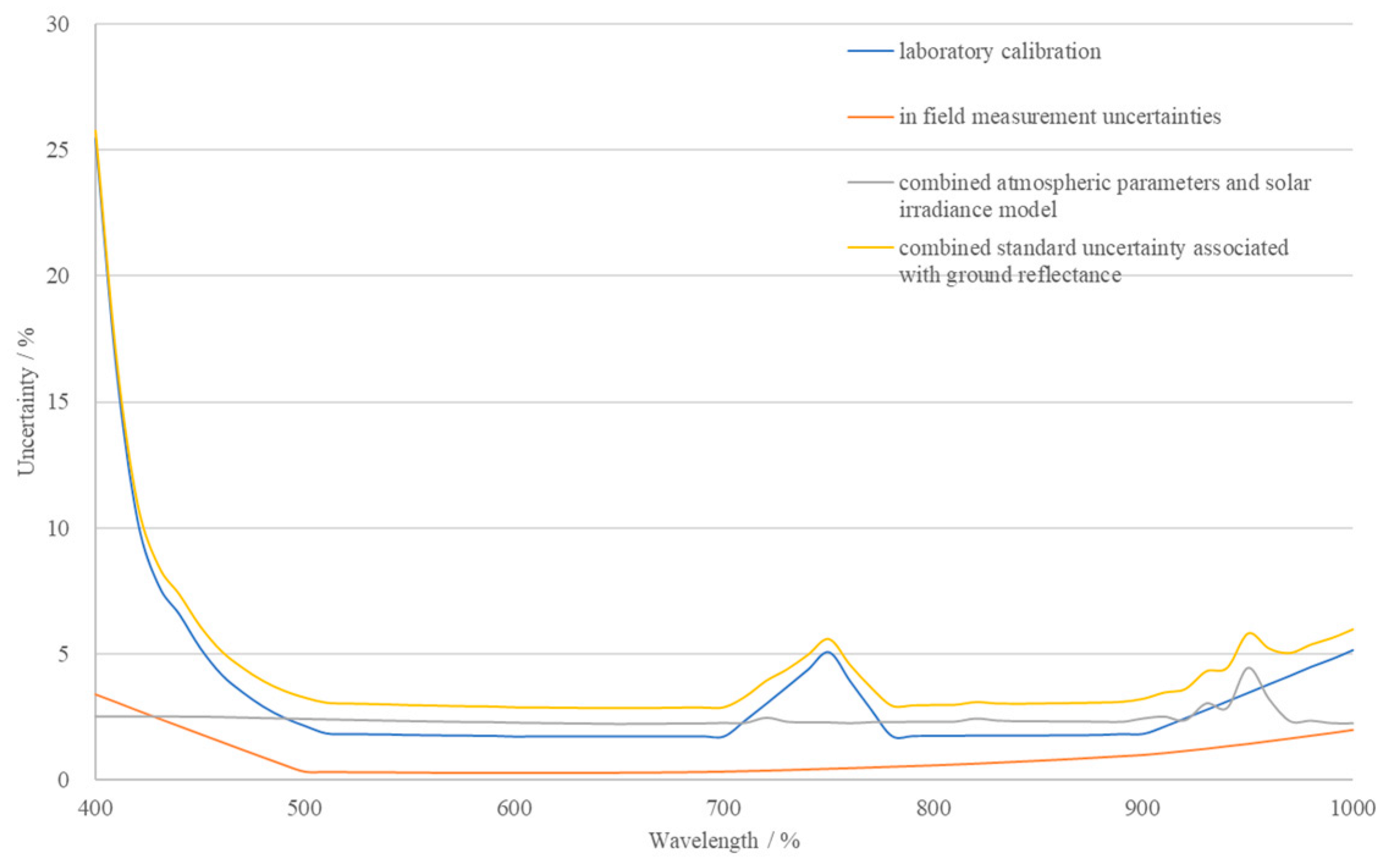
4.4.4. Combined Uncertainty Associated with Ground Spectral Reflectance

Overall, ground reflectance is calculated using Equation (1). As we have considered in the previous subsections the total downwelling irradiance E sun ( θ , d ; λ i ) + E sky ( λ i , t ) as a single quantity, we also do not separate them in our combined uncertainty table. The combined uncertainty associated with ground reflectance are obtained by combining the different components in Table 4. Figure 13 shows the uncertainty associated with the bottom-of-atmosphere (BOA) reflectance from 400 nm to 1000 nm.
The error correlation structures due to the solar and sky irradiances are considered partially correlated from one observation to the next with a single spectrometer; the assumption is that these change on longer time scales (hours to days), but are constant for shorter timescales. This assumption could be refined by assuming a triangular or bell-shaped correlation structure but that has not yet been analyzed. Between spectrometers the error correlation is considered fully correlated—the three spectrometers are all on the same super-site and the same AERONET CIMEL instrument is used to obtain corrections for all three instruments. To evaluate the error correlation structure between wavelengths, we analyzed the Pearson correlation coefficient for the errors obtained in the Monte Carlo simulation. This showed a very high error correlation (above 0.95) for almost all wavelengths. We therefore treat this as fully correlated from wavelength to wavelength. The same analysis has not been done for the solar irradiance model, but we assume that it is also fully correlated for the purposes of a precautionary analysis (fully correlated components are not reduced by averaging).

4.5. Uncertainty Associated with the RadCalNet BOA Reflectance Product

The BOA reflectance measurement uncertainty established in the previous section is for a measurement with a single spectrometer at a single time at the native wavelengths of the spectrometer. These measurements are every 2 min on site. For the official RadCalNet BOA reflectance product we (a) increase the wavelength step to 10 nm, (b) provide a product for the full site area (45 × 45 m for BTCN, 300 × 300 m2 for BSCN), and (c) average readings to create a value every 30 min.

4.5.1. Wavelength Sampling

To obtain data at 10 nm intervals there are two options. One option is to provide the narrow bandwidth information at 10 nm intervals. The other option is to perform a spectral integral to combine data over a 10 nm bandwidth. At present, the Baotou 10 nm data are obtained by picking the data at the 10 nm intervals. Therefore, this does not alter the uncertainty analysis.

4.5.2. Representativeness (Site Homogeneity)

The measurement of the site reflectance by the spectrometers is at one point (for BTCN) or two points (BSCN). However, the satellite observations will be averaged over the larger area of the defined site. To understand the representativeness of a single/two measurement(s) for the site as a whole, tests were performed where a portable spectrometer was used to make measurements at multiple points across each target. The spectrometers have a field of view of 3° and therefore see an area with a diameter of ~104 mm for BTCN (2 m above ground), and ~131 mm for BSCN (2.5 m height). For BSCN, the site is a natural sand with a ~1 mm grain size. For BTCN, the site has pebbles which are typically ~15 mm across. The portable spectrometer used for this analysis imaged a similar area to the permanent instruments.
The uncertainty associated with the representativeness of the point measurement was estimated based on the uniformity of the whole target, which is defined using the following equation:
u ( λ ) = 100 % × σ ( λ ) ρ ¯ ( λ )

4.5.3. 30 Minute Temporal Averages

To obtain BOA reflectance every 30 min, the reflectance averages of 15 min before and after a given time (i.e., 9:00, 9:30, 10:00, etc.) are used as the final BOA reflectance. Since the measurement interval of spectrometer is 2 min, 15 BOA reflectance values are averaged. The variation in those readings comes from two origins: first, we expect variability due to all the effects listed in the tables above that have “independent” as their reading-to-reading error correlation structure and second, we expect variability due to the change in solar zenith angle over the 30 min averaging period. To validate the uncertainty associated above with “independent” effects we compared the standard deviation of the 15 readings with the combined uncertainty and obtained close agreement at noon. At 9 am and 3pm, the standard deviation was higher than the combined uncertainty of the “independent” effects, because of the change in the solar zenith angle. However, at present no uncertainty has been introduced to account for solar zenith angle changes as the time period of averaging is symmetrical about the declared time and the difference between the measured mean and a mean corrected for solar zenith angle is negligible.

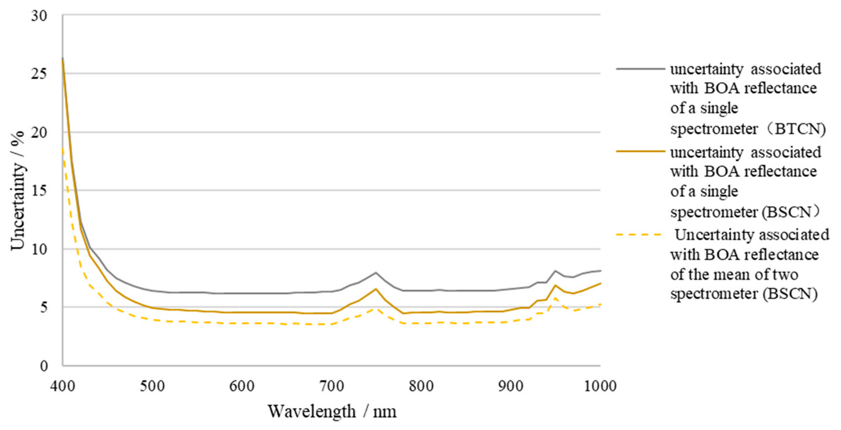
4.5.4. Uncertainty Associated with the BOA Reflectance

The combined uncertainty associated with the BOA reflectance is a combination of the effects given in Section 4.1, Section 4.2, Section 4.3, Section 4.4 and Section 4.5. For BTCN and BSCN for the initial period when only one spectrometer was in operation, the official RadCalNet product is the uncertainty associated with the temporal mean of 15 measurements with a single spectrometer. To establish the uncertainty associated with this mean, we combined uncertainties that were associated with errors that were “partially” or “fully” correlated with time (any partial correlation is likely to be extremely high over a 30 min window) and separately combined uncertainties associated with errors that were “independent” in their error correlation structure. The uncertainty associated with independent effects could be reduced by the square root of the number of independent observations, here 15 , and this was then added in quadrature (square root of the sum of the squares) with the uncertainties associated with correlated effects.
For the calculation of the uncertainty associated with the mean of the two spectrometers at BSCN, the uncertainty components were separated into (a) fully correlated for both time and between spectrometers, (b) fully independent for both time and between spectrometers, (c) correlated between spectrometers but independent from measurement to measurement, and (d) correlated between measurements but independent between spectrometers. Then, we separately calculated the uncertainty associated with each of these. The uncertainty associated with the mean of two spectrometers based on 15 measurements each was calculated by dividing (a) by 1, (b) by 30 , (c) by 15 , and (d) by 2 . Finally, the combined uncertainty was calculated as the square root of the sum of the squares of these four parts. For this combination, we have assumed that the atmospheric effects are fully correlated over the 30 min of the averaging.
Figure 14 shows the uncertainty associated with the BOA reflectance. A summary for the uncertainty budget of BTCN and BSCN BOA reflectance is shown in Table A1 (see Appendix C).

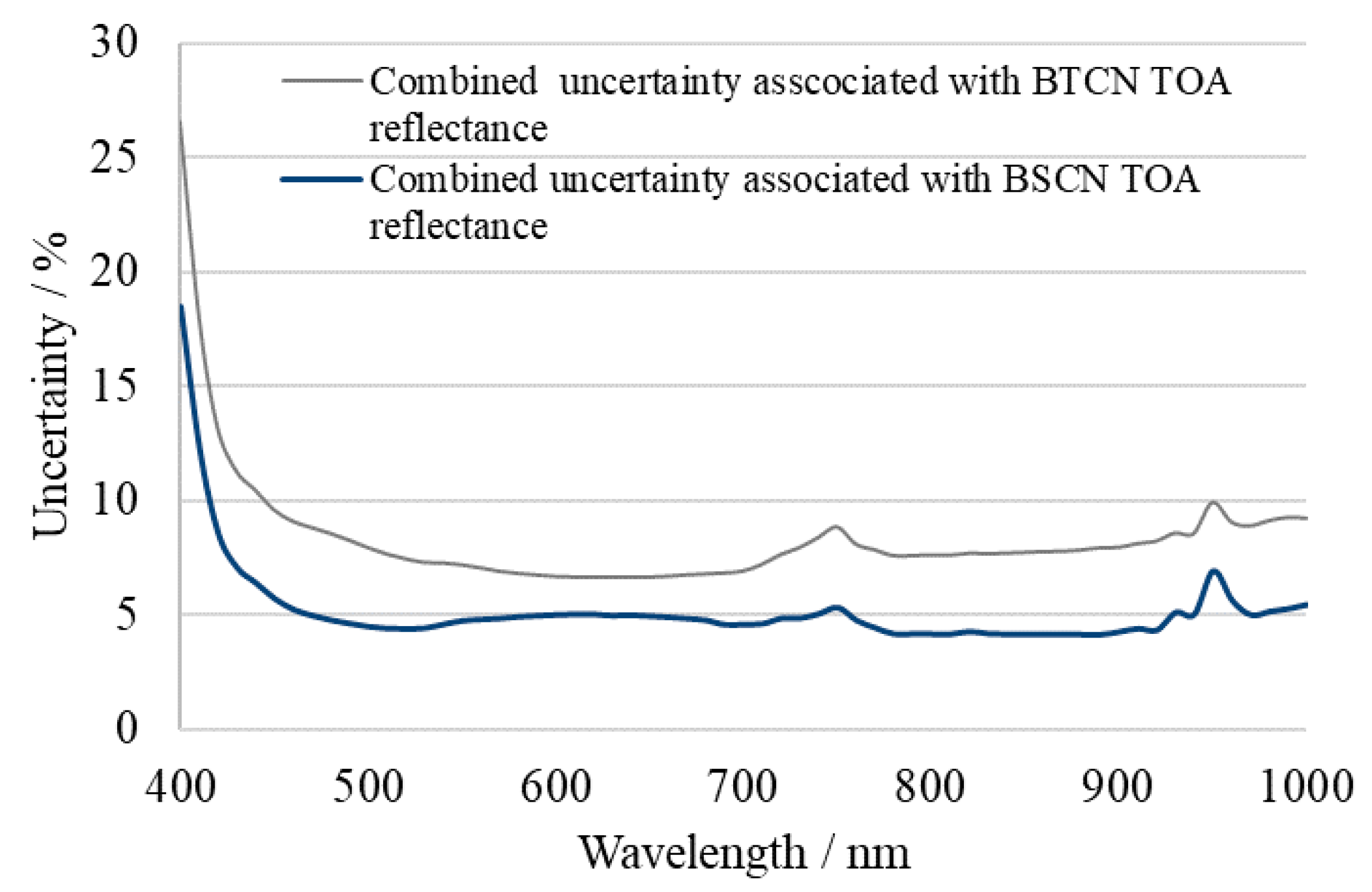
4.6. Uncertainty Associated with Propagation to TOA

Comparing a satellite sensor observation with the Baotou calibration site requires TOA reflectance. As discussed in Section 3.1, propagation to TOA requires the determination of direct light from the site, light lost through scattering between the site and the satellite, and light gained from scattering in the atmosphere, both directly and having reflected off nearby ground locations. The influence on the measured radiance of light that has reflected off nearby ground locations (background radiation) is described by the adjacency effect [22].
AIR has performed a detailed analysis on the adjacency effect when calculating the TOA reflectance from the BOA reflectance. A method considering the adjacency effect has been proposed and detailed in another paper [23]. In this method, a local atmospheric point spread function (PSF) for the Baotou site was constructed, and this was used to calculate an effective background reflectance that was used in MODTRAN-5 simulation as the reflectance of the surrounding area. The TOA reflectance calculated using this method with the consideration of adjacency effect was compared with several satellites’ observations. The uncertainty associated with the effective background reflectance was obtained by considering several uncertainty components, such as the constructed atmospheric PSF, the error of AOD, and the seasonal change of the surrounding area. Then, the uncertainty associated with the TOA reflectance simulated using the effective background reflectance was also estimated.
However, for the official RadCalNet product, the propagation to TOA is performed through the RadCalNet processing. This does not have the option to include the correction of the adjacency effect. Thus, we determined the uncertainty introduced by not correcting for the adjacency effect, based on the constructed effective background reflectance of Baotou site in the previous study. This was evaluated by running MODTRAN-5 for the different targets assuming first the background reflectance discussed above and then a background reflectance that is the same as the target reflectance. The difference in the TOA reflectance between correcting and not correcting the adjacency effect in MODTRAN-5 simulations for BTCN and BSCN targets are shown in Figure 15.
In addition to the uncertainties associated with the BOA reflectance measurements, uncertainties associated with the radiative transfer modelling to TOA performed by MODTRAN using the input atmospheric conditions, such as AOD, WVC, aerosol type, and MODTRAN model, are also considered. To determine the uncertainty associated with propagation to TOA reflectance, a similar approach to that used for the determination of the uncertainty associated with E sun ( θ , d ; λ i ) + E sky ( λ i , t ) was used (Section 4.4). The TOA reflectance is calculated using MODTRAN-5 from solar spectral irradiance, sun–earth distance factor and the solar zenith angle. MC analysis techniques were also used to determine the uncertainty associated with the TOA radiance due to WVC and AOD uncertainties. The uncertainties associated with the assumption of aerosol type, solar irradiance model, and MODTRAN-5 radiative transfer model were also considered.
According to the analysis results, the total uncertainty associated with the TOA reflectance propagated from the BOA reflectance is given in Figure 16.

5. Discussion

The uncertainty of BOA reflectance (strictly “hemispherical-conical reflectance factor”) measured by a single spectrometer for BTCN (about 6%) is greater than that for BSCN (about 4.8%), which is to a large extent caused by the surface uniformity. Because there are two spectrometers deployed in BSCN, the uncertainty for BSCN is further decreased to about 3% across most of the wavelength range (see Figure 14). Thus, the combined uncertainty of BSCN associated with propagation to top-of-atmosphere reflectance is almost always better than 5% within the spectral range 450–1000 nm, and in about half of the spectral range the uncertainty is less than 4%. This result indicates that the high uncertainty due to the poor surface uniformity for the BTCN site could be reduced by using multiple observation devices. At the shortest wavelengths (below 450 nm) the uncertainty is dominated by internal stray light effects within the spectrometer and reaches ~20% at 400 nm.
This paper focuses on the uncertainty analysis method applied to the official RadCalNet reflectance products using the standard RadCalNet processing, without adjacency effect correction and at 10 nm intervals. Reduced uncertainties are available from a processing to TOA that includes adjacency effect correction.
Performing a thorough uncertainty analysis always identifies areas of potential improvement. Here we have identified that the wavelength error could be reduced and that stray light is the dominant source of uncertainty for the shortest wavelengths and therefore needs a more thorough investigation and the establishment of a matrix-based correction algorithm. We anticipate that these investigations will lead to an improved uncertainty by the time of the next RadCalNet Collection (2021) and some of the corrections will be able to be applied retrospectively (particularly for stray light). The uncertainty associated with homogeneity is also a significant uncertainty for BTCN and could, perhaps, be improved using an instrument with a wider field of view, however, such an instrument would be more difficult to calibrate. The uncertainty budget allows us to consider such trade-offs in future improvements.

6. Conclusions

This paper showed an example of a metrological uncertainty analysis for a RadCalNet site. For the first time, we considered the error correlation structures for each uncertainty component. These error correlation structures enabled us to perform a robust propagation to a product that averages two spectrometers and 15 measurements by each spectrometer. In the future, we will use the wavelength-to-wavelength error correlation structure to obtain a reliable estimate of the uncertainty associated with a spectrally integrated product (e.g., to match the spectral response function of a satellite sensor). The temporal and spectrometer-to-spectrometer error correlation structures will also be needed to determine a robust uncertainty associated with the comparison to a satellite that makes multiple overpasses of the sites during a comparison period. To perform that analysis completely, we would also need to account for the error correlation structures for the satellite product. The paper that we used as the basis of the method described here [11] has shown how this was done for the Advanced Very High Resolution Radiometer (AVHRR) sensors. A simplified version of this has also been done for Sentinel-2 [24].
As an example of the metrological uncertainty analysis, this paper described the determination of ground reflectance and TOA reflectance for the Baotou BTCN and BSCN sites. We analyzed the sources of uncertainty from the laboratory calibration of the spectrometer, through to field observations of radiance and the calculation of ground reflectance, and to the propagation to TOA reflectance. The uncertainty tree diagram for the Baotou measurements of ground spectral reflectance was drawn, and every uncertainty component was considered and analyzed based on tests in the laboratory and field, and Monte Carlo modelling of the atmospheric corrections.
The preliminary results for the uncertainty propagating to the TOA reflectance were analyzed. The uncertainty associated with the TOA reflectance propagated from BOA reflectance measured by a single observation is approximately estimated as 6% for BTCN and 4.8% for BSCN if the adjacency effect can be corrected for. Since the RadCalNet BOA product on BSCN is generated based on the observations from two spectrometers, its uncertainty is reduced to about 3%. The uncertainties of the official RadCalNet TOA product (which does not consider the adjacency effect) for BTCN and BSCN are estimated to be approximately 7% and 4%–5%, respectively.

Author Contributions

Conceptualization, L.M. and E.R.W.; Formal analysis, Y.Z.; Methodology, L.M., Y.Z., E.R.W. and C.D.; Supervision, C.L. and L.T.; Validation, N.W., Y.L., L.L. and C.G.; Writing—original draft, L.M., Y.Z. and E.R.W.; Writing—review & editing, X.W., E.R.W., L.M. All authors have read and agreed to the published version of the manuscript.

Funding

AIR’s work was supported partly by the National Key Research and Development Program of China under Grant 2018YFB0504800, the Bureau of International Co-operation Chinese Academy of Sciences (Grant No. 181811KYSB20160040, the Dragon 4 ESA-MOST Cooperation programme (Grant No. 32426_1) and CAS Interdisciplinary Innovation Team. NIM’s work was supported by the National Key R&D Program of China Funds under grant 2016YFF0200304, 2018YFB0504804. NPL obtained funding from the MetEOC-3 project, grant number 16ENV03 under the EMPIR programme. The EMPIR programme is co-financed by the Participating States and the European Union’s Horizon 2020 research and innovation programme.

Acknowledgments

We acknowledge the support of the RadCalNet working group of the Infrared and Visible Optical Sensors subgroup of the Committee on Earth Observation Satellite’s Working Group on Calibration and Validation (CEOS-WGCV-IVOS). The RadCalNet WG performs peer reviews of each other’s uncertainty statements and valuable comments were received from its members.

Conflicts of Interest

The authors declare no conflict of interest.

Appendix A. Uncertainty Tree Diagram for the Baotou Measurements of Ground Spectral Reflectance

Figure A1 provides a larger-scale version of Figure 4.
Figure A1. Uncertainty tree diagram for the Baotou measurements of ground spectral reflectance.
Remotesensing 12 01696 g0a1

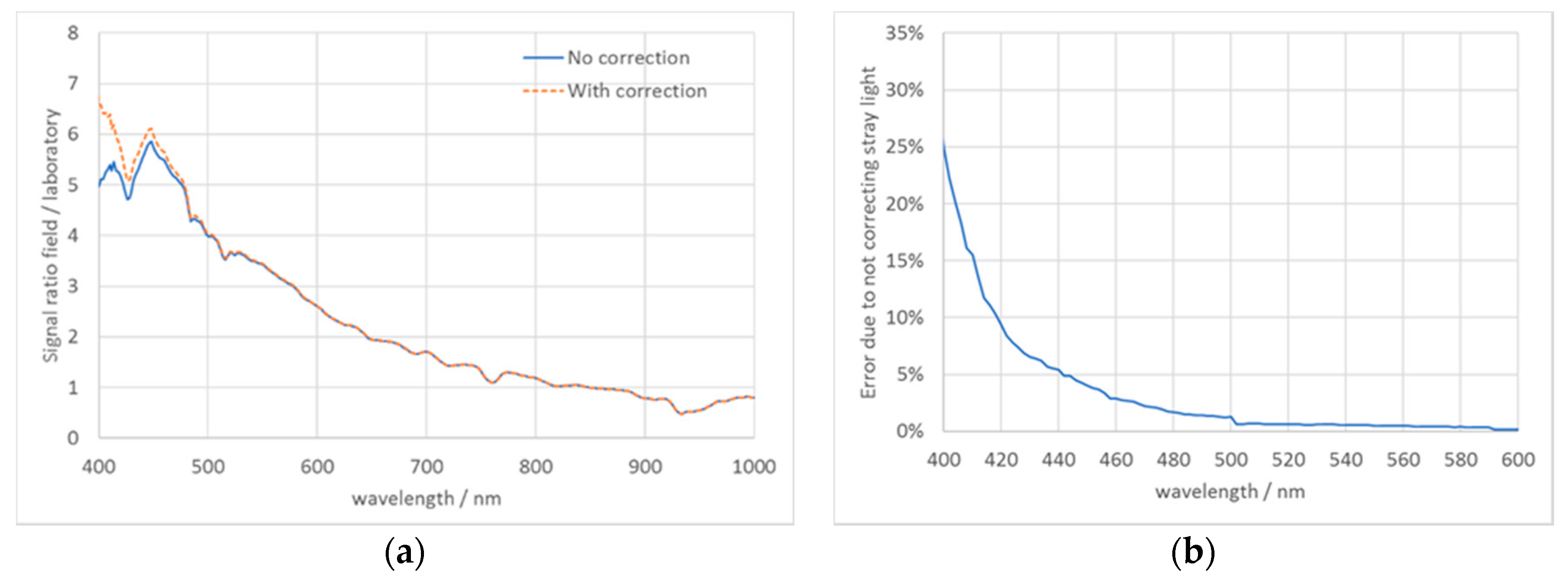
Appendix B. Stray Light Effects

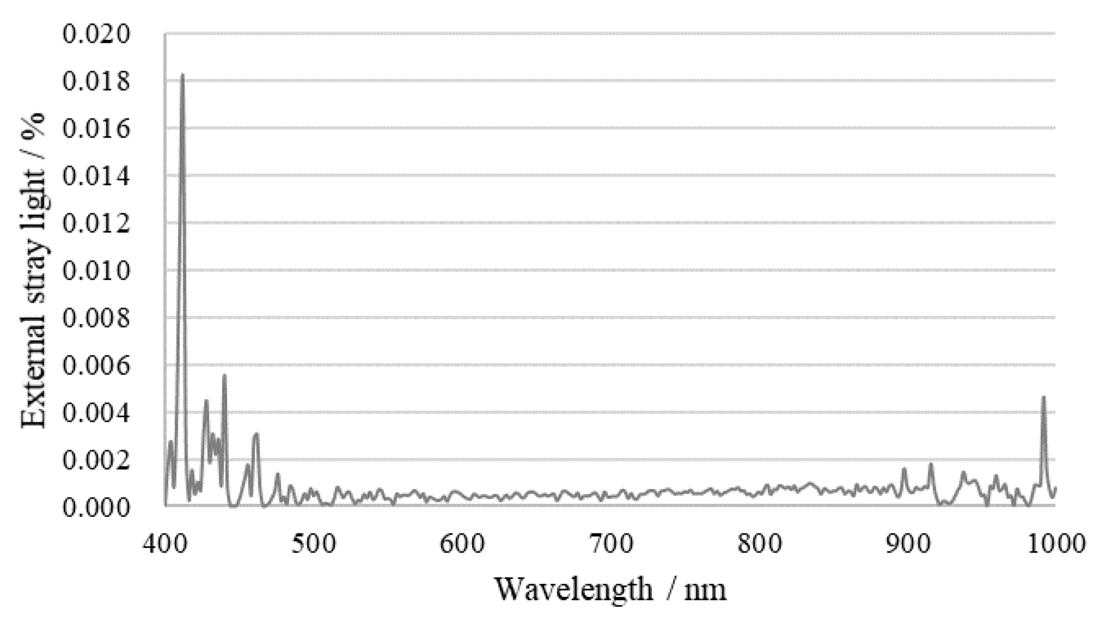
Appendix B.1. External Stray Light during Calibration

The stray light during calibration includes both light that reaches the diffuser panel having scattered off a surface (e.g., walls, optical bench), and light that enters the spectrometer from angles outside its field of view. In the field, it includes light that enters the spectrometer from larger angles. Because the field source is very large (the ground extends in all directions), while in the laboratory the bright panel is surrounded by a dark laboratory, this creates differences between calibration and use. Stray light illuminating the diffuser panel in the laboratory was estimated by blocking the direct beam from the lamp using a small screen and seeing the signal on the spectrometer with and without this beam block. The signal with the block, as a percentage of the signal without the block, is given in Figure A2.
Figure A2. Stray light during calibration as a percentage of the measured signal.
Remotesensing 12 01696 g0a2
The results in Figure A2 show that external stray light is small during calibration (less than ~0.1). When the instrument is used in the field, the stray light signal will be much higher because the surrounding area is brightly illuminated.
For now, we consider an uncertainty associated with external stray light to be 0.1%, recognizing that this is a rough estimate. Further tests are required with sources of differing sizes and with in-the-field stray light testing in order to refine this estimate.

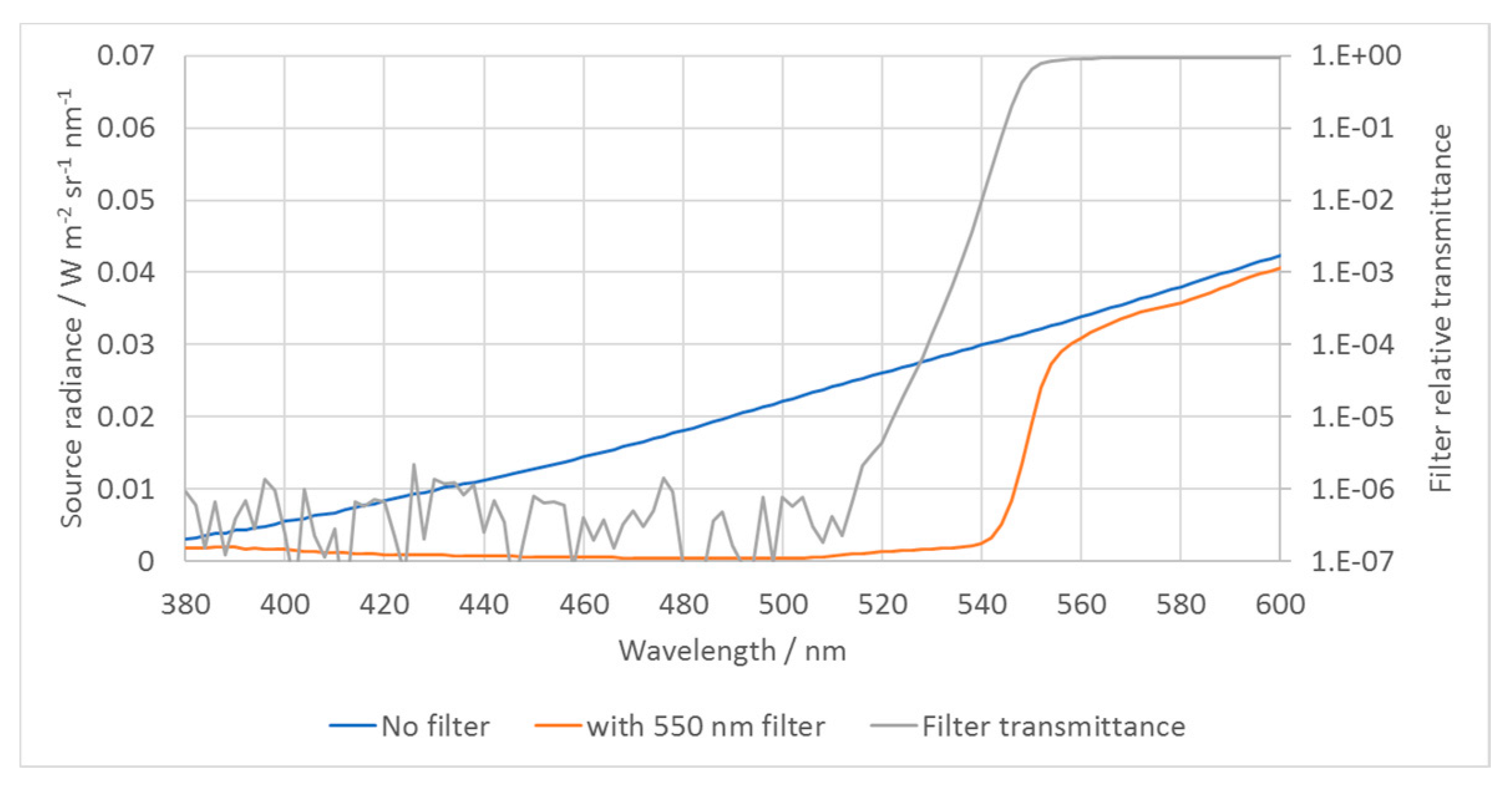
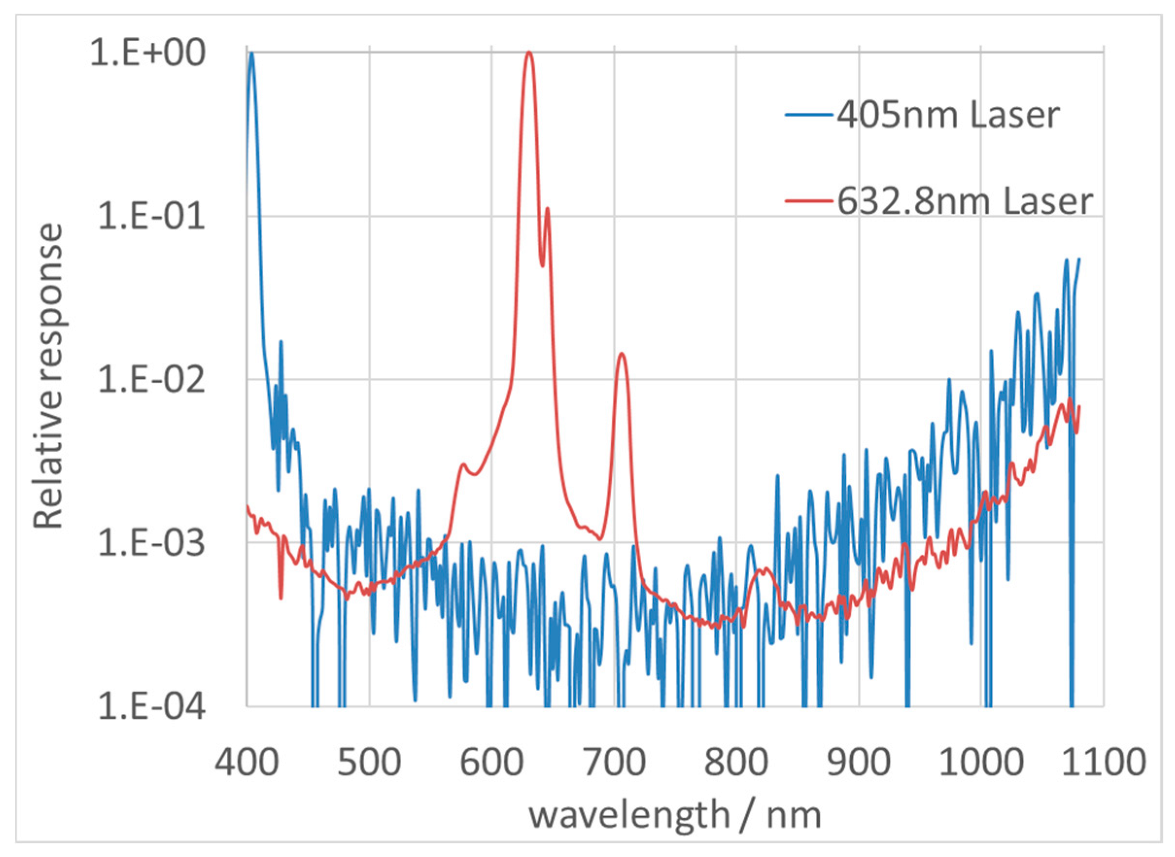
Appendix B.2. Internal (Spectral) Stray Light

Internal stray light is light that scatters within the spectrometer and therefore reaches a spectrometer pixel for the “wrong” wavelength. This is particularly problematic at short wavelengths where the desired signal is small and the detector has a higher sensitivity to light of longer wavelengths than it does to light of the desired wavelength. These two effects combine to mean that a small fraction of light from the much higher radiance longer wavelengths can significantly impact the measured signal at short wavelengths.
This internal spectral stray light was estimated using long-pass filters, which do not transmit light below a cut-on wavelength and have a high transmittance for longer wavelengths. The signal with the filter was compared to the signal without the filter for the shorter wavelengths. Figure A3 shows the signal with and without a 550 nm cut-on filter. At the shortest wavelengths (below 440 nm), the signal with a filter rises and is almost half of the (low) signal with a filter.
Figure A3. Source measured radiance with and without a 550 nm cut on a filter (left vertical axis) and the transmittance of that filter (right vertical axis, logarithmic scale).
Remotesensing 12 01696 g0a3

Appendix B.2.1. Correction for Internal Stray Light

In order to evaluate the impact of this internal stray light, and if necessary to correct for it, we need to determine the effect of this stray light both on the field observations and on the calibration. We define:
V nf , source ( λ ) : Signal (V for volts, but probably actually digital numbers) with no filter of the source.
V f , source ( λ ) : Signal with a filter and the source.
V true , source ( λ ) : The signal that would be measured if the instrument had no stray light response.
τ f ( λ ) : Transmittance of filter.
λ : Wavelength (general concept).
: Wavelength (of a short wavelength pixel that is sensitive to the stray light).
λ min : The shortest wavelength that is considered “long wavelength”.
s ( ) : The fraction of the long wavelength light that makes it to pixel .
Therefore, the measured signal at short wavelength for the calibration source, without a filter is:
V nf , cal ( ) = V true , cal ( ) + s ( ) λ min 1100   nm V true , cal ( λ )   d λ
The measured signal at short wavelength for the calibration source, with a filter is:
V f , cal ( ) = V true , cal , f ( ) + s ( ) λ min 1100   nm τ f ( λ )   V true , cal ( λ )   d λ .
However, since with the filter the “true” signal should be zero, this becomes:
V f , cal ( ) = 0 + s ( ) λ min 1100   nm τ f ( λ )   V true , cal ( λ )   d λ .
Therefore, we can use the calibration with the filter to estimate s ( λ ) :
s ( ) = V f , cal ( ) λ min 1100   nm τ f ( λ )   V true , cal ( λ )   d λ .
In practice, we get the top line from the measurement at the shorter wavelength and the bottom line from integrating the measured signal at longer wavelengths (as we assume there is no stray light in the longer wavelength signal).
A correction can then be applied for any spectral observation (again making the assumption that the longer wavelength signal is insensitive to stray light). Thus, the corrected signal in the field can be calculated from the measured signal at longer wavelengths and the s ( ) determined in the laboratory as:
V true , field ( ) = V nf , field ( ) s ( ) λ min 1100   nm V true , field ( λ )   d λ .

Appendix B.2.2. Experimental Values

The method described in the previous section was applied to one of the spectrometers that are used in the field. The 550 nm cut-on filter results were used to evaluate s ( ) for wavelengths up to 500 nm and the 650 nm cut-on filter for wavelengths from 502 to 590 nm. A 780 nm cut-on filter was used from 592 to 710 nm and a 900 nm cut-on filter for wavelengths from 712 to 870 nm. Wavelengths above 870 nm were not corrected.
The stray light signal, as a percentage of the measured signal, is given in Figure A4, along with the measured source radiance levels. The stray light is less significant in the field than in the laboratory because in the field the radiance at long wavelengths is a similar magnitude to that at short wavelengths, while in the laboratory the source is considerably brighter at longer wavelengths.
Figure A4. (a) Stray light signal as a percentage of the measured signal for both calibration and for a typical in field radiance at BTCN. (b) Source radiance levels.
Remotesensing 12 01696 g0a4
Because the calibration source is used to evaluate the instrument gain and then the instrument gain is multiplied by the in-field observation, the critical quantity to evaluate is the ratio between the field and laboratory measurements with and without stray light correction. Figure A5 shows this ratio with and without correction and the error introduced if the correction is not made.
Figure A5. (a) Ratio of the signal between the field measurement and the laboratory calibration with and without stray light correction. (b) Error introduced if the stray light is not corrected (this is the ratio of the two lines in the left-hand graph).
Remotesensing 12 01696 g0a5

Appendix B.3. More Sophisticated Stray Light Correction

The stray light error is very high for wavelengths below ~450 nm. In order to improve the uncertainty for short wavelengths, this should be corrected. While the method above suggests a possible correction, the uncertainty associated with the correction is difficult to evaluate and likely to be at least half of the correction. Furthermore, the cut-on filter method cannot account for stray light from shorter wavelengths to longer wavelengths.
An improved method for stray light correction is given in Zong et al. [25]. This method involves using a tunable laser to evaluate a stray light correction matrix that can then be applied to the measured signal. Others have shown that this correction only needs to be evaluated once because the correction is stable and also that it is very similar for spectrometers of the same type [26]. It is also possible to combine stray light and bandwidth correction through a single matrix calculation [27]. Salim et al. [28] showed that the method can also be performed using a monochromator when tunable lasers are not available.
It has not yet been possible to perform the necessary spectral measurements with a tunable laser for the BTCN and BSCN spectrometers. However, initial results were obtained with two lasers and are shown in Figure A6. These results show that the shape of the stray light changes with wavelength of the source (and therefore measurements are required for more laser wavelengths) and that there is stray light at longer wavelengths as well as at shorter wavelengths.
Figure A6. Relative response on each pixel (relative to central wavelength response) to a monochromatic 632.8 nm laser and a monochromatic 405 nm laser.
Remotesensing 12 01696 g0a6

Appendix C. Uncertainty Budget

Table A1. Uncertainty budget for BTCN and BSCN BOA reflectance. The abbreviations FC, PC, and I mean fully correlated, partially correlated, and independent, respectively.
EffectError CorrelationUncertainty Magnitude (%)
All Measurements of a Single SpectrometerBetween SpectrometersBetween Wavelengths400 nm500 nm600 nm700 nm800 nm900 nm1000 nm
Lamp Irradiance CalibrationFCFCPC0.420.350.310.290.290.300.31
Lamp Ageing and Current SettingFCPCFC0.290.230.200.170.170.290.32
Diffuser CalibrationFCFCPC0.280.280.280.290.310.320.32
Lamp-Diffuser DistanceFCIFC0.200.200.200.200.200.200.20
Lamp-Diffuser AlignmentFCIFC0.500.500.500.500.500.500.50
Source Non-UniformityFCFCFC0.290.290.290.290.290.290.29
Wavelength AccuracyFCIPC5.001.51.501.501.501.505.00
Spectrometer NoiseIII0.100.100.100.100.100.100.10
Spectrometer NonlinearityFCIFC0.600.370.280.280.280.380.60
Internal Stray LightFCIFC251.300.200.100.100.100.10
External Stray LightFCFCFC0.100.100.100.100.100.100.10
Calibration RepeatabilityFCIFC0.120.150.240.340.460.580.79
Noise during Field MeasurementIII0.410.190.120.110.190.200.28
Spectrometer Temperature SensitivityFCIPC3.380.250.230.300.540.961.97
Solar Irradiance ModelIFCFC1.501.351.050.951.051.050.95
MODTRANPCFCFC2.002.002.002.002.002.002.00
AOTPCFCFC0.280.230.200.170.160.150.13
WVCPCFCFC0.100.100.030.180.120.840.03
Aerosol ModelPCFCFC0.190.080.220.430.470.390.40
Representativeness of the Point Measurement (BTCN)FCIFC5.425.545.485.605.655.715.52
Representativeness of the Point Measurement (BSCN)FCIFC4.093.763.523.453.423.503.67

References

  1. Slater, P.N.; Biggar, S.F.; Holm, R.G.; Jackson, R.D.; Mao, Y.; Moran, M.S.; Palmer, J.M.; Yuan, B. Reflectanceand radiance-based methods for the in-flight absolute calibration of multi-spectral sensors. Remote Sens. Environ. 1987, 22, 11c37. [Google Scholar] [CrossRef]
  2. Meygret, A.; Santer, R.; Berthelot, B. ROSAS: A robotic station for atmosphere and surface characterization dedicated to on-orbit calibration. In Proceedings of the Earth Observing Systems XVI, San Diego, CA, USA, 13 September 2011. [Google Scholar]
  3. Thome, K.J.; Catrall, C.; Amico, J.D.; Geis, J. Ground-reference calibration results for Landsat-7 ETM+. In Proceedings of the SPIE Conference #5882, Earth Observing Systems X, San Diego, CA, USA, 31 July–4 August 2005. [Google Scholar]
  4. Bouvet, M.; Thome, K.; Berthelot, B.; Bialek, A.; Czapla-Myers, J.; Fox, N.P.; Goryl, P.; Henry, P.; Ma, L.; Marcq, S.; et al. RadCalNet: A Radiometric Calibration Network for Earth Observing Imagers Operating in the Visible to Shortwave Infrared Spectral Range. Remote Sens. 2019, 11, 2401. [Google Scholar] [CrossRef] [Green Version]
  5. RadCalNet Portal. Available online: www.radcalnet.org (accessed on 25 May 2020).
  6. QA4EO Portal. Available online: www.qa4eo.org (accessed on 25 May 2020).
  7. JCGM. GUM 2008 JCGM 100:2008. Guide to the Expression of Uncertainty in Measurement (JCGM); BIPM: Sevres, France, 2008; p. 100. Available online: www.bipm.org (accessed on 25 May 2020).
  8. Li, C.; Ma, L.L.; Gao, C.X.; Wang, N.; Liu, Y.K.; Zhang, D.D.; Tang, L.; Liu, X.; Zhao, Y.; Dou, S. Permanent target for optical payload performance and data quality assessment: Spectral characterization and a case study for calibration. J. Appl. Remote Sens. 2014, 8, 083498. [Google Scholar] [CrossRef]
  9. Holben, B.N.; Eck, T.F.; Slutsker, I.; Tanré, D.; Buis, J.P.; Setzer, A.; Vermote, E.; Reagan, J.A.; Kaufman, Y.J.; Nakajima, T.; et al. Aeronet—A federated instrument network and data archive for aerosol characterization. Remote Sens. Environ. 1998, 66, 1–16. [Google Scholar] [CrossRef]
  10. AERONET Website. Available online: https://aeronet.gsfc.nasa.gov/ (accessed on 25 May 2020).
  11. Mittaz, J.; Merchant, C.J.; Woolliams, E.R. Applying principles of metrology to historical Earth observations from satellites. Metrologia 2019, 56, 032002. [Google Scholar] [CrossRef]
  12. Berk, A.; Anderson, G.P.; Acharya, P.K.; Chetwynd, J.H.; Borel, C.C.; Lewis, P.E. Modtran 5: A reformulated atmospheric band model with auxiliary species and practical multiple scattering options: Update. In Proceedings of the SPIE, the International Society for Optical Engineering, Boston, MA, USA, 23–25 OCtober 2005; Volume 5806, pp. 662–667. [Google Scholar]
  13. Schaepman-Strub, G.; Schaepman, M.E.; Painter, T.H.; Dangel, S.; Martonchik, J.V. Reflectance quantities in optical remote sensing—Definitions and case studies. Remote Sens. Environ. 2006, 103, 27–42. [Google Scholar] [CrossRef]
  14. Dai, C.H.; Khlevnoy, B.; Wu, Z.F.; Wang, Y.F.; Li, L.L. Bilateral comparison of spectral irradiance between NIM and VNIIOFI from 250 to 2500 nm. MAPAN 2017, 32, 243–250. [Google Scholar] [CrossRef]
  15. Thuillier, G.; Hersé, M.; Labs, D.; Foujols, T.; Peetermans, W.; Gillotay, D.; Simon, P.C.; Mandel, H. The solar spectral irradiance from 200 to 2400 nm, as measured by the SOLSPEC spectrometer from the Atlas and Eureca Missions. Sol. Phys. 2003, 214, 1–22. [Google Scholar] [CrossRef]
  16. Barbrow, L.E. International Lighting Vocabulary. J. Smpte 1964, 73, 331–332. [Google Scholar] [CrossRef]
  17. Salim, S.; Fox, N.; Theocharous, E.; Sun, T.; Grattan, T.V. Temperature and nonlinearity corrections for a photodiode array spectrometer used in the field. Appl. Opt. 2011, 50, 866–875. [Google Scholar] [CrossRef] [PubMed]
  18. Reagan, J.A.; Thome, K.; Herman, B.; Gall, R. Water vapor measurements in the 0.94 micron absorption band—Calibration, measurements and data applications. J. Mol. Spectrosc. 2015, 68, 329–330. [Google Scholar]
  19. Sinyuk, A.; Holben, B.N.; Smirnov, A.; Eck, T.F.; Slutsker, I.; Schafer, J.S.; Giles, D.M.; Sorokin, M. Assessment of error in aerosol optical depth measured by AERONET due to aerosol forward scattering. Geophys. Res. Lett. 2012, 39, L23806. [Google Scholar] [CrossRef]
  20. Berk, A.; Anderson, G.P.; Acharya, P.K. MODTRAN® 5.2. 2 User’s Manual 2011; Spectral Sciences Inc.: Burlington, MA, USA, 2011; Volume 69. [Google Scholar]
  21. Thuillier, G.; Hersé, M.L.; Simon, P.C.; Labs, D.; Mandel, H.; Gillotay, D.; Foujols, T. The visible solar spectral irradiance from 350 to 850 nm as measured by the SOLSPEC spectrometer during the atlas I mission. Sol. Phys. 1998, 177, 41–61. [Google Scholar] [CrossRef]
  22. Otterman, J.; Fraser, R.S. Adjacency effects on imaging by surface reflection and atmospheric scattering: Cross radiance to zenith. Appl. Opt. 1979, 18, 2852–2860. [Google Scholar] [CrossRef] [PubMed]
  23. Ma, L.L.; Wang, N.; Zhao, Y.G.; Liu, Y.K.; Han, Q.J.; Wang, X.H.; Woolliams, E.R.; Gao, C.X.; Bouvet, M.; Li, C.R.; et al. An improved vicarious radiometric calibration method considering the adjacency effect for high Resolution optical sensors. IEEE Trans. Geosci. Remote Sens. 2019. under-review. [Google Scholar]
  24. Gorroño, J.; Hunt, S.; Scanlon, T.; Banks, A.; Fox, N.; Woolliams, E.R.; Underwood, C.; Gascon, F.; Peters, M.; Fomferra, N.; et al. Providing uncertainty estimates of the Sentinel-2 top-of-atmosphere measurements for radiometric validation activities. Eur. J. Remote Sens. 2018, 51, 650–666. [Google Scholar] [CrossRef] [Green Version]
  25. Zong, Y.Q.; Brown, S.W.; Johnson, B.C.; Lykke, K.R.; Ohno, Y. Simple spectral stray light correction method for array spectroradiometers. Appl. Opt. 2006, 45, 1111–1119. [Google Scholar] [CrossRef] [PubMed]
  26. Nevas, S.; Sperling, A.; Oderkerk, B. Transferability of stray light corrections among array spectroradiometers. AIP Conf. Proc. 2013, 1531, 821–824. [Google Scholar]
  27. Nevas, S.; Wübbeler, G.; Sperling, A.; Elster, C.; Teuber, A. Simultaneous correction of bandpass and stray-light effects in array spectroradiometer data. Metrologia 2012, 49, S43. [Google Scholar] [CrossRef]
  28. Salim, S.G.R.; Fox, N.P.; Hartree, W.S.; Woolliams, E.R.; Sun, T.; Grattan, K.T.V. Stray light correction for diode-array-based spectrometers using a monochromator. Appl. Opt. 2011, 50, 5130–5138. [Google Scholar] [CrossRef] [PubMed]
Figure 1. (a) The satellite image of the Baotou site; (b) the reflectance of BTCN and BSCN sites.
Remotesensing 12 01696 g001
Figure 2. Automatic observation systems of ground reflected radiance in the Baotou site. (a) Observation system on grey target; (b) observation system on sandy site; (c) the positions of the two spectrometers on sandy site.
Remotesensing 12 01696 g002
Figure 3. Light paths for radiation from the site (simplified to ignore multiple scattering).
Remotesensing 12 01696 g003
Figure 4. Uncertainty tree diagram for the Baotou measurements of ground spectral reflectance.
Remotesensing 12 01696 g004
Figure 5. Error in the ratio of the field to laboratory measurement (proxy for error in the true field measurement) due to not correcting for wavelength.
Remotesensing 12 01696 g005
Figure 6. Nonlinearity factor obtained for five different radiance levels (radiance levels in legend are in units W m−2 sr−1 nm−1 at 800 nm).
Remotesensing 12 01696 g006
Figure 7. Relative difference in the calibration following realignment and realignment and transportation.
Remotesensing 12 01696 g007
Figure 8. Empirically fitted temperature corrections as a function of wavelength.
Remotesensing 12 01696 g008
Figure 9. Residual from the measurements to the fit model at different wavelengths. The black curve gives the assumed uncertainty associated with the model (the plus-zero term in Equation (5)).
Remotesensing 12 01696 g009
Figure 10. Uncertainty associated with downwelling irradiance (sun and sky) caused by a relative measurement uncertainty of 12% in the water vapor column (WVC).
Remotesensing 12 01696 g010
Figure 11. Uncertainty associated with downwelling irradiance (sun and sky) caused by a measurement uncertainty of 0.01 in the aerosol optical depth (AOD).
Remotesensing 12 01696 g011
Figure 12. Relative difference between the calculated total downwelling irradiance for a real data set at Baotou assuming a desert model and a rural model.
Remotesensing 12 01696 g012
Figure 13. The combined uncertainty associated with ground reflectance.
Remotesensing 12 01696 g013
Figure 14. Uncertainty associated with the BOA reflectance.
Remotesensing 12 01696 g014
Figure 15. Difference of top-of-atmosphere (TOA) reflectance between correcting and not correcting for background adjacency effect for BTCN and BSCN targets.
Remotesensing 12 01696 g015
Figure 16. The combined uncertainty associated with propagation to top-of-atmosphere reflectance.
Remotesensing 12 01696 g016
Table 1. Uncertainties associated with reference source radiance.
EffectLamp Irradiance CalibrationLamp Ageing and Current SettingDiffuser CalibrationLamp-Diffuser DistanceLamp-Diffuser AlignmentSource Non-Uniformity
Term affected E FEL ( λ i ) in Equation (2) E FEL ( λ i ) in Equation (2) β ( λ i ) in Equation (2) + 0 in Equation (2) + 0 in Equation (2) + 0 in Equation (2)
Error correlationAll measurements of a single spectrometerFully correlatedFully correlatedFully correlatedFully correlatedFully correlatedFully correlated
Between spectrometersFully correlatedPartially correlated 1Fully correlatedIndependentIndependentFully correlated 2
Between wavelengthsPartially correlated 1Fully correlatedPartially correlated 3Fully correlatedFully correlatedFully correlated
Uncertainty magnitude400 nm0.42%0.29%0.28%0.20%0.50%0.29%
500 nm0.35%0.23%0.28%0.20%0.50%0.29%
600 nm0.31%0.20%0.28%0.20%0.50%0.29%
700 nm0.29%0.17%0.29%0.20%0.50%0.29%
800 nm0.29%0.17%0.31%0.20%0.50%0.29%
900 nm0.30%0.29%0.32%0.20%0.50%0.29%
1000 nm0.31%0.32%0.32%0.20%0.50%0.29%
1 Lamp ageing is likely to have an error that is fully correlated between spectrometers as long as the lamp is not operated for a long time between the two spectrometer calibrations. Current setting is independent between spectrometers as it is dominated by short term effects. 2 Source non-uniformity is dominated by effects that are common for all calibrations as the spatial distribution stays basically constant for all alignments and the spectrometers have near identical fields of view. 3 The lamp irradiance calibration and the diffuser calibration were performed on NIM’s primary facilities. The uncertainty budget for that has components that are fully correlated between wavelengths and components that are independent between wavelengths.
Table 2. Uncertainties associated with laboratory calibration of the spectrometer.
EffectSource RadianceWavelength AccuracySpectrometer Noise
Term affected L source ( λ i ) in Equation (2) λ i in Equation (2) C cal ( λ i ) in Equation (2)
Error correlationAll measurements of a single spectrometerMixed. See Table 1Fully correlatedIndependent
Between spectrometersMixed. See Table 1IndependentIndependent
Between wavelengthsMixed. See Table 1Partially correlatedIndependent
Uncertainty magnitude400 nm0.84%5.00%0.10%
500 nm0.79%1.50%0.1 0%
600 nm0.77%1.50%0.10%
700 nm0.76%1.50%0.10%
800 nm0.76%1.50%0.10%
900 nm0.81%1.50%0.10%
1000 nm0.82%5.0%0.10%
Spectrometer NonlinearityInternal Stray LightExternal Stray LightCalibration Repeatability
+ 0 in Equation (2) + 0 in Equation (2) + 0 in Equation (2) + 0 in Equation (2)
Error correlationFully correlatedFully correlatedFully correlatedFully correlated
IndependentIndependentFully correlatedIndependent
Fully correlatedFully correlatedFully correlatedFully correlated
Uncertainty magnitude0.60%25%0.10%0.12%
0.37%1.30%0.10%0.15%
0.28%0.20%0.10%0.24%
0.28%0.10%0.10%0.34%
0.28%0.10%0.10%0.46%
0.38%0.10%0.10%0.58%
0.60%0.10%0.10%0.79%
Table 3. The uncertainty associated with field radiance measured by the spectrometer.
EffectLaboratory CalibrationNoise During Field MeasurementSpectrometer Temperature Sensitivity
Term affected G ( λ i ) in Equation (4) C cal ( λ i ) in Equation (4) f ( λ i , T ) in Equation (4)
Error correlationAll measurements of a single spectrometerMixed. See Table 2IndependentFully correlated
Between spectrometersMixed. See Table 2IndependentIndependent
Between wavelengthsMixed. See Table 2IndependentPartially correlated 1
Uncertainty magnitude400 nm25.43%0.41%3.38%
500 nm2.16%0.19%0.25%
600 nm1.74%0.12%0.23%
700 nm1.75%0.11%0.30%
800 nm1.77%0.19%0.54%
900 nm1.85%0.2%0.96%
1000 nm5.16%0.28%1.97%
1 The error due to temperature sensitivity is partly correlated from wavelength to wavelength. The component that relates to uncertainty in the model is independent, while the component that is from the propagation of temperature uncertainty to radiance uncertainty is fully correlated.
Table 4. The uncertainty associated with ground reflectance measured by the spectrometer.
EffectField RadianceSolar Irradiance ModelMODTRANAOTWVCAerosol Model
Term affected L gnd ( λ i , t ) in Equation (1) E sun ( θ , d ; λ i ) + E sky ( λ i , t ) in Equation (1)
Error correlationAll measurements of a single spectrometerMixed. See Table 3Partially correlatedPartially correlatedPartially correlatedPartially correlatedPartially correlated
Between spectrometersMixed. See Table 3Fully correlatedFully correlatedFully correlatedFully correlatedFully correlated
Between wavelengthsMixed. See Table 3Fully correlatedFully correlatedFully correlatedFully correlatedFully correlated
Uncertainty magnitude400 nm25.66%1.50%2.00%0.28%0.10%0.19%
500 nm2.18%1.35%2.00%0.23%0.10%0.08%
600 nm1.76%1.05%2.00%0.20%0.03%0.22%
700 nm1.78%0.95%2.00%0.17%0.18%0.43%
800 nm1.86%1.05%2.00%0.16%0.12%0.47%
900 nm2.09%1.05%2.00%0.15%0.84%0.39%
1000 nm5.53%0.95%2.00%0.13%0.03%0.40%

