Article

Spatial-Adaptive Siamese Residual Network for Multi-/Hyperspectral Classification

1
Guangdong Provincial Key Laboratory of Urbanization and Geo-Simulation, Center of Integrated Geographic Information Analysis, Southern Marine Science and Engineering Guangdong Laboratory (Zhuhai), School of Geography and Planning, Sun Yat-sen University, Guangzhou 510275, China
2
City College of Dongguan University of Technology, Dongguan 511700, China
*
Author to whom correspondence should be addressed.
Remote Sens. 2020, 12(10), 1640; https://doi.org/10.3390/rs12101640
Submission received: 12 April 2020 / Revised: 12 May 2020 / Accepted: 16 May 2020 / Published: 20 May 2020

Abstract

:
Deep learning methods have been successfully applied for multispectral and hyperspectral images classification due to their ability to extract hierarchical abstract features. However, the performance of these methods relies heavily on large-scale training samples. In this paper, we propose a three-dimensional spatial-adaptive Siamese residual network (3D-SaSiResNet) that requires fewer samples and still enhances the performance. The proposed method consists of two main steps: construction of 3D spatial-adaptive patches and Siamese residual network for multiband images classification. In the first step, the spectral dimension of the original multiband images is reduced by a stacked autoencoder and superpixels of each band are obtained by the simple linear iterative clustering (SLIC) method. Superpixels of the original multiband image can be finally generated by majority voting. Subsequently, the 3D spatial-adaptive patch of each pixel is extracted from the original multiband image by reference to the previously generated superpixels. In the second step, a Siamese network composed of two 3D residual networks is designed to extract discriminative features for classification and we train the 3D-SaSiResNet by pairwise inputting the training samples into the networks. The testing samples are then fed into the trained 3D-SaSiResNet and the learned features of the testing samples are classified by the nearest neighbor classifier. Experimental results on three multiband image datasets show the feasibility of the proposed method in enhancing classification performance even with limited training samples.

Graphical Abstract

1. Introduction

Remote sensing [1,2,3,4] has played an important role in Earth observation problems. The ever-growing number of multispectral and hyperspectral images acquired by satellite sensors facilitates a deeper understanding of the Earth’s environment and human activities. Rapid advances in remote sensing technology and computing power have contributed to the application of multiband images in environmental monitoring [5], land-cover mapping [6,7], and anomaly detection [8]. Classification, which labels each pixel with a specific land-cover type, is one of the fundamental tasks in remote sensing analysis [9,10,11]. A large number of labeled training data are usually required to achieve satisfactory classification performance. However, it is time-consuming and expensive to label the remote sensing samples in practice.
In the remote sensing community, researchers have proposed various supervised approaches to classify the multiband images. Existing methods can be roughly divided into two categories. The first category is spectral classification methods, which classify each pixel independently by utilizing the spectral features. State-of-the-art methods include the support vector machine (SVM) [12] and its variations [13,14]. Although the spectral methods have proven to be useful for multiband images classification, they fail to fully explore the spatial information, and therefore result in salt and pepper-like errors. The second category is spectral-spatial classification methods, which use both spectral and spatial information for more accurate classification performance. In this category, additional spatial features extracted by diverse strategies are integrated into the pixel-wise classifiers. Widely-used spatial extraction methods include the morphological profiles [15], attribute profiles [16], gray-level cooccurrence matrix [17], Gabor transform [18], and wavelet transform [19]. Image segmentation can also be applied to obtain the spatial neighbors. For instance, superpixel segmentation groups pixels of multiband images into perceptually meaningful atomic regions which are more flexible than the rigid square patches [20,21]. Many classifiers are also proposed for spectral-spatial classification, such as the joint sparsity model (JSM) [22], multiple kernel learning (MKL) [23], and Markov random field (MRF) modeling [24]. Moreover, note that the remote sensing images can be modeled as three-dimensional (3D) cubes with one spectral dimension and two spatial dimensions. Researchers have developed some spectral-spatial methods under the umbrella of tensor theory, such as the tensor discriminative locality alignment (TDLA) method [25], tensor block-sparsity based representation [26], and local tensor discriminative analysis technique (LTDA) [27]. Spectral-spatial methods have proved to be more effective than the spectral methods as they can exploit the object shape, size, and textural features from the multiband images.
However, most of the above-mentioned methods cannot classify the multiband images in a “deep” fashion. In recent years, deep learning [28,29,30,31] has attracted extensive attention with the rapid development of artificial intelligence. Deep learning can hierarchically learn the high-level features, and therefore has achieved tremendous success in remote sensing classification. Typical deep architectures include the stacked autoencoder (SAE) [32], deep belief network (DBN) [33], residual network (ResNet) [34], and generative adversarial network (GAN) [35]. Among all deep learning-based methods being developed over the past few years, convolutional neural networks (CNNs) have become a preferable model in the current trend of multiband images analysis due to the fact that convolutional filters are powerful tools to automatically extract the spectral-spatial features. For instance, a one-dimensional CNN (1D-CNN) method was proposed in [36] for hyperspectral classification in the spectral domain. A spectral-spatial classification method was proposed in [37] by combining the principle component analysis (PCA), two-dimensional CNN (2D-CNN), and logistic regression. [38] improved the performance of remote sensing image scene classification by imposing a metric learning regularization term on the CNN features. The 3D-CNN was applied in [39] to learn the local signal changes in spectral-spatial dimension of the 3D cubes, while [40] explored the performance of deep learning architectures for remote sensing classification and introduced a 3D deep architecture by applying 3D convolution operations instead of using 1D convolution operations. In [41], residual blocks connected every 3D convolutional layer by identity mapping to gain improved classification performance. Moreover, the Siamese networks [42] composed of 2D-CNN/3D-CNN or 2D-ResNet/3D-ResNet [43,44,45,46] were also proposed for hyperspectral classification. The Siamese architecture differs from other deep learning-based methods in that it is directly trained to separate the similar pairs from the dissimilar in feature space. By simultaneously learning the similarity metrics, the Siamese networks are effective for distinguishing different land-covers in remote sensing data. However, all those Siamese networks performed pixel-based classification of hyperspectral data by choosing the neighborhoods of a sample as the original features. Although CNN and its variations have been successfully employed in classification of multiband images, training, or testing samples are usually fixed at the center of the neighborhood windows and the neighboring samples in each patch are assumed to be consisted of similar materials. However, in heterogeneous regions, especially around the boundaries, neighboring samples often belong to different classes, which go against the basic assumption of the deep learning-based methods.
In this paper, we propose a 3D spatial-adaptive Siamese residual network (3D-SaSiResNet) for classification of multiband images. The main steps of the proposed method are twofold, i.e., construction of 3D spatial-adaptive patches and Siamese residual network for multiband images classification. In the first step, we segment the multiband images into spatial-adaptive patches instead of choosing the patches centered on training/testing samples. In the second step, we design a 3D-SaSiResNet to extract high-level features for classification. The 3D-SaSiResNet is composed of two 3D ResNet channels with shared weights and the training samples are utilized to train the network in pairs. The testing samples are then fed into the trained Siamese network to obtain the learned features, which can be classified by the nearest neighbor classifier. The two steps are closely connected, i.e., in the first step, we generate 3D spatial-adaptive patches, which can be subsequently classified by the 3D-SaSiResNet built in the second step.
The main contributions of this work are listed below:
  • We obtain 3D spatial-adaptive patches of the multiband images by band reduction and superpixel segmentation. Instead of fixing the samples at the center of the patches, the 3D spatial-adaptive patches provide a more flexible way to fully consider the heterogeneous regions of the remote sensing data, making the neighbors within the same 3D patch more probable to have the same class label.
  • We propose a 3D-SaSiResNet method for classification of multiband images. The Siamese architecture of the network combined with 3D ResNet helps to extract discriminative spectral-spatial features from the remote sensing data cube and provides promising classification performance even with limited training samples.
The rest of this paper is organized as follows. In Section 2, detailed descriptions of the proposed method are provided. Section 3 reports experimental results on three multiband image datasets and conclusions are drawn in Section 4.

2. Proposed Method

In this section, we provide the detailed procedure of the proposed method, which contains two main parts: construction of 3D spatial-adaptive patches and 3D-SaSiResNet for multiband image classification (see Figure 1). Both parts of the proposed method are important for multiband image classification. First, compared to fixing the training or testing samples at the center of the patches, constructing spatial-adaptive patches can fully follow the spatial characteristics of the multiband image, making the pixels within the same patch more likely to be in the same category. It is notable that the hyperspectral image usually has more than one hundred contiguous bands, and band reduction is also essential to reduce the computational cost in the first steps. Second, the 3D-SaSiResNet facilitates the extraction of discriminant features and classification of multiband images.

2.1. Construction of 3D Spatial-Adaptive Patches

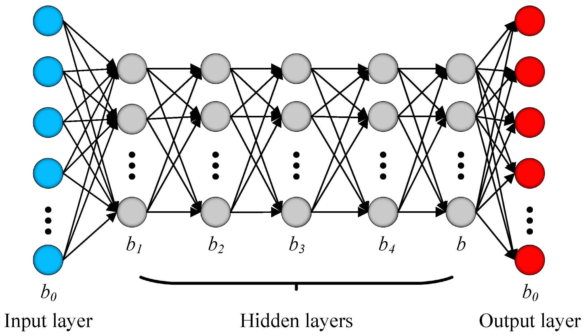
In the proposed method, we segment the multiband images into 3D spatial-adaptive patches, ensuring that the neighbors within the same patch are more likely to consist of the same materials. To reduce the computational cost, band reduction implemented by SAE [31,47,48] is first performed on the original images. The reason for utilizing the SAE for band reduction is that the accuracy of superpixel segmentation results is important for the proposed method and the SAE can provide an effective nonlinear transformation and nonlinear band reduction. Letting I 0 R m 0 × n 0 × b 0 be the original multiband images data, where m 0 , n 0 , and b 0 represent the number of rows, columns, and spectral bands, respectively, the intrinsic dimensionality of I 0 can be estimated by the “intrinsic_dim” function in the “drtoolbox” [49], which is a public MATLAB toolbox for dimensionality reduction. Supposing the intrinsic dimensionality of I 0 is b, we design a SAE network to reduce the band of I 0 from b 0 to b. The structure of the SAE used in this paper is depicted in Figure 2, where the input layer I ˜ 0 R b 0 is the spectral signature of I 0 . As shown in Figure 2, SAE is a stacked structure of multiple autoencoders and each autoencoder is a single hidden layer feedforward network, whose output aims to reconstruct the input signal. In every single autoencoder, the hidden layer units are less in number than the input and output layer units. As such, the autoencoder network learns a compressed representation of the high-dimensional remote sensing data. Without loss of generality, supposing the input signal of a single autoencoder is X R b x , which is reduced to b y features representing high abstraction in the hidden layer, and then the X is reconstructed into Z R b x . The above-mentioned process can be formulated as
Y = f y ( w y X + β y )
Z = f z ( w z Y + β z )
where Y R b y refers to the compressed data in the encoding step, Z represents the reconstructed data in the decoding step, w y and w z denote the weights of input-to-hidden and hidden-to-output, respectively, β y and β z are the bias of the hidden and output units, respectively, and f y ( · ) and f z ( · ) denote the activation functions.
The autoencoder can be trained by minimizing the following reconstruction error:
min w y , w z , β y , β z X Z 2 2
The SAE used in this paper is a stacked series of autoencoders layer by layer, where the hidden layer output of the previous autoencoder is taken as the input of the next layer. The parameters of the SAE can be obtained by training each autoencoder hierarchically with the back propagation algorithm in an unsupervised fashion. Moreover, it is worthwhile to note that we use five hidden layers (the number of units is set to 100, 50, 25, 10, and b, respectively) for band reduction of hyperspectral image since the hyperspectral image usually contains hundreds of contiguous spectral bands, too many layers will increase the computing burden, while fewer layers will reduce the extraction effect. As to the multispectral image, only one hidden layer (the number of units is set to the intrinsic dimensionality) is needed since the spectral bands of multispectral image are usually less than 10, and, therefore, it is not necessary to adopt as many hidden layers as the hyperspectral image has.
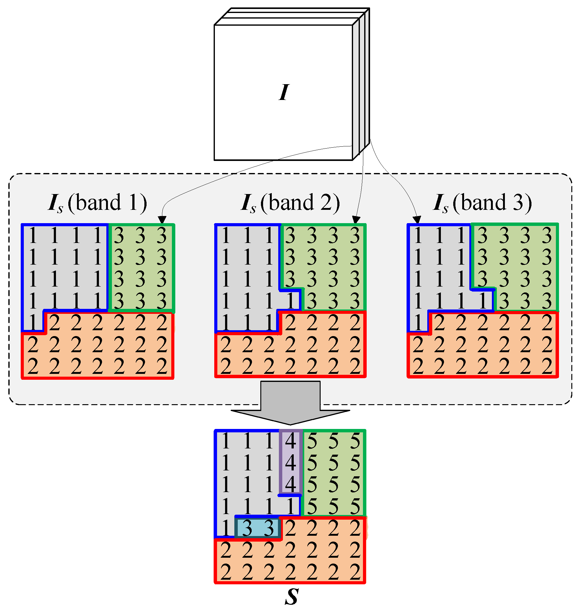
Simple linear iterative clustering (SLIC) [20] is then performed on each of the reduced bands to obtain over-segmented maps. Letting I R m 0 × n 0 × b be the multiband image with reduced bands and I s R m 0 × n 0 × b be the superpixel segmentation results obtained by performing SLIC to each of the b band, the final superpixel map S can be generated by Algorithm 1. Moreover, Figure 3 gives an example about how to obtain S . There are three bands in I , and I s R 7 × 7 × 3 denotes the segmentation results of SLIC. In case the intersection of all the over-segmented regions where the pixel ( p , q ) located is not empty, the pixels located at that intersection will be given the same label. Otherwise, a single label is given to the ( p , q ) th pixel. The above-mentioned procedure is repeated with ( p , q ) changes from ( 1 , 1 ) to ( 7 , 7 ) , and the superpixel map S is finally generated by traversing all of the pixels in I s . Moreover, it is important to note that the labels in S denote different segmentation blocks rather than represent the class labels of land covers.
Given the superpixel map S , instead of fixing a certain sample s 0 at the center, the 3D spatial-adaptive patch of s 0 is determined by cropping the minimum bounding rectangle of the superpixel in which s 0 lies and extracting the pixels from the input multiband image according to the cropped minimum bounding rectangle. To ensure all the pixels in the same patch have the same land-cover class, those pixels, which are located in the minimum bounding rectangle but do not belong to the same superpixel, are substituted by the mean of the rest pixels in the minimum bounding rectangle. All of the 3D patches are resized to the same window size by bicubic interpolation for the convenience of model training. Specifically, Figure 4 depicts a schematic example of the patch generation procedure. The window size of the patch is set to 3 × 3 . Figure 4a denotes the procedure of extracting a 3D patch by fixing a certain sample s 0 at the center, the materials, and land-covers of the neighbors may be quite different from s 0 , and the number of patches is equal to the number of samples. Figure 4b denotes the procedure of extracting a 3D spatial-adaptive patch, in which the neighbors are more likely to have the same labels as s 0 . Moreover, all the pixels that are contained within the same superpixel result in the same 3D spatial-adaptive patch, and, therefore, the number of generated 3D spatial-adaptive patches is equal to the number of superpixels. Taking each 3D spatial-adaptive patch as an object in multiband classification, the 3D-SaSiResNet is, in essence, an object-based method rather than a pixel-based method.
Algorithm 1:Generating the superpixel mapS.
Remotesensing 12 01640 i001

2.2. 3D-SaSiResNet for Multiband Image Classification

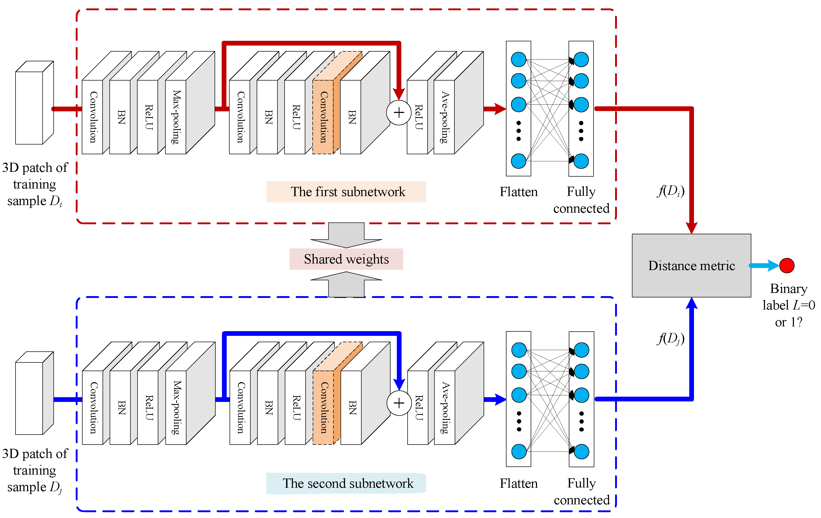
We propose a 3D-SaSiResNet to extract high-level features for supervised classification of the multiband images. Supposing the training set comprises N cases and can be represented by { s i , l i } , i = 1 , 2 , , N , where s i R b 0 refers to the spectral signature of the ith training sample and l i is the class label, the 3D spatial-adaptive patch D i R w × w × b 0 of s i is extracted from the original multiband images data I 0 R m 0 × n 0 × b 0 by reference to the superpixels generated in Section 2.1, where w is the window size of D i . The 3D patches of training samples are grouped in C N 2 = N ( N 1 ) / 2 pairs { D i , D j } , i j , i , j = 1 , 2 , , N , where C N 2 refers to a combination of the N patches in mathematics, and it involves the number of times to select two patches from a set of N patches without repetition. The pairs { D i , D j } are then fed into the two subnetworks of the proposed method. In other words, N ( N 1 ) / 2 pairs of 3D patches are compared when we train the network. The architecture of the 3D-SaSiResNet is illustrated in Figure 5, which contains two identical subnetworks with the same configurations and shared weights. The training procedure aims to train a model to discriminate between a series of pairs from same/different classes. As shown in Figure 5, the first subnetwork takes D i as input, followed by a sequence of 3D convolution [39], 3D batch normalization (3D-BN) [50], 3D rectified linear unit (3D-ReLU) [51], 3D max-pooling [52], and a 3D residual basic block [34] (or 3D ResNeXt basic block [53]) with skip connection, the output of the last pooling layer is flattened as a vector to connect with a fully connected layer, and the last vector f ( D i ) is the features of D i produced by the above-mentioned subnetwork. The second subnetwork takes D j as input, followed by the same procedure as performed in the first subnetwork, and outputs the features f ( D j ) . In greater detail, the five kinds of layers involved in the 3D-SaSiResNet are described in the following:
  • 3D convolution layers: The 3D convolution layers [39] directly take 3D cubes (e.g., 3D patch D i ) as input and are more suitable for simultaneously extracting spectral-spatial features of the multiband images than the 2D ones. Each input 3D feature map of the convolution layer is convolved with a 3D filter and is then passed through an activation function to generate the output 3D feature map
    D h = D h 1 * K h + β h
    where D h 1 and D h are the feature maps of the ( h 1 ) th and hth layers, K h and β h represent the 3D filter and bias in the hth layer, respectively.
  • 3D-BN layers: The 3D-BN layers [50] reduce the internal covariate shift in the network model by normalization, which allows a more independent learning process in each layer. 3D-BN can regularize and accelerate the learning process, imposing a Gaussian distribution on the feature maps. Specifically, letting V be the original batch feature cube, 3D-BN produces the transformed output V ^ by
    V ^ = V M E A N ( V ) V A R ( V ) + ϵ * γ + η
    where M E A N ( · ) and V A R ( · ) are the mean and standard-deviation calculated per-dimension over the mini-batches, respectively, γ and η are learnable parameter vectors, and ϵ > 0 is a small number to prevent numerical instability.
  • ReLU layers: ReLU layers [51] are nonlinear activation functions applied to each element of the feature map to gain nonlinear representations. As a widely-used activation function in neural networks, ReLU is faster than other saturating activation functions. The formula of the ReLU function is
    R e L U ( x ) = max ( 0 , x )
  • 3D pooling layers: 3D pooling layers [52] reduce the data variance and computation complexity by sub-sampling operations, such as max-pooling and average-pooling. The feature maps are first divided into several non-overlapping 3D cubes, and then the maximum or average value within each 3D cube are mapped into the output feature map.
  • 3D residual basic blocks/3D ResNeXt basic blocks: 3D residual basic blocks [34] (or 3D ResNeXt basic blocks [53]) are adopted in the proposed model to alleviate the vanishing/exploding gradient problem. Two types of connections are involved in the 3D residual basic blocks. The first is a feedforward connection that connects layer by layer, i.e., each layer is connected with the former layer and the next layer. The second is the shortcut connection that connects the input with its output and preserves information across layers. The outputs of those two types of connection are summed, followed by a ReLU layer
    D ^ h 1 = I ( D h 1 ) + F ( D h 1 , W h 1 ) D h = R e L U ( D ^ h 1 )
    where D ^ h 1 denotes the sum of the identity mapping I ( D h 1 ) and residual function F ( D h 1 , W h 1 ) , W h 1 is the weight matrix, and D h 1 and D h are the input and output feature maps of the residual basic block. The structure of 3D ResNeXt basic blocks is similar to the 3D residual basic blocks except for substituting the second convolution layer of the 3D residual basic block into grouped convolutions.
Given the features f ( D i ) and f ( D j ) extracted by the first and second subnetworks, the following Euclidean distance is adopted as the metric to compute the distance between D i and D j
E ( D i , D j ) = f ( D i ) f ( D j ) 2
After the architecture of the 3D-SaSiResNet is constructed, we train the model for many epochs using the pairs { D i , D j } , i j , i , j = 1 , 2 , , N . The parameter θ of the 3D-SaSiResNet is updated through minimizing the contrastive loss function Q ( θ )
Q ( θ ) = i = 1 , j = 1 , i j N Q ( θ , ( L , D i , D j ) ) = i = 1 , j = 1 , i j N ( 1 L ) Q S ( E ( D i , D j ) ) + L Q D ( E ( D i , D j ) ) = i = 1 , j = 1 , i j N ( 1 L ) 2 ( E ( D i , D j ) ) 2 + L 2 max ( 0 , M E ( D i , D j ) ) 2
where ( L , D i , D j ) is the training sample pair, L is a binary label assigned to the pair { D i , D j } , L = 0 if D i and D j have the same label and L = 1 if D i and D j have different labels, Q S and Q D are designed to minimize Q with respect to θ which will result in low values of E ( D i , D j ) for similar pairs and high values of E ( D i , D j ) for dissimilar pairs, and M > 0 is a margin. We set M = 2 in this study. Moreover, we use the adaptive moment estimation (Adam) [54] to minimize the loss function Q ( θ ) and obtain the optimal parameters of the network.
Letting D ˜ R w × w × b 0 be the 3D patch of a testing sample s ˜ , the class label of s ˜ can be obtained by a nearest neighbor classifier. That is, D ˜ is independently and sequentially compared with each D i , i = 1 , 2 , , N and the class label of s ˜ is set to be the same as that of a specific training sample, whose features deserve the following minimal Euclidean distance:
class s ˜ = arg min l i , i = 1 , 2 , , N f ( D ˜ ) f ( D i ) 2
where f ( D ˜ ) and f ( D i ) , i = 1 , 2 , , N are the features extracted by the trained network.

3. Experimental Results

3.1. Dataset Description

To verify the performance of the proposed method, experiments are performed on three real-world multiband images datasets (i.e., Indian Pines data, University of Pavia data, and Zurich data). The following provides a brief description of the three datasets:
(1)
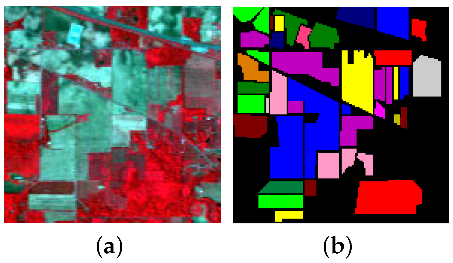
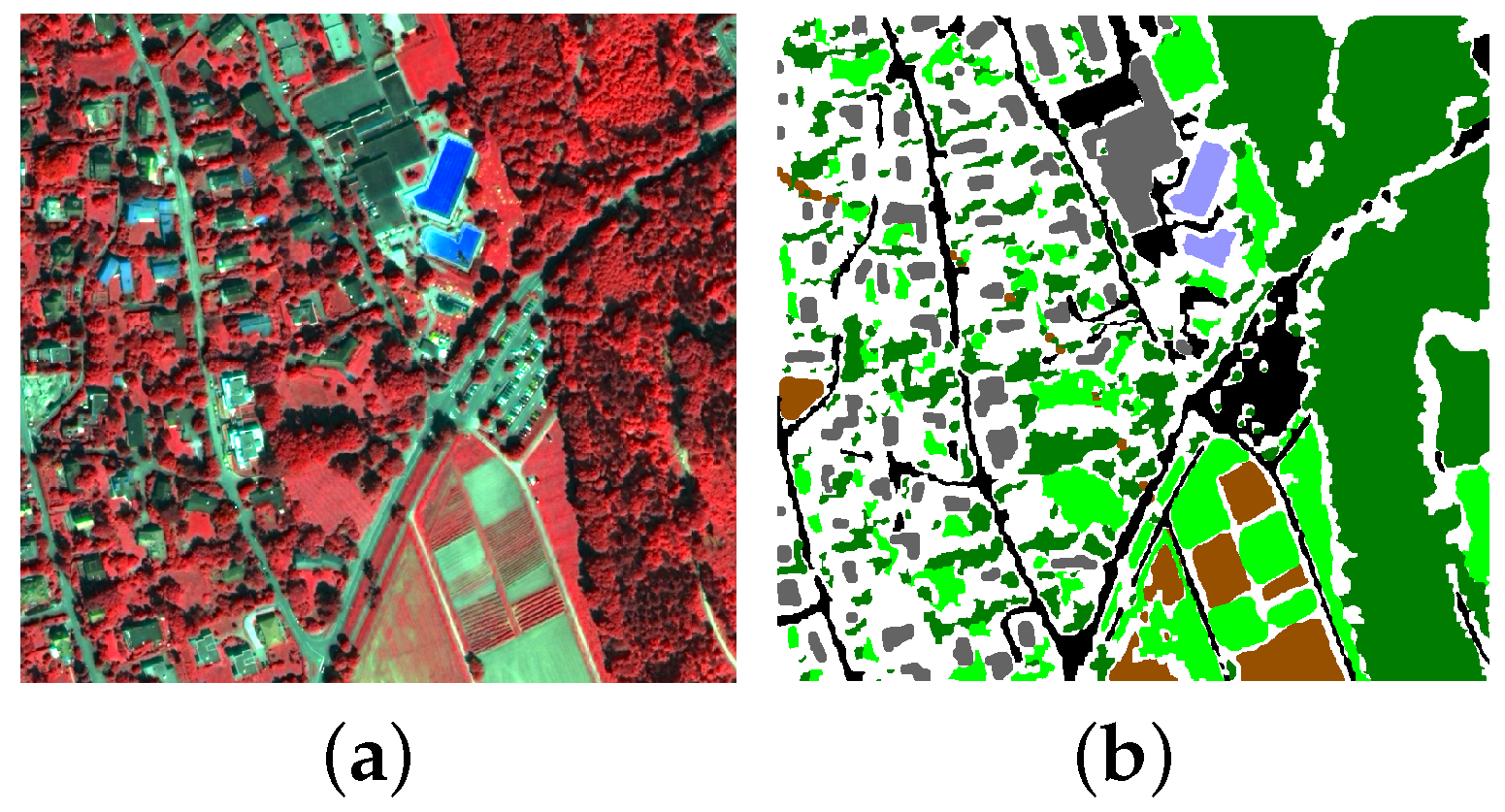
Indian Pines data: the first dataset was gathered by the National Aeronautics and Space Administration’s (NASA) Airborne Visible/Infrared Imaging Spectrometer (AVIRIS) sensor in 1992 over an agricultural area of the Indian Pines test site in northwestern Indiana. The selected scene consists of 145 × 145 pixels and 220 spectral reflectance bands cover the wavelength range of 400 to 2500 nm. After removing 20 bands (i.e., bands 104–108, 150–163 and 220) corrupted by the atmospheric water-vapor absorption effect, 200 bands are considered for experiments. The spatial resolution of this dataset is about 20 m per pixel. The three-band false color composite image together with its corresponding ground truth is depicted in Figure 6. Sixteen different classes of land-covers are considered in the ground truth, which contains 10,366 labeled pixels ranging unbalanced from 20 to 2468, posing a big challenge to the classification problem. The number of training, validation, and testing samples in each class is shown in Table 1, whose background color corresponds to different classes of land-covers. Moreover, note that the total number of samples in class 9 (i.e., Oats) are only 20, and we set the number of validation samples to 5 in this class.
(2)
University of Pavia data: the second dataset was collected by the Reflective Optics System Imaging Spectrometer (ROSIS) over the urban area surrounding the University of Pavia, south of Italy, on 8 July 2002. The dataset contains 103 hyperspectral bands covering the range from 430 to 860 nm and a scene made of 610 × 340 with a spatial resolution of 1.3 m per pixel is considered in the experiment. The three-band false color composite of this data and its corresponding ground truth are shown in Figure 7. We consider nine classes of land-covers in this dataset, and the number of training, validation, and testing samples in each class is shown in Table 2, whose background color distinguishes different classes of land-covers.
(3)
Zurich data: The third dataset was captured by the QuickBird satellite in August 2002 over the city of Zurich, in Switzerland [55]. There are 20 images in the whole dataset and we choose the 18th image for experiments. The chosen image consists of four spectral bands spanning near-infrared to visible spectrum (NIR-R-G-B) and the size of each band is 748 × 800 with a spatial resolution of 0.61 m per pixel. The color composite image and the ground truth are plotted in Figure 8. Six classes of interest are contained in this dataset and the detailed number of training, validation and testing samples in each class is displayed in Table 3, whose background color represents different classes of land-covers.

3.2. Experimental Settings

The purpose of the experiments is to assess the effectiveness of the 3D spatial-adaptive patch construction method and the 3D-SaSiResNet-based classification method. To that end, we utilize the 2D-CNN, 2D-ResNet, 2D Siamese ResNet (abbreviated as 2D-SiResNet), 3D-CNN, 3D-ResNet, and the proposed 3D-SaSiResNet as classifiers, and compare the patches generated in a spatially adaptive fashion with the patches obtained by fixing the training (or validation, testing) samples at the center. Moreover, the SVM [13] by using spectral features is also compared with the 3D-SaSiResNet. As will be shown in Section 3.3, a total of 12 methods are given for comparative study by combining the patch construction and classification methods in pairs. In different methods, the abbreviations containing “Sa” denote spatial-adaptive-based methods, “-fix” denotes 2D or 3D patches are extracted by fixing a certain sample at the center of neighborhood windows, “Si” denotes Siamese-based methods, “−1” denotes a 2D or 3D residual basic block that is used in the ResNet-based methods, “−2” denotes a 2D or 3D ResNeXt basic block that is used in the ResNet-based methods.
The architectures of the above-mentioned deep learning methods are displayed in Table 4, Table 5, Table 6, Table 7, Table 8 and Table 9. It is notable that small kernels are effective choices for 2D-CNN [56] and 3D-CNN [39], and we fix the kernel sizes of all the 2D convolutions to 3 × 3, and most of the 3D convolutions to 3 × 3 × 3. To speed up the 3D-based algorithms and consider more bands at a time, the kernel sizes of the first 3D convolution layers for Indian Pines data, University of Pavia data, and Zurich data are set to 100 × 3 × 3, 50 × 3 × 3 and 3 × 3 × 3, respectively. To make a fair comparison, all the deep learning methods are configured as similar to each other as possible. For instance, the subnetwork in the Siamese-based methods (i.e., 2D-SaSiResNet-1/2D-SaSiResNet-2/2D-SiResNet-2-fix and 3D-SaSiResNet-1/3D-SaSiResNet-2/3D-SiResNet-2-fix) are set up identical to the corresponding non-Siamese ones (i.e., 2D-SaCNN/2D-SaResNet-1/2D-SaResNet-2 and 3D-SaCNN/3D-SaResNet-1/3D-SaResNet-2), and the number of layers in the 2D-based networks are the same as the 3D-based ones. For the parameter settings, the intrinsic dimensionalities are calculated to be 5, 4, and 2 in the Indian Pines data, University of Pavia data, and Zurich data, respectively, and the number of superpixels are set to 589, 2602, and 19,543 in the three multiband images datasets, respectively. The patch size w of all the three experimental datasets is set to 9. In other words, each sample is represented by its 9 × 9 neighborhoods in 2D-SiResNet-2-fix and 3D-SiResNet-2-fix, while all the spatial-adaptive patches are resized to 9 × 9 so as to represent the objects of the multiband images. The reasons for resizing the patches to 9 × 9 are that, if w is too small (e.g., 3 × 3), the spatial information will not be adequately learned by the network; on the contrary, if w is too large (e.g., 15 × 15), the computational burden will be increased and the training process will slow down. The batch size and training epochs are taken as 20 and 100, respectively. Furthermore, the Adam solver is adopted to train the networks and the learning rate is initialized to 0.0001.
Moreover, the SVM and 3D spatial-adaptive patches generation procedure is performed by MATLAB R2019a (The MathWorks, United States) on a Windows 10 operating system (Microsoft, United States) and the deep learning-based classification methods are executed on a server with Nvidia Tesla K80 GPU platform (NVIDIA, United States) and Pytorch backend. In all three datasets, very limited labeled samples, i.e., 10 samples per class, are randomly chosen as training samples, 10 (or 5 samples in class 9 (i.e., Oats) of the Indian Pines data) per class are for validation and the rest are for testing. To study the influence of the number of training samples, we also choose 20 and 50 samples from each class for training. Since classes 1 (i.e., Alfalfa), 7 (i.e., Grass/pasture-mowed), and 9 (i.e., Oats) contain very few samples for the Indian Pines data, the number of training samples in those classes is constantly set to 10 in different cases. The number of validation samples is the same as that in Table 1, Table 2 and Table 3. The label of a training patch is set to be the same as that of most training samples in this patch. In case the training patches of a certain class are less than 2, we perform rotation augmentation, whose rotation angle is 90 degrees, to augment the number of training patches to 2. Three popular indices, i.e., overall accuracy (OA), average accuracy (AA), and kappa coefficient ( κ ), are computed to compare different methods quantitatively. All three of the indices are obtained by comparing the reference labels and the calculated labels of test samples. Each experiment is repeated ten times using a repeated random subsampling validation strategy to alleviate possible bias and the average results are displayed in the tables.

3.3. Classification Results

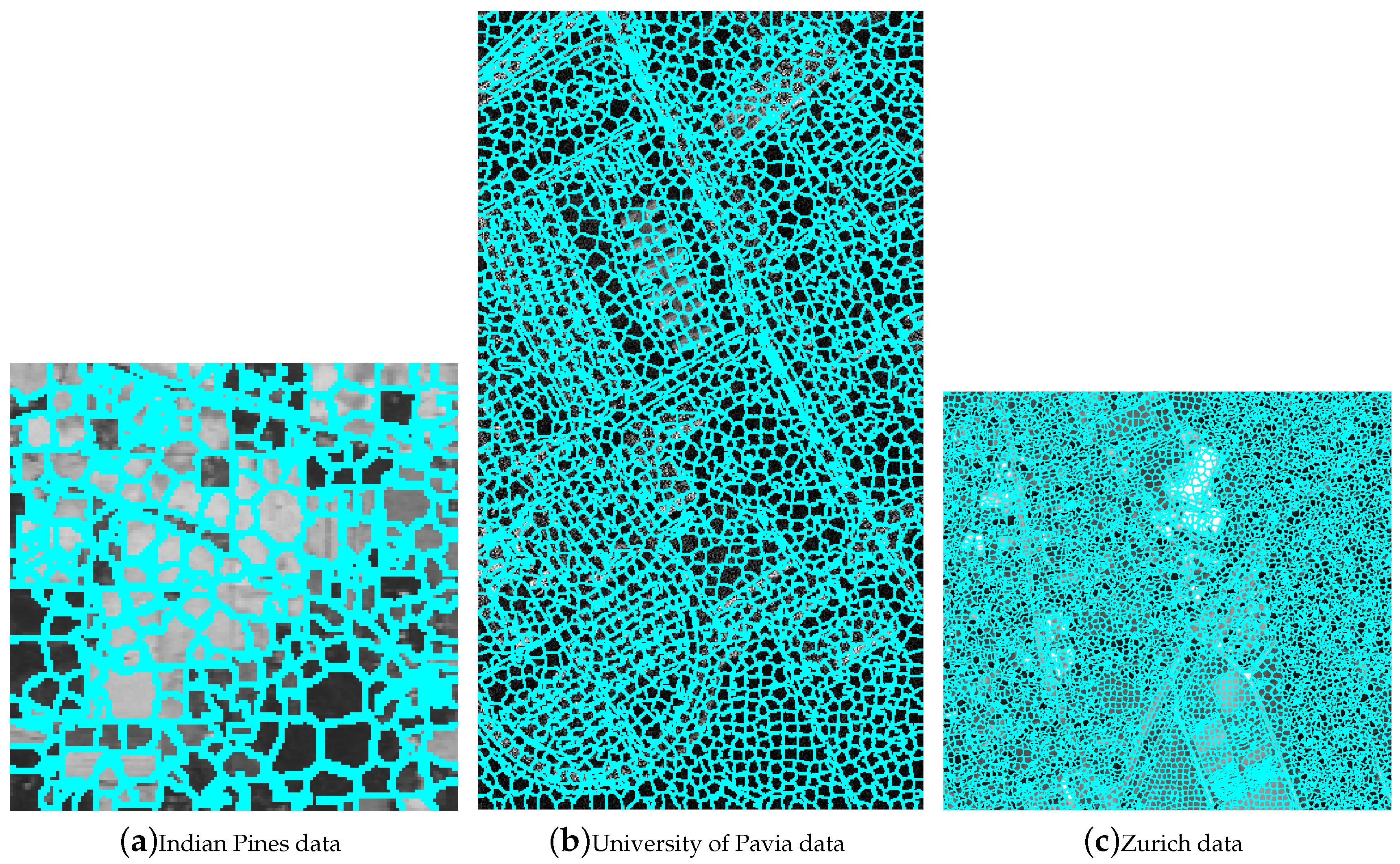
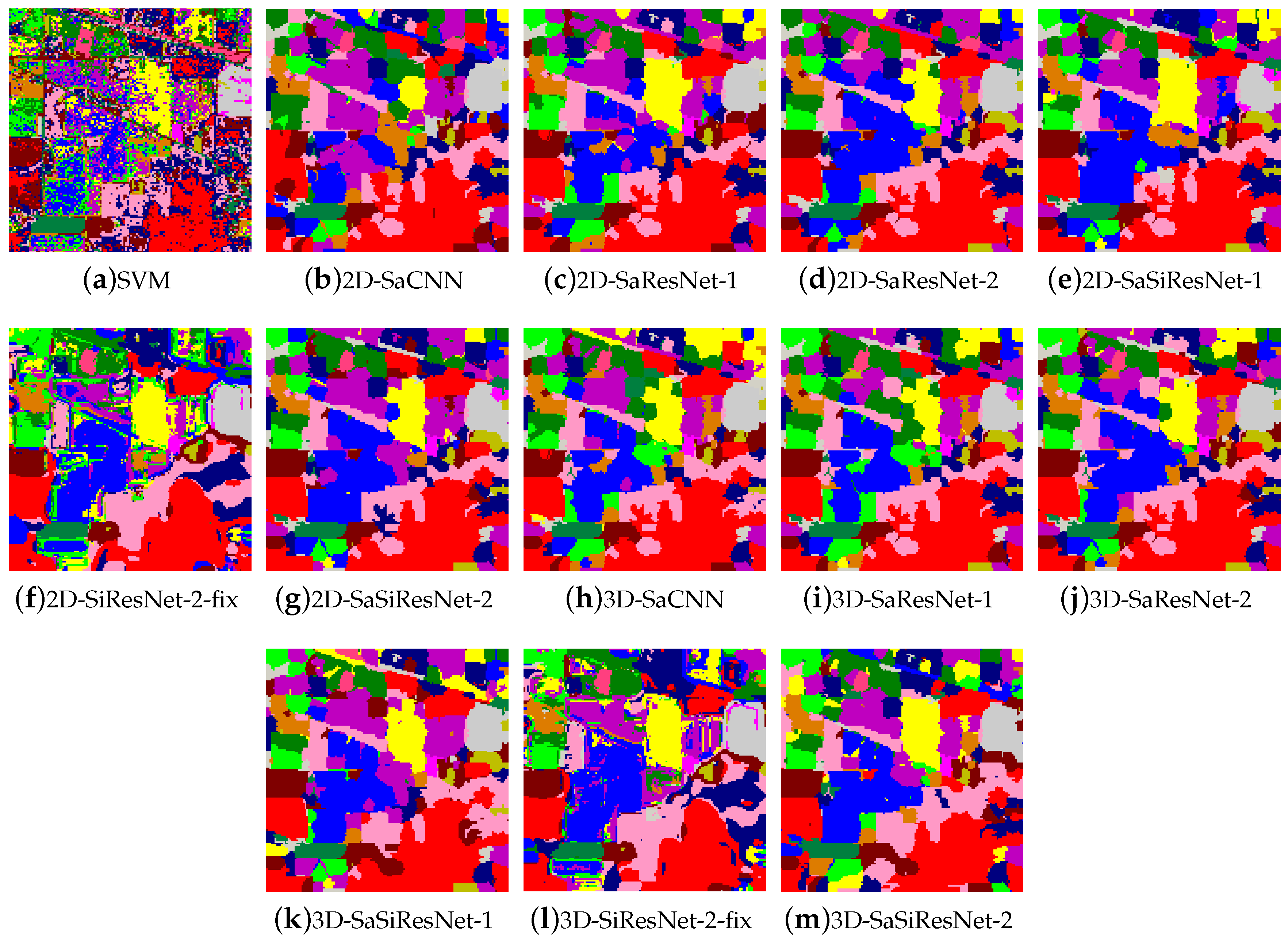
The final superpixel segmentation results of the three experimental datasets are shown in Figure 9, from which we find that the proposed superpixel map generation method flexibly divides the multiband images data into naturally formed spatial areas with irregular sizes and shapes. Table 10, Table 11 and Table 12 report the class-specific accuracy, OA, AA, κ , and computation time of different methods, while the thematic maps are visually depicted in Figure 10, Figure 11 and Figure 12. According to the reported results, a few observations are noteworthy. It can be first seen that, in most cases, the spatial-adaptive patches outperforms the patches generated by fixing the training/validation/testing samples at the center. As an example, for the Indian Pines data, the OA and κ of the 2D-SaSiResNet-2 are respectively 8.24% and 9.00% higher than the 2D-SiResNet-2-fix (see Table 10), while the improvement in OA of the 3D-SaSiResNet-2 is at least 3% more than its corresponding fixed center version (i.e., 3D-SiResNet-2-fix). We can observe from Figure 10 that the classification maps of 2D-SaSiResNet-2/3D-SaSiResNet-2 are much less noisy than those of the 2D-SiResNet-2-fix/3D-SiResNet-2-fix. For the University of Pavia data (see Table 11) and Zurich data (see Table 12), although the improvement in classification accuracy is not as much as the Indian Pines data, the methods with spatial-adaptive patches still provide better results than those with a fixed center in most situations. It is shown in Figure 11 that 2D-SiResNet-2-fix/3D-SiResNet-2-fix fail to correctly classify the pixels in some regions (e.g., the Bricks (class 8) located at the middle-left region), while 2D-SaSiResNet-2/3D-SaSiResNet-2 give a better classification performance than 2D-SiResNet-2-fix/3D-SiResNet-2-fix. Moreover, as shown in Figure 12, the classification maps of 2D-SiResNet-2-fix/3D-SiResNet-2-fix assign more areas to Road (class 1). This makes the classification accuracy of the Road (class 1) higher than 2D-SaSiResNet-2/3D-SaSiResNet-2; nevertheless, it sacrifices the accuracy of other land-covers. The reason for good results of the spatial-adaptive patch construction method is that they can take into consideration the spatial structures and region boundary areas of the remote sensing data while its counterpart forcibly divides the data into fixed center patches, ignoring the heterogeneous land covers, especially those at the border of different classes.
We then compare the 3D-SaSiResNet-1/3D-SaSiResNet-2 against other methods. It can be observed from Table 10, Table 11 and Table 12 that SVM and 2D-SaCNN perform the worst, the 3D-SaCNN, 2D-SaResNet-1/2D-SaResNet-2, and 3D-SaResNet-1/3D-SaResNet-2 have better performances than the SVM and 2D-SaCNN but comparable or slightly inferior to the 2D-SaSiResNet-1/2D-SaSiResNet-2, and 3D-SaSiResNet-1/3D-SaSiResNet-2 yield superior performance to the competing methods. As given in Table 10, the OA of the SVM and 2D-SaCNN are at least 10% lower than the 3D-SaCNN, 2D-SaResNet-1/2D-SaResNet-2 and 3D-SaResNet-1/3D-SaResNet-2 for the Indian Pines data. It can be obviously seen from Table 11 and Table 12 that the classification performance of the SVM and 2D-SaCNN is also worse than the 3D-SaCNN, 2D-SaResNet-1/2D-SaResNet-2, and 3D-SaResNet-1/3D-SaResNet-2 for the other two datasets. One reason why 3D-SaCNN performs better than SVM and 2D-SaCNN is that the 3D convolution can simultaneously extract the spectral-spatial features, and the reason why 2D-SaResNet-1/2D-SaResNet-2 outperform 2D-SaCNN is mainly because shortcut connections are adopted to improve the effectiveness of the training procedure. Moreover, the Siamese-based methods perform much better than their corresponding no-Siamese versions. Specifically, it is notable from Table 10 that the 3D-SiSaResNet-2 provides the best performance in all the algorithms under comparison. Classification results of the University of Pavia data and Zurich data also reveal similar properties. This implies that the Siamese architecture of the network combined with 3D ResNet can effectively improve the classification performance. The main reason why the Siamese architecture is suitable for classification of multiband images with very few training samples is because the network is trained by inputting the training samples in pairs and thus the separability of different classes are learned and the features extracted are especially suitable for the classification task.
An additional noticeable point is that the 3D-based classification methods achieve comparable or better performance than the 2D-based ones. As illustrated in Table 11, in comparison with the 2D-SaCNN, the OA of 3D-SaCNN is improved by 8.79% for the University of Pavia, while the OA of 3D-SaSiResNet-2 is 2.84% higher than its 2D scenario (i.e., 2D-SaSiResNet-2). Similarly, it can be found from Table 10, Table 11 and Table 12 that the 3D-SaCNN, 3D-SaResNet-1/3D-SaResNet-2, 3D-SaSiResNet-1/3D-SaSiResNet-2, and 3D-SiResNet-2-fix have better classification results than their corresponding 2D versions. Moreover, it is also clearly visible from Figure 10, Figure 11 and Figure 12 that the classification maps of the 3D-based methods are much closer to the ground truth (see Figure 6b, Figure 7b and Figure 8b) than the 2D-based ones. This is due to the fact that, by representing the multiband images in 3D cubes, the joint spectral-spatial structures are effectively learned by the 3D-based classification methods.
To further validate the effectiveness of the proposed method, we focus on the features learned by the last layer of various deep learning-based methods. It is notable from Table 10 that the land covers Corn-no till (class 2), Corn-min till (class 3), and Soybean-no till (class 10) are difficult-to-separate classes for the Indian Pines data. For instance, as for class 3, the classification accuracy of the 2D-SaCNN is as low as 43.21%, the 2D-SaSiResNet-2 and 3D-SaSiResNet-2 significantly improve the classification performance, and the classification accuracy of the 3D-SaSiResNet-2 is increased to 81.92%. As for class 2 and class 10, the proposed 3D-SaSiResNet-2 also provides better results than the state-of-the-art methods. To give an intuitive explanation, the two-dimensional features of the Indian Pines data obtained by 2D-SaCNN, 2D-SaSiResNet-2, 3D-SiResNet-2-fix, and 3D-SaSiResNet-2 in a trial are plotted in Figure 13, from which we can see that the representations learned by the 3D-SaSiResNet-2 are more scattered and separable than other methods. Therefore, it is much easier to distinguish the samples with the features obtained by the 3D-SaSiResNet-2. Moreover, as can be observed from Table 10, Table 11 and Table 12, although 3D-SaSiResNet-1 and 3D-SaSiResNet-2 take more computation time than no-Siamese-based methods, they are much more efficient than the 2D-SiResNet-2-fix and 3D-SiResNet-2-fix for the Indian Pines data and Zurich data. As to the University of Pavia data, although the processing time of 3D-SaSiResNet-1/3D-SaSiResNet-2 is about four minutes longer than 2D-SiResNet-2-fix/3D-SiResNet-2-fix, they can complete the classification task in less than 20 min. 3D-SaSiResNet-1/3D-SaSiResNet-2 are efficient because they are object-based methods rather than pixel-based methods, and the kernel sizes of the first 3D convolution layers are set to 100 × 3 × 3 and 50 × 3 × 3 in the two hyperspectral datasets rather than 3 × 3 × 3. In short, the experimental results validate the effectiveness of 3D-SaSiResNet in the classification of multiband images data.

3.4. Parameter Analysis

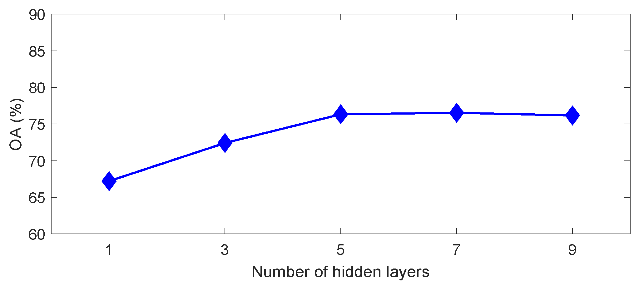
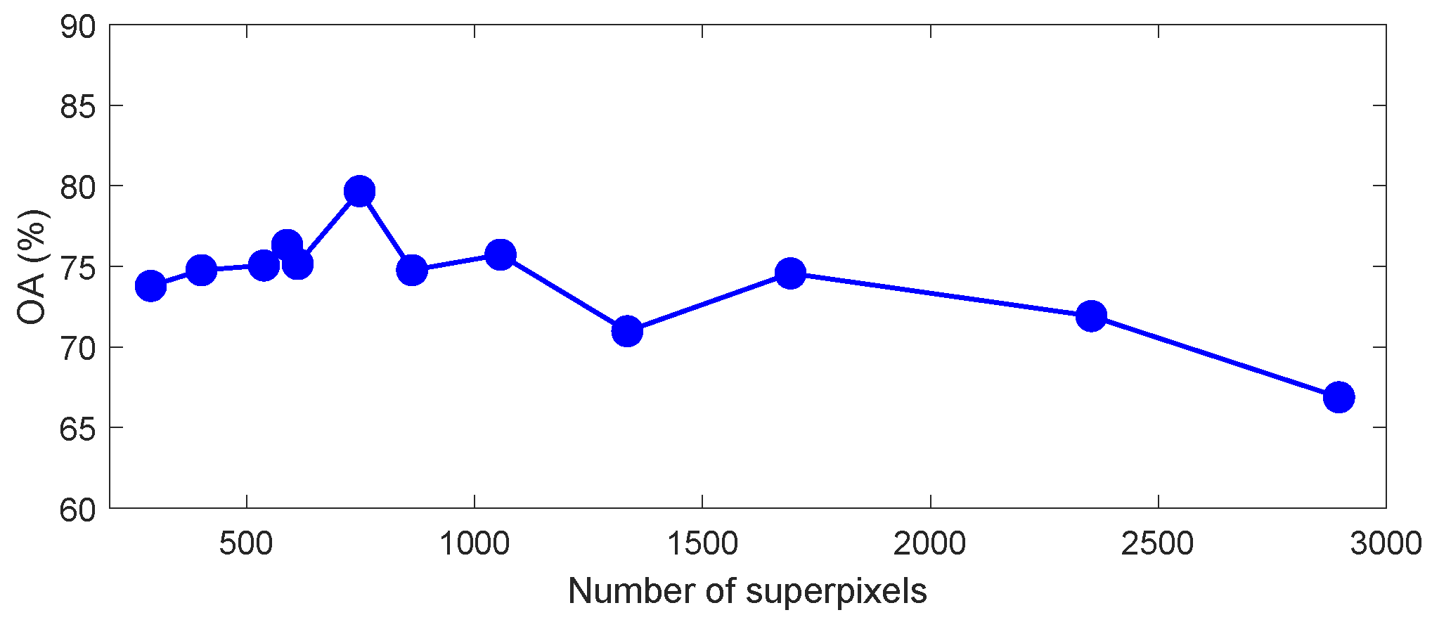
In this section, the influence of four important parameters, i.e., the number of hidden layers in SAE for band reduction of the hyperspectral image, the number of training samples, the number of superpixels, and the number of training epochs on the performance of the proposed method, is discussed. Figure 14, Figure 15, Figure 16 and Figure 17 show the OA of the proposed method when the four parameters vary.
As shown in Figure 14, we set the number of hidden layers in SAE as 1 (the number of the unit is set to 5), 3 (the number of units is set to 100, 25 and 5, respectively), 5 (the number of units is set to 100, 50, 25, 10 and 5, respectively), 7 (the number of units is set to 150, 100, 75, 50, 25, 10, and 5, respectively), and 9 (the number of units is set to 175, 150, 125, 100, 75, 50, 25, 10, and 5, respectively), and the classification accuracy varies with the different number of hidden layers. It can be observed that the OA is relatively low when the number of hidden layers is 1 or 3. When the number of hidden layers is equal to or larger than 5, the classification performance is satisfactory. In this paper, we set the number of hidden layers to 5 since more hidden layers will increase the complexity of the model.
Figure 15 depicts the OA of different methods with various numbers of training samples for the Indian Pines data. The number of training samples in classes 1, 7, and 9 is constantly set to 10 in different cases. It can be seen from Figure 15 that the classification performance of all considered methods yields stable improvement with the increase of the training set size. For instance, the OA of 2D-SaCNN is lower than 60% in case 10 training samples per class are selected and is increased to more than 70% with 50 training samples per class. This stresses again the importance of training samples for multiband images classification. Moreover, it can be concluded from Figure 15 that the 3D-SaSiResNet has better classification performance than the Siamese convolutional neural network (S-CNN) proposed in [45]. This is because, when the number of training samples in each class equals 50, the classification accuracy of S-CNN is lower than 90% (see Figure 20 in [45]), while the accuracy of our proposed method is higher than 90% with 16 rather than nine classes of land-covers and using 50 training samples per class.
Figure 16 plots the OA against the number of superpixels for the Indian Pines data. The number of superpixels is varied within the range from 290 to 2896. We can observe that a dramatically upward tendency appeared with an initial increase of superpixel number, and the classification accuracy decreases in case the number of superpixels is over a certain value (e.g., 1057). Based on the above analysis, too small and too large number of superpixels may be harmful to the classification performance, and it is better to utilize suitable superpixel numbers according to the object characteristics’ spatial structure of the remote sensing data.
Furthermore, the impact of the number of training epochs is depicted in Figure 17. It can be seen that the OA rapidly increases in the first couple of epochs and then improves slowly as the number of epochs increases. Finally, the OA trends to a certain stable value with the increased number of epochs. As shown in Figure 17, it is suggested that the 3D-SaSiResNet-2 is trained more than 30 epochs to obtain stable and effective classification performance.

3.5. Discussion

In this paper, the three datasets are benchmark and widely-used in remote sensing classification. In the experiments, the Indian Pines data gain more improvement in classification accuracy than the other two datasets. The reason why Indian Pines data achieve more discriminative results than the other two datasets is that the spatial resolution of Indian Pines data (i.e., 20 m) is much lower than that of the Pavia (i.e., 1.3 m) and Zurich datasets (i.e., 0.61 m). Therefore, in the Indian Pines data, the region represented by the same number of pixels may contain more different types of land-covers than the other two datasets. It is noteworthy that the proposed 3D-SaSiResNet can better distinguish the boundaries of different land-covers, and our spatial-adaptive-based method has a higher advantage in the classification of Indian Pines data. We perform statistical significance analysis to further confirm the effectiveness of the proposed method. The statistical difference between the proposed 3D-SaSiResNet-2 and competing methods is studied by the McNemar’s test, which is achieved by the standardized normal test statistic
Z = f 12 f 21 f 12 + f 21 ,
where f i j , ( i , j = 1 , 2 ) denotes the number of samples correctly classified by the classifier i but incorrectly classified by the classifier j and Z is the pairwise statistical significance of the difference between the ith and jth classifiers. If | Z | > 1 . 96 , the classification difference of the two classifiers is considered as statistically significant at the 5% level of significance. It is shown in Table 13 that the 3D-SaSiResNet-2 is statistically superior ( | Z | > 1 . 96 ) to all of the other methods except the 3D-SaSiResNet-1 ( | Z | < 1 . 96 ) for the Indian Pines data. Moreover, Figure 13 intuitively compares the separability of the features learned by different methods according to choosing three difficult-to-separate classes for the Indian Pines data. It is observed that the features obtained by the proposed method are easier to distinguish than other methods.
In the 3D-SaSiResNet, the nearest neighbor classifier is used to classify the learned features of testing samples. The nearest neighbor classifier can be replaced by other sophisticated classifies (e.g., k-nearest neighbor (KNN), SVM or Softmax layer), and it can be treated as a special case of KNN with k = 1 . It is worth noting that, in case the training set is quite small, the nearest neighbor classifier provides better classification performance than other sophisticated classifiers, while KNN, SVM, or the Softmax layer has higher accuracy than the nearest neighbor classifier if more training samples are available.
The classification results shown in Table 10, Table 11 and Table 12 seems a little bit low. For instance, the highest OA in Table 10 is lower than 80%. In addition, there is a lagging between OA and κ . The reason for the above phenomena is that we only choose a small training set (i.e., training samples per class are no more than 10) in the experiment. The number of training samples is essential to the classification accuracies of various methods. The classification performance of a certain method with a small training set is more likely inferior to the situation with a big training set. As shown in Figure 15, the OA of 3D-SaSiResNet-2 is higher than 90% with 50 training samples per class (except the classes 1, 7, and 9). Moreover, the gap between OA and Kappa will decrease with the increase of training samples.

4. Conclusions

In this paper, we have proposed a deep network architecture, namely 3D-SaSiResNet, for classification of the multiband images data. The underlying idea of 3D-SaSiResNet is to explore the spatial-adaptive and discriminative features that make the samples from the same class close and those belonging to different classes separated. Based on this concept, 3D spatial-adaptive patches are constructed by superpixel segmentation. In contrast to previous approaches that fix the samples at the center, the patches generated by superpixels do not force the samples at the center but flexibly make the neighbors within the same patch be more likely to come from the same class. Moreover, the network has a Siamese architecture composed of two 3D-ResNet-based subnetworks, which are pairwise trained to increase the separability of different classes. The unlabeled testing samples can be fed into the trained network and classified by a simple nearest neighbor classifier. Experiments on three multiband images datasets acquired by different sensors have demonstrated that the proposed 3D-SaSiResNet method outperforms the state-of-the-art techniques in terms of visual quality and recognition performance. Comparisons show that the 3D-SaSiResNet is especially effective in case limited samples are available for training. The main disadvantage of 3D-SaSiResNet is that the running time of the 3D spatial adaptive patch construction step is much longer than that of the 2D-SiResNet-2-fix and 3D-SiResNet-2-fix. In future works, we will try to adaptively determine the optimal number of superpixels for different datasets and improve the proposed method by deformable convolutions. Classifying unbalanced samples, especially the number of samples in some categories that are particularly small, is one of our future activities. Moreover, it would be a great interest to improve the computational efficiency of the Siamese architecture by pruning and quantization.

Author Contributions

All coauthors made significant contributions to the manuscript. Z.H. designed the research framework, analyzed the results, and wrote the manuscript. D.H. assisted in the prepared work and validation work. Moreover, all coauthors contributed to the editing and review of the manuscript. All authors have read and agreed to the published version of the manuscript.

Funding

This research was funded by the National Key R&D Program of China, grant numbers 2018YFB0505500 and 2018YFB0505503; the Guangdong Basic and Applied Basic Research Foundation, grant number 2019A1515011877; the Guangzhou Science and Technology Planning Project, grant number 202002030240; the Fundamental Research Funds for the Central Universities, grant number 19lgzd10; the National Natural Science Foundation of China, grant numbers 41501368 and 4153117; the Southern Marine Science and Engineering Guangdong Laboratory (Zhuhai), grant number 99147-42080011; the 2018 Key Research Platforms and Research Projects of Ordinary Universities in GuangDong Province, grant number 2018KQNCX360.

Acknowledgments

The authors would like to take this opportunity to thank the Editors and the Anonymous Reviewers for their detailed comments and suggestions, which greatly helped us to improve the clarity and presentation of our manuscript.

Conflicts of Interest

The authors declare no conflict of interest.

References

  1. Sun, W.; Jiang, M.; Li, W.; Liu, Y. A symmetric sparse representation based band selection method for hyperspectral imagery classification. Remote Sens. 2016, 8, 238. [Google Scholar] [CrossRef] [Green Version]
  2. Li, J.; Liu, Z. Multispectral transforms using convolution neural networks for remote sensing multispectral image compression. Remote Sens. 2019, 11, 759. [Google Scholar] [CrossRef] [Green Version]
  3. Feng, J.; Feng, X.; Chen, J.; Cao, X.; Zhang, X.; Jiao, L.; Yu, T. Generative adversarial networks based on collaborative learning and attention mechanism for hyperspectral image classification. Remote Sens. 2020, 12, 1149. [Google Scholar] [CrossRef] [Green Version]
  4. Nezami, S.; Khoramshahi, E.; Nevalainen, O.; Pölönen, I.; Honkavaara, E. Tree species classification of drone hyperspectral and rgb imagery with deep learning convolutional neural networks. Remote Sens. 2020, 12, 1070. [Google Scholar] [CrossRef] [Green Version]
  5. Padró, J.C.; Muñoz, F.J.; Planas, J.; Pons, X. Comparison of four UAV georeferencing methods for environmental monitoring purposes focusing on the combined use with airborne and satellite remote sensing platforms. Int. J. Appl. Earth Obs. Geoinf. 2019, 75, 130–140. [Google Scholar] [CrossRef]
  6. Zheng, Z.; Du, S.; Wang, Y.C.; Wang, Q. Mining the regularity of landscape-structure heterogeneity to improve urban land-cover mapping. Remote Sens. Environ. 2018, 214, 14–32. [Google Scholar] [CrossRef]
  7. Olteanu-Raimond, A.M.; See, L.; Schultz, M.; Foody, G.; Riffler, M.; Gasber, T.; Jolivet, L.; le Bris, A.; Meneroux, Y.; Liu, L.; et al. Use of automated change detection and vgi sources for identifying and validating urban land use change. Remote Sens. 2020, 12, 1186. [Google Scholar] [CrossRef] [Green Version]
  8. Yao, X.; Zhao, C. Hyperspectral anomaly detection based on the bilateral filter. Infrared Phys. Technol. 2018, 92, 144–153. [Google Scholar] [CrossRef]
  9. Fauvel, M.; Tarabalka, Y.; Benediktsson, J.A.; Chanussot, J.; Tilton, J.C. Advances in spectral-spatial classification of hyperspectral images. Proc. IEEE 2013, 101, 652–675. [Google Scholar] [CrossRef] [Green Version]
  10. Lu, X.; Zheng, X.; Yuan, Y. Remote sensing scene classification by unsupervised representation learning. IEEE Trans. Geosci. Remote Sens. 2017, 55, 5148–5157. [Google Scholar] [CrossRef]
  11. Li, Z.; Tang, X.; Li, W.; Wang, C.; Liu, C.; He, J. A two-stage deep domain adaptation method for hyperspectral image classification. Remote Sens. 2020, 12, 1054. [Google Scholar] [CrossRef] [Green Version]
  12. Cortes, C.; Vapnik, V. Support-vector networks. Machine learning 1995, 20, 273–297. [Google Scholar] [CrossRef]
  13. Chang, C.C.; Lin, C.J. LIBSVM: A library for support vector machines. ACM Trans. Intell. Syst. Technol. 2011, 2, 27:1–27:27. Available online: http://www.csie.ntu.edu.tw/~cjlin/libsvm (accessed on 2 May 2020). [CrossRef]
  14. Paoletti, M.E.; Haut, J.M.; Tao, X.; Miguel, J.P.; Plaza, A. A new GPU implementation of support vector machines for fast hyperspectral image classification. Remote Sens. 2020, 12, 1257. [Google Scholar] [CrossRef] [Green Version]
  15. Benediktsson, J.A.; Palmason, J.A.; Sveinsson, J.R. Classification of hyperspectral data from urban areas based on extended morphological profiles. IEEE Trans. Geosci. Remote Sens. 2005, 43, 480–491. [Google Scholar] [CrossRef]
  16. Mura, M.D.; Villa, A.; Benediktsson, J.A.; Chanussot, J.; Bruzzone, L. Classification of Hyperspectral Images by Using Extended Morphological Attribute Profiles and Independent Component Analysis. IEEE Geosci. Remote Sens. Lett. 2011, 8, 542–546. [Google Scholar] [CrossRef] [Green Version]
  17. Tsai, F.; Lai, J.S. Feature extraction of hyperspectral image cubes using three-dimensional gray-level cooccurrence. IEEE Trans. Geosci. Remote Sens. 2013, 51, 3504–3513. [Google Scholar] [CrossRef]
  18. Jia, S.; Shen, L.; Li, Q. Gabor feature-based collaborative representation for hyperspectral imagery classification. IEEE Trans. Geosci. Remote Sens. 2015, 53, 1118–1129. [Google Scholar] [CrossRef]
  19. Yin, J.; Gao, C.; Jia, X. Wavelet Packet Analysis and Gray Model for Feature Extraction of Hyperspectral Data. IEEE Geosci. Remote Sens. Lett. 2013, 10, 682–686. [Google Scholar] [CrossRef]
  20. Achanta, R.; Shaji, A.; Smith, K.; Lucchi, A.; Fua, P.; Süsstrunk, S. SLIC superpixels compared to state-of-the-art superpixel methods. IEEE Trans. Pattern Anal. Mach. Intell. 2012, 34, 2274–2282. [Google Scholar] [CrossRef] [Green Version]
  21. Liu, T.; Gu, Y.; Chanussot, J.; Mura, M.D. Multimorphological Superpixel Model for Hyperspectral Image Classification. IEEE Trans. Geosci. Remote Sens. 2017, 55, 6950–6963. [Google Scholar] [CrossRef]
  22. Zhang, H.; Li, J.; Huang, Y.; Zhang, L. A nonlocal weighted joint sparse representation classification method for hyperspectral imagery. IEEE J. Sel. Top. Appl. Earth Obs. Remote Sens. 2014, 7, 2056–2065. [Google Scholar] [CrossRef]
  23. He, Z.; Wang, Q.; Shen, Y.; Sun, M. Kernel sparse multitask learning for hyperspectral image classification with empirical mode decomposition and morphological wavelet-based features. IEEE Trans. Geosci. Remote Sens. 2014, 52, 5150–5163. [Google Scholar] [CrossRef]
  24. Tarabalka, Y.; Fauvel, M.; Chanussot, J.; Benediktsson, J.A. SVM- and MRF-based method for accurate classification of hyperspectral images. IEEE Geosci. Remote Sens. Lett. 2010, 7, 736–740. [Google Scholar] [CrossRef] [Green Version]
  25. Zhang, L.; Zhang, L.; Tao, D.; Huang, X. Tensor discriminative locality alignment for hyperspectral image spectral-spatial feature extraction. IEEE Trans. Geosci. Remote Sens. 2013, 51, 242–256. [Google Scholar] [CrossRef]
  26. He, Z.; Li, J.; Liu, L. Tensor block-sparsity based representation for spectral-spatial hyperspectral image classification. Remote Sens. 2016, 8, 636. [Google Scholar] [CrossRef] [Green Version]
  27. Zhong, Z.; Fan, B.; Duan, J.; Wang, L.; Ding, K.; Xiang, S.; Pan, C. Discriminant tensor spectral-spatial feature extraction for hyperspectral image classification. IEEE Geosci. Remote Sens. Lett. 2015, 12, 1028–1032. [Google Scholar] [CrossRef]
  28. Zhang, L.; Zhang, L.; Du, B. Deep learning for remote sensing data: A technical tutorial on the state of the art. IEEE Geosci. Remote Sens. Mag. 2016, 4, 22–40. [Google Scholar] [CrossRef]
  29. Li, S.; Song, W.; Fang, L.; Chen, Y.; Ghamisi, P.; Benediktsson, J.A. Deep learning for hyperspectral image classification: An overview. IEEE Trans. Geosci. Remote Sens. 2019, 57, 6690–6709. [Google Scholar] [CrossRef] [Green Version]
  30. Wang, S.; Quan, D.; Liang, X.; Ning, M.; Guo, Y.; Jiao, L. A deep learning framework for remote sensing image registration. ISPRS J. Photogramm. Remote Sens. 2018, 145, 148–164. [Google Scholar] [CrossRef]
  31. Dong, G.; Liao, G.; Liu, H.; Kuang, G. A review of the autoencoder and its variants: A comparative perspective from target recognition in synthetic-aperture radar images. IEEE Geosci. Remote Sens. Mag. 2018, 6, 44–68. [Google Scholar] [CrossRef]
  32. Chen, Y.; Lin, Z.; Zhao, X.; Wang, G.; Gu, Y. Deep learning-based classification of hyperspectral data. IEEE J. Sel. Top. Appl. Earth Obs. Remote Sens. 2014, 7, 2094–2107. [Google Scholar] [CrossRef]
  33. Chen, Y.; Zhao, X.; Jia, X. Spectral-spatial classification of hyperspectral data based on deep belief network. IEEE J. Sel. Topics Appl. Earth Obs. Remote Sens. 2015, 8, 2381–2392. [Google Scholar] [CrossRef]
  34. He, K.; Zhang, X.; Ren, S.; Sun, J. Deep residual learning for image recognition. In Proceedings of the IEEE Conference on Computer Vision and Pattern Recognition, Las Vegas, NV, USA, 26 June–1 July 2016; pp. 770–778. [Google Scholar]
  35. He, Z.; Liu, H.; Wang, Y.; Hu, J. Generative adversarial networks-based semi-supervised learning for hyperspectral image classification. Remote Sens. 2017, 9, 1042. [Google Scholar] [CrossRef] [Green Version]
  36. Hu, W.; Huang, Y.; Wei, L.; Zhang, F.; Li, H. Deep convolutional neural networks for hyperspectral image classification. J. Sens. 2015, 2015, 1–12. [Google Scholar] [CrossRef] [Green Version]
  37. Yue, J.; Zhao, W.; Mao, S.; Liu, H. Spectral-spatial classification of hyperspectral images using deep convolutional neural networks. Remote Sens. Lett. 2015, 6, 468–477. [Google Scholar] [CrossRef]
  38. Cheng, G.; Yang, C.; Yao, X.; Guo, L.; Han, J. When deep learning meets metric learning: Remote sensing image scene classification via learning discriminative CNNs. IEEE Trans. Geosci. Remote Sens. 2018, 56, 2811–2821. [Google Scholar] [CrossRef]
  39. Li, Y.; Zhang, H.; Shen, Q. Spectral-spatial classification of hyperspectral imagery with 3D convolutional neural network. Remote Sens. 2017, 9, 67. [Google Scholar] [CrossRef] [Green Version]
  40. Hamida, A.B.; Benoit, A.; Lambert, P.; Amar, C.B. 3-D deep learning approach for remote sensing image classification. IEEE Trans. Geosci. Remote Sens. 2018, 56, 4420–4434. [Google Scholar] [CrossRef] [Green Version]
  41. Zhong, Z.; Li, J.; Luo, Z.; Chapman, M. Spectral-spatial residual network for hyperspectral image classification: A 3-D deep learning framework. IEEE Trans. Geosci. Remote Sens. 2018, 56, 847–858. [Google Scholar] [CrossRef]
  42. Koch Gregory, R.Z.; Salakhutdinov, R. Siamese neural networks for one-shot image recognition. In Proceedings of the ICML Deep Learning Workshop, Lille, France, 6–11 July 2015; Volume 2. [Google Scholar]
  43. Liu, B.; Yu, X.; Yu, A.; Zhang, P.; Wan, G.; Wang, R. Deep Few-Shot Learning for Hyperspectral Image Classification. IEEE Trans. Geosci. Remote Sens. 2018, 57, 2290–2304. [Google Scholar] [CrossRef]
  44. Liu, B.; Yu, X.; Yu, A.; Wan, G. Deep convolutional recurrent neural network with transfer learning for hyperspectral image classification. J. Appl. Remote Sens. 2018, 12, 026028. [Google Scholar] [CrossRef]
  45. Liu, B.; Yu, X.; Zhang, P.; Yu, A.; Fu, Q.; Wei, X. Supervised deep feature extraction for hyperspectral image classification. IEEE Trans. Geosci. Remote Sens. 2017, 56, 1909–1921. [Google Scholar] [CrossRef]
  46. Zhao, S.; Li, W.; Du, Q.; Ran, Q. Hyperspectral classification based on siamese neural network using spectral-spatial feature. In Proceedings of the IGARSS 2018-2018 IEEE International Geoscience and Remote Sensing Symposium, Valencia, Spain, 22–27 July 2018; pp. 2567–2570. [Google Scholar]
  47. Hinton, G.E.; Zemel, R.S. Autoencoders, minimum description length and helmholtz free energy. In Advances in Neural Information Processing Systems 6; Cowan, J.D., Tesauro, G., Alspector, J., Eds.; Morgan-Kaufmann: Burlington, MA, USA, 1994; pp. 3–10. [Google Scholar]
  48. Bengio, Y.; Lamblin, P.; Popovici, D.; Larochelle, H. Greedy layer-wise training of deep networks. In Proceedings of the 19th International Conference on Neural Information Processing Systems; Doha, Qatar, 12–15 November 2006, MIT Press: Cambridge, MA, USA, 2006; pp. 153–160. [Google Scholar]
  49. Van Der Maaten, L.; Postma, E.; Van den Herik, J. Dimensionality reduction: A comparative review. J. Mach. Learn. Res. 2009, 10, 66–71. [Google Scholar]
  50. Ioffe, S.; Szegedy, C. Batch normalization: Accelerating deep network training by reducing internal covariate shift. arXiv 2015, arXiv:1502.03167. [Google Scholar]
  51. Nair, V.; Hinton, G.E. Rectified linear units improve restricted boltzmann machines. In Proceedings of the 27th International Conference on Machine Learning (ICML-10), Haifa, Israel, 21–24 June 2010; pp. 807–814. [Google Scholar]
  52. Boureau, Y.L.; Ponce, J.; LeCun, Y. A theoretical analysis of feature pooling in visual recognition. In Proceedings of the 27th International Conference on Machine Learning (ICML-10), Haifa, Israel, 21–24 June 2010; pp. 111–118. [Google Scholar]
  53. Xie, S.; Girshick, R.; Dollár, P.; Tu, Z.; He, K. Aggregated residual transformations for deep neural networks. In Proceedings of the IEEE Conference on Computer Vision and Pattern Recognition, Honolulu, HI, USA, 21–26 July 2017; pp. 1492–1500. [Google Scholar]
  54. Kingma, D.P.; Ba, J. Adam: A method for stochastic optimization. arXiv 2014, arXiv:1412.6980. [Google Scholar]
  55. Volpi, M.; Ferrari, V. Semantic segmentation of urban scenes by learning local class interactions. In Proceedings of the IEEE Conference on Computer Vision and Pattern Recognition, Long Beach, CA, USA, 7–12 June 2015; pp. 1–9. [Google Scholar]
  56. Simonyan, K.; Zisserman, A. Very deep convolutional networks for large-scale image recognition. arXiv 2014, arXiv:1409.1556. [Google Scholar]
Figure 1. Schematic illustration of the proposed 3D-SaSiResNet.
Remotesensing 12 01640 g001
Figure 2. Structure of the SAE (with five hidden layers) for band reduction.
Remotesensing 12 01640 g002
Figure 3. Schematic example about how to obtain the superpixel map S .
Remotesensing 12 01640 g003
Figure 4. Schematic example of the patch generation procedure. (a) extracting the 3D patch by fixing s 0 at the center; (b) extracting the 3D spatial-adaptive patch.
Remotesensing 12 01640 g004
Figure 5. Architecture of the 3D-SaSiResNet. The 3D residual basic block in this architecture can also be replaced by a 3D ResNeXt basic block, in which the 3D convolution layer highlighted with an orange dotted cube should be changed to grouped convolutions.
Remotesensing 12 01640 g005
Figure 6. Indian Pines data. (a) three-band false color composite, (b) ground truth data with 16 classes.
Remotesensing 12 01640 g006
Figure 7. University of Pavia data. (a) three-band false color composite, (b) ground truth data with nine classes.
Remotesensing 12 01640 g007
Figure 8. Zurich data. (a) three-band false color composite, (b) ground truth data with six classes.
Remotesensing 12 01640 g008
Figure 9. Final superpixel segmentation results of the three experimental datasets. (a) Indian Pines data, (b) University of Pavia data, and (c) Zurich data.
Remotesensing 12 01640 g009
Figure 10. Classification maps of the Indian Pines data obtained by (a) SVM, (b) 2D-SaCNN, (c) 2D-SaResNet-1, (d) 2D-SaResNet-2, (e) 2D-SaSiResNet-1, (f) 2D-SiResNet-fix, (g) 2D-SaSiResNet-2, (h) 3D-SaCNN, (i) 3D-SaResNet-1, (j) 3D-SaResNet-2, (k) 3D-SaSiResNet-1, (l) 3D-SiResNet-2-fix and (m) 3D-SaSiResNet-2.
Remotesensing 12 01640 g010
Figure 11. Classification maps of the University of Pavia data obtained by (a) SVM, (b) 2D-SaCNN, (c) 2D-SaResNet-1, (d) 2D-SaResNet-2, (e) 2D-SaSiResNet-1, (f) 2D-SiResNet-fix, (g) 2D-SaSiResNet-2, (h) 3D-SaCNN, (i) 3D-SaResNet-1, (j) 3D-SaResNet-2, (k) 3D-SaSiResNet-1, (l) 3D-SiResNet-2-fix and (m) 3D-SaSiResNet-2.
Remotesensing 12 01640 g011
Figure 12. Classification maps of the Zurich data obtained by (a) SVM, (b) 2D-SaCNN, (c) 2D-SaResNet-1, (d) 2D-SaResNet-2, (e) 2D-SaSiResNet-1, (f) 2D-SiResNet-fix, (g) 2D-SaSiResNet-2, (h) 3D-SaCNN, (i) 3D-SaResNet-1, (j) 3D-SaResNet-2, (k) 3D-SaSiResNet-1, (l) 3D-SiResNet-2-fix and (m) 3D-SaSiResNet-2.
Remotesensing 12 01640 g012
Figure 13. Scattering map of the two-dimensional features obtained by (a) the original data, (b) 2D-SaCNN, (c) 2D-SaSiResNet-2, (d) 3D-SiResNet-2-fix, and (e) 3D-SaSiResNet-2 for the Indian Pines data. (a,d) represent the features of each pixel while (b,c,e) are the features of each patch; therefore, the number of features in object-based methods (i.e., (b,c,e)) are much less than that in the original data (i.e., (a)) and the pixel-based method (i.e., (d)).
Remotesensing 12 01640 g013
Figure 14. Impact of the number of hidden layers in SAE to the performance of OA for the Indian Pines data.
Remotesensing 12 01640 g014
Figure 15. Overall accuracy (%) of different methods with various number of training samples for the Indian Pines data. The number of training samples in classes 1, 7, and 9 is constantly set to 10 in different cases.
Remotesensing 12 01640 g015
Figure 16. Impact of the number of superpixels on the performance of OA in the proposed 3D-SaSiResNet method for the Indian Pines data.
Remotesensing 12 01640 g016
Figure 17. Impact of the number of training epochs to the performance of OA in the proposed 3D-SaSiResNet-2 method for the Indian Pines data.
Remotesensing 12 01640 g017
Table 1. Number of training, validation, and testing samples used in the Indian Pines data.
ClassNameTrainingValidationTestingTotal
1Alfalfa10103454
2Corn-no till101014141434
3Corn-min till1010814834
4Corn1010214234
5Grass/pasture1010477497
6Grass/trees1010727747
7Grass/pasture-mowed1010626
8Hay-windrowed1010469489
9Oats105520
10Soybean-no till1010948968
11Soybean-min till101024482468
12Soybean-clean till1010594614
13Wheat1010192212
14Woods101012741294
15Bldg-grass-tree-drives1010360380
16Stone-steel towers10107595
Total16015510,05110,366
Table 2. Number of training, validation, and testing samples used in the University of Pavia data.
ClassNameTrainingValidationTestingTotal
1Asphalt101066116631
2Meadows101018,62918,649
3Gravel101020792099
4Trees101030443064
5Metal sheets101013251345
6Bare soil101050095029
7Bitumen101013101330
8Bricks101036623682
9shadows1010927947
Total909042,59642,776
Table 3. Number of training, validation, and testing samples used in the Zurich data.
ClassNameTrainingValidationTestingTotal
1Roads101051,16251,182
2Trees1010185,116185,136
3Grass101065,61665,636
4Buildings101040,21440,234
5Bare soil101019,92519,945
6Swimming pools101043854405
Total6060366,418366,538
Table 4. Detailed configuration of the 2D-SaCNN. Bold type indicates the number of feature maps in each layer.
LayerInput SizeKernel SizeStridePaddingCardinalityOutput Size
Convolution-1 1 × w × w × b 0 3 × 3 (1,1)(0,0)1 32 × ( w 2 ) × ( w 2 )
BN-1 32 × ( w 2 ) × ( w 2 ) 32 × ( w 2 ) × ( w 2 )
ReLU-1 32 × ( w 2 ) × ( w 2 ) 32 × ( w 2 ) × ( w 2 )
Max-pooling-1 32 × ( w 2 ) × ( w 2 ) 3 × 3 (2,2)(0,0) 32 × w 1 1 × w 1
Convolution-2 32 × w 1 × w 1 3 × 3 (1,1)(1,1)1 64 × w 1 × w 1
BN-2 64 × w 1 × w 1 64 × w 1 × w 1
ReLU-2 64 × w 1 × w 1 64 × w 1 × w 1
Convolution-3 64 × w 1 × w 1 3 × 3 (1,1)(1,1)1 64 × w 1 × w 1
BN-3 64 × w 1 × w 1 64 × w 1 × w 1
ReLU-3 64 × w 1 × w 1 64 × w 1 × w 1
Flatten 64 × w 1 × w 1 [ 64 × w 1 × w 1 ] × 1
Output [ 64 × w 1 × w 1 ] × 1 C 2 × 1
1 w 1 = ( w 2 ) 3 2 + 1 . 2 C denotes the number of land-covers in the multiband image.
Table 5. Detailed configuration of the 2D-SaResNet-1 and a subnetwork of the 2D-SaSiResNet-1. Bold type indicates the number of feature maps in each layer.
LayerInput SizeKernel SizeStridePaddingCardinalityOutput Size
Convolution-1 1 × w × w × b 0 3 × 3 (1,1)(0,0)1 32 × ( w 2 ) × ( w 2 )
BN-1 32 × ( w 2 ) × ( w 2 ) 32 × ( w 2 ) × ( w 2 )
ReLU-1 32 × ( w 2 ) × ( w 2 ) 32 × ( w 2 ) × ( w 2 )
Max-pooling-1 32 × ( w 2 ) × ( w 2 ) 3 × 3 (2,2)(0,0) 32 × w 1 × w 1
Convolution-2 32 × w 1 × w 1 3 × 3 (1,1)(1,1)1 64 × w 1 × w 1
BN-2 64 × w 1 × w 1 64 × w 1 × w 1
ReLU-2 64 × w 1 × w 1 64 × w 1 × w 1
Convolution-3 64 × w 1 × w 1 3 × 3 (1,1)(1,1)1 64 × w 1 × w 1
BN-3 64 × w 1 × w 1 64 × w 1 × w 1
ShortcutOutput of Max-pooling 1 + Output of BN 3
ReLU-3 64 × w 1 × w 1 64 × w 1 × w 1
Flatten 64 × w 1 × w 1 [ 64 × w 1 × w 1 ] × 1
Output [ 64 × w 1 × w 1 ] × 1 C × 1
1 w 1 = ( w 2 ) 3 2 + 1 . 2 C denotes the number of land-covers in the multiband image.
Table 6. Detailed configuration of the 2D-SaResNet-2, and a subnetwork of the 2D-SaSiResNet-2 and 2D-SiResNet-2-fix. Bold type indicates the number of feature maps in each layer.
LayerInput SizeKernel SizeStridePaddingCardinalityOutput Size
Convolution-1 1 × w × w × b 0 3 × 3 (1,1)(0,0)8 32 × ( w 2 ) × ( w 2 )
BN-1 32 × ( w 2 ) × ( w 2 ) 32 × ( w 2 ) × ( w 2 )
ReLU-1 32 × ( w 2 ) × ( w 2 ) 32 × ( w 2 ) × ( w 2 )
Max-pooling-1 32 × ( w 2 ) × ( w 2 ) 3 × 3 (2,2)(0,0) 32 × w 1 × w 1
Convolution-2 32 × w 1 × w 1 3 × 3 (1,1)(1,1)8 64 × w 1 × w 1
BN-2 64 × w 1 × w 1 64 × w 1 × w 1
ReLU-2 64 × w 1 × w 1 64 × w 1 × w 1
Convolution-3 64 × w 1 × w 1 3 × 3 (1,1)(1,1)8 64 × w 1 × w 1
BN-3 64 × w 1 × w 1 64 × w 1 × w 1
ShortcutOutput of Max-pooling 1 + Output of BN 3
ReLU-3 64 × w 1 × w 1 64 × w 1 × w 1
Flatten 64 × w 1 × w 1 [ 64 × w 1 × w 1 ] × 1
Output [ 64 × w 1 × w 1 ] × 1 C × 1
1 w 1 = ( w 2 ) 3 2 + 1 . 2 C denotes the number of land-covers in the multiband image.
Table 7. Detailed configuration of the 3D-SaCNN. Bold type indicates the number of feature maps in each layer.
LayerInput SizeKernel SizeStridePaddingCardinalityOutput Size
Convolution-1 1 × w × w × b 0 d × 3 × 3 (1,1,1)(0,0,0)1 32 × ( w 2 ) × ( w 2 ) × ( b 0 d + 1 )
BN-1 32 × ( w 2 ) × ( w 2 ) × ( b 0 d + 1 ) 32 × ( w 2 ) × ( w 2 ) × ( b 0 d + 1 )
ReLU-1 32 × ( w 2 ) × ( w 2 ) × ( b 0 d + 1 ) 32 × ( w 2 ) × ( w 2 ) × ( b 0 d + 1 )
Max-pooling-1 32 × ( w 2 ) × ( w 2 ) × ( b 0 d + 1 ) 3 × 3 × 3 (2,2,2)(0,0,0) 32 × w 1 × w 1 × b 1
Convolution-2 32 × w 1 × w 1 × b 1 3 × 3 × 3 (1,1,1)(1,1,1)1 64 × w 1 × w 1 × b 1
BN-2 64 × w 1 × w 1 × b 1 64 × w 1 × w 1 × b 1
ReLU-2 64 × w 1 × w 1 × b 1 64 × w 1 × w 1 × b 1
Convolution-3 64 × w 1 × w 1 × b 1 3 × 3 × 3 (1,1,1)(1,1,1)1 64 × w 1 × w 1 × b 1
BN-3 64 × w 1 × w 1 × b 1 64 × w 1 × w 1 × b 1
ReLU-3 64 × w 1 × w 1 × b 1 64 × w 1 × w 1 × b 1
Flatten 64 × w 1 × w 1 × b 1 [ 64 × w 1 × w 1 × b 1 ] × 1
Output [ 64 × w 1 × w 1 × b 1 ] × 1 C × 1
1 w 1 = ( w 2 ) 3 2 + 1 . 2 b 1 = ( b 0 d + 1 ) 3 2 + 1 . 3 C denotes the number of land-covers in the multiband image.
Table 8. Detailed configuration of the 3D-SaResNet-1 and a subnetwork of the 3D-SaSiResNet-1. Bold type indicates the number of feature maps in each layer.
LayerInput SizeKernel SizeStridePaddingCardinalityOutput Size
Convolution-1 1 × w × w × b 0 d × 3 × 3 (1,1,1)(0,0,0)1 32 × ( w 2 ) × ( w 2 ) × ( b 0 d + 1 )
BN-1 32 × ( w 2 ) × ( w 2 ) × ( b 0 d + 1 ) 32 × ( w 2 ) × ( w 2 ) × ( b 0 d + 1 )
ReLU-1 32 × ( w 2 ) × ( w 2 ) × ( b 0 d + 1 ) 32 × ( w 2 ) × ( w 2 ) × ( b 0 d + 1 )
Max-pooling-1 32 × ( w 2 ) × ( w 2 ) × ( b 0 d + 1 ) 3 × 3 × 3 (2,2,2)(0,0,0) 32 × w 1 × w 1 × b 1
Convolution-2 32 × w 1 × w 1 × b 1 3 × 3 × 3 (1,1,1)(1,1,1)1 64 × w 1 × w 1 × b 1
BN-2 64 × w 1 × w 1 × b 1 64 × w 1 × w 1 × b 1
ReLU-2 64 × w 1 × w 1 × b 1 64 × w 1 × w 1 × b 1
Convolution-3 64 × w 1 × w 1 × b 1 3 × 3 × 3 (1,1,1)(1,1,1)1 64 × w 1 × w 1 × b 1
BN-3 64 × w 1 × w 1 × b 1 64 × w 1 × w 1 × b 1
ShortcutOutput of Max-pooling 1 + Output of BN 3
ReLU-3 64 × w 1 × w 1 × b 1 64 × w 1 × w 1 × b 1
Flatten 64 × w 1 × w 1 × b 1 [ 64 × w 1 × w 1 × b 1 ] × 1
Output [ 64 × w 1 × w 1 × b 1 ] × 1 C × 1
1 w 1 = ( w 2 ) 3 2 + 1 . 2 b 1 = ( b 0 d + 1 ) 3 2 + 1 . 3 C denotes the number of land-covers in the multiband image.
Table 9. Detailed configuration of the 3D-SaResNet-2, and a subnetwork of the 3D-SaSiResNet-2 and 3D-SiResNet-2-fix. Bold type indicates the number of feature maps in each layer.
LayerInput SizeKernel SizeStridePaddingCardinalityOutput Size
Convolution-1 1 × w × w × b 0 d × 3 × 3 (1,1,1)(0,0,0)8 32 × ( w 2 ) × ( w 2 ) × ( b 0 d + 1 )
BN-1 32 × ( w 2 ) × ( w 2 ) × ( b 0 d + 1 ) 32 × ( w 2 ) × ( w 2 ) × ( b 0 d + 1 )
ReLU-1 32 × ( w 2 ) × ( w 2 ) × ( b 0 d + 1 ) 32 × ( w 2 ) × ( w 2 ) × ( b 0 d + 1 )
Max-pooling-1 32 × ( w 2 ) × ( w 2 ) × ( b 0 d + 1 ) 3 × 3 × 3 (2,2,2)(0,0,0) 32 × w 1 × w 1 × b 1
Convolution-2 32 × w 1 × w 1 × b 1 3 × 3 × 3 (1,1,1)(1,1,1)8 64 × w 1 × w 1 × b 1
BN-2 64 × w 1 × w 1 × b 1 64 × w 1 × w 1 × b 1
ReLU-2 64 × w 1 × w 1 × b 1 64 × w 1 × w 1 × b 1
Convolution-3 64 × w 1 × w 1 × b 1 3 × 3 × 3 (1,1,1)(1,1,1)8 64 × w 1 × w 1 × b 1
BN-3 64 × w 1 × w 1 × b 1 64 × w 1 × w 1 × b 1
ShortcutOutput of Max-pooling 1 + Output of BN 3
ReLU-3 64 × w 1 × w 1 × b 1 64 × w 1 × w 1 × b 1
Flatten 64 × w 1 × w 1 × b 1 [ 64 × w 1 × w 1 × b 1 ] × 1
Output [ 64 × w 1 × w 1 × b 1 ] × 1 C × 1
1 w 1 = ( w 2 ) 3 2 + 1 . 2 b 1 = ( b 0 d + 1 ) 3 2 + 1 . 3 C denotes the number of land-covers in the multiband image.
Table 10. Classification accuracy (%) of various methods 1 for the Indian Pines data with 10 labeled training samples per class, bold values indicate the best result for a row.
ClassSVM2D-Based Methods3D-Based Methods
SaCNNSaResNet-1SaResNet-2SaSiResNet-1SiResNet-2-fixSaSiResNet-2SaCNNSaResNet-1SaResNet-2SaSiResNet-1SiResNet-2-fixSaSiResNet-2
180.298.2484.9792.0694.4195.0084.4194.7194.7194.7194.7195.0095.88
240.5750.4851.5448.6859.4349.2954.5144.0643.4737.9966.8555.3766.61
353.5143.2163.3664.6677.1754.8476.4177.8179.1868.0579.3065.4381.92
468.7477.3878.7177.9984.2187.2476.6588.2783.5575.1981.7388.4180.51
572.7339.7149.3664.6884.9378.4386.7683.1472.6283.3390.1782.3589.18
671.0277.5990.9195.2589.0887.7986.8589.6390.5090.8388.7890.5489.71
785.0090.00100.00100.00100.0096.67100.00100.00100.00100.00100.0098.33100.00
883.4598.0699.5799.5794.9591.8394.9095.6196.6797.4296.2592.7595.65
994.0018.0035.5636.0030.00100.0044.5036.0036.0036.0038.00100.0036.00
1054.5632.4162.6854.0275.8167.4572.1562.8063.4870.0472.6168.6377.68
1135.1638.4252.9951.9053.5252.3965.6043.0045.9256.2659.4461.8759.23
1248.3866.6855.3368.9772.2956.1479.2972.0576.1869.1276.1170.7775.96
1391.9385.7398.6198.5998.5998.9698.5498.5998.5998.5995.4298.0298.59
1479.8083.3094.3795.6491.0089.1892.9092.8492.0189.2293.1589.5990.08
1552.2873.5077.7577.7883.4777.4783.8086.7579.6977.6479.9773.5881.14
1679.3380.5378.5278.6778.2799.6080.2979.0779.8779.0777.2094.6777.47
OA (%)55.2656.2067.2967.9373.1567.1775.4167.5767.8868.8876.0572.4876.33
AA (%)68.1760.2073.3975.2879.1980.1479.8577.7877.0376.4780.6082.8380.98
κ (%)50.0950.8863.0063.7769.8463.1672.1663.7764.0464.8773.0068.9373.33
time(min) 2 0 + 0.021.86 + 1.111.86 + 1.591.86 + 1.541.86 + 14.250.11 + 58.331.86 + 14.111.86 + 1.551.86 + 1.641.86 + 1.581.86 + 14.420.11 + 76.471.86 + 14.31
1 “Sa” denotes spatial-adaptive-based methods; “Si” denotes Siamese-based methods; “-fix” denotes 2D or 3D patches are extracted by fixing a certain sample at the center of neighborhood windows.; “-1” denotes a 2D or 3D residual basic block is used in the ResNet-based methods; “-2” denotes a 2D or 3D ResNeXt basic block is used in the ResNet-based methods. 2 The time before “+” denotes the computation time of patch construction step, while the time after “+” denotes the computation time of classification step.
Table 11. Classification accuracy (%) of various methods  for the University of Pavia data with 10 labeled training samples per class, bold values indicate the best result for a row.
ClassSVM2D-Based Methods3D-Based Methods
SaCNNSaResNet-1SaResNet-2SaSiResNet-1SiResNet-2-fixSaSiResNet-2SaCNNSaResNet-1SaResNet-2SaSiResNet-1SiResNet-2-fixSaSiResNet-2
166.8364.1980.4584.7382.9074.1283.7881.1586.7985.6487.2388.1289.83
267.3662.3480.2782.7876.8284.8376.3473.3574.9376.3475.8378.0479.12
365.6387.9882.3380.0182.3873.8776.1879.6972.5978.0780.4384.1384.29
487.2692.4093.6193.1891.5091.6091.1490.9388.8588.5789.6390.6590.78
596.3997.9296.7795.2594.2797.8293.5197.6797.3598.0195.5596.5295.56
650.9252.6144.2946.3773.8667.1079.2370.4672.1166.8078.1275.4673.80
772.2495.3196.4095.5393.7585.2093.9093.8396.1896.0097.9097.7597.60
853.4466.4264.9062.2962.4965.2471.1264.8067.9971.9283.1479.8779.57
989.0583.6081.2778.9977.7296.3074.9580.5880.8180.5079.3478.9277.13
OA (%)67.0167.8276.8378.3578.5980.0279.4876.6178.2078.6181.0881.8682.32
AA (%)72.1378.0980.0379.9081.7481.7982.2481.3881.9682.4385.2485.4985.30
κ (%)58.1459.9769.8671.6572.7474.0773.9370.4872.3072.5975.9476.7877.31
time(min)0 + 0.0310.11 + 1.0510.11 + 1.3710.11 + 1.2410.11 + 9.241.28 + 13.2210.11 + 8.3710.11 + 1.0110.11 + 1.3210.11 + 1.2110.11+ 8.351.28 + 13.1910.11 + 8.05
1 “Sa” denotes spatial-adaptive-based methods; “Si” denotes Siamese-based methods; “-fix” denotes 2D or 3D patches are extracted by fixing a certain sample at the center of neighborhood windows.; “-1” denotes a 2D or 3D residual basic block is used in the ResNet-based methods; “-2” denotes a 2D or 3D ResNeXt basic block is used in the ResNet-based methods. 2 The time before “+” denotes the computation time of patch construction step, while the time after “+” denotes the computation time of classification step.
Table 12. Classification accuracy (%) of various methods  for the Zurich data with 10 labeled training samples per class, bold values indicate the best result for a row.
ClassSVM2D-Based Methods3D-Based Methods
SaCNNSaResNet-1SaResNet-2SaSiResNet-1SiResNet-2-fixSaSiResNet-2SaCNNSaResNet-1SaResNet-2SaSiResNet-1SiResNet-2-fixSaSiResNet-2
132.1552.4945.6945.4957.6862.1757.4754.9851.6349.1358.1257.9053.17
266.3650.4579.9284.7682.8386.3184.2978.9381.3083.2782.8883.0086.71
390.5763.5888.7881.0981.3174.1480.8084.3282.8680.5781.1982.9078.50
427.7937.3564.5361.4158.4752.5358.3165.5565.5966.3258.4558.1564.00
570.0876.5477.6578.1579.1279.4579.4281.4281.5377.2079.8183.1780.35
695.5098.7994.3794.9993.6896.6693.9994.0494.7692.8094.1895.5292.97
OA (%)62.2353.6575.0975.8276.3076.8076.9275.4075.8975.9576.4176.9177.79
AA (%)63.7463.2075.1674.3275.5175.2175.7176.5476.2874.8875.7776.7775.95
κ (%)47.4840.4064.6865.0866.0866.7266.8165.3165.7765.5566.3267.4067.95
time(min)0 + 0.133.22 + 1.013.22 +0.943.22 + 0.863.22 + 3.545.62 + 7.943.22 + 3.233.22 + 0.983.22 + 0.923.22 + 0.683.22+ 2.915.62 + 6.543.22 + 3.12
1 “Sa” denotes spatial-adaptive-based methods; “Si” denotes Siamese-based methods; “-fix” denotes 2D or 3D patches are extracted by fixing a certain sample at the center of neighborhood windows.; “-1” denotes a 2D or 3D residual basic block is used in the ResNet-based methods; “-2” denotes a 2D or 3D ResNeXt basic block is used in the ResNet-based methods. 2 The time before “+” denotes the computation time of patch construction step, while the time after “+” denotes the computation time of classification step.
Table 13. McNemar’s test between 3D-SaSiResNet-2 and other methods.
            MethodsZ
Indian Pines DataUniversity of Pavia DataZurich Data
3D-SaSiResNet-2 vs. SVM51.3578.65194.55
3D-SaSiResNet-2 vs. 2D-SaCNN49.0574.38283.45
3D-SaSiResNet-2 vs. 2D-SaResNet-121.9628.6129.12
3D-SaSiResNet-2 vs. 2D-SaResNet-220.4020.8720.14
3D-SaSiResNet-2 vs. 2D-SaSiResNet-17.6519.6412.97
3D-SaSiResNet-2 vs. 2D-SiResNet-2-fix22.2512.386.45
3D-SaSiResNet-2 vs. 2D-SaSiResNet-22.1315.314.90
3D-SaSiResNet-2 vs. 3D-SaCNN21.2829.5124.52
3D-SaSiResNet-2 vs. 3D-SaResNet-120.0121.5418.66
3D-SaSiResNet-2 vs. 3D-SaResNet-219.3518.7217.42
3D-SaSiResNet-2 vs. 3D-SaSiResNet-11.197.1210.54
3D-SaSiResNet-2 vs. 3D-SiResNet-2-fix7.892.945.51