Abstract
Land-surface temperature (LST) plays a key role in the physical processes of surface energy and water balance from local through global scales. The widely used one kilometre resolution daily Moderate Resolution Imaging Spectroradiometer (MODIS) LST product has missing values due to the influence of clouds. Therefore, a large number of clear-sky LST reconstruction methods have been developed to obtain spatially continuous LST datasets. However, the clear-sky LST is a theoretical value that is often an overestimate of the real value. In fact, the real LST (also known as cloudy-sky LST) is more necessary and more widely used. The existing cloudy-sky LST algorithms are usually somewhat complicated, and the accuracy needs to be improved. It is necessary to convert the clear-sky LST obtained by the currently better-developed methods into cloudy-sky LST. We took the clear-sky LST, cloud-cover duration, downward shortwave radiation, albedo and normalized difference vegetation index (NDVI) as five independent variables and the real LST at the ground stations as the dependent variable to perform multiple linear regression. The mean absolute error (MAE) of the cloudy-sky LST retrieved by this method ranged from 3.5–3.9 K. We further analyzed different cases of the method, and the results suggested that this method has good flexibility. When we chose fewer independent variables, different clear-sky algorithms, or different regression tools, we also achieved good results. In addition, the method calculation process was relatively simple and can be applied to other research areas. This study preliminarily explored the influencing factors of the real LST and can provide a possible option for researchers who want to obtain cloudy-sky LST through clear-sky LST, that is, a convenient conversion method. This article lays the foundation for subsequent research in various fields that require real LST.
1. Introduction
Land-surface temperature (LST) plays a critical role in land-surface systems at regional through global scales. It directly affects the long-wave radiation budget, turbulent heat flux division, and hydrothermal balance [1,2]. LST is widely used in scientific fields such as hydrology, ecology, climatology, planetary science, environmental science, agriculture and biological science [3].
As LST is characterized by rapid changes in time and significant differences in space, the retrieval of LST through satellite remote sensing is more effective and practical than other monitoring methods. Many LST products have been developed from remotely sensed data, such as the Advanced Spaceborne Thermal Emission and Reflection Radiometer (ASTER), Thermal Infrared Sensor (TIRS) on Landsat 8, Moderate Resolution Imaging Spectroradiometer (MODIS), Meteosat Second-Generation Spinning Enhanced Visible and Infrared Imager (MSG-SEVIRI) and Advance Microwave Scanning Radiometer-Earth Observing System (AMSR-E) datasets, which have spatial resolutions of 90 m, 100 m, 1 km, 3 km and 25 km, respectively [4,5,6,7,8]. Since the MODIS LST product can be inputted to calculate many geographical parameters, indices, or models, it is the most widely used. For example, the MODIS LST is the input for deriving land-surface evaporation [9], surface moisture [10,11], air temperature [12,13,14,15], net radiation [16], and gross primary production [17]; it also participates in building urban heat island indicators [18,19], the scaled drought condition index (SDCI) [20], the temperature-vegetation-soil moisture dryness index (TVMDI) [21], and the remote sensing-based ecological index (RSEI) [22], and it can also help validate land-surface models and urban canopy models [23].
However, like other thermal infrared (TIR) data, the MODIS LST products are contaminated by weather effects, especially cloud cover. Thus, more than 60% of the pixels have no observations, which severely affects the application of the data. Previous studies have established a number of methods to fill the missing values in the MODIS LST product and reconstruct spatially continuous LSTs. These methods can be generally divided into two categories according to the principle used: the clear-sky LST method and the cloudy-sky LST method. Both types of LST are reconstructions of the LST under the cloud cover, and the main difference between them is that the clear-sky LST is the theoretical value, while the cloudy-sky LST is the actual value. We provide a more specific explanation of the two LSTs below. The clear-sky LST assumes that the pixel to be estimated is not affected by clouds, and it receives solar shortwave radiation similar to the surrounding uncontaminated pixels with observations. That is, in the actual case, the pixels to be estimated are covered by clouds, but the clear-sky LST method calculates the theoretical value assuming that they are in the clear-sky condition. Cloudy-sky LST, also known as all-weather LST or real LST, takes into account the impact of cloud coverage on the pixels. Due to the change in net radiation flux (mainly the change in solar shortwave radiation), the LST in cloud-covered areas is different from that under clear-sky conditions. Therefore, cloudy-sky LST, which considers cloud effects, represents the true LST value.
A great deal of effort has been put into developing clear-sky LST reconstruction methods according to the characteristics of the LST [24]. These methods include methods based on LST temporal correlations [25,26,27], methods that simultaneously use spatial and temporal neighbourhood LSTs [28,29,30,31,32], hybrid methods that consider both LST spatial correlation and auxiliary data [33,34,35], comprehensive methods that consider both spatio-temporal correlations and auxiliary data [36,37], and methods that combine data geostationary and polar orbiting satellite LSTs [38].
In recent years, cloudy-sky LST reconstruction methods have also been well studied and can be classified into methods using passive microwave (PMW) measurements and methods based on energy conservation. The commonly used PMW data operate at the frequencies of 6.5 GHz to 89.0 GHz, with the spectral range from about 3.4 mm to 46.2 mm. There are several methods for LST inversion using PMW data [39,40,41,42,43,44]. The first type of cloudy-sky LST method thus combines PMW data with TIR data to obtain the all-weather LST [45,46,47,48,49]. The advantage of PMW data is that they can penetrate through clouds and are less affected by atmospheric absorption and water vapor and, therefore, provide more complete LST products for nearly all weather conditions, while the disadvantages of PMW data are the coarser resolution, slightly lower accuracy, and gaps caused by observation orbits. The second type of cloudy-sky LST method generally obtains the cloudy-sky LST by adding an LST correction value to the clear-sky LST. To calculate this LST correction value, one should first use information such as vegetation cover and elevation to find similar pixels to the target pixel in the temporal or spatial neighbourhood and then calculate the shortwave radiation differences (some studies also require albedo or soil moisture differences) between the target pixel and its similar pixels, finally establishing a functional relationship between the LST correction value and the difference values mentioned above [50,51,52,53]. The advantage of this method is that the physical meaning is clear, but the disadvantage is that we must find similar pixels, and the function is slightly complicated. Fu has recently synergistically used the coupled weather research and forecasting model (WRF)/urban canopy model (UCM) system and the random forest (RF) regression technique (WRFF) to estimate LSTs [54].
In brief, compared with cloudy-sky LST methods, the number of clear-sky LST methods is greater, the accuracy is higher, and the calculation process is simpler. In view of this situation, we tried to find a relatively simple method that does not require searching for similar pixels to further convert the clear-sky LST obtained by the clear-sky algorithm to the cloudy-sky LST. In this study, we selected shortwave radiation and cloud-cover duration, which can represent atmospheric interference; normalized difference vegetation index (NDVI) and albedo, which reflect the surface properties; and clear-sky LST as the five independent variables, and the real LST of 7 ground stations in the United States were selected as the dependent variable to establish a multiple linear regression relationship. The purpose of this study was to (1) explore the relationship between cloudy-sky LST and clear-sky LST and other auxiliary variables, (2) evaluate the accuracy of this simple multiple regression algorithm for converting clear-sky LST into real LST, and (3) substitute the corresponding case in the original algorithm for different clear-sky LST methods, different regression tools, and different research areas to test the flexibility of the algorithm.
2. Materials and Methods
2.1. Data Used
This article used satellite data and in situ data. A detailed description is given in the following subsections.
2.1.1. Satellite Data
The MODIS/Aqua daily level 3 LST product (MYD11A1, Collection 6) was used in the study. This product has a 1 kilometre spatial resolution and less than 1 K error, and they are generated with bands 31 and 32 emissivity of MODIS using the split window algorithm [55]. We selected MYD11A1, which overpassed during the day at approximately local 13:30.
The Geostationary Operational Environmental Satellite (GOES) hourly LST data product and Himawari-8 hourly LST data product were employed in the study. Both products are generated by the Copernicus Global Land Service and have a spatial resolution of 0.05°. We used the quality control field (“QC”), which contains, cloud information to calculate the required cloud-cover duration. The GOES data cover the Americas, which we used when calculating the model, and Himawari data cover Asia, which we used for validation.
The MODIS/Aqua 16 day 1 km vegetation index product (MYD13A2, Collection 6) was chosen for NDVI data. There are 23 NDVI datasets in the MYD13A2 product for the entire year of 2015 and the same amount for 2016. This study assumed that the daily NDVI could be represented by the MYD13A2 nearest to its date.
For the albedo data, we used the MCD43A3 V6 albedo model dataset. It is a daily product with a spatial resolution of 500 m. Each pixel of the daily image is generated using 16 days of data, centred on the given day.
The Global Land Surface Satellite (GLASS) daily downward shortwave radiation (DSR) product [56,57] was able to provide the required shortwave radiation. It has a 5 km resolution and was generated by the National Earth System Science Data Sharing Infrastructure, National Science and Technology Infrastructure of China.
Passive microwave LST was also used in the discussion stage. The Advanced Microwave Scanning Radiometer 2 (AMSR2), which is the successor to the AMSR-E carried by Aqua, is onboard the Global Change Observation Mission–Water “Shizuku” (GCOM-W1) satellite. AMSR2 is a multi-frequency microwave radiometer. It measures weak microwave emissions (6.9–89.0 GHz) from the surface and atmosphere of the Earth. We used the AMSR2 level 3 high-resolution daily LST product in the study. This product, with a 10 km spatial resolution, stores the daily LST calculated from level 1B data. It is supplied by the GCOM-W Research Product Distribution Service, Japan Aerospace Exploration Agency (JAXA).
The above MODIS-related products, geostationary satellite LST products (GOES and Himawari), AMSR LST products, and DSR products are available from the sites in references [58,59,60,61]. All data from 731 days in 2015 and 2016 were downloaded, reprojected, resampled to a 0.01° × 0.01° resolution and clipped into 5777 × 2442 pixel images to cover the US.
2.1.2. In Situ Data
The surface radiation budget network (SURFRAD) was established through the support of the National Oceanic and Atmospheric Administration (NOAA) to understand the surface energy budget over the United States. The SURFRAD sites provide good continuity (every 3 min before 2009 and every 1 min after 2009) and high quality measurements. Seven SURFRAD sites were chosen in the study. Their corresponding information and photographs are shown in Table 1 and Figure 1. We used the SURFRAD stations as the primary data set, first, because their locations can represent diverse climates of the United States, second, because their landforms and vegetation are homogeneous over an extended region, making their values comparable to satellite observations, third, because they have the characteristic of time continuity [62]. In addition, we conducted surface and thermal homogeneity tests on the 3 × 3 pixels of the 7 SURFRAD sites, and all the sites met the homogeneity requirements. The SURFRAD stations measurements in the United States were currently the most reliable sites data we can use.

Table 1.
Seven stations of land-surface temperature (LST) measurements selected from the surface radiation budget network (SURFRAD).
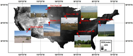
Figure 1.
Seven SURFRAD stations and the corresponding photographs.
In addition to SURFRAD in situ data located in the US, we also used Heihe in situ data located in China to explore whether this method can be applied to other regions except for the US. The Heihe in situ data is provided by the Watershed Allied Telemetry Experimental Research (WATER) project. These Heihe sites are in the Heihe River basin, which is located in the arid area of Northwest China, and the measures are collected every 10 minutes [63,64]. Both SURFRAD and Heihe measurements need to be processed before use, that is, we needed to convert all the sites’ outgoing and incoming radiation into LST by implementing the following equation.
where is the measured upwelling longwave radiation, is the measured downwelling longwave radiation, is the Stefan-Boltzmann constant (), and is the surface broadband emissivity, which can be estimated from the narrowband to broadband linear conversion method as follows:
where , , and are the narrow-band emissivities of MODIS bands 29, 31, and 32, respectively.
In the above data, LST, GOES, NDVI, albedo, DSR and SURFRAD data were used in the method calculation and accuracy assessment, and Himawari, AMSR2 and Heihe data were used in the result comparison and discussion.
2.2. Methods
As shown in Figure 2, this study used a multiple linear regression method to convert clear-sky LST to cloudy-sky LST. We used the SURFRAD site LST as the dependent variable and normalized the clear-sky LST, cloud-cover duration, downward shortwave radiation, albedo, and NDVI as the five independent variables for multiple linear regression. We selected the Bayesian maximum entropy (BME) algorithm as the clear-sky LST reconstruction algorithm, filled the gaps in the daily MODIS LST (cloud pixels identified by the MODIS QC), and obtained the spatially continuous clear-sky LST of the United States in 2015 and 2016. The BME clear-sky LST reconstruction method required the input of hard data, soft data with uncertainty, and covariance model into the BME algorithm. We took the difference of MODIS observed LST minus the mean LST of 15 days (the nearest 7 days before and after the target day) as the hard data input, and the LST Gaussian distribution constructed by auxiliary information such as elevation as the soft data input (the mean value of this Gaussian distribution also needed to subtract the mean LST of 15 days), and then calculated the daily spatial covariance coefficients. Finally, we input these three data into the BME model and obtained the reconstructed BME clear-sky LST. The specific calculation process followed that of Zhang [37]. In addition to the clear-sky LST, we also selected the cloud-cover duration and downward shortwave radiation as independent variables to consider the impact of atmospheric disturbances on the real LST and selected albedo and NDVI as the independent variables to consider the effect of surface properties on the real LST. Previous studies usually employ only downward shortwave radiation to consider the impact of atmospheric disturbances on real LST. Since we wanted to explore whether the cloud-cover duration before the MODIS observation moment can affect the real LST, the atmospheric disturbance factor of the cloud-cover duration was added, which could also reflect the duration of solar radiation. Calculating the cloud-cover duration requires geostationary satellite data with high temporal resolution. In this paper, the QC data of the GOSE hourly LST product were used, which can identify whether the target pixel has cloud cover in each hour. Since the LST to be reconstructed in this paper was in the daytime, we used the MODIS LST observation time of the target pixel to subtract its sunrise time and then combined the GOES data to determine the number of hours of cloud cover during this period. The formula for calculating sunrise time is as follows:
where denotes the sunset time, which is calculated by substituting formulas 3 and 4 into formula 5. and are solar correction and solar declination, and are longitude and latitude, denotes UTC offset, and is day of year (DOY, number of days since 1 January). It is worth noting that considering the availability of data and the simplicity of method processing, this study made the following assumptions: (1) the LST from the SURFRAD points can represent the LST of MODIS 1 km pixels; (2) the DSR and geostationary satellite products resampled from 5 km to 1 km can meet the accuracy requirements; (3) the pixels surrounding the target pixel that were used to calculate the clear-sky LST independent variable were in the clear-sky conditions from sunrise to the observation time.
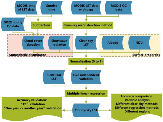
Figure 2.
Flowchart of the cloudy-sky LST calculation model and accuracy assessment.
This study adopted two methods to verify the accuracy: (1) we randomly divided the 2015 or 2016 data into a training set and a validation set with a ratio of 3:1 and used the training dataset to calculate the regression model parameters and the validation dataset to test the regression results, which was later referred to as the “3:1” validation. (2) We used all the data in 2016 to obtain the regression model parameters and apply them to the data in 2015, which we later referred to as the “2016->2015” validation. Similarly, we used the 2015 data as the training set and the 2016 data as the validation set, which we called the “2015-> 2016” validation.
To better understand the results and make better use of the method in the future, we displayed the results and compared the precision among different cases. To determine the effect of the five independent variables on the real LST and in order to simplify the method further, we analyzed the contribution of 5 variables to the real LST. Then, we discussed the accuracy of the results with the use of the two different clear-sky LST reconstruction methods and another intelligent regression algorithm (cubic support vector machines), which can provide insights into the flexibility of this method. Finally, we applied this method in China to examine the applicability of this method in other regions.
3. Results
3.1. Accuracy Assessment
We calculated the data for 2015 and 2016 in the United States to obtain the results and verify their accuracy. Figure 3 and Figure 4 show some relevant accuracy validations of all SURFRAD site data in 2015 and 2016, respectively, and N represents the number of data points involved. Under clear-sky conditions, the mean absolute error (MAE) between the MODIS-observed LST and the SURFRAD LST was 2.49 k in 2015 and 2.65 k in 2016, with an MAE value close to 2.6 K (Figure 3a, Figure 4a). This value can be regarded as the original maximum accuracy that can be achieved under ideal conditions, that is, in the presence of clouds, neither the reconstructed clear-sky LST nor the calculated real LST can be higher than this accuracy. After that, we covered the MODIS observations of the pixels in Figure 3a and Figure 4a, that is, assuming that the MODIS observed LST of these pixels were unknown, then we used the BME clear-sky reconstruction method to estimate the LST of the covered pixels. This estimated LST was called the ‘BME clear-sky LST in clear-sky condition’ in Figure 3b,c and Figure 4b,c. Figure 3b and Figure 4b show the scatter plots between the reconstructed BME clear-sky LST in clear-sky condition and the MODIS observed LST, which shows that the MAE conformed to the BME algorithm accuracy of approximately 0.5 K. Next, we calculated the MAE between the reconstructed BME clear-sky LST in the clear-sky condition and SURFRAD LST (Figure 3c, Figure 4c), whose value was very close to the values in Figure 3a and Figure 4a, which indicated that the chosen BME clear-sky LST reconstruction algorithm had high accuracy under clear-sky conditions and could support us in further calculating the real LST. Then, we selected the pixels that had no MODIS observations under cloudy conditions and used the BME method to reconstruct the LST, which was called the “BME clear-sky LST in cloudy-sky condition”. Figure 3d and Figure 4d show that the MAE between the BME clear-sky LST in cloudy-sky condition and the SURFRAD LST was close to 5.2 K. It can be seen that in actual cloudy conditions, the reconstructed LST using the clear-sky method had a large error, which was approximately twice that of Figure 3c and Figure 4c. It is necessary to convert these LST into real cloudy-sky LST, which was more consistent with the real LST. As described in the methods section, we used the BME-reconstructed LST and the other four factors as the independent variables, took SURFRAD LST as the dependent variable to establish a regression relationship, and then used this regression relationship to obtain the real LST of all cloud pixels. It was called the regression cloudy-sky LST in the figures. Figure 3e and Figure 4e present the “3:1” validation results for 2015 and 2016, respectively. As mentioned before, the “3:1” validation was to split data of one year randomly into training and validation datasets with a ratio of 3:1. The training set was used for method parameter calculation, and the validation set was used for accuracy verification. The MAE between the regression cloudy-sky LST and the SURFRAD LST obtained from the “3:1” validation was 3.52 k in 2015 and 3.54 k in 2016. When the 2016 data were used as the training set for method parameter calculation and the 2015 data as the validation set for accuracy verification, the validation accuracy was 3.86 K (Figure 3f). Similarly, when the 2015 data were used as the training set and the 2016 data as the validation set, the validation accuracy was 3.88 K (Figure 4f).
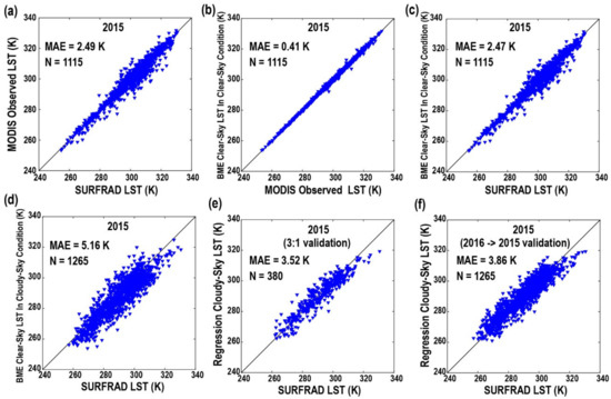
Figure 3.
Scatter plots in 2015 of (a) Moderate Resolution Imaging Spectroradiometer (MODIS) observed LST versus SURFRAD LST, (b) Bayesian maximum entropy (BME) clear-sky LST in clear-sky condition versus MODIS observed LST, (c) BME clear-sky LST in clear-sky condition versus SURFRAD LST, (d) BME clear-sky LST in cloudy-sky condition versus SURFRAD LST, (e) regression cloudy-sky LST versus SURFRAD LST (data from 2015 were randomly split into training and validation datasets at a ratio of 3:1), and (f) regression cloudy-sky LST versus SURFRAD LST (data from 2016 were used for training datasets and 2015 data for validation datasets).
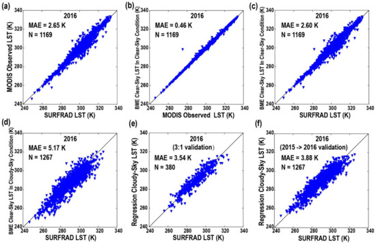
Figure 4.
Scatter plots in 2016 of (a) MODIS observed LST versus SURFRAD LST, (b) BME clear-sky LST in clear-sky condition versus MODIS observed LST, (c) BME clear-sky LST in clear-sky condition versus SURFRAD LST, (d) BME clear-sky LST in cloudy-sky condition versus SURFRAD LST, (e) regression cloudy-sky LST versus SURFRAD LST (data from 2016 were randomly split into training and validation datasets at a ratio of 3:1), and (f) regression cloudy-sky LST versus SURFRAD LST (data from 2015 were used for training datasets and 2016 data for validation datasets).
Figure 5 and Figure 6 show the bias and MAE of each SURFRAD station in 2015 and 2016 using box and line charts. On each box, the central mark indicates the median, and the bottom and top edges of the box indicate the 25th and 75th percentiles, respectively, and the outliers are plotted individually using the ‘+’ symbol. The meanings of the six subgraphs in Figure 5 correspond to those in Figure 3, and the meanings of the six subgraphs in Figure 6 correspond to those in Figure 4. The difference between these graphs is that Figure 3 and Figure 4 show the total results of the seven SURFRAD sites, while Figure 5 and Figure 6 show the results of each site of the seven SURFRAD sites.
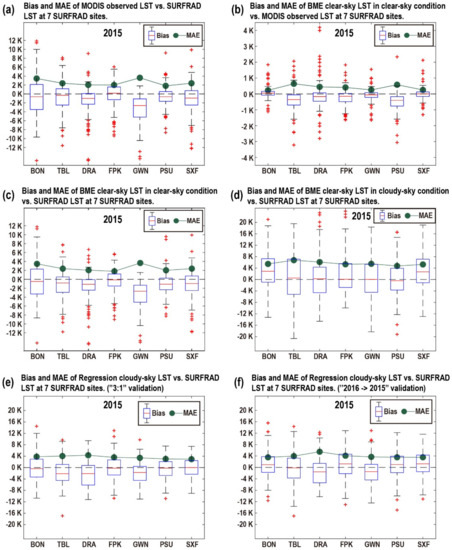
Figure 5.
Bias and mean absolute error (MAE) of (a) MODIS observed LST versus SURFRAD LST, (b) BME clear-sky LST in clear-sky condition versus MODIS observed LST, (c) BME clear-sky LST in clear-sky condition versus SURFRAD LST, (d) BME clear-sky LST in cloudy-sky condition versus SURFRAD LST, (e) regression cloudy-sky LST versus SURFRAD LST (data from 2015 were randomly split into training and validation datasets at the ratio of 3:1), and (f) regression cloudy-sky LST versus SURFRAD LST (data from 2016 were used for training datasets and 2015 data for validation datasets) at 7 SURFRAD sites in 2015.
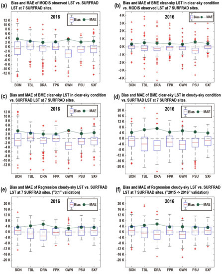
Figure 6.
Bias and MAE of (a) MODIS observed LST versus SURFRAD LST, (b) BME clear-sky LST in clear-sky condition versus MODIS LST, (c) BME clear-sky LST in clear-sky condition versus SURFRAD LST, (d) BME clear-sky LST in cloudy-sky condition versus SURFRAD LST, (e) regression cloudy-sky LST versus SURFRAD LST (data from 2016 were randomly split into training and validation datasets at the ratio of 3:1), and (f) regression cloudy-sky LST versus SURFRAD LST (data from 2015 were used for training datasets and 2016 data for validation datasets) at 7 SURFRAD sites in 2016.
In general, under clear-sky conditions, the LST reconstructed by the clear-sky LST algorithm had high accuracy, which can be comparable to the direct observations of MODIS (Figure 5a,c, Figure 6a,c). In the presence of clouds, the clear-sky LST reconstruction algorithm had a large error (Figure 5d, Figure 6d). The accuracy of the real LST obtained by the multiple linear regression method in this paper was significantly improved compared with the LST directly estimated by the clear-sky algorithm, but it cannot reach the accuracy of the clear-sky algorithm under clear-sky conditions (Figure 5e,f, Figure 6e,f).
An interesting aspect we noticed was that under clear-sky conditions, the accuracy of the reconstructed LST at site Desert Rock (DRA) was high, reaching approximately 2 K (Figure 5c, Figure 6c), while the error of BME clear-sky LST in cloudy-sky condition was very large, exceeding 6 K (Figure 5d) in 2015 and 7 K (Figure 6d) in 2016. The obtained real LST after multiple linear regression also had the lowest accuracy for all seven sites. Its MAE at this time was approximately 5.5 K, and there was serious underestimation. DRA’s land-cover type was the only barren area among the seven sites, and LST reconstruction methods usually had lower accuracy in barren surface.
The other two sites with large real LST errors after regression were Fort Peck (FPK) in 2015 and Table Mountain (TBL) in 2016, the MAE of which both exceed 4 K (Figure 5f, Figure 6f), while under clear-sky conditions, the MAE between the MODIS observed LST and the measured real LST did not exceed 3 K (Figure 5a, Figure 6a). The MAE between Goodwin Creek’s (GWN) MODIS-observed LST and real LST was approximately 3.6 K (Figure 5a, Figure 6a), which was the largest among the seven sites. But the MAE after performing multiple linear regression was approximately 3.7 K, which was close to 3.6 K.
Under cloudy conditions, except for the sites DRA and FPK in 2015 and DRA and TBL in 2016, the MAEs between the regression LST and the measured real LST at the other sites ranged from 3.2 K–3.9 K.
3.2. Independent Variable Analysis
Table 2 displays the Pearson correlation coefficient between the five independent variables. The clear-sky LST and DSR, clear-sky LST and albedo, clear-sky and NDVI showed moderate correlations, and there was a weak or very weak correlation between the remaining variables. There was no strong correlation or extremely strong correlation between all independent variables. Therefore, it is reasonable to use these five independent variables for multiple linear regression.
Table 2.
Pearson correlation coefficients between 5 independent variables.
Before performing multiple linear regression, all independent variables should be normalized so that their values range from 0 to 1. The second and third columns of Table 3 show the minimum and maximum values used to normalize the five independent variables, which were basically equal to the effective value range of the corresponding remote sensing products. All calculated coefficients of the multiple linear regressions for 2015 and 2016 are illustrated in columns 4 and 5 of Table 3, respectively. We provide the normalization parameters and regression coefficients for the convenience of reuse in future studies.
Table 3.
Maximum and minimum values used for normalization and multiple linear regression coefficients in 2015 and 2016.
Since the variables were normalized to 0–1, we can get from the coefficients that the contribution of each independent variable to the real LST. The contribution can be sorted from large to small as: clear-sky LST > DSR > Albedo > NDVI > cloud-cover duration. Cloud-cover duration and NDVI contributed the least to the results, up to 1.69 K and 4.29 K, respectively (Table 3). When we only selected the four independent variables of clear-sky LST, DSR, Albedo and NDVI, the accuracy obtained was very close to that of selecting the five variables. When we only selected the three independent variables of clear-sky LST, DSR, and Albedo, the MAE was also less than 4 K.
3.3. Accuracy Comparison under Different Conditions
3.3.1. Accuracy Comparison with Different Clear-Sky Land-Surface Temperature (LST) Reconstruction Methods
This paper selected the BME algorithm when reconstructing clear-sky LST independent variables. However, there are many other clear-sky LST algorithms. Therefore, we also explored the effect of clear-sky LSTs reconstructed by other methods on the regression accuracy of the real LST. Due to the low accuracy of the time interpolation algorithm used to reconstruct the clear-sky LST, we selected the kriging spatial interpolation algorithm and the hybrid gapfilling method proposed by Li [31], both of which are popular and have relatively high accuracy. We kept the other 4 independent variables unchanged and replaced the BME clear-sky LST with the clear-sky LST reconstructed by the other two methods (kriging and Li’s gapfilling) and performed an accuracy comparison after multiple linear regression.
The first set of histograms in Figure 7a,b compare the accuracy of the LST reconstructed by three clear-sky algorithms under cloudy conditions in 2015 and 2016, respectively. In 2015, the MAEs between the clear-sky LST in cloudy-sky condition and SURFRAD LST calculated by BME, kriging, and gapfilling were 5.16 K, 5.38 K, and 9.33 K, respectively. In 2016, the corresponding MAEs were 5.17 K, 5.36 K, and 7.60 K. This result suggested that the errors between the real LST sites and the LST calculated by the clear-sky LST methods were large. Then, we took the LST reconstructed by the three clear-sky algorithms as the independent variable and combined it with the other 4 independent variables to perform multiple linear regression. The “3:1” validation and the two-year interactive validation are illustrated in the second and third histograms of Figure 7a,b. In 2015, the “3:1” validation MAEs of the BME, kriging, and gapfilling regression LSTs were 3.52 K, 3.55 K, 4.88 K, and the corresponding MAEs in 2016 were 3.54 K, 3.60 K, 4.75 K, respectively. The MAEs of the two-year interactive validation were slightly higher than the values of the “3:1” validation. Therefore, for the estimation of the clear-sky LST independent variable, the MAE of the regression LST was less than 4 K when selecting the kriging or BME method and greater than 4 K when choosing the gapfilling method.
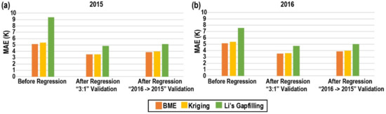
Figure 7.
Comparison of the influence of three different clear-sky LST reconstruction methods on the accuracy of regression cloudy-sky LST in 2015 (a) and in 2016 (b).
3.3.2. Accuracy Comparison with Different Regression Methods
This paper used the most basic multiple linear regression method as the core method. In fact, there are currently a large number of intelligent regression tools. The regression learner app in MATLAB can train regression models to predict data. It is simple and convenient to operate. The regression model types in this app include linear regression models, regression trees, support vector machines (SVM), Gaussian process regression models, and ensembles of regression trees. We input the independent and dependent variables into the app and performed automated training to search for the best regression model type. The results showed that cubic SVM regression performed best among all regression models. Therefore, we compared the cubic SVM regression model with the multiple linear regression used in this paper. Intelligent regression usually uses five-fold cross validation for accuracy verification, and we compared it to the “3:1” validation of the multiple linear regression. In 2015, the MAEs between the multiple linear regression LST and SURFRAD LST and cubic SVM regression LST and SURFRAD LST were 3.52 K and 3.43 K, respectively. The corresponding MAEs in 2016 were 3.54 K and 3.38 K (Figure 8). The “3:1” validation and five-fold cross validation for these comparisons indicated that the cubic SVM regression improved accuracy over the multiple linear regression by 0.1–0.16 K. When the 2016 data were used as the training set and the 2015 data as the validation set, the MAEs of the multiple linear regression and cubic SVM regression were 3.86 K and 3.87 K. Similarly, when the coefficients obtained in 2015 were applied to 2016, the corresponding two MAEs were 3.88 K and 3.80 K. This two-year interactive validation indicated that the cubic SVM regression tool basically did not improve the accuracy.
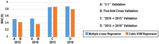
Figure 8.
Comparison of the accuracy of two different regression tools (multiple linear regression and cubic support vector machines (SVM) regression).
3.3.3. Accuracy Comparison in Different Regions
In addition, we want to investigate whether this method is applicable to other regions except the United States. Another research area we selected was the Heihe region in Northwest China, which also had ground observations of longwave radiation. The SURFRAD data were replaced as the dependent variable by the Heihe data, and the GOES data for calculating the cloud-cover duration variable were replaced with Himawari data to cover the Heihe area. There were 4 available Heihe stations for 2016, of which two were removed because the MAE between their measured LST and MODIS-observed LST exceeded 5 K. The land-cover types of the remaining two effective Heihe sites were forest and reed wetlands. Figure 9 shows the various accuracy validations of the Heihe region. Under clear-sky conditions, the MAE between the MODIS observations and the Heihe measurement was 3.93 K (Figure 9a), indicating that the measured LST of the Heihe site itself had high error. The MAE between the reconstructed BME clear-sky LST in clear-sky condition and the Heihe LST reached 4.23 K, exceeding 4 K (Figure 9c). Under cloudy conditions, the MAE between the LST reconstructed by the BME method and the LST measured at Heihe was 5.69 K (Figure 9d). After conducting the multiple linear regression in this paper, the accuracy of the “3:1” validation was 3.34 K, which did not exceed 4 K (Figure 9e). This MAE was smaller than the MAE shown in Figure 9a, which may be due to the low accuracy of the Heihe station itself, resulting in a certain degree of over-regression. When the Heihe data in 2016 were used as the training set for method parameter calculation and the 2015 data as the validation set for accuracy verification, the validation accuracy was 3.96 K, which also did not exceed 4 K (Figure 9f). Finally, we directly applied the regression coefficients of the US region in 2016 to the Heihe region, and the obtained MAE between the real LST and the LST measured at Heihe was up to 5.4 K (Figure 9g), although this MAE was 0.3 k lower than that in Figure 9d, and the point distribution was significantly more concentrated towards the 1:1 line. The results suggested that the conversion method in this paper had a certain cross-regional capability, and it is better to use the local site data to recalculate the regression coefficients when using this method in other regions outside the United States.
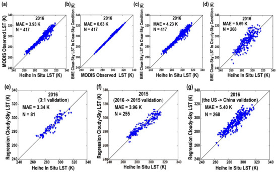
Figure 9.
Scatter plots in 2016 of (a) MODIS-observed LST versus Heihe in situ LST, (b) BME clear-sky LST in clear-sky condition versus MODIS observed LST, (c) BME clear-sky LST in clear-sky condition versus Heihe in situ LST, (d) BME clear-sky LST in cloudy-sky condition versus Heihe in situ LST, (e) regression cloudy-sky LST versus Heihe in situ LST (data from 2016 were randomly split into training and validation datasets at a ratio of 3:1), (f) regression cloudy-sky LST versus Heihe in situ LST (data from 2016 were used for training datasets and 2015 data for validation datasets), and (g) regression cloudy-sky LST versus Heihe in situ LST (applying the 2016 regression coefficients in the US to China).
3.4. Spatial Patterns of the Cloudy-Sky LSTs
We selected the MODIS images from 29 April 2015; 12 October 2015; 20 July 2016 and 4 November 2016 and ran the BME algorithm to fill the clear-sky LST and used the simple conversion method to reconstruct the real LST (Figure 10). The first column of Figure 10 is the original MODIS images, the second column is the LST spatial distribution after using the BME clear-sky algorithm, the third column is the spatial distribution of the real LST calculated through regression, and the fourth column shows the spatial distribution of the difference LST calculated by the real LST from the regression minus the BME-reconstructed clear-sky LST.
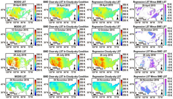
Figure 10.
Spatial distribution of MODIS LST (first column), BME clear-sky LST in cloudy-sky condition (second column), regression cloudy-sky LST (third column) and regression cloudy-sky LST minus BME clear-sky LST (fourth column) on 29 April 2015 (first row); 12 October 2015 (second row); 20 July 2016 (third row); and 4 November 2016 (fourth row).
The second and third columns of Figure 10 can reflect the spatial distribution characteristics of LST in the US. In general, the LST was higher in the north and lower in the south and higher in the west and lower in the east, while the LST at the boundary of the Rocky Mountains was lower in the west and higher in the east. The spatial heterogeneity of the LST was slightly higher in summer than in winter. Each region also had its own characteristics. The temperate climate zone in the northeast was cold in winter, the subtropical zone in the southeast was warm and humid, and the western plateau region had a large annual LST difference. The LSTs generated by the BME algorithm or regression method had both smoothness and extreme values. The spatial distribution of the difference in the fourth column of Figure 10 was generally irregular. There were more grassland and barren land-cover types with negative values, and the forest and cropland were interspersed with positive and negative values.
4. Discussion
4.1. Suggestions for Method Usage
We selected five independent variables to perform multiple linear regression to convert the clear-sky LST to real LST, resulting in a MAE ranging from approximately 3.5–3.9 K. This error was comparable to that of the previous methods. For example, the root mean square error (similar to MAE) of the cloudy-sky LST obtained by the method combining PMW and TIR data range from 3.4–4.4 K [47], and the MAE of the cloudy-sky LST retrieved by the method based on energy conservation is 3-6 K [51].
In addition to the clear-sky LST, we selected the four independent variables of cloud-cover duration, DSR, NDVI, and albedo. Among them, the cloud-cover duration factor has not been taken into account in previous studies. We considered that the instantaneous LST was closely related to the cumulative solar radiation received by the surface before the LST observation moment, and the cloud-cover duration describes this quantity to a certain extent and is relatively easy to calculate; therefore, we included the cloud-cover duration as an independent variable. However, the results showed that adding cloud-cover duration as an independent variable did not significantly improve the accuracy. This was probably because we used the spatial neighbouring pixels of the target pixel when calculating the clear-sky LST, and these neighbouring pixels also had different cloud-cover durations before the observation time. Since we had taken the clear-sky LST calculated by these adjacent pixels as the independent variable, it was of little significance to consider the cloud-cover duration of the target pixel at the same time. From the point where the regression coefficient of the cloud-cover duration was greater than zero, we can also see that considering this independent variable did not achieve the expected effect.
In the future selection of independent variables, the four independent variables of clear-sky LST, DSR, NDVI, and albedo can be selected, which can achieve good results. To further simplify the process, the three independent variables of clear-sky LST, DSR, and albedo can be chosen to achieve acceptable accuracy (MAE of less than 4 K). In this case, only the DSR was considered the influencing factor of the atmospheric disturbance on the real LST, and the effect of the surface properties on the real LST included only the albedo. Regarding the clear-sky LST reconstruction methods, we recommend algorithms with high accuracy, such as spatial or spatio-temporal gapfilling algorithms containing auxiliary information, while the time interpolation method is not recommended. Regarding the regression tools, multiple linear regression can be chosen to simplify the calculation, and intelligent regression tools such as cubic SVM regression contributes small improvements in the accuracy of the results. Regarding the research area, one can directly use the regression coefficients in this study to obtain the real LST of the United States. If another study area is selected, it is suggested that the regression relationship should be re-established and the regression coefficients should be calculated.
4.2. Analysis of Error Source and Ideal Situations
In this paper, the error sources for the method of converting clear-sky LST to cloudy-sky LST included: (1) the error caused by the inconsistency in spatial scales between the MODIS observations and SURFRAD site measurements, between the DSR and MODIS LST, and between the GOES LST and MODIS LST; (2) the clear-sky algorithm itself, which had errors when calculating the clear-sky LST independent variable; and (3) the spatial neighbourhood pixels used in estimating the target pixel, which also had different cloud-cover durations. Therefore, we consider the cloud-cover duration of only the target pixel will cause errors. This study assumed a relatively ideal situation, that is, the surrounding pixels used in calculating the clear-sky LST independent variable were all in clear-sky conditions from sunrise to the observation time, and the retrieved clear-sky LSTs of the target pixel thus should be greater than the measured real LSTs at the SURFRAD sites. This means that the theoretical LST values should be greater than the real LST values due to cloud occlusion. However, the calculated results showed that the clear-sky LSTs of approximately half of the pixels were lower than the SURFRAD site LST values, indicating that the ideal situation was not reached. If we remove the points where the clear-sky LST was less than the SURFRAD site LST, leaving only the points where the clear-sky LST was greater than the SURFRAD site LST, then we establish multiple linear regression. The regression coefficients and accuracy obtained from this situation are shown in Table 4. The accuracy in this relatively ideal situation was high. The MAE ranged from 2.3–2.5 K, which was almost as small as the MAE between the MODIS-observed LST and the SURFRAD-measured LST. Therefore, if we can find a way to take into account the cloud-cover durations of the spatial neighbourhood pixels of the target pixel, the accuracy will be greatly improved. In theory, improving the spatial resolution of variables such as DSR and improving the accuracy of the clear-sky LST algorithms can also improve the accuracy of the real LST. In addition, it can be inferred from Figure 5 and Figure 6 that regression according to different land-cover types, especially separating the barren surface from other land types with more vegetation coverage, may reduce the error. We can also try to add variables, such as temperature or soil moisture, to improve accuracy.
Table 4.
Multiple linear regression coefficients and MAEs in 2015 and 2016 when only selecting the points with clear-sky LST values greater than the SURFRAD LST.
4.3. Comparison with Advanced Microwave Scanning Radiometer 2 (AMSR2) LST
Because the SURFRAD site measurements were the only the dependent variable in this paper, it is necessary to verify whether the SURFRAD data are representative and whether the regression relationship obtained through these sites can be applied to all pixels in the United States. Microwave LST is generally considered to be close to the real LST; therefore, we randomly selected 4 days in 2015 and 2016 to compare the microwave AMSR2 LST with the real LST calculated by this paper’s method (Figure 11). The blue curve in the fourth column of Figure 11 shows the distribution of the differences between the MODIS-observed LST and the microwave LST. The corresponding MAE value was the lowest value that can be achieved; that is, regardless of the method used, the MAE between the reconstructed LST and the microwave LST will not be lower than this value. The yellow curve represents the distribution of the difference between the microwave LST and the real LST obtained by regression. We can see that the real LST converted by this paper’s method was closer than the clear-sky LST (orange curve) to the microwave LST, and the corresponding MAE was also smaller. However, in most cases, the yellow curve did not reach the proximity of the MODIS-observed LST to the microwave LST (blue curve). The LST of the SURFRAD site has a certain degree of representativeness and can basically be applied to the entire study area. This study attempted to explore the regression relationship between the real value and each influencing factor. When an increasing number of representative real LSTs with high spatial resolutions can be measured, the reliability and accuracy of this method will be improved.
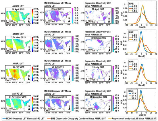
Figure 11.
Spatial distribution of the Advanced Microwave Scanning Radiometer 2 (AMSR2) LST (first column), MODIS observed LST minus AMSR2 LST (second column), regression cloudy-sky LST minus AMSR2 LST (third column), and bias distribution of MODIS LST minus AMSR2 LST, BME LST minus AMSR2 LST, regression LST minus AMSR2 LST (fourth column) on 29 April 2015 (first row), 12 October 2015 (second row), 20 July 2016 (third row), and 4 November 2016 (fourth row).
5. Conclusions
The cloudy-sky LST can better reflect the true situation of the surface than the clear-sky LST. For the 1 km daily MODIS LST product, this paper converted the clear-sky LST into the cloudy-sky LST through multiple linear regression by considering the factors of cloud-cover duration, DSR, albedo, and NDVI and taking the real LST at the SURFRAD sites as the dependent variable. The MAE of the results ranged from 3.5–3.9 K, which was close to the error of the other existing real LST reconstruction methods. We also discussed and made recommendations on the possible choices of independent variables, clear-sky algorithms, and regression tools involved in the method. Selecting three independent variables, such as clear-sky LST, DSR and albedo, for regression can also achieve satisfactory accuracy. Regarding the clear-sky algorithm, one can choose an algorithm with high accuracy that considers space and auxiliary information. For the regression tool, one can try an intelligent regression tool. This method can also be applied to other research areas. In the subsequent application, if the real LST of other years in the United States is needed, the 2015 or 2016 coefficients provided in this study can be directly selected to achieve the acceptable accuracy, or the new coefficients of the required year can be calculated to improve the accuracy.
This method has the following advantages: (1) unlike most current real LST algorithms, it does not need to find similar pixels in the space-time neighbourhood for each pixel to be estimated. (2) The variable acquisition and method construction are relatively simple. (3) This method had high flexibility in that it can apply a large number of existing clear-sky algorithms and use different regression tools.
There are also some limitations to this method: (1) The number of ground station-observed real LSTs that can be used as regression dependent variables is small; therefore, the method reliability needs to be improved. It is difficult to use this method in research areas without LST observation sites. (2) MODIS/Aqua takes two observations per day, one during the day and one at night. This method is only applicable to the situation during the day because the accuracy of the night cloudy-sky LST obtained by this method is low. (3) This method has difficulty reaching the ideal situation (the real LST is not always lower than the clear-sky LST); thus, it is difficult to improve the accuracy of the results to a great extent. (4) The method cannot quantitatively calculate the influence of the cloud-cover percentage or other factors on the uncertainty of the results.
This paper explored the regression relationship between the real LST and the various influencing factors and suggested a simple method to convert clear-sky LST into real LST. When more representative real LSTs with high spatial resolution can be measured, the usability and accuracy of the algorithm will improve. Considering that the cloud-cover duration of the LST missing pixels in this study has not received good results. Subsequent studies can try to use the high temporal resolution GOES 16 cloud data, or combine the cloud-cover duration with the LST of geostationary satellites, such as GOES and Himawari, that are observed around the MODIS acquisition time. In addition to discussing the algorithm used to convert from clear-sky LST to real LST, future studies should also continue to develop real LST algorithms based on energy conservation to increase their availability and improve the accuracy of microwave LST downscaling and gapfilling.
Author Contributions
Conceptualization, Y.Z. and Y.C.; Data curation, Y.Z. and X.C.; Formal analysis, Y.Z. and Y.C.; Funding acquisition, J.L.; Investigation, Y.Z.; Methodology, Y.Z.; Project administration, Y.C. and J.L.; Software, Y.Z. and X.C.; Supervision, Y.C. and J.L.; Validation, Y.Z.; Visualization, Y.Z.; Writing – original draft, Y.Z.; Writing – review and editing, Y.Z., Y.C., J.L. and X.C. All authors have read and agreed to the published version of the manuscript.
Funding
This work was supported by National Key R&D Program of China under Grant 2019YFC1520800, 2017YFC1502406, Projects of Beijing Advanced Innovation Center for Future Urban Design, Beijing University of Civil Engineering and Architecture (UDC2019031321), Beijing Natural Science Foundation under Grant 8192025 and in part by Beijing Laboratory of Water Resources Security.
Acknowledgments
We would like to thank the DSR data support from “National Earth System Science Data Sharing Infrastructure, National Science and Technology Infrastructure of China” (http://www.geodata.cn), and the MODIS data support from Level-1 and Atmosphere Archive and Distribution System (LAADS) Distributed Active Archive Center (DAAC) of the National Aeronautics and Space Administration (NASA). The Heihe data set was provided by “Heihe Plan Science Data Center, National Natural Science Foundation of China” (http://www.heihedata.org). The GOES and Himawari hourly LST data were available through the GlobTemperature portal, which is the LST product used by Copernicus Global Land Service (http://land.copernicus.eu/global/products/lst). The AMSR2 product was supplied by the GCOM-W Research Product Distribution Service, Japan Aerospace Exploration Agency (JAXA). We are very grateful to editors and anonymous reviewers for their insightful comments and substantial help on improving this article.
Conflicts of Interest
The authors declare no conflict of interest.
References
- Kustas, W.; Anderson, M. Advances in thermal infrared remote sensing for land surface modeling. Agric. For. Meteorol. 2009, 149, 2071–2081. [Google Scholar] [CrossRef]
- Li, Z.-L.; Tang, B.-H.; Wu, H.; Ren, H.; Yan, G.; Wan, Z.; Trigo, I.F.; Sobrino, J.A. Satellite-derived land surface temperature: Current status and perspectives. Remote Sens. Environ. 2013, 131, 14–37. [Google Scholar] [CrossRef]
- Phan, T.N.; Kappas, M. Application of MODIS land surface temperature data: A systematic literature review and analysis. J. Appl. Remote Sens. 2018, 12, 041501. [Google Scholar] [CrossRef]
- Gillespie, A.R.; Matsunaga, T.; Rokugawa, S.; Hook, S.J. Temperature and emissivity separation from advanced spaceborne thermal emission and reflection radiometer (ASTER) images. In Proceedings of the Infrared Spaceborne Remote Sensing IV, SPIE’s 1996 International Symposium on Optical Science, Engineering, and Instrumentation, Denver, CO, USA, 4–9 August 1996; SPIE: Bellingham, WA USA, 1996; pp. 82–94. [Google Scholar]
- Roy, D.P.; Wulder, M.A.; Loveland, T.R.; Woodcock, C.E.; Allen, R.G.; Anderson, M.C.; Helder, D.; Irons, J.R.; Johnson, D.M.; Kennedy, R.; et al. Landsat-8: Science and product vision for terrestrial global change research. Remote Sens. Environ. 2014, 145, 154–172. [Google Scholar] [CrossRef]
- Wan, Z. Collection-5 MODIS Land Surface Temperature Products Users’ Guide; ICESS, University of California: Santa Barbara, CA, USA, 2007. [Google Scholar]
- Jiang, G.M.; Li, Z.L. Split-window algorithm for land surface temperature estimation from MSG1-SEVIRI data. Int. J. Remote Sens. 2008, 29, 6067–6074. [Google Scholar] [CrossRef]
- Cavalieri, D.; Markus, T.; Comiso, J. AMSR-E/Aqua Daily L3 25 km Brightness Temperature & Sea Ice Concentration Polar Grids; Version 3; NASA National Snow and Ice Data Center Distributed Active Archive Center: Boulder, CO, USA, 2014.
- Kalma, J.D.; McVicar, T.R.; McCabe, M.F. Estimating Land Surface Evaporation: A Review of Methods Using Remotely Sensed Surface Temperature Data. Surv. Geophys. 2008, 29, 421–469. [Google Scholar] [CrossRef]
- Mallick, K.; Bhattacharya, B.K.; Patel, N.K. Estimating volumetric surface moisture content for cropped soils using a soil wetness index based on surface temperature and NDVI. Agric. For. Meteorol. 2009, 149, 1327–1342. [Google Scholar] [CrossRef]
- Piles, M.; Camps, A.; Vall-llossera, M.; Corbella, I.; Panciera, R.; Rudiger, C.; Kerr, Y.H.; Walker, J. Downscaling SMOS-Derived Soil Moisture Using MODIS Visible/Infrared Data. IEEE Trans. Geosci. Remote Sens. 2011, 49, 3156–3166. [Google Scholar] [CrossRef]
- Vancutsem, C.; Ceccato, P.; Dinku, T.; Connor, S.J. Evaluation of MODIS land surface temperature data to estimate air temperature in different ecosystems over Africa. Remote Sens. Environ. 2010, 114, 449–465. [Google Scholar] [CrossRef]
- Benali, A.; Carvalho, A.C.; Nunes, J.P.; Carvalhais, N.; Santos, A. Estimating air surface temperature in Portugal using MODIS LST data. Remote Sens. Environ. 2012, 124, 108–121. [Google Scholar] [CrossRef]
- Zhu, W.; Lű, A.; Jia, S. Estimation of daily maximum and minimum air temperature using MODIS land surface temperature products. Remote Sens. Environ. 2013, 130, 62–73. [Google Scholar] [CrossRef]
- Kloog, I.; Nordio, F.; Coull, B.A.; Schwartz, J. Predicting spatiotemporal mean air temperature using MODIS satellite surface temperature measurements across the Northeastern USA. Remote Sens. Environ. 2014, 150, 132–139. [Google Scholar] [CrossRef]
- Bisht, G.; Bras, R.L. Estimation of net radiation from the MODIS data under all sky conditions: Southern Great Plains case study. Remote Sens. Environ. 2010, 114, 1522–1534. [Google Scholar] [CrossRef]
- Wu, C.; Munger, J.W.; Niu, Z.; Kuang, D. Comparison of multiple models for estimating gross primary production using MODIS and eddy covariance data in Harvard Forest. Remote Sens. Environ. 2010, 114, 2925–2939. [Google Scholar] [CrossRef]
- Imhoff, M.L.; Zhang, P.; Wolfe, R.E.; Bounoua, L. Remote sensing of the urban heat island effect across biomes in the continental USA. Remote Sens. Environ. 2010, 114, 504–513. [Google Scholar] [CrossRef]
- Schwarz, N.; Lautenbach, S.; Seppelt, R. Exploring indicators for quantifying surface urban heat islands of European cities with MODIS land surface temperatures. Remote Sens. Environ. 2011, 115, 3175–3186. [Google Scholar] [CrossRef]
- Rhee, J.; Im, J.; Carbone, G.J. Monitoring agricultural drought for arid and humid regions using multi-sensor remote sensing data. Remote Sens. Environ. 2010, 114, 2875–2887. [Google Scholar] [CrossRef]
- Amani, M.; Salehi, B.; Mahdavi, S.; Masjedi, A.; Dehnavi, S. Temperature-Vegetation-soil Moisture Dryness Index (TVMDI). Remote Sens. Environ. 2017, 197, 1–14. [Google Scholar] [CrossRef]
- Xu, H. A remote sensing index for assessment of regional ecological changes. China Environ. Sci. 2013, 33, 889–897. [Google Scholar]
- Garuma, G.F.; Blanchet, J.-P.; Girard, É.; Leduc, M. Urban surface effects on current and future climate. Urban Clim. 2018, 24, 121–138. [Google Scholar] [CrossRef]
- Pede, T.; Mountrakis, G. An empirical comparison of interpolation methods for MODIS 8-day land surface temperature composites across the conterminous Unites States. ISPRS J. Photogramm. Remote Sens. 2018, 142, 137–150. [Google Scholar] [CrossRef]
- Crosson, W.L.; Al-Hamdan, M.Z.; Hemmings, S.N.J.; Wade, G.M. A daily merged MODIS Aqua–Terra land surface temperature data set for the conterminous United States. Remote Sens. Environ. 2012, 119, 315–324. [Google Scholar] [CrossRef]
- Xu, Y.; Shen, Y. Reconstruction of the land surface temperature time series using harmonic analysis. Comput. Geosci. 2013, 61, 126–132. [Google Scholar] [CrossRef]
- Kang, J.; Tan, J.; Jin, R.; Li, X.; Zhang, Y. Reconstruction of MODIS Land Surface Temperature Products Based on Multi-Temporal Information. Remote Sens. 2018, 10, 1112. [Google Scholar] [CrossRef]
- Weiss, D.J.; Atkinson, P.M.; Bhatt, S.; Mappin, B.; Hay, S.I.; Gething, P.W. An effective approach for gap-filling continental scale remotely sensed time-series. ISPRS J. Photogramm. Remote Sens. 2014, 98, 106–118. [Google Scholar] [CrossRef]
- Zeng, C.; Shen, H.; Zhong, M.; Zhang, L.; Wu, P. Reconstructing MODIS LST Based on Multitemporal Classification and Robust Regression. IEEE Geosci. Remote Sens. Lett. 2015, 12, 512–516. [Google Scholar] [CrossRef]
- Sun, L.; Chen, Z.; Gao, F.; Anderson, M.; Song, L.; Wang, L.; Hu, B.; Yang, Y. Reconstructing daily clear-sky land surface temperature for cloudy regions from MODIS data. Comput. Geosci. 2017, 105, 10–20. [Google Scholar] [CrossRef]
- Li, X.; Zhou, Y.; Asrar, G.R.; Zhu, Z. Creating a seamless 1km resolution daily land surface temperature dataset for urban and surrounding areas in the conterminous United States. Remote Sens. Environ. 2018, 206, 84–97. [Google Scholar] [CrossRef]
- Pham, H.T.; Kim, S.; Marshall, L.; Johnson, F. Using 3D robust smoothing to fill land surface temperature gaps at the continental scale. Int. J. Appl. Earth Obs. Geoinf. 2019, 82, 101879. [Google Scholar] [CrossRef]
- Yang, J.; Wang, Y.; August, P. Estimation of land surface temperature using spatial interpolation and satellite-derived surface emissivity. J. Environ. Inform. 2004, 4, 37–44. [Google Scholar] [CrossRef]
- Neteler, M. Estimating Daily Land Surface Temperatures in Mountainous Environments by Reconstructed MODIS LST Data. Remote Sens. 2010, 2. [Google Scholar] [CrossRef]
- Ke, L.; Ding, X.; Song, C. Reconstruction of Time-Series MODIS LST in Central Qinghai-Tibet Plateau Using Geostatistical Approach. IEEE Geosci. Remote Sens. Lett. 2013, 10, 1602–1606. [Google Scholar] [CrossRef]
- Metz, M.; Rocchini, D.; Neteler, M. Surface Temperatures at the Continental Scale: Tracking Changes with Remote Sensing at Unprecedented Detail. Remote Sens. 2014, 6. [Google Scholar] [CrossRef]
- Zhang, Y.; Chen, Y.; Li, Y.; Xia, H.; Li, J. Reconstructing One Kilometre Resolution Daily Clear-Sky LST for China’s Landmass Using the BME Method. Remote Sens. 2019, 11, 2610. [Google Scholar] [CrossRef]
- Wu, P.; Shen, H.; Zhang, L.; Göttsche, F.-M. Integrated fusion of multi-scale polar-orbiting and geostationary satellite observations for the mapping of high spatial and temporal resolution land surface temperature. Remote Sens. Environ. 2015, 156, 169–181. [Google Scholar] [CrossRef]
- Kebiao, M.; Jiancheng, S.; Zhaoliang, L.; Zhihao, Q.; Yuanyuan, J. Land surface temperature and emissivity retrieved from AMSR passive micro-wave data. In Proceedings of the 2005 IEEE International Geoscience and Remote Sensing Symposium (IGARSS ’05), Seoul, Korea, 29–29 July 2005; pp. 2247–2249. [Google Scholar]
- Mao, K.; Shi, J.; Li, Z.; Qin, Z.; Li, M.; Xu, B. A physics-based statistical algorithm for retrieving land surface temperature from AMSR-E passive microwave data. Sci. China Ser. D Earth Sci. 2007, 50, 1115–1120. [Google Scholar] [CrossRef]
- Yuan-Yuan, J.; Bohui, T.; Xiaoyu, Z.; Zhao-Liang, L. Estimation of land surface temperature and emissivity from AMSR-E data. In Proceedings of the 2007 IEEE International Geoscience and Remote Sensing Symposium, Barcelona, Spain, 23–28 July 2007; pp. 1849–1852. [Google Scholar]
- Gao, H.; Fu, R.; Dickinson, R.E.; Juarez, R.I.N. A Practical Method for Retrieving Land Surface Temperature From AMSR-E Over the Amazon Forest. IEEE Trans. Geosci. Remote Sens. 2008, 46, 193–199. [Google Scholar] [CrossRef]
- Holmes, T.R.H.; De Jeu, R.A.M.; Owe, M.; Dolman, A.J. Land surface temperature from Ka band (37 GHz) passive microwave observations. J. Geophys. Res. Atmos. 2009, 114. [Google Scholar] [CrossRef]
- Zhao, E.; Gao, C.; Jiang, X.; Liu, Z. Land surface temperature retrieval from AMSR-E passive microwave data. Opt. Express 2017, 25, A940–A952. [Google Scholar] [CrossRef]
- Kou, X.; Jiang, L.; Bo, Y.; Yan, S.; Chai, L. Estimation of Land Surface Temperature through Blending MODIS and AMSR-E Data with the Bayesian Maximum Entropy Method. Remote Sens. 2016, 8. [Google Scholar] [CrossRef]
- Shwetha, H.R.; Kumar, D.N. Prediction of high spatio-temporal resolution land surface temperature under cloudy conditions using microwave vegetation index and ANN. ISPRS J. Photogramm. Remote Sens. 2016, 117, 40–55. [Google Scholar] [CrossRef]
- Duan, S.-B.; Li, Z.-L.; Leng, P. A framework for the retrieval of all-weather land surface temperature at a high spatial resolution from polar-orbiting thermal infrared and passive microwave data. Remote Sens. Environ. 2017, 195, 107–117. [Google Scholar] [CrossRef]
- Sun, D.; Li, Y.; Zhan, X.; Houser, P.; Yang, C.; Chiu, L.; Yang, R. Land Surface Temperature Derivation under All Sky Conditions through Integrating AMSR-E/AMSR-2 and MODIS/GOES Observations. Remote Sens. 2019, 11, 1704. [Google Scholar] [CrossRef]
- Xu, S.; Cheng, J.; Zhang, Q. Reconstructing All-Weather Land Surface Temperature Using the Bayesian Maximum Entropy Method Over the Tibetan Plateau and Heihe River Basin. IEEE J. Sel. Top. Appl. Earth Obs. Remote Sens. 2019, 12, 3307–3316. [Google Scholar] [CrossRef]
- Jin, M.; Dickinson, R.E. A generalized algorithm for retrieving cloudy sky skin temperature from satellite thermal infrared radiances. J. Geophys. Res. Atmos. 2000, 105, 27037–27047. [Google Scholar] [CrossRef]
- Zeng, C.; Long, D.; Shen, H.; Wu, P.; Cui, Y.; Hong, Y. A two-step framework for reconstructing remotely sensed land surface temperatures contaminated by cloud. ISPRS J. Photogramm. Remote Sens. 2018, 141, 30–45. [Google Scholar] [CrossRef]
- Yang, G.; Sun, W.; Shen, H.; Meng, X.; Li, J. An Integrated Method for Reconstructing Daily MODIS Land Surface Temperature Data. IEEE J. Sel. Top. Appl. Earth Obs. Remote Sens. 2019, 12, 1026–1040. [Google Scholar] [CrossRef]
- Yu, W.; Tan, J.; Ma, M.; Li, X.; She, X.; Song, Z. An Effective Similar-Pixel Reconstruction of the High-Frequency Cloud-Covered Areas of Southwest China. Remote Sens. 2019, 11, 336. [Google Scholar] [CrossRef]
- Fu, P.; Xie, Y.; Weng, Q.; Myint, S.; Meacham-Hensold, K.; Bernacchi, C. A physical model-based method for retrieving urban land surface temperatures under cloudy conditions. Remote Sens. Environ. 2019, 230, 111191. [Google Scholar] [CrossRef]
- Wan, Z. New refinements and validation of the collection-6 MODIS land-surface temperature/emissivity product. Remote Sens. Environ. 2014, 140, 36–45. [Google Scholar] [CrossRef]
- Zhang, X.; Liang, S.; Zhou, G.; Wu, H.; Zhao, X. Generating Global LAnd Surface Satellite incident shortwave radiation and photosynthetically active radiation products from multiple satellite data. Remote Sens. Environ. 2014, 152, 318–332. [Google Scholar] [CrossRef]
- Zhang, X.; Liang, S.; Song, Z.; Niu, H.; Wang, G.; Tang, W.; Chen, Z.; Jiang, B. Local Adaptive Calibration of the Satellite-Derived Surface Incident Shortwave Radiation Product Using Smoothing Spline. IEEE Trans. Geosci. Remote Sens. 2016, 54, 1156–1169. [Google Scholar] [CrossRef]
- Land Processes Distributed Active Archive Center (LP DAAC) site. Available online: https://lpdaac.usgs.gov (accessed on 20 May 2020).
- Globe Temperature data portal site. Available online: http://data.globtemperature.info (accessed on 20 May 2020).
- Earth Observation Research Center, Japan Aerospace Exploration Agency site. Available online: https://suzaku.eorc.jaxa.jp (accessed on 20 May 2020).
- National Earth System Science Data Center site. Available online: http://www.geodata.cn (accessed on 20 May 2020).
- Augustine, J.A.; Deluisi, J.J.; Long, C.N. SURFRAD—A national Surface Radiation Budget Network for atmospheric research. Bull. Am. Meteorol. Soc. 2000, 81, 2341–2357. [Google Scholar] [CrossRef]
- Liu, S.M.; Xu, Z.W.; Wang, W.Z.; Jia, Z.Z.; Zhu, M.J.; Bai, J.; Wang, J.M. A comparison of eddy-covariance and large aperture scintillometer measurements with respect to the energy balance closure problem. Hydrol. Earth Syst. Sci. 2011, 15, 1291–1306. [Google Scholar] [CrossRef]
- Liu, S.; Li, X.; Xu, Z.; Che, T.; Xiao, Q.; Ma, M.; Liu, Q.; Jin, R.; Guo, J.; Wang, L. The Heihe Integrated Observatory Network: A basin-scale land surface processes observatory in China. Vadose Zone J. 2018, 17. [Google Scholar] [CrossRef]
© 2020 by the authors. Licensee MDPI, Basel, Switzerland. This article is an open access article distributed under the terms and conditions of the Creative Commons Attribution (CC BY) license (http://creativecommons.org/licenses/by/4.0/).