Signal Processing Options for High Resolution SAR Tomography of Natural Scenarios

Abstract

Synthetic Aperture Radar (SAR) Tomography is a technique to provide direct three-dimensional (3D) imaging of the illuminated targets by processing SAR data acquired from different trajectories. In a large part of the literature, 3D imaging is achieved by assuming mono-dimensional (1D) approaches derived from SAR Interferometry, where a vector of pixels from multiple SAR images is transformed into a new vector of pixels representing the vertical profile of scene reflectivity at a given range, azimuth location. However, mono-dimensional approaches are only suited for data acquired from very closely-spaced trajectories, resulting in coarse vertical resolution. In the case of continuous media, such as forests, snow, ice sheets and glaciers, achieving fine vertical resolution is only possible in the presence of largely-spaced trajectories, which involves significant complications concerning the formation of 3D images. The situation gets even more complicated in the presence of irregular trajectories with variable headings, for which the one theoretically exact approach consists of going back to raw SAR data to resolve the targets by 3D back-projection, resulting in a computational burden beyond the capabilities of standard computers. The first aim of this paper is to provide an exhaustive discussion of the conditions under which high-quality tomographic processing can be carried out by assuming a 1D, 2D, or 3D approach to image formation. The case of 3D processing is then further analyzed, and a new processing method is proposed to produce high-quality imaging while largely reducing the computational burden, and without having to process the original raw data. Furthermore, the new method is shown to be easily parallelized and implemented using GPU processing. The analysis is supported by results from numerical simulations as well as from real airborne data from the ESA campaign AlpTomoSAR.

1. Introduction

Synthetic Aperture Radar Tomography (TomoSAR) is generally referred to as an active microwave imaging technology to resolve the illuminated targets in the three dimensional (3D) space using multiple SAR acquisitions [1]. The rationale of TomoSAR is easily understood by considering it as an extension of SAR imaging from 2D to 3D. Conventional SAR systems transmit short pulses and receive the echoes backscattered by the illuminated targets along single flight trajectories, i.e., a 1D synthetic aperture in the SAR jargon. In this way, the received signal can be focused through digital signal processing techniques to produce a 2D image of the illuminated area, where targets are resolved in the range/azimuth plane [2]. TomoSAR imaging is based on the collection of multiple flight trajectories to form a 2D synthetic aperture. This allows focusing the received signal not only in the range/azimuth plane, as in conventional 2D SAR imaging, but also in elevation, hence resulting in the possibility to resolve the targets in three-dimensions (3D). Leveraging this relatively simple principle, the introduction of SAR tomography has opened up a completely new way to investigate natural media. Indeed, Radar waves can penetrate by meters, or even tens of meters, into natural media that are opaque at optical frequency, as it is the case of vegetation, snow, ice, and sand, hence providing sensitivity to the internal structure of those media. The downside is of course that penetration entails that the received signal is determined by a variety of different scattering mechanisms, including surface scattering, volume scattering, scattering from internal layers, as well as multiple-scattering phenomena, which hinders physical interpretation based on 2D imaging. In this context, the use of SAR tomography has provided researchers with the possibility to directly see the structure of electromagnetic reflections in the interior of the illuminated media, resulting in a significant advancement of the understanding of the way Radar waves interact with natural media. Numerous excellent works on this topic are found in the recent literature, concerning the analysis of forested areas [3,4,5,6,7,8,9,10,11,12,13,14,15,16], snow [17,18,19,20], ice sheets and glaciers [21,22,23,24,25,26].

In a large part of the literature, 3D imaging is achieved by assuming mono-dimensional signal processing approaches following from models developed in the field of SAR Interferometry, where the vector formed by taking all pixels at the same range/azimuth location in multiple SAR images is transformed into a new vector of pixels representing the profile of the scene reflectivity along elevation. This class of approaches, which we will refer to throughout this paper as 1D TomoSAR processing, is strictly based on the assumption that the position of a target along elevation has a negligible impact on the range/azimuth position at which the same target appears in different SAR images. This assumption is only verified in the presence of very closely-spaced and parallel trajectories, which strongly limits the achievable vertical resolution. For this reason, 1D processing approaches are often implemented by resorting to model-based methods and/or super-resolution methods from spectral analysis. The case of urban scenarios is often treated by using processing methods for target detection and position estimation, under the assumption of a conveniently small number of targets displaced in the direction of elevation [27,28]. The case of natural scenarios is more problematic, since the objects of interests are assumed to be continuous media. In this case, super-resolution methods from spectral analysis can be used to provide super-resolution capabilities [29,30,31], but the inversion problem is intrinsically under-determined, leading to poor radiometric accuracy. For this reason, the achievement of fine vertical resolution and radiometric accuracy for 3D imaging of natural scenarios is essentially related to the use of large 2D apertures formed by flying different trajectories. Still, the use of largely separated trajectories results in range migration as a function of target elevation, thus violating the assumption underpinning the use of 1D processing methods. In this case, 3D imaging can only be achieved by processing approaches that consider multiple range samples from each SAR image, which we will refer to as 2D TomoSAR processing. The situation becomes even more complicated in the presence of irregular trajectories with variable headings, in which case azimuth migration occurs as well. In this case, the one theoretically exact approach consists in going back to raw SAR data to resolve the targets by 3D back-projection [32,33,34]. This approach, which we will refer to as 3D TomoSAR processing, is suitable for treating the case of arbitrary trajectories, but it suffers from two important drawbacks: (i) the high computational burden, which is likely to exceed the capabilities of computers normally available to researchers; ($ii$) the need for raw data, which are not available to final users in the vast majority of cases.

The aim of this paper is twofold. In the first place, we intend to provide an exhaustive discussion of the quality of 3D imagery achievable by 1D, 2D, or 3D TomoSAR processing methods. To do this, we will analyze in depth the conditions under which each approach can be applied, and cast precise requirements concerning acquisition geometry in relation with to vertical extent of the imaged scene. The case of 3D TomoSAR processing will then be further discussed, and a new processing method based on fast defocusing and refocusing will be proposed to achieve high-quality imaging while largely reducing the computational burden, and without having to process the original raw data. Furthermore, this new method will be demonstrated to be easily parallelized and implemented using GPU processing. The analysis will be supported by results from numerical simulations as well as from real airborne data from the ESA campaign AlpTomoSAR, for which we will show that the proposed 3D method is capable of providing very accurate results at a processing burden compatible with the capabilities of standard computers.

This paper is organized as follows: Section 2 is devoted to illustrating the basic signal models of SAR and TomoSAR imaging, and to introducing the notation to be used throughout the paper. The 1D, 2D and 3D TomoSAR processing approaches are derived and discussed in Section 3. The proposed 3D processing approach is presented and discussed in Section 4. Section 5 presents results from numerical simulations. The case of real data is considered in Section 6, where the airborne data set acquired during the ESA campaign AlpTomoSAR is analyzed by 1D, 2D, and 3D methods. Finally, conclusions are drawn in Section 7.

2. Signal Models and Notations

SAR data are multi-dimensional signals, obtained by operating a Radar sensor to transmit and receive short electromagnetic pulses as it is carried on-board a moving platform. In the remainder, we will denote raw range-compressed data by $I_{rc}(\tau ,t)$, where t is fast time (that is time with respect to the instant of transmission), and $\tau$ is the slow time (or flight time). Neglecting amplitude terms related to antenna illumination, range compressed SAR data can be expressed mathematically as:

$$I_{rc}(\tau ,t)=\int \int \int sinc\left(B\left(t-\frac{2R(\tau ;x^{\prime },y^{\prime },z^{\prime })}{c}\right)\right)\sigma (x^{\prime },y^{\prime },z^{\prime })e^{\left(-j\frac{4\pi }{\lambda }R(\tau ;x^{\prime },y^{\prime },z^{\prime })\right)}d{x}^{\prime }d{y}^{\prime }d{z}^{\prime }$$

(1)

where $\sigma (x^{\prime },y^{\prime },z^{\prime })$ denotes the complex reflectivity of a target at $(x^{\prime },y^{\prime },z^{\prime })$, $sinc$ is the cardinal since function, $\lambda$ is the carrier wavelength. $R(\tau ;x^{\prime },y^{\prime },z^{\prime })$ denotes the distance between the sensor position at time $\tau$ and the target at $(x^{\prime },y^{\prime },z^{\prime })$.

Azimuth compression is carried out by projecting range-compressed data onto a 2D coordinate system, which can either be represented by range/azimuth coordinates $(r,x)$ relative to each single trajectory, or by ground range and azimuth coordinates of a given surface, i.e., $(x,y,z(x,y\left)\right)$. Focused data are referred to as Single Look Complex (SLC) data, and can be obtained by assuming different processing methods, which might largely differ one from another concerning computational burden and accuracy. For the sake of generality, we will consider here Time Domain Back Projection (TDBP), which provides an exact approach even in the case of strongly nonlinear trajectories [35,36]. The back-projection operator is expressed as:

$$I_{slc}(x,r)=\sum _{\tau }{I}_{rc}\left(\tau ,t=\frac{2R(\tau ;x,r)}{c}\right)e^{\left(-j\frac{4\pi }{\lambda }R(\tau ;x,r)\right)}$$

(2)

in the range/azimuth coordinate system, or

$$I_{slc}(x,y)=\sum _{\tau }{I}_{rc}\left(\tau ,t=\frac{2R(\tau ;x,y,z)}{c}\right)e^{\left(-j\frac{4\pi }{\lambda }R(\tau ;x,y,z)\right)}$$

(3)

if focusing is performed with respect to a given surface $z=z(x,y)$ expressed in ground range/azimuth coordinates. In both cases, spatial resolution of SLC images is obtained as:

$$\delta r=\frac{c}{2B}$$

(4)

in the range direction, with c the speed of light and B the transmitted bandwidth, and

$$\delta x=\frac{\lambda }{2A_S}r$$

(5)

in the azimuth direction, with $A_S$ the length of synthetic aperture, and r the closest-approach distance [37].

2.1. The Interferometric SAR Model

Under the assumption of a linear trajectory, the same raw data is generated by targets lying at different spatial coordinates. The geometrical locus defined by all these spatial coordinates is the iso-range circle orthogonal to the trajectory and centered on it, as represented in Figure 1. Hence, under the assumption of a linear trajectory, SLC SAR images can be represented mathematically in a conveniently simple form as [38,39]:

$$I_{slc}(x,r)=\int \int \int sinc\left(\frac{r-r(y^{\prime },z^{\prime })}{\delta r}\right)sinc\left(\frac{x-x^{\prime }}{\delta x}\right)\sigma (x^{\prime },y^{\prime },z^{\prime })e^{\left(-j\frac{4\pi }{\lambda }r(y^{\prime },z^{\prime })\right)}d{x}^{\prime }d{y}^{\prime }d{z}^{\prime }$$

(6)

where $r(y^{\prime },z^{\prime })$ is the closest approach to a target at $(y^{\prime },z^{\prime })$. The equation above is often expressed in a cylindrical coordinate system centered on sensor trajectory as:

$$I_{slc}(x,r)=\int \int \int sinc\left(\frac{r-r^{\prime }}{\delta r}\right)sinc\left(\frac{x-x^{\prime }}{\delta x}\right)\sigma (r^{\prime },x^{\prime },\theta )e^{\left(-j\frac{4\pi }{\lambda }{r}^{\prime }\right)}{r}^{\prime }d{r}^{\prime }d{x}^{\prime }d\theta$$

(7)

where the integration is carried out along the iso-range circle spanned by the incidence angle ($\theta$).

In large part of the literature, the expression in Equation (7) is further simplified by approximating the iso-range circle to a segment along its tangent to at the position of the target (see Figure 1), and expressed as:

$$I_{slc}(x,r)=\int \int \int sinc\left(\frac{r-r^{\prime }}{\delta r}\right)sinc\left(\frac{x-x^{\prime }}{\delta x}\right)\sigma (r^{\prime },x^{\prime },\zeta )e^{\left(-j\frac{4\pi }{\lambda }{r}^{\prime }\right)}d{r}^{\prime }d{x}^{\prime }d\zeta$$

(8)

where the linear coordinate $\zeta$ is generally referred to as cross-range, or elevation, and the integration with respect to $\zeta$ is intended to be limited by the vertical extent of the targets.

An underlying assumption of conventional SAR Interferometry (InSAR) theory is that SLC images from different trajectories can be properly co-registered onto a common reference range/azimuth coordinate systems, and subsequently expressed mathematically using a common range/azimuth/elevation coordinate system, while the role of trajectory diversity is only accounted for in the expression of phase terms. Mathematically, the InSAR model is expressed as:

$$I_{slc}^n(x,r)=\int \int \int sinc\left(\frac{r-r^{\prime }}{\delta r}\right)sinc\left(\frac{x-x^{\prime }}{\delta x}\right)\sigma (r^{\prime },x^{\prime },\zeta )e^{\left(-j\frac{4\pi }{\lambda }{r}_n\left(r^{\prime }\right)\right)}d{r}^{\prime }d{x}^{\prime }d\zeta$$

(9)

where $I_{slc}^n$ represents the SLC image acquired along the nth trajectory, and $r_n\left(r^{\prime }\right)$ represents the closest-approach distance to a target at $r^{\prime }$. Note that this expression implies the choice of a reference image, commonly referred to as $Master$ in the InSAR jargon, used for defining the reference system, so that $r_{master}\left(r^{\prime }\right)=r^{\prime }$ by definition.

This expression can be further approximated by expressing distances with respect to a reference surface $z(x,r)$, yielding the well-known InSAR model:

$$I_{slc}^n(x,r)=e^{\left(-j\frac{4\pi }{\lambda }{r}_n(r;z(x,r))\right)}\int \int \int sinc\left(\frac{r-r^{\prime }}{\delta r}\right)sinc\left(\frac{x-x^{\prime }}{\delta x}\right)\sigma (r^{\prime },x^{\prime },\zeta )e^{\left(-j\frac{4\pi }{\lambda }{r}^{\prime }\right)}{e}^{(-j{k}_{\zeta }^n·\zeta )}d{r}^{\prime }d{x}^{\prime }d\zeta$$

(10)

where $k_{\zeta }^n$ is the elevation wavenumber, defined as:

$$k_{\zeta }^n=\frac{4\pi }{\lambda }({\theta }_n-\theta )$$

(11)

with ${\theta }_n$ the incidence angle with respect to the nth trajectory, and $\theta$ the incidence angle with respect to the Master trajectory.

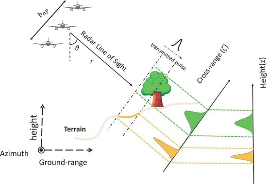
The InSAR model in Equation (10) provides the basis to understand formally the underlying principles of tomographic imaging. Noting that the one term associated with the use of different trajectories is associated with elevation, the integral in Equation (10) can be solved with respect to range and azimuth, yielding:

$$I_{slc}^n(x,r)=e^{\left(-j\frac{4\pi }{\lambda }{r}_n(r;z(x,r))\right)}\int a(x,r,\zeta )e^{(-j{k}_{\zeta }^n·\zeta )}d\zeta$$

(12)

where $a(x,r,\zeta )$ represents the projection of target reflectivity along elevation. A pictorial representation of this projection is given in Figure 2. As highlighted in many papers [1,38,40], this equation can be thought of as the key equation for SAR Tomography. Indeed, the integral in Equation (12) is easily recognized as the Fourier Transform of (the projection of) target reflectivity along elevation, which can therefore be retrieved in a straightforward fashion simple by removing the phase terms outside the integral and by taking the anti-Fourier transform of SLC SAR data at any fixed range/azimuth location. For completeness, we recall that Equation (12) is often expressed by representing the elevation coordinate as a function of height, according to the relationship: $z=\zeta ·sin\left(\theta \right)$, as shown in Figure 2. Up to amplitude terms, this leads to

$$I_{slc}^n(x,r)=e^{\left(-j\frac{4\pi }{\lambda }{r}_n(r;z(x,r))\right)}{\int }_{z_{min}}^{z_{max}}a(x,r,z)e^{(-j{k}_z^n·z)}dz$$

(13)

where integration is performed along the vertical extent of the target and $k_z^n$ is called the phase-to-height conversion factor:

$$k_z^n=\frac{4\pi }{\lambda }\frac{({\theta }_n-\theta )}{sin\theta }$$

(14)

The achievable vertical resolution is also easily derived from standard Fourier theory, and is:

$$\delta z=\frac{2\pi }{max\left(k_z^n\right)}=\frac{\pi }{2}\frac{sin\theta }{max({\theta }_n-\theta )}$$

(15)

3. TomoSAR SAR Processing

3.1. Three-Dimensional TomoSAR Processing

Accurate tomographic focusing can be obtained as a straightforward extension of the backprojection operator expressed in Equation (3) from two to three dimensions. This is achieved by projecting the data onto a set of voxels $(x,y,z)$, and by summing the available data over the 2D aperture spanned by taking all flight times in all trajectories [32]. Mathematically, the 3D back-projection operator is expressed as:

$$T_{3D}(x,y,z)=\sum _n\sum _{\tau }{I}_{rc}^n\left(\tau ,t=\frac{2R(\tau ;x,y,z)}{c}\right)e^{\left(-j\frac{4\pi }{\lambda }R(\tau ;x,y,z)\right)}$$

(16)

where $I_{rc}^n(\tau ,t)$ represents the range compressed data acquired along the n-th trajectory, and $T_{3D}(x,y,z)$ is the focused single-look-complex tomographic cube. In the remainder of this paper, we will refer to the focusing operator in Equation (16) as 3D TomoSAR processing. This approach allows for accurate image formation even for the general case of nonlinear and non-closely spaced trajectories, and guarantees the achievement of the vertical resolution predicted in Equation (15). However, 3D TomoSAR processing is seldom used, as it comes in most cases at the cost of a prohibitive computational burden. As an example: it costs over 10 h for a general CPU processor to focus a 370× 1000 × 180 [m${}^3$] 3D cube (∼${10}^7$ pixels) by the 3D tomographic operator from 15 range-compressed images (1933 azimuth samples and 1894 range bins).

Moreover, implementing tomographic focusing via the operator defined in Equation (16) requires the use of range compressed data, which are usually not made available to users. For this reason, tomographic focusing is quite often carried out based on suitable approximations that lead to simplified focusing operators applied to SLC data, as detailed in the remainder of this section.

3.2. Two-Dimensional TomoSAR

A first important simplification of the focusing operator is obtained by assuming linear and parallel sensor. The assumption of linear trajectories allows to express each SLC image in terms of an integration along iso-range circles, as discussed in the previous section. The further assumption that all trajectories are parallel entails that all iso-range circles belong to a common plane orthogonal to the trajectories at any fixed azimuth location x. As a result, SLC images can be mathematically expressed using Equation (6) as:

$$I_{slc}^n(x,r)=\int \int \int sinc\left(\frac{r-r_n(y^{\prime },z^{\prime })}{\delta r}\right)sinc\left(\frac{x-x^{\prime }}{\delta x}\right)\sigma (x^{\prime },y^{\prime },z^{\prime })e^{(-j\frac{4\pi }{\lambda }{r}_n(y^{\prime },z^{\prime }))d{x}^{\prime }d{y}^{\prime }d{z}^{\prime }}$$

(17)

As the x-coordinate is common to all trajectories, the expression above can be simplified by defining $\beta (x^{\prime },y^{\prime },z^{\prime })=\int sinc\left(\frac{x-x^{\prime }}{\delta x}\right)\sigma (x^{\prime },y^{\prime },z^{\prime })d{x}^{\prime }$, yielding:

$$I_{slc}^n(x,r)=\int sinc\left(\frac{r-r_n(y^{\prime },z^{\prime })}{\delta r}\right)\beta (x,y^{\prime },z^{\prime })e^{\left(-j\frac{4\pi }{\lambda }{r}_n(y^{\prime },z^{\prime })\right)}d{y}^{\prime }d{z}^{\prime }$$

(18)

This equation states a direct relation between target reflectivity at a fixed azimuth location x and the ensemble of SLC images at the same azimuth location. By virtue of this relation, tomographic focusing can be obtained directly from SLC images via a 2D back-projection operator for any fixed azimuth location x:

$$T_{2D}(x,y,z)=\sum _n{I}_{slc}^n\left(x,r=r_n(y^{\prime },z^{\prime })\right)e^{\left(j\frac{4\pi }{\lambda }{r}_n(y^{\prime },z^{\prime })\right)}$$

(19)

which we will refer to as 2D Tomographic processing.

Obviously, the validity of this approach becomes questionable in the case of loosely controlled trajectories, which results in iso-range circles to be tilted depending on trajectory heading, thus occupying an extended interval of azimuth positions (see Figure 3). In this case, SLC images need to be properly projected onto a common reference grid assuming a reference surface topography, either by co-registration or back-projection, see Equation (3). Yet, targets that do not belong to the reference surface will appear in SLC images at different azimuth locations, depending on target height with respect to the reference surface and trajectory heading, thus invalidating the 2D Tomographic processing approach. The limit of applicability of this approach can be discussed in quantitative terms by expressing the azimuth shift with height as a function of trajectory heading:

$$\Delta x\simeq -\left(\frac{tan\alpha }{tan\theta }+tan\beta \right)\Delta h$$

(20)

where $\alpha$ and $\beta$ are the tilts with yaw and pitch angles as defined in Figure 3, and $\Delta h$ is target height with respect to the reference surface.

Equation (20) states the arising of an azimuth migration problem affecting in case of nonparallel trajectories: azimuth migration grows with target height and is scaled according to trajectory direction. As azimuth migration becomes comparable with azimuth resolution, the operator in Equation (19) starts mixing contributions from different targets, leading to poor focusing performance. A precise condition for the applicability of 2D SAR Processing can be cast by requiring azimuth migration not to exceed half a resolution cell, leading to:

$$|\Delta h|<\frac{\delta x}{2}\frac{tan\theta }{tan\alpha +tan\beta tan\theta }$$

(21)

3.3. One-Dimensional TomoSAR

One-Dimensional approaches to tomographic processing, which we refer to as 1D TomoSAR processing, are those based on the InSAR model discussed in Section 2.1 that lead to Equation (12), here reported for the sake of clarity:

$$I_{slc}^n(x,r)=e^{\left(-j\frac{4\pi }{\lambda }{r}_n\left(r;z(x,r)\right)\right)}{\int }_{z_{min}}^{z_{max}}a(x,r,z)e^{(-j{k}_z^{n}z)}dz$$

(22)

Among the most popular algorithms for inverting Equation (22) is Beamforming [41], which consists of taking the inverse Fourier transform of phase compensated SLC data:

$$T_{BF}(x,r,z)=\sum _n{I}_{slc\_comp}^n(x,r)e^{\left(j{k}_z^{n}z\right)}$$

(23)

with $I_{slc\_comp}^n=I_{slc}^n(x,r)e^{\left(j\frac{4\pi }{\lambda }{r}_n\left(r;z(x,r)\right)\right)}$.

As discussed in many papers, tomographic imaging by Beamforming suffers from limitations concerning vertical resolution, which is strictly ruled by Equation (15), and presence of side-lobes in the case that the distribution of incidence angles ${\theta }_n$ is not uniform [29]. For this reason, a number of algorithms from spectral analysis have been proposed and successfully demonstrated in the literature, such as Capon filtering [29], MUSIC [29], compressive sensing [27,28], subspace fitting [31], and wavelet-based representation [30]. Still, it is important to bear in mind that all those algorithms are strictly based on the assumptions within the InSAR model in Section 2.1; namely, trajectories have to be not only parallel, to within the conditions discussed earlier before this section, but also sufficiently closely spaced, as we discuss hereinafter.

For parallel trajectories, all iso-range circles passing through a specific range/azimuth location are entirely confined within a single plane, which, for the sake of simplicity, we assume here to be the $(y,z)$ plane, as depicted in Figure 4. In this example, two targets $P_1$ and $P_2$ are found at the same distance from the Master track, and thus both belong to the iso-range circle relative to the Master track (in black dash). The same two points are found at different distances from the Slave track, which differ by

$$\Delta r\simeq \frac{{\theta }_n-\theta }{sin\theta }\Delta h$$

(24)

where $\Delta h$ is the height difference between the two targets, and $\Delta r$ represents the residual range migration of target $P_2$ relative to target $P_1$. Equation (24) simply implies that the InSAR model is only valid as long as residual migration is lower than the range resolution. In analogy with the previous section, we cast a condition for the applicability of 1D TomoSAR processing by requiring residual range migration not to exceed half a resolution cell, leading to:

$$|\Delta h|<\frac{\delta r}{2}\frac{sin\theta }{{\theta }_n-\theta }$$

(25)

where $\Delta h$ represents the maximum vertical extent for the scene for which 1D TomoSAR processing can be applied.

In summary, the main features of the discussed approaches to tomographic focusing are recapped in

Table 1. Summary of the discussed approaches to TomoSAR processing.

Approaches	1D TomoSAR	2D TomoSAR	3D TomoSAR
Required Data	Focused SLC data;	Focused SLC data;	Raw data (range compressed);
Inversion strategy	Baseline to height for each fixed range/ azimuth location	Range/baseline to ground range/height for each fixed azimuth location	Fast time/slow time/ baseline to azimuth/ ground range/height
Underlying assumptions	Parallel and closely spaced trajectories	Parallel trajectories	-
Conditions for validity	Azimuth migration (20) and Range migration (24)	Azimuth migration (20)	-
Notes	Low computational burden; Possibility to re-use well known algorithms from spectral analysis	Moderately low computational burden	Very high computational burden

.

4. 3D TomoSAR by Sub-Sampled Defocusing/Refocusing

The aim of this section is to illustrate an operational algorithm designed for implementing 3D TomoSAR processing based on SLC data at a computational burden affordable to standard computers.

4.1. Algorithm Rational

The algorithm is articulated in two main steps, as pictorially depicted in Figure 5. The first step consists in the generation of range-compressed raw data by defocusing the available SLC data. This step is implemented by projecting SLC data onto flight trajectories, formally:

$$I_{rc}^n(\tau ,t)=\int \int sinc\left(B\left(t-\frac{2R_n\left(\tau ;x,y,z(x,y)\right)}{c}\right)\right)e^{\left(-\frac{4\pi }{\lambda }{R}_n\left(\tau ;x,y,z(x,y)\right)\right)}{I}_{slc}^n(x,y)dxdy$$

(26)

where $R_n\left(\tau ;x,y,z(x,y)\right)$ is the distance from a point at $\left(x,y,z(x,y)\right)$ to the position of the nth sensor at time $\tau$, and $z(x,y)$ is the reference surface used for focusing SLC data. Importantly, we note that Equation (26) has to be implemented by using the same flight trajectories and reference topography surfaces that were used in the focusing processor that generated SLC data. Accordingly, this information should always be provided along with SLC data. The second step consists in the generation of 3D tomographic cubes, or voxels, by time domain back-projection, implemented as indicated in Equation (16). Note that step 2 can be implemented by using different trajectories than those used at step. This is required when more accurate navigational data are available than those used for producing individual SLC images, as it is the typical case where flight trajectories have been refined through interferometric analysis, see for example [38].

The strategy to implement both steps at an acceptable computational cost is based on the consideration that a single tomographic voxel is not contributed by all pixels within SLC images, but only by those pixels within a local neighbor of the voxel position, in which the spatial extent is obtained by calculating range and azimuth migration, as discussed in previous sections. This property of locality is exploited to compute individual tomographic by defocusing only a small portion of SLC images. In doing so, we achieve two-fold beneficial effects on releasing the computational burden. In the first place, the interval of integration in Equation (26) is largely reduced, lowering the cost per generated sample. In addition, defocusing a small neighbor of adjacent pixels results in a much narrower instantaneous Doppler bandwidth as compared to defocusing the entire scene, which determines a strong correlation across different slow time ($\tau$) samples in the raw data. Such a correlation is exploited to generate strongly sub-sampled raw data, hence dramatically reducing the number of samples both in the generation of raw data in Equation (26) and in the back-projection summation in Equation (16), with obvious advantages in terms of memory allocation and cost per generated voxel.

Based on these principles, the algorithm is designed to scan the scene by sequentially producing high-resolution tomographic sections in the ground range/height $(y,z)$ plane for a conveniently small azimuth (x) interval. The overall algorithm is summarized in the Algorithm 1. Implementation details are discussed in the next subsections.

Algorithm 1 Sub-sampled defocusing and refocusing.

Input: The set of SLC images, $I_{slc}^n$; 1: Reference DEM, $z^n(x,y)$; Original trajectory information, $S_{orig}^n$; Refined trajectory information, $S_c^n$; Output: Focused 3D cube, $T_{3D}$; 2: Fix the maximum height interval $\Delta h$ with respect to the reference surface assumed; 3: for a fixed azimuth interval, $x-x_{max},x+x_{max}$ do 4:     Evaluate maximum azimuth migration, $\Delta x$, from $S_c^n$ using Equation (20). 5:     Fix raw data sampling time as described in Section 4.2, accounting for a total azimuth extent $x_e=2(x_{max}+\Delta x)$. 6:     Defocus all SLC data in the interval $(x-x_e/2,x+x_e/2)$ using the projection operator in Equation (26). An efficient implementation of this step is described in Section 4.3. 7:     Refocus the data in the $(y,z)$ plane in the azimuth interval $x-x_{max},x+x_{max}$ using the 3D back-projection operator in Equation (16). An efficient implementation of this step is described in Section 4.3; 8: end for 9: return$T_{3D}$;

4.2. Raw Data Sub-Sampling

Considering a small neighborhood of adjacent targets, the raw data decorrelation time can be lower-bounded by considering the inverse of the instantaneous Doppler bandwidth along the aperture:

$${\tau }_{dec}\ge \frac{1}{max\left(B_d\left(\tau \right)\right)}$$

(27)

An expression for $B_d$ is easily found by considering the instantaneous Doppler frequency associated with a single target at $(x,y,z)$:

$$f_d=\frac{2}{\lambda }\frac{dR(\tau ;x,y,z)}{d\tau }$$

(28)

Accordingly, the instantaneous Doppler bandwidth resulting from a small neighborhood of targets is obtained as:

$$B_d\left(\tau \right)=ma{x}_{xyz}\left(f_d\right)-mi{n}_{xyz}\left(f_d\right)$$

(29)

The role of the considered neighborhood can be made explicit by considering the simplified case of a linear trajectory, in which case:

$$f_d\simeq \frac{2v_s}{\lambda }sin\left(\psi \right)$$

(30)

with $\psi$ the local squint angle and $v_s$ platform velocity. The maximum Doppler bandwidth along the aperture is then estimated as:

$$B_d\left(\tau \right)=\frac{2v_s}{\lambda r}\Delta x_e$$

(31)

with r the closest approach distance of the center of the considered neighborhood and $2x_e$ its total azimuth extent. In this case, it follows that raw data can be generated at a sampling interval up to:

$$\Delta \tau \le \frac{\lambda }{2v_s{x}_e}min\left(r\right)$$

(32)

which sets the maximum Pulse Repetition Interval (PRI) for the correct generation of raw data. It is worth noting in case of no azimuth migration ($\Delta x=0$), the generation of a tomographic section at a single azimuth position ($x_{max}=0$) corresponds to generating just one single slow time. In this particular case, the algorithm here discusses defaults automatically to 2D TomoSAR processing.

4.3. Detailed Implementation

The computational costs associated with the projection and back-projection operators in Equations (26) and (16) can be largely lowered by expressing both operators in terms of operations that are usually available as fast built-in functions in most programming languages.

For the case of back-projection, it is immediate to note that the term $I_{rc}^n\left(\tau ,t=\frac{2R(\tau ;x,y,z)}{c}\right)$ in the inner summation of Equation (16) can be obtained by interpolating the raw data at fast-time instants $t=\frac{2R(\tau ;x,y,z)}{c}$. This operation can be performed quite efficiently by using simple interpolation kernels, like linear or even nearest-neighbor interpolation, ensuring accurate results by using over-sampled data in the fast time domain. In our implementation, we typically use an oversampling factor of four with respect to the inverse pulse bandwidth.

The same principle can be applied to the projection operator by noting that Equation (26) can be recast in the form of convolution as:

$$I_{rc}^n(\tau ,t)=sinc\left(Bt\right)*A\left(t\right)$$

(33)

where

$$A\left(t\right)=\int \delta \left(t-\frac{2R_n\left(\tau ;x,y,z(x,y)\right)}{c}\right)I_{rot}^n(x,y)dxdy$$

(34)

and

$$I_{rot}^n(x,y)=e^{\left(-j\frac{4\pi }{\lambda }{R}_n\left(\tau ;x,y,z(x,y)\right)\right)}{I}_{slc}^n(x,y)$$

(35)

The time signal $A\left(t\right)$ represents the sum of all phase-rotated pixels, $I_{rot}^n$, that are found at distance $R=\frac{ct}{2}$ from the sensor at slow time instant $\tau$. This signal can be computed by range binning, that is by rearranging phase-rotated pixels within range bins according to their distance from the sensor, and by accumulating all pixels values falling in the same range bin. The accuracy of the result is ensured by properly choosing the bin size, $\Delta R$, which determines the oversampling factor of the signal $A\left(t\right)$ according to: $\Delta t=\frac{2}{c}\Delta R$. As in the case of back-projection, we use an oversampling factor of four with respect to the inverse of pulse bandwidth.

4.4. GPU-Based Implementation

The defocusing and refocusing operations described above are well suited for parallel implementations on GPUs, if available. In this study, the NVIDIA Compute Unified Architecture (CUDA) [42] is assumed as framework.

The defocusing and refocusing algorithms can be seen as massively parallel problems. Specifically, for the projection operator, the phase rotation operation in Equation (35) can be executed for each SLC pixel independently. The thread, which is the fundamental processing unit in CUDA, takes the responsibility of the calculation task of each SLC pixel. After that, the accumulation over pixels in Equation (34) requires special care, since the signals from different SLC pixels with similar distances will be collected into the same range bin. This kind of accumulation has to use atomic operations in CUDA, in order to avoid access conflict in parallel processing [43]. At last, the FFT-based convolution is easily implemented with the aid of the CUFFT library (a highly optimized GPU FFT library in CUDA). As for the refocusing, coherent accumulation in Equation (16) is parallelly implemented by invoking the GPU kernel to estimate the phase rotated signals at each slow time $\tau$ and setting one outer loop to accumulate the signals over $\tau$. This kind of implementation can fully exploit the high GPU memory bandwidth.

Optimized GPU implementation of the projection and back-projection operators are presented in Figure 6 and Figure 7. Some CUDA optimization tricks (see [44]) are also used to enhance the processing efficiency for each GPU-based kernel.

5. Numerical Simulations

The simulated data were used to give a stepwise analysis of the advantages and limitations of 1D, 2D, and 3D TomoSAR approaches. Two kinds of simulated experiments are carried out to evaluate the tomographic performance of each method regarding the sensor trajectory stability, spatial resolutions, and target thickness. The first test assumed parallel trajectories and explored the tomographic performance differences between 1D and 2D TomoSAR processing with respect to low and high resolution configurations. The second test intended to compare each approach under high resolution systems with nonparallel trajectories. The relevant simulated parameters are summarized in

Table 2. Relevant simulation parameters.

Simulation Parameters
Carrier Frequency	500 [MHz] (P band)
Bandwidth	100 or 150 [MHz]
Number of Acquisitions	21
Vertical Baseline	100 [m]
Height of target Layers	0, 20, and 40 [m]
Height of Ambiguity	∼70 [m]

. The simulated scene includes distributed targets drawn from a circular normal complex distribution, and consists of three horizontal layers at 0, 20, and 40 m above a flat topography, which is assumed as the reference surface for the generation of SLC data.

In the first test, raw data were simulated under parallel sensor trajectories with 100 and 150 MHz bandwidths, respectively. One-dimension TomoSAR approaches retrieved the tomographic profiles from SAR data in both bandwidth configurations. In contrast, 2D TomoSAR methods only reconstruct the higher resolution tomographic profiles (see Figure 8).

Results from the first test (parallel trajectories) are shown in Figure 8. The panel in the first two rows were obtained by 1D TomoSAR processing, assuming a bandwidth 100 and 150 MHz. It is immediate to see that the surface at 0 m is correctly focused in all cases. This is because the 0 m surface has been taken as the reference in the generation of SLC data, hence all SLC are perfectly co-registered at this surface. This is not the case that surfaces at 20 m and 40 m, for which residual range migration leads to defocusing. As expected, the impact on 1D TomoSAR processing is more severe in the case of 150 MHz data, for which range migration is larger as compared to range resolution, leading to power losses of around 5 dB at the 40 m surface.

In the second test, the raw data were generated assuming a 150 MHz bandwidth and nonparallel trajectories. Trajectories were simulated assuming using different combinations of yaw and pitch angles, drawn from a random normal distribution with a standard deviation of 1.5 deg. Results are shown in Figure 9, where the top, middle, and bottom rows refer to the cases of 1D, 2D, and 3D TomoSAR processing. In this case, the presence of residual range and azimuth migration leads to strong defocusing when using 1D and 2D TomoSAR processing, resulting in power losses of 10 dB at the 40 m surface.

To gain more insights, we plot in Figure 10 the percentage of valid image pairs as a function of the vertical extent of the scene. An image pair is defined “valid” if range and azimuth residual migration are less than half a resolution cell, that is if the conditions cast in Equations (20) and (24) hold. In the considered example, the percentage of valid pairs is $28\%$ at 20 m and $10\%$ at 40 m, which causes severe defocusing for height locations far from the reference surface. The use of 2D TomoSAR partly improves the percentage of valid pairs to $45\%$ at 20 m and $25\%$ at 40 m by compensating for residual range migration. Still, imaging quality cannot be fully recovered, as residual azimuth migration remains uncompensated.

6. Experiments on AlpTomoSAR Data

The ESA campaign AlpTomoSAR was flown by MetaSensing in 2014 at the Mittelbergferner glacier, in the Austrian study [23], with the aim of demonstrating the use of SAR tomography for studying the internal structure of glaciers. SAR data were acquired at a central frequency of 1275 MHz, with a pulse bandwidth of 150 MHz. The sensor was flown along roughly 1300 m above the surface along an oval race-track configuration, to provide two independent data-sets from two opposite views. The flight lines were designed to have 10 parallel, closely spaced tracks plus other more largely spaced tracks to improve resolution. Flight trajectories have been perturbed by turbulent phenomena in proximity of the peaks, resulting in a dispersion of about 13 and 1m rms in the horizontal and vertical direction, respectively. In both views, the total baseline aperture resulted in a vertical resolution of approximately 2 m in free-space. SLC data have been focused through time domain back-projection onto a reference surface derived from a Lidar survey acquired in 2010.

Flight trajectories and the reference surface are included in the final data delivery along with SLC data. AlpTomoSAR data were processed in [38] using the Phase Center Double Localization algorithm to produce accurate information about flight trajectories, since the accuracy of original navigational data was found not to be sufficient for tomographic imaging. In this study, tomographic focusing is carried out using the same trajectories produced in [38].

Residual range and azimuth migrations are analyzed in Figure 11. For both views, it is observed that residual azimuth migrations are the main factor that limits the number of valid pairs in 1D and 2D TomoSAR processing, which gets as low as $10\%$ at 50 m from the reference surface. As shown in [23], AlpTomoSAR data provide sensitivity to the whole ice body, including the ice surface and the bedrock at approximately 60 m below. This value has to be scaled for the ice refractivity index (about 1.8), yielding an equivalent vertical extent over 100 m in free-space. Accordingly, a height offset of at least 50 m with respect to the reference surface has to be accounted for, even considering the best case where all SLC data are co-registered in the middle of the glacier vertical extent.

Tomographic vertical sections generated using 1D, 2D, and 3D TomoSAR processing are displayed in Figure 12. For each panel, the overlaid red line indicates ice surface topography from the Lidar DTM. Similar to the case of numerical simulations, by comparing the three panels, it is immediate to see that only using 3D TomoSAR processing, it is possible to image subsurface layers. One-dimension TomoSAR processing is clearly seriously affected by both azimuth and range migration, so that only small neighborhood about the reference surface can be recovered. Two-dimension TomoSAR processing is only partly capable of detecting the presence of internal structures, but imaging quality is strongly degraded as a result of uncompensated residual azimuth migration.

Sub-Sampled Defocusing/Refocusing: Imaging Quality and Efficiency

In this section, we analyze the quality of 3D Tomographic processing as implemented using different sub-sampling factors. Considering all passes, the maximum residual azimuth migration turned out to be $\Delta x$ = 15 m at a height of 100 m from the reference topography, which sets the extent of the azimuth extent to be defocused for generating a vertical section at any single azimuth location ($x_{max}$ = 0 m). Following the discussion in Section 4.2, such a value corresponds to a maximum PRI of approximately $\Delta {\tau }_{max}=5.4$ s, where we conventionally assumed to simulate platform motion at 1 m/s (platform velocity being irrelevant since temporal decorrelation is not considered).

To provide a term of reference against which to evaluate imaging quality and computational time, tomographic processing is also implemented through a processing approach hereafter referred to as Global Algorithm, which consists of defocusing SLC data over a large azimuth interval at once, and by subsequently generating tomographic section at all azimuth locations. In this case, raw data are generated by sampling the synthetic aperture at a spatial interval of two wavelengths (0.47 m), which corresponds to approximately half the azimuth resolution of SLC data. Assuming a platform velocity of 1 m/s, the resulting PRI is approximately $\Delta {\tau }_{min}=0.47$ s. Accordingly, the sub-sampled algorithm allows for a maximum PRI relaxation factor up to 11 with respect to the global algorithm.

Imaging quality is addressed in Figure 13, which displays the vertical sections obtained by the global algorithm (first panel from top), and by the sub-sampled one, assuming a PRI relaxation factor of 4, 8, 16 (second to last panels from top). Consistently with our analysis in Section 4, we observe no degradation with respect to the tomographic section produced by the global algorithm in the top panel as long as the relaxation factor is lower than 11, that is when raw data are generated at a PRI faster than 5.4 s.

Table 3. The CPU computational times of global algorithm and local algorithms.

Algorithm [PRI Relaxation Factor]	Runtime	Speed-up Factor
Global algorithm [1x]	9.71h	1x
Sub-sampled/ $x_{max}$ = 0 m [4x]	3.6 h	2.7x
Sub-sampled/ $x_{max}$ = 0 m [8x]	1.7 h	5.6x
Sub-sampled/ $x_{max}$ = 7.5 m [4x]	1.8 h	5.4x
Sub-sampled/ $x_{max}$ = 7.5 m [7x]	1 h	9.5x

reports the total computational times required for the generation of a tomographic cube of size: 300 m in azimuth, 1000 m in ground range, 180 m in height. Three algorithms are compared; namely, the global algorithm (first row), the sub-sampled algorithm as implemented by subsequently focusing single azimuth lines ($x_{max}$ = 0 m), and the sub-sampled algorithms as implemented by subsequently focusing intervals of 15 m in azimuth ($x_{max}$ = 7.5 m), resulting in a maximum PRI relaxation factor equal to seven.

Here, it is easy to see that the use of the sub-sampled algorithm provides a substantial benefit, resulting in a net improvement of up to 9.5 with respect to the global algorithm.

Total computational times required by the GPU implementation are shown in

Table 4. The GPU computational times of the global algorithm (without PRI relaxation) and local algorithms (with different PRI relaxation factors).

Algorithm [PRI Relaxation Factor]	Runtime	Speed-up Factor
Global algorithm [1x]	18.4 s	1x
Sub-sampled/ $x_{max}$ = 7.5 m [4x]	8.7 s	2.1x
Sub-sampled/ $x_{max}$ = 7.5 m [7x]	6.8 s	2.7x

, where we compare the global algorithm against the sub-sampled algorithm as implemented by subsequently focusing intervals of 15 m in azimuth.

The experiments were carried out on a platform with an Intel(R) Core i7-8700K CPU and an Nvidia Titan V GPU.

Table 5. GPU Specifications.

	GTX Titan V
Architecture	GV100
Number of cores	5120
Dedicated Memory	12 GB
Clock rate	1455 MHz
Driver mode	Tesla Compute Cluster

shows the specifications of the GPUs used in our experiments. The driver mode of GPUs was all set as Tesla Compute Cluster (TCC) mode for a better performance. The source code was compiled with -O2 optimization under the Microsoft Visual Studio 2017 and CUDA Toolkit 10.2.

The GPU implementation entails a dramatic improvement, allowing the generation of a large tomographic cube in few seconds. Also in this case, though, use of the sub-sampled algorithm allows a significant cost reduction with respect to the global one. Finally, it is worth noting that the global algorithm could not be used to generate tomographic cubes with an azimuth extent larger than 2000 m, due to saturation of on-board memory. This problem does not affect the sub-sampled algorithm, for which memory occupation only depends on the extent of the azimuth interval to be defocused.

Furthermore,

Table 6. The CPU computational times of the 1D, and 2D TomoSAR processing.

Processing Approach	1D TomoSAR	2D TomoSAR
Runtime	14.51 s	23.90 s

shows the processing time required by 1D, 2D tomographic approaches on CPU. It follows that both approaches have such low computational burdens that only tens of seconds are needed to generate the 3D cube from SLC images. It also indicates that our proposed 3D full processing implementation has effectively reduced the computational time into the same level as the simplified tomographic algorithms.

7. Conclusions

This paper was intended to shed light on which processing strategies are suitable for the correct generation of high-resolution and accurate tomographic products. We have shown that the popular vector-to-vector 1D processing approach, largely assumed in the literature and declared in many different forms using spectral estimation techniques, is only applicable for cases where residual range migration does not exceed range resolution, that is the case where data are characterized by coarse vertical resolution. Accurate processing of high-resolution tomographic data can be carried out by assuming a 2D processing approach, where bi-dimensional back-projection is carried out at each azimuth location. Still, this approach can only be applied in the case of approximately parallel trajectories, for which residual azimuth migration does not exceed azimuth resolution. The assumption of parallel trajectories is, in general, well-justified whenever data acquisition is carried out using very stable aircrafts under non-turbulent conditions. This is, however, not always the case, as the AlpTomoSAR campaign demonstrates. For such cases, tomographic processing should then be implemented by focusing the raw data in the three-dimensional space by 3D back-projection. This processing option clearly has two important drawbacks, represented by the enormous demands in terms of computational costs (processing time and memory allocation) and the need to access raw data, which are usually not provided as part of standard data delivery. Both these topics were addressed in the second part of this paper, where we proposed a processing algorithm based on sub-sampled defocusing and refocusing, consisting of the generation of sub-sampled raw data from available SLC data, to be focused afterward in the three-dimensional space at a largely reduced computational cost. The proposed algorithm was applied to process data from AlpTomoSAR, and demonstrated to produce accurate results, with hardly distinguishable differences with respect to reference data produced without applying any sub-sampled factor. Finally, the proposed algorithm is also easily implemented using GPU processing, which grants a dramatic reduction in computational time. Accordingly, we deem the present work fully demonstrates that the quality of a tomographic airborne survey is not limited in any sense by platform stability during the acquisition, clearly as long as tomographic processing is correctly implemented by correctly accounting for the sensor trajectories. With regard to the last point, we remark the importance that any information used to produce SLC data is made available to final users, including, in particular, sensor trajectories and the reference surface elevation map used for focusing or co-registering SLC data.

References

1. Reigber, A.; Moreira, A. First demonstration of airborne SAR tomography using multibaseline L-band data. IEEE Trans. Geosci. Remote. Sens. 2000, 38, 2142–2152. [Google Scholar] [CrossRef]
2. Curlander, J.C.; McDonough, R.N. Synthetic Aperture Radar; Wiley: New York, NY, USA, 1991; Volume 11. [Google Scholar]
3. Tebaldini, S. Algebraic synthesis of forest scenarios from multibaseline PolInSAR data. IEEE Trans. Geosci. Remote Sens. 2009, 47, 4132–4142. [Google Scholar] [CrossRef]
4. Tebaldini, S.; Rocca, F. Multibaseline Polarimetric SAR Tomography of a Boreal Forest at P- and L-Bands. IEEE Trans. Geosci. Remote Sens. 2012, 50, 232–246. [Google Scholar] [CrossRef]
5. Mariotti d’Alessandro, M.; Tebaldini, S. Phenomenology of P-Band Scattering From a Tropical Forest Through Three-Dimensional SAR Tomography. IEEE Geosci. Remote. Sens. Lett. 2012, 9, 442–446. [Google Scholar] [CrossRef]
6. d’Alessandro, M.M.; Tebaldini, S.; Rocca, F. Phenomenology of ground scattering in a tropical forest through polarimetric synthetic aperture radar tomography. IEEE Trans. Geosci. Remote. Sens. 2013, 51, 4430–4437. [Google Scholar] [CrossRef]
7. Minh, D.H.T.; Le Toan, T.; Rocca, F.; Tebaldini, S.; Villard, L.; Réjou-Méchain, M.; Phillips, O.L.; Feldpausch, T.R.; Dubois-Fernandez, P.; Scipal, K.; et al. SAR tomography for the retrieval of forest biomass and height: Cross-validation at two tropical forest sites in French Guiana. Remote. Sens. Environ. 2016, 175, 138–147. [Google Scholar] [CrossRef] [Green Version]
8. Frey, O.; Meier, E. Analyzing tomographic SAR data of a forest with respect to frequency, polarization, and focusing technique. IEEE Trans. Geosci. Remote Sens. 2011, 49, 3648–3659. [Google Scholar] [CrossRef] [Green Version]
9. Yang, X.; Tebaldini, S.; Mariotti d’Alessandro, M.; Liao, M. Tropical Forest Height Retrieval Based on P-Band Multibaseline SAR Data. IEEE Geosci. Remote. Sens. Lett. 2019, 1–5. [Google Scholar] [CrossRef]
10. Tello, M.; Cazcarra-Bes, V.; Pardini, M.; Papathanassiou, K. Forest Structure Characterization From SAR Tomography at L-Band. IEEE J. Sel. Top. Appl. Earth Obs. Remote. Sens. 2018, 11, 3402–3414. [Google Scholar] [CrossRef] [Green Version]
11. Cazcarra-Bes, V.; Tello-Alonso, M.; Fischer, R.; Heym, M.; Papathanassiou, K. Monitoring of Forest Structure Dynamics by Means of L-Band SAR Tomography. Remote. Sens. 2017, 9, 1229. [Google Scholar] [CrossRef] [Green Version]
12. Pardini, M.; Tello, M.; Cazcarra-Bes, V.; Papathanassiou, K.P.; Hajnsek, I. L- and P-Band 3-D SAR Reflectivity Profiles Versus Lidar Waveforms: The AfriSAR Case. IEEE J. Sel. Top. Appl. Earth Obs. Remote. Sens. 2018, 11, 3386–3401. [Google Scholar] [CrossRef]
13. Neumann, M.; Ferro-Famil, L.; Reigber, A. Estimation of forest structure, ground, and canopy layer characteristics from multibaseline polarimetric interferometric SAR data. IEEE Trans. Geosci. Remote Sens. 2009, 48, 1086–1104. [Google Scholar] [CrossRef] [Green Version]
14. Lavalle, M.; Hensley, S. Extraction of structural and dynamic properties of forests from polarimetric-interferometric SAR data affected by temporal decorrelation. IEEE Trans. Geosci. Remote Sens. 2015, 53, 4752–4767. [Google Scholar] [CrossRef]
15. Blomberg, E.; Ferro-Famil, L.; Soja, M.J.; Ulander, L.M.; Tebaldini, S. Forest biomass retrieval from l-band sar using tomographic ground backscatter removal. IEEE Geosci. Remote. Sens. Lett. 2018, 15, 1030–1034. [Google Scholar] [CrossRef]
16. Ulander, L.M.; Monteith, A.R.; Soja, M.J.; Eriksson, L.E. Multiport vector network analyzer radar for tomographic forest scattering measurements. IEEE Geosci. Remote. Sens. Lett. 2018, 15, 1897–1901. [Google Scholar] [CrossRef]
17. Rekioua, B.; Davy, M.; Ferro-Famil, L.; Tebaldini, S. Snowpack permittivity profile retrieval from tomographic SAR data. Comptes Rendus Phys. 2017, 18, 57–65. [Google Scholar] [CrossRef]
18. Ferro-Famil, L.; Leconte, C.; Boutet, F.; Phan, X.; Gay, M.; Durand, Y. PoSAR: A VHR tomographic GB-SAR system application to snow cover 3-D imaging at X and Ku bands. In Proceedings of the 2012 9th European Radar Conference, Amsterdam, The Netherlands, 31 October–2 November 2012; pp. 130–133. [Google Scholar]
19. Frey, O.; Werner, C.L.; Caduff, R.; Wiesmann, A. A time series of SAR tomographic profiles of a snowpack. In Proceedings of the EUSAR 2016: 11th European Conference on Synthetic Aperture Radar, Hamburg, Germany, 6–9 June 2016; pp. 1–5. [Google Scholar]
20. Leinss, S.; Parrella, G.; Hajnsek, I. Snow height determination by polarimetric phase differences in X-band SAR data. IEEE J. Sel. Top. Appl. Earth Obs. Remote. Sens. 2014, 7, 3794–3810. [Google Scholar] [CrossRef] [Green Version]
21. Banda, F.; Dall, J.; Tebaldini, S. Single and multipolarimetric P-band SAR tomography of subsurface ice structure. IEEE Trans. Geosci. Remote Sens. 2015, 54, 2832–2845. [Google Scholar] [CrossRef]
22. Wu, X.; Jezek, K.C.; Rodriguez, E.; Gogineni, S.; Rodriguez-Morales, F.; Freeman, A. Ice Sheet Bed Mapping With Airborne SAR Tomography. IEEE Trans. Geosci. Remote Sens. 2011, 49, 3791–3802. [Google Scholar] [CrossRef]
23. Tebaldini, S.; Nagler, T.; Rott, H.; Heilig, A. Imaging the Internal Structure of an Alpine Glacier via L-Band Airborne SAR Tomography. IEEE Trans. Geosci. Remote Sens. 2016, 54, 7197–7209. [Google Scholar] [CrossRef]
24. Yitayew, T.G.; Ferro-Famil, L.; Eltoft, T.; Tebaldini, S. Lake and fjord ice imaging using a multifrequency ground-based tomographic SAR system. IEEE J. Sel. Top. Appl. Earth Obs. Remote. Sens. 2017, 10, 4457–4468. [Google Scholar] [CrossRef]
25. Ponce, O.; Prats, P.; Scheiber, R.; Reigber, A.; Hajnsek, I.; Moreira, A. Polarimetric 3-D imaging with airborne holographic SAR tomography over glaciers. In Proceedings of the 2015 IEEE International Geoscience and Remote Sensing Symposium (IGARSS), Milan, Italy, 26–31 July 2015; pp. 5280–5283. [Google Scholar]
26. Fischer, G.; Jäger, M.; Papathanassiou, K.P.; Hajnsek, I. Modeling the Vertical Backscattering Distribution in the Percolation Zone of the Greenland Ice Sheet With SAR Tomography. IEEE J. Sel. Top. Appl. Earth Obs. Remote. Sens. 2019, 12, 4389–4405. [Google Scholar] [CrossRef]
27. Zhu, X.X.; Bamler, R. Tomographic SAR Inversion by L1 -Norm Regularization—The Compressive Sensing Approach. IEEE Trans. Geosci. Remote Sens. 2010, 48, 3839–3846. [Google Scholar] [CrossRef] [Green Version]
28. Budillon, A.; Evangelista, A.; Schirinzi, G. Three-Dimensional SAR Focusing From Multipass Signals Using Compressive Sampling. IEEE Trans. Geosci. Remote Sens. 2011, 49, 488–499. [Google Scholar] [CrossRef]
29. Gini, F.; Lombardini, F. Multibaseline cross-track SAR interferometry: A signal processing perspective. IEEE Aerosp. Electron. Syst. Mag. 2005, 20, 71–93. [Google Scholar] [CrossRef]
30. Aguilera, E.; Nannini, M.; Reigber, A. Wavelet-Based Compressed Sensing for SAR Tomography of Forested Areas. IEEE Trans. Geosci. Remote Sens. 2013, 51, 5283–5295. [Google Scholar] [CrossRef] [Green Version]
31. Huang, Y.; Levy-Vehel, J.; Ferro-Famil, L.; Reigber, A. Three-Dimensional Imaging of Objects Concealed Below a Forest Canopy Using SAR Tomography at L-Band and Wavelet-Based Sparse Estimation. IEEE Geosci. Remote. Sens. Lett. 2017, 14, 1454–1458. [Google Scholar] [CrossRef]
32. Frey, O.; Morsdorf, F.; Meier, E. Tomographic imaging of a forested area by airborne multi-baseline P-band SAR. Sensors 2008, 8, 5884–5896. [Google Scholar] [CrossRef]
33. Ponce, O.; Prats-Iraola, P.; Pinheiro, M.; Rodriguez-Cassola, M.; Scheiber, R.; Reigber, A.; Moreira, A. Fully Polarimetric High-Resolution 3-D Imaging With Circular SAR at L-Band. IEEE Trans. Geosci. Remote Sens. 2014, 52, 3074–3090. [Google Scholar] [CrossRef]
34. Ponce, O.; Prats-Iraola, P.; Scheiber, R.; Reigber, A.; Moreira, A. First Airborne Demonstration of Holographic SAR Tomography With Fully Polarimetric Multicircular Acquisitions at L-Band. IEEE Trans. Geosci. Remote Sens. 2016, 54, 6170–6196. [Google Scholar] [CrossRef]
35. Frey, O.; Magnard, C.; Ruegg, M.; Meier, E. Focusing of Airborne Synthetic Aperture Radar Data From Highly Nonlinear Flight Tracks. IEEE Trans. Geosci. Remote Sens. 2009, 47, 1844–1858. [Google Scholar] [CrossRef] [Green Version]
36. Torgrimsson, J.; Dammert, P.; Hellsten, H.; Ulander, L.M.H. SAR Processing Without a Motion Measurement System. IEEE Trans. Geosci. Remote Sens. 2019, 57, 1025–1039. [Google Scholar] [CrossRef]
37. Cumming, I.G.; Dettwiler, M.; Wong, F.H. Digital signal Processing of Synthetic Aperture Radar Data: Algorithms and Implementation; ArtechHouse: Norwood, MA, USA, 2004. [Google Scholar]
38. Tebaldini, S.; Rocca, F.; Mariotti d’Alessandro, M.; Ferro-Famil, L. Phase Calibration of Airborne Tomographic SAR Data via Phase Center Double Localization. IEEE Trans. Geosci. Remote Sens. 2016, 54, 1775–1792. [Google Scholar] [CrossRef]
39. Bamler, R.; Hartl, P. Synthetic aperture radar interferometry. Inverse Probl. 1998, 14, R1. [Google Scholar] [CrossRef]
40. Tebaldini, S.; Minh, D.H.T.; d’Alessandro, M.M.; Villard, L.; Le Toan, T.; Chave, J. The status of technologies to measure forest biomass and structural properties: State of the art in SAR tomography of tropical forests. Surv. Geophys. 2019, 1–23. [Google Scholar] [CrossRef]
41. Stoica, P.; Moses, R.L. Spectral Analysis of Signals; Prince-Hall: Englewook Cliffs, NJ, USA, 2005. [Google Scholar]
42. Nvidia, C. Nvidia cuda c programming guide. Nvidia Corp. 2011, 120, 8. [Google Scholar]
43. Zhang, F.; Hu, C.; Li, W.; Hu, W.; Li, H. Accelerating Time-Domain SAR Raw Data Simulation for Large Areas Using Multi-GPUs. IEEE J. Sel. Top. Appl. Earth Obs. Remote. Sens. 2014, 7, 3956–3966. [Google Scholar] [CrossRef]
44. Yu, Y.; Balz, T.; Luo, H.; Liao, M.; Zhang, L. GPU accelerated interferometric SAR processing for Sentinel-1 TOPS data. Comput. Geosci. 2019, 129, 12–25. [Google Scholar] [CrossRef]
Figure 1. The sketch of iso-range circle in the 3D coordinate ( x y z ). θ gives the incidence angle. r is the distance between sensor and target.
Remotesensing 12 01638 g001
Figure 2. Tomographic projection along cross-range direction ( ζ ) and height (z) direction (z). Orange: ground backscattering. Green: canopy scattering.
Remotesensing 12 01638 g002
Figure 3. The sketch of the iso-range circle of the tilted trajectory. The 2D Single Look Complex (SLC) image is focused with zero azimuthal wavenumber (maximum coherence). All the targets lying on the thick red circle share the same range history. When using different heights to focus the targets in the circle, these targets appear in the SLC image within the area enclosed by the shallow red ellipsoid in the azimuth/ ground-range plane. (a) gives the three-dimensional overview. Other figures are the projection to the (b) azimuth/ground-range plane; (c) azimuth/height plane; (d) ground-range/height plane.
Remotesensing 12 01638 g003
Figure 4. The geometry of range migration in ( y , z ) plane: Δ h is the height difference between target P 1 and target P 2 . Both targets belong to the iso-range circle of Master track (in black dash), namely R M ( 0 ) = R M ( Δ h ) . However, the same two targets are placed at different distances from the nth track. Their distances, R n ( 0 ) and R n ( Δ h ) , are differed by range migration Δ r .
Remotesensing 12 01638 g004
Figure 5. 3D TomoSAR by sub-sampled defocusing/refocusing. Step 1 consists of the generation of range-compressed raw data by defocusing the available SLC data. Step 2 consists of the generation of 3D tomographic voxels by time domain back-projection, eventually implemented by using different trajectories than those used at step 1 in case more accurate navigational data are available at this phase.
Remotesensing 12 01638 g005
Figure 6. Optimized graphic processing unit (GPU) implementation of the projection operator in Equation (26).
Remotesensing 12 01638 g006
Figure 7. Optimized GPU implementation of the back-projection operator in Equation (16).
Remotesensing 12 01638 g007
Figure 8. Left: Tomographic section in ( y , z ) plane. Right: Average intensity as a function of height. The planes in the first two rows were obtained by 2D TomoSAR processing assuming a bandwidth of 100 and 150 Mhz. The panels in the bottom row were obtained by 2D TomoSAR processing assuming a bandwidth of 150 MHz.
Remotesensing 12 01638 g008
Figure 9. Vertical reflectivity tomograms and power distribution maps generated by (Top) 1D TomoSAR method, (Middle) 2D TomoSAR method, and (Bottom) 3D TomoSAR method, from the nonparallel curved trajectories.
Remotesensing 12 01638 g009
Figure 10. Ratios of valid image pairs as a function of the explored height interval.
Remotesensing 12 01638 g010
Figure 11. Ratios of valid image pairs as a function of the explored height interval for each direction for AlpTomoSAR data.
Remotesensing 12 01638 g011
Figure 12. Normalized vertical reflectivity profiles of the first direction in VV polarization, generated by (Top) 1D-, (Middle) 2D-, and (Bottom) 3D- TomoSAR methods. The red dashed line gives the terrain surface by Lidar measurement. The white line in the first profile is the reference surface for the 1D and 2D TomoSAR methods. The height of the white line is set as the mean height value of the Digital Terrain Model (DTM).
Remotesensing 12 01638 g012
Figure 13. Normalized vertical sections generated by the global algorithm (Top panel) and the sub-sampled algorithm with a PRI relaxation factor of 4 (the second panel), 8 (the third panel), and 16 (the bottom panel).
Remotesensing 12 01638 g013