Article

Airborne Lidar Sampling Pivotal for Accurate Regional AGB Predictions from Multispectral Images in Forest-Savanna Landscapes

by
Le Bienfaiteur T. Sagang
1,2,*,
Pierre Ploton
2,
Bonaventure Sonké
1,3,
Hervé Poilvé
4,
Pierre Couteron
2 and
Nicolas Barbier
2
1
Plant Systematic and Ecology Laboratory (LaBosystE), Department of Biology, Higher Teachers’ Training College, University of Yaoundé I, Yaoundé P.O. Box 047, Cameroon
2
AMAP, Univ Montpellier, IRD, CNRS, INRAE, CIRAD, 34394 Montpellier, France
3
International Joint Laboratory DYCOFAC, IRD-UYI-IRGM, Yaoundé BP1857, Cameroon
4
Airbus, Defence and Space, 31400 Toulouse, France
*
Author to whom correspondence should be addressed.
Remote Sens. 2020, 12(10), 1637; https://doi.org/10.3390/rs12101637
Submission received: 13 April 2020 / Revised: 13 May 2020 / Accepted: 18 May 2020 / Published: 20 May 2020

Abstract

:
Precise accounting of carbon stocks and fluxes in tropical vegetation using remote sensing approaches remains a challenging exercise, as both signal saturation and ground sampling limitations contribute to inaccurate extrapolations. Airborne LiDAR Scanning (ALS) data can be used as an intermediate level to radically increase sampling and enhance model calibration. Here we tested the potential of using ALS data for upscaling vegetation aboveground biomass (AGB) from field plots to a forest-savanna transitional landscape in the Guineo–Congolian region in Cameroon, using either a design-based approach or a model-based approach leveraging multispectral satellite imagery. Two sets of reference data were used: (1) AGB values collected from 62 0.16-ha plots distributed both in forests and savannas; and (2) an AGB map generated form ALS data. In the model-based approach, we trained Random Forest models using predictors from recent sensors of varying spectral and spatial resolutions (Spot 6/7, Landsat 8, and Sentinel 2), along with biophysical predictors derived after pre-processing into the Overland processing chain, following a forward variable selection procedure with a spatial 4-folds cross validation. The models calibrated with field plots lead to a systematic overestimation in AGB density estimates and a root mean squared prediction error (RMSPE) of up to 65 Mg.ha−1 (90%), whereas calibration with ALS lead to low bias and a drop of ~30% in RMSPE (down to 43 Mg.ha−1, 58%) with little effect of the satellite sensor used. Decomposing bias along the AGB density range, we show that multispectral images can (in some specific cases) be used for unbiased prediction at landscape scale on the basis of ALS-calibrated statistical models. However, our results also confirm that, whatever the spectral indices used and attention paid to sensor quality and pre-processing, the signal is not sufficient to warrant accurate pixelwise predictions, because of large relative RMSPE, especially above (200–250 t/ha). The design-based approach, for which average AGB density values were attributed to mapped land cover classes, proved to be a simple and reliable alternative (for landscape to region level estimations), when trained with dense ALS samples.

Graphical Abstract

1. Introduction

The vegetation in tropical Africa plays a major role in the global carbon cycle [1,2,3,4], providing valuable ecosystem services, storing vast amounts of carbon, and serving as a reservoir for climate mitigation [5]. Precise accounting of carbon stocks and fluxes by remote sensing approaches however remains a challenging exercise. The sensitivity of currently available spaceborne data sources (prior to the launch of GEDI and Biomass sensors) at high aboveground biomass (AGB) densities (say, >200 Mg.ha−1) is known to be poor [6,7]. In areas with a high degree of cloudiness, like in western Central Africa [8], atmospheric effects are responsible for spatial artefacts observed in the surface reflectance of spaceborne optical data [9,10]. If we focus on high resolution multispectral (MS) imagery, such as Spot 6-7, Landsat 8, or Sentinel 2, a range of spatial and spectral resolutions is available, with potential to improve signal sensitivity to AGB. Spot 6-7 delivers 1.5 m high-resolution products with five spectral bands. The Landsat 8 sensor provides six spectral bands with a spatial resolution of 30 m. Sentinel 2 offers ten spectral bands at refined 10 m spatial resolution. It is not clear however which satellite data (between broad spectral bands and relatively high spatial resolution, i.e., Spot 6-7, or narrower, more numerous spectral bands and lower spatial resolution, i.e., Landsat 8 and Sentinel 2) provides the best solution for upscaling AGB from field data.
Another issue is that the cost of field data acquisition of sufficient quality generally leads to a poor calibration of AGB prediction models. At the forest-savanna transition zone, complex mosaics of contrasting land cover and land use types exacerbate the issue, making the precise quantification of AGB stocks and stock change particularly difficult. To overcome this problem, several authors [7,11,12,13,14] have recommended a multi-step upscaling approach based on airborne Light Detection And Ranging (LiDAR) scanning (a.k.a. ALS). Due to its ability to accurately characterize the vegetation’s three-dimensional structure, ALS has indeed emerged as the reference technology for mapping vegetation AGB variations at landscape scales [12,15,16,17], although cost still prevents wall-to-wall mapping at regional or national levels. The currently held assumption seems to be that the calibration of AGB mapping models based on MS imageries is improved when using the larger calibration dataset allowed by an ALS sampling of the territory [7,18]. Table 1 presents a synthesis of a selection of previous studies that used ALS sampling to calibrate wall-to-wall vegetation AGB models from MS satellite imagery, and their performances.
In contrast to this model-based approach to AGB extrapolation, a design-based approach remains well-accepted, notably recommended in the Intergovernmental Panel on Climate Change (IPCC) guidelines for green-house gas inventories [25]. In this approach, average AGB densities (referred to as emission factors in this context) are attributed to each land cover class. A precise estimation of these AGB densities requires rigorous sampling, for instance via a national forest inventory [26], which is still lacking in many tropical countries. This then imposes the need to resort to global database values for attributing AGB densities to each land cover class, resulting in lower confidences in estimates (Tier 1).
In the context of a complex landscape mosaic in Cameroon, our objective was to: (i) test if intermediate ALS sampling allows improvements to large scale AGB estimations in model-based or design-based approaches; and (ii) test if the choice of multi-spectral satellite sensor or predictors can improve signal and predictive power in the case of model-based approaches.

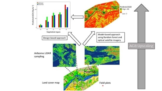
2. Material and Methods
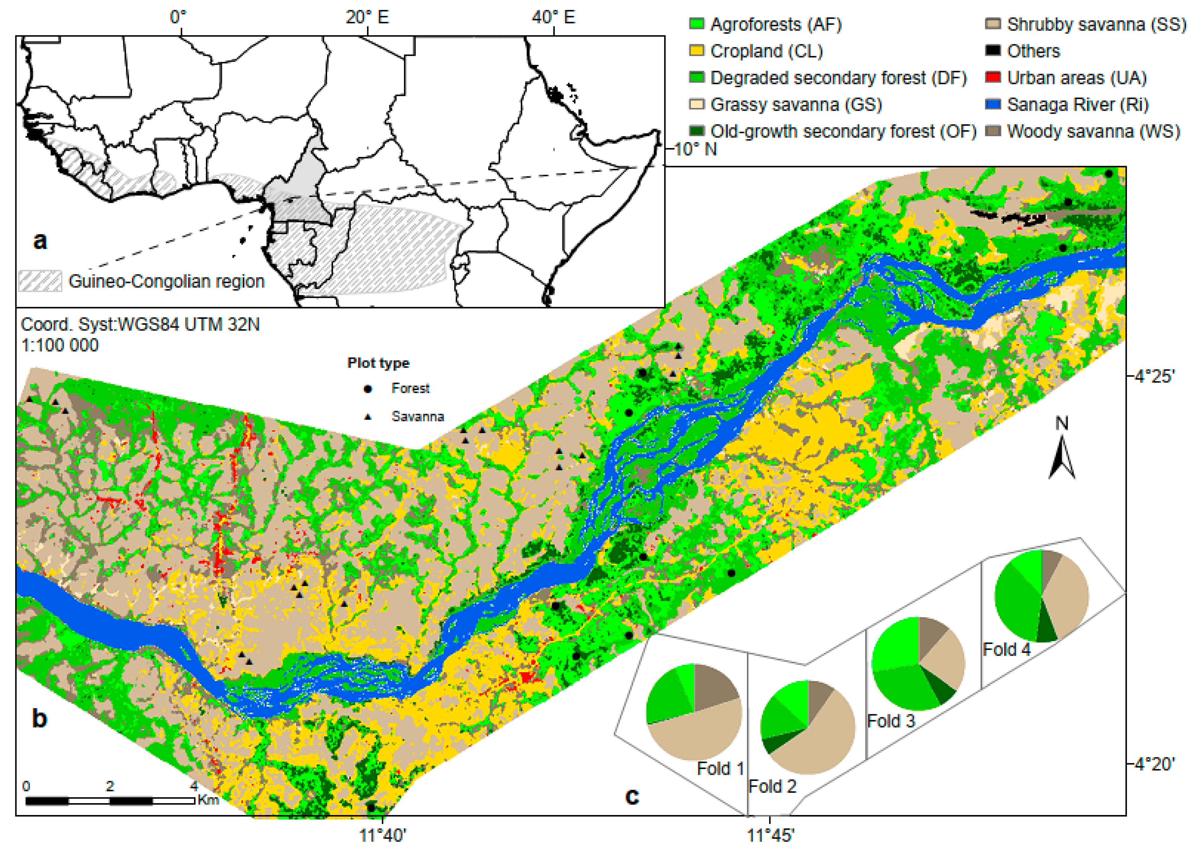
2.1. Study Site

The field site is crossed by the Sanaga river and falls within a forest-savanna mosaic of the Guineo–Congolian region with gallery forests along the river courses [27] and covers an area of 216 km2 (4° 00’–4° 30’ N and 11° 30’–12° 00’ E; Figure 1a).
The area is under the influence of an equatorial climate of Guinean type [28], which is hot and humid with an average annual temperature of 25 °C. Mean annual rainfall is 1,500 mm, with a rainfall distribution characterized by a dry season lasting over three months (December–March), during which the monthly rainfall is less than 70 mm. The average altitude is 600 m. Dominating soil types in the area are ferralitic and hydromorphic soils [29]. The area is a target for small- and large-scale agriculture (artisanal cocoa farms, palm plantations) and industrial activities (e.g. hydroelectric dam construction), leading to a strong anthropogenic pressure on, for instance, the vegetation structure [30].
The vegetation is dominated by savanna formations (dominated by pyrophylous savanna species Terminalia glaucescens Planch. ex Benth; Annona senegalensis Pers.; Bridelia ferruginea Benth.) interspersed by gallery forests or semi-deciduous forests where Triplochiton scleroxylon K. Schum. and Terminalia superba Engl. & Diels dominate. Land cover classes comprising a woody component of significant AGB are agroforests (AF), degraded secondary forests (DF), old-growth secondary forests (OF), shrubby savanna (SS), and woody savanna (WS) (Figure 1c). Their proportions vary across the study area, with a higher proportion of AF, DF, and OF in the East (folds 3 and 4) and a higher proportion of SS and WS in the Western part (folds 1 and 2; Figure 1b,c).

2.2. Data Acquisition and Processing

The general methodology used in in upscaling aboveground biomass from plot scale to satellite scale with model-based and design-based approaches is presented in Figure 2.

2.2.1. Field Inventory Data

Field data acquisition campaigns were conducted from February to December 2018. We established eighteen 0.16-ha plots in savannas and eleven 1-ha plots in forests. Field plots in savanna were set along a tree density gradient, from open grassy savanna to closed woody savanna [31] (Figure 1c). Savanna plots size (i.e., 40 × 40 m) was set so as to sample relatively homogenous vegetation structure within each plot, given the high spatial heterogeneity of the vegetation in this ecosystem. Forest plots had a standard 1-ha (100 m × 100 m) area, and were distributed among the main types of closed-canopy vegetations found in the area (see Figure 1b and Section 2.1). Plots geolocation was recorded with a Trimble Geo7X Global Navigation Satellite System (GNSS) receiver, by collecting a point every 20 m along each plot contour in order to increase geolocation accuracy [7]. In each plot, the diameter at breast height (DBH; in cm) was measured for all trees with DBH ≥ 10 cm. Trees were identified in the field by expert botanists, and herbarium specimens were collected on each species for cross-identification at the herbarium of Université Libre de Bruxelles (BRLU). In savanna plots, the height (H) of all trees with DBH ≥ 10 cm was measured using a graduated pole for short trees (H ≤ 7 m) and a laser range finder device (Trupulse 360”R) for taller trees (> 7 m). In forest plots, tree height was measured on a subsample of trees per plot (approximately 50 sampled along the DBH range) with their crown apex visible using the laser range finder device. We subsequently used the BIOMASS R package [32] to fit plot-level height-diameter allometric models via a three-parameter Weibull function and predict the height of unmeasured trees. In total, we censused 4309 trees in the forests, belonging to 150 species, and 3487 trees in the savanna from 43 species. In the following analyses, we used the savanna plot size (40 × 40 m) as our minimum mapping unit, and thus split each 1-ha forest plots in four subplots of 40 * 40 m (selecting each time the subplots located on the external edge of the 1-ha plots; Appendix A). The field dataset thus consisted in 62 field plots (18 and 44 plots in savanna and forests, respectively). Table 2 presents a summary statistics of the 62 plots data installed in forest and savanna sites.

2.2.2. Airborne LiDAR Data

Airborne LiDAR Scanning data were acquired in 2012 with a Riegl LMQ-560 sensor mounted on an airplane of type Pilatus PC6 with a flight height of 600 m above ground level and an average ground speed of 167 km.h−1. The scan angle was 60° with a band swath of 690 m and 50% of overlap among adjacent flight lines which resulted in an average point density of 8.4 points.m−2. The ALS point error was 10 cm vertically and 15 cm horizontally. We used the lidR R package (v2.0.2; [33]) to process the ALS point cloud and generated a 2-m resolution canopy height model (CHM).

2.2.3. Spaceborne Data

We considered three multispectral sensors, namely Spot 6-7, Landsat 8, and Sentinel 2. Among cloud-free images in sensors archives, we looked for dry-season images acquired: (i) at (approximately) the same date (to mitigate cross-sensor differences associated to change in land cover or vegetation phenology); and (ii) as close as possible to the ALS acquisition date. The year 2015 matched our criteria and we collected Level-1C images for Spot 6/7 (acquired on January 9th, Row/Column 4912/3514), Landsat 8 (acquired on 1 December; Path/Row 185/057) and Sentinel 2B (acquired on December 19th mosaic of T32NQK & T32NRL).
We processed spaceborne optical data using the Overland algorithms [34]. Overland is a satellite image processing chain developed by AIRBUS DS Geo which aims to produce cloud and shadow masks and perform image atmospheric corrections, especially for areas with a high degree of cloudiness like western Central Africa. It is primarily coded in the IDL language (Harris) for image processing algorithms, with a core scene model and model inversion engine that has been developed in Matlab (MatWorks) Overland uses look-up tables from LOWTRAN and performs an inversion of a coupled atmospheric scene model [35] to estimate atmospheric parameters and discard influences from sky, aerosols, and clouds on the surface reflectance. Another feature of Overland is the ability to partition the reflectance of individual pixels into respective contributions of soil, photosynthetic vegetation (green matter), and the non-photosynthetic matter (dead wood), and characterize the self-cast shadows of the rough vegetation canopies. For this, it implements a vegetation model by combining PROSPECT [36], SAIL [37], and a soil model. By inverting this vegetation model, we can notably derive the fractional cover of green vegetation (fCover), the canopy shade factor (CSF), and the leaf area index (LAI).
To predict vegetation AGB, we considered the three variables provided by Overland, as well as images spectral bands and vegetation indices from corrected images summarized in Table 3. The dataset of spaceborne optical variables thus consisted of 11 variables for Spot 6/7, 13 variables for Landsat 8 and 24 variables for Sentinel 2.

2.3. Upscaling AGB from Field to Spaceborne Measurements

2.3.1. Field-Based AGB Estimates

We used the R BIOMASS package [32], which relies on the Global Wood Density Database [38,39], to attribute to each tree a wood density (WD) value based on tree taxonomy. For trees identified at the species or genus level, the average WD of the respective taxonomic level was used. For trees identified at the family level, or unidentified trees, the plot average WD was used. We then computed tree AGB using allometric models based on DBH, H and WD. For forest trees, we used the pantropical AGB model of Chave et al. [40]. For trees from savanna plots, we used an AGB model developed for semi-arid savanna by Colgan et al. [41]. Lastly, we computed plot AGB density (AGBFIELD) as the sum of individual tree AGBs over the plot area (expressed in Mg.ha−1).

2.3.2. LiDAR-Based Reference AGB Map and Land-Cover Classification

We extracted vegetation structural metrics from the CHM (2 -m resolution) within square windows of 40 × 40 pixels so as to be an integer divisor of the size of our field plots (40 × 40 m). We computed several vegetation metrics (quantiles of pixels height distribution, canopy gap fraction, statistics of leaf area vertical distribution). These metrics allowed us to derive a simple land cover classification map (Figure 1b) via supervised classification (maximum likelihood) in Envi 5.0.
To predict vegetation AGB density from the LiDAR canopy height model, we evaluated the predictive power of a set of models using a leave-one-out cross-validation (LOO-CV) procedure. LOO-CV consists of iteratively training the model on N-1 plots (with N the total number of plots), each time withholding a different plot for testing. To account for potential autocorrelation between 0.16-ha forest subplots extracted from the same 1-ha plot (which would violate the independence hypothesis between training and test sets of the CV procedure and result in overly optimistic CV statistics), we discarded 0.16-ha forest subplots of the same 1-ha plot from the training set each time a forest subplot was tested. The vector of independent AGB predictions was then used to compute CV statistics, namely the squared correlation between AGB predictions and AGBFIELD (henceforth R2; Equation (1)) and the root mean squared prediction error (RMSPE), with:
R M S P E = i = 1 n ( y i y ^ i ) 2 n
where n is the number of plots, y i is the AGBFIELD estimate for plot i, and y ^ i is its AGB prediction.
We found that a simple linear model (Equation (2)) based on vegetation median height (MCH) yielded the best results as in [16] with an R2 of 0.81 and a RMSPE of 52.7 Mg.ha−1 (Appendix A):
A G B F I E L D = 6.27 + 8.52 × M C H  
where AGBFIELD is the plot AGB density (Mg.ha−1) derived from field data, MCH is the vegetation median height (m) over the plot on the 2 m CHM obtained in Section 2.3.2. This best LiDAR-based model was used to predict vegetation AGB over the entire study area (AGBALS map; res = 40 m) that constituted our intermediary scale for the cal/val of spaceborne-based and design-based AGB models (see next section).

2.3.3. Design-Based AGB Estimates

As a reference AGB prediction method, we followed the recommendation of the IPCC [25,49] by averaging AGB density values (either AGBALS or AGBFIELD) per (woody vegetation) land cover class. In the case of ALS, the area was fully characterized, and hence not sampled stricto sensu.

2.3.4. Model-Based AGB Estimates

Imagery products from the different satellite sensors were co-aligned to the AGBALS raster and aggregated to 40 m resolution. We used the Random Forest (RF) algorithm [50] implemented in the randomForest R package [51] to model vegetation AGB density from spaceborne optical variables. RF is a popular machine learning technique in remote sensing studies due to its ability to handle high-dimensional datasets, to account for non-linear relationships between response and predictor variables, and to its relative robustness to multicollinearity, model overparameterization, and overfitting [52]. Here, we built several RF models, considering each time a different set of spaceborne optical variables (i.e., from Spot 6/7, Landsat 8, or Sentinel 2) and using either field-based AGB estimations (strategy 1, henceforth RFFIELD) or the LiDAR-based AGBALS map (strategy 2, henceforth RFALS) for model specification and training. We then evaluated the predictive power of the RF models by comparing RF models’ predictions to independent reference AGB estimations.
Since RF have shown to overfit training data when predictors are correlated (e.g. [32,33]) or spatially auto-correlated [53], both properties being expected in our sets of optical variables, we performed a spatial forward variable selection procedure (see Appendix B). This procedure starts with no variable in the model, computes the decrease in model’s relative RMSPE (calculated by dividing the RMSPE by the mean of “observed” AGB values) that the addition of each candidate explanatory variable would lead to, and adds to the model the variable leading to the largest relative RMSPE decrease. The procedure is iterated as long as adding a supplementary variable in the model leads to relative RMSPE decrease larger than 1%. In the case of RFFIELD, the RMSPE at each iteration of the procedure was computed using a LOO-CV over the 62 AGBFIELD estimates (as in Section 2.3.2). In the case of RFALS, the number of AGBALS estimates (i.e., 117,415 pixels) makes the LOO-CV computationally prohibitive. We thus used a four-fold block CV for variable selection.

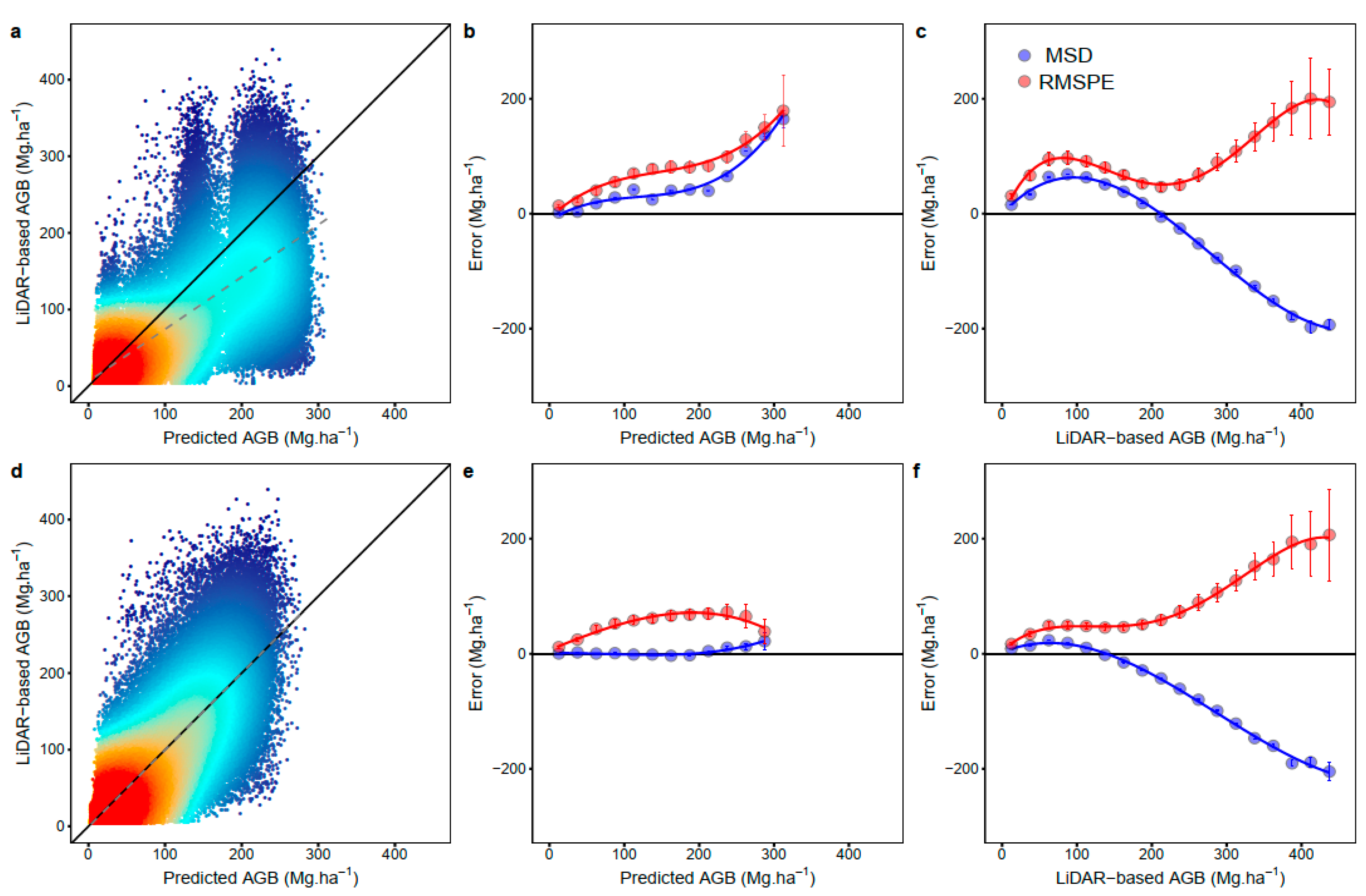
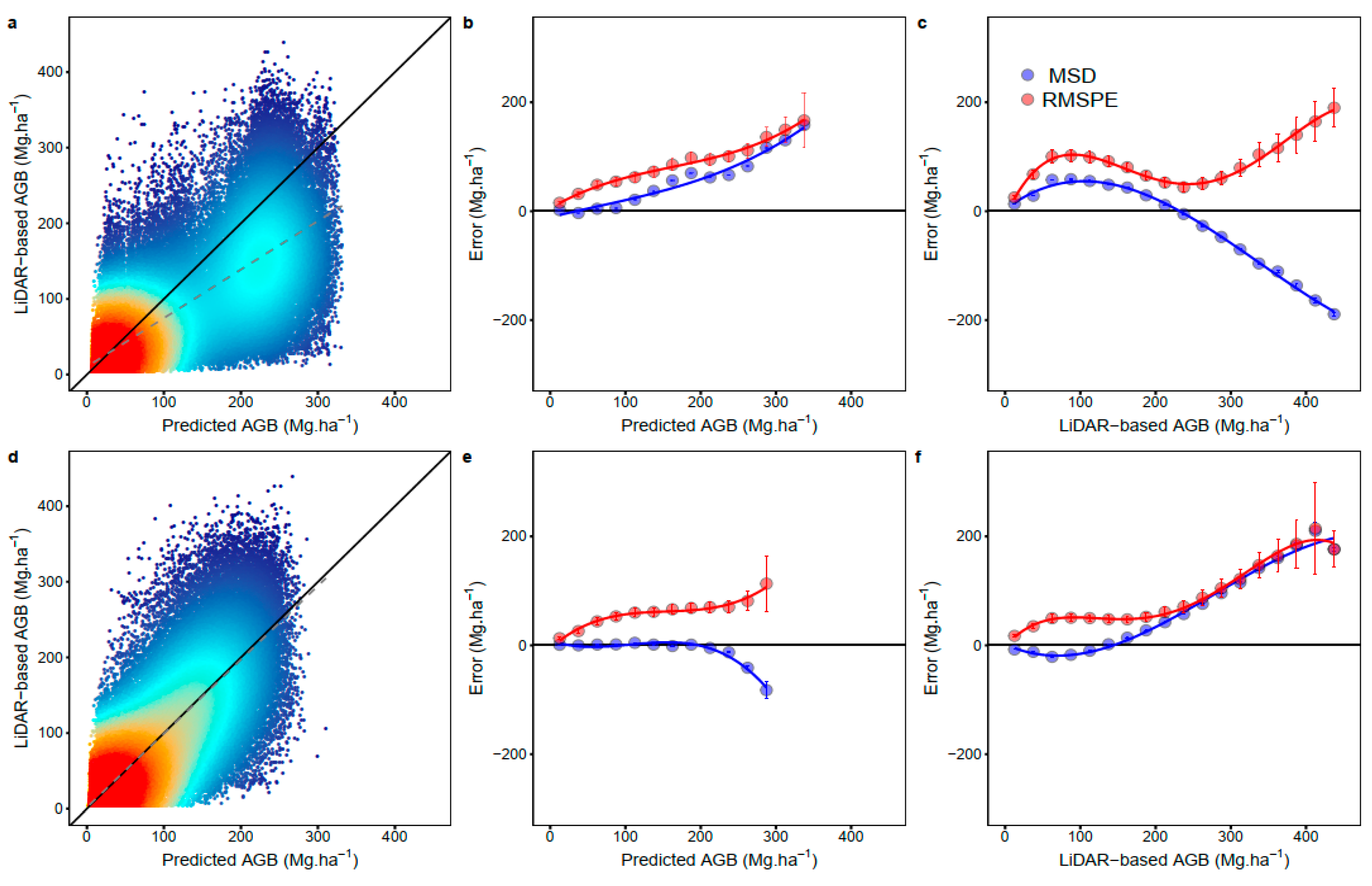
2.3.5. Four-Fold Cross-Validation

We evaluated the ability of design- and model-based approaches to predict vegetation AGB outside training areas, using the LiDAR-based AGBALS map as target AGB density values, and the four folds (blocks) defined in Figure 1c.
For design-based approaches, average AGB densities per class were assessed in the three training folds, either using ALS or field data from these folds. In the remaining fold, the mean fold AGB density was computed by multiplying the AGB density of each land cover class by its respective area, relative to the total woody vegetated area of the fold. Validation could only be performed (qualitatively) at the scale of each land cover class or the whole fold.
For model-based approaches, in the case of RFALS, we generated AGB density predictions outside training areas using the four-fold block CV. In the case of RFFIELD, to circumvent the relatively small plot number, all 62 AGBFIELD estimates were used to train the model (see LOO-CV procedure in Section 2.3.2) and generate AGB density predictions in each of the four folds. The vector of independent AGB predictions was used to compute the CV statistics as in Section 2.3.2 (i.e., R2 and RMSPE). We also computed the mean signed deviation (MSD; Equation (3)) as an indicator of model bias:
  M S D = 1 n i = 1 n ( y ^ i y i )
where n is the number of pixels, y ^ i is the AGB prediction of pixel i by RFFIELD or RFALS and y i is its AGBALS value.

3. Results

In model-based approaches, the variables selected varied depending on the training data (calibration on field AGB; RFFIELD or calibration on the intermediate AGBALS map; RFALS; see Appendix B) and satellite sensor used for model calibration. Table 4 shows the variables selected (RFFIELD & RFALS) and the model performances in cross-validation for the different models. Independently of the satellite sensor, RFFIELD models gave the poorest performances, with R2 values around 0.6, and RMSPE of up to 65 Mg.ha−1 (i.e., 90%), whereas RFALS models greatly improved the prediction accuracy (drop of ~30% in RMSPE and relative RMSPE). RFALS models based on Landsat 8 or Sentinel 2 predictors lead to a decrease of 10% both in RMSPE and relative RMSPE (R2 = 0.7; RMSPE of c. 43 Mg.ha−1 and relative RMSPE of c. 60%) compared to RFALS models based on Spot 6/7 predictors (R2 = 0.6; RMSPE = 48 Mg.ha−1 and relative RMSPE = 66.5%)
As model-based approaches provide pixelwise predictions, we can have a detailed look at the scatterplots of observed vs. predicted AGB density values in Figure 3 (for the Sentinel 2 sensor), and Appendix C & Appendix D (Spot 6-7 and Landsat 8 respectively). Concordance between predictions and observations was greatly improved, i.e., closer to the 1:1 line, for models calibrated on ALS data relative to those calibrated with field data, whereas the spaceborne sensor used seemed to make little difference. Predictions were capped around 250 Mg.ha−1 for all RFALS models. At first sight, RFFIELD models seemed capable of predictions over slightly higher AGB ranges than RFALS (point cloud extending beyond predicted AGB values > 250 Mg.ha−1 in Figure 3a), but predictions were in fact much less accurate overall and strongly biased in this upper range.
To better characterize the uncertainties of RF models estimates and possible dependence to AGB, we grouped the mean values of the RMSPE and the MSD (all in Mg.ha−1) into equally sized bins of 25 Mg.ha−1. We decomposed error and bias along the axes of both predicted and observed AGB. From a prediction perspective, RFFIELD models lead to a systematic overestimation of AGBALS (MSD > 0, hence predictions are higher than observations) across the whole predicted AGB range, with both increasing bias and error towards large AGB values (Figure 3a–c; the diagrams display model performances for Sentinel 2 predictors). This means that in any predicted AGB bin, average predictions were both largely inaccurate and imprecise when calibrating extrapolation models with field data, and all the more so at high AGB values. When binning errors along the observed AGB axis, the story was a little different, with a hinge point around 200 Mg.ha−1 below which predictions overestimated observed AGBs (MSD > 0) and above which predictions increasingly underestimated observed AGBs. RFALS models allowed a near complete bias reduction in predicted AGB values with a MSD close to zero (Figure 3d,e) along the whole range of predicted AGB values except for the highest values. In other words, despite considerable scatter, predictions were on average unbiased at the landscape level across all AGB bins up to about 200 Mg.ha−1. Along the observed AGB axis, error and bias were distributed similarly to RFFIELD, with a slightly lower hinge point.
To have a better understanding of the implication of the different AGB prediction approaches outside of training areas, we had a closer look at the distribution of predicted AGB density in the four blocks used in the 4-fold CV (Figure 4). We first investigated ALS-trained approaches. Using RFALS, (a model-based approach, based on Sentinel 2 imagery data), we could use the continuous distribution of biomass predictions. In all folds, but more markedly in the 3rd and 4th folds, the shape of the density curve diverged from the reference (ALS) curve over the higher range of AGB density values, with the expected drop around 250 Mg.ha−1. Folds 3 and 4 comprise a much higher proportion of forest vegetation than the two others (Figure 1c), which explains the difficulty of the model-based approach to faithfully reproduce de AGB density distribution. At the fold scale however (colored arrows beneath density plots), the mean predicted AGB density was close (below +/-10%) to the reference ALS value, except for the 4th fold (+13% difference). This illustrates that a well-trained statistical model, even with poor per-pixel predictive power, can provide unbiased prediction at the landscape level, at least as long as the landscape matrix is not too different from the training conditions. The design-based approach, which does not require any biomass prediction model from optical satellite predictors and ‘blindly’ applies an average LiDAR-based AGB density value to each land cover class, appeared to perform equally well, with mean AGB densities between -7.2% and +12% of the ALS reference value.
When focusing on specific land cover classes (histogram insets in Figure 4) the model-based approach, as could be expected, systematically underestimated AGB density relative to LiDAR-based estimates in the old-growth secondary forest land cover type. The expected opposite trend (overestimation) at the other end of the biomass gradient, was more subtle in low biomass vegetations such as woody savanna, with higher overestimations on the 4th fold. Design-based predictors did not present a systematic bias tendency in any vegetation type.
A similar analysis with models calibrated with AGBFIELD is presented in Appendix E. Here model-based predictions showed clearly aberrant density curves, and produced fold-level mean AGB density predictions comprised between +36.6% and +35.4% of the ALS reference. The design-based approach performed better in three folds, with meant overall AGB density below 12%, but showed a 30.9% bias in fold 3. These variations can be explained by the poor sampling rate (and design) in the training folds due to the small number of available plots, which results in some large errors in the estimation of the AGB density of some of the land cover classes (up to 100%).

4. Discussion

Transitional landscapes cover broad extents in Central Africa, and thus significantly affect the carbon budget of the continent [54]. Achieving unbiased estimation of carbon stocks and fluxes in these highly dynamic environments, characterized by mosaics of very different land uses and covers, is a critical challenge. Major climate change mitigations strategies, such as national greenhouse gas inventories (MRV-REDD+) or high carbon stock (HCS) approaches, depend on our ability to meet this challenge.
Despite known limitations, multispectral spaceborne data remain widely used for AGB extrapolations. A widely held assumption is that Airborne LiDAR scanning (ALS) data ensure better model calibration, and hence partly compensates signal limitations [14,16,18,55]. Our results indeed show that model fit and error can be drastically improved, with an R2 of 0.7 and a RMSE decrease of 30 %, when using a Random Forest model calibrated with AGBALS reference data (RFALS) instead of field plots (RFFIELD). Predictions of the latter moreover proved highly biased (inaccurate) and imprecise along the whole range of AGB densities. Looking closely at the AGB predictions of RFALS, we can however see that the signal of multispectral data, whatever the sensor, does not in fact allow accurate AGB predictions in low and high ranges of actual vegetation biomass (i.e., AGBALS). Indeed, low biomass ranges are systematically overestimated, and high biomass ranges are underestimated. This behavior has been already evidenced across the tropics [23,56] in similar studies, highlighting the fact that errors in AGB estimations when using optical signals are unfortunately still both unavoidable and crippling for large scale wall-to-wall AGB mapping [7]. It is thus important to better benchmark the values and limitations of optical signals in varying contexts through landscape-scale studies integrating highly informative ALS data. Here we showed that improved calibration of spaceborne models by ALS data did ensure unbiased estimation of AGB overall. In other words, although the signal does not allow accurate predictions of AGB in a given forest or savanna location, RFALS models still provide accurate prediction of average AGB levels across the landscape. This is only true, however, inasmuch as the balance between land cover types in the predicted landscape is comparable to that of the training area. Notably, the underestimation of total AGB will plummet with the share of land harboring high AGB forests, above the hinge point of saturation of about 225–250 Mg.ha−1. This threshold ought to be kept in mind in any further applications.
Regarding possible effects of the compromise between spatial and spectral resolution allowed by different spaceborne sensors, RFALS models based on lower spatial resolution and narrow-wavelength spaceborne images (i.e., Landsat 8 & Sentinel 2) seemed to perform slightly better than models based on higher spatial resolution broad-wavelength imagery (Spot 6/7) with a minor decrease of 10% in RMSPE. Similarly, the variability in the spectral predictors selected by our forward model selection procedure does not allow being conclusive regarding the relative interest of any given spectral index over others.
The well-accepted design-based approach, on the other end, provided a simple and accurate alternative for landscape-level AGB estimation, when trained on a dense sample of ALS data. As a single AGB value is attributed to each land cover class, this approach does not provide a detailed intra-class variation map. However, if the model-based approach does provide such a map, it is unreliable anyways, as we have shown, as long as the available predictors remain poorly correlated to AGB. It might be better not to lure the user with the pretense of a high-resolution product, when the estimates are only valid at large scale.

5. Conclusions

We showed that airborne LiDAR-based AGB data can significantly improve the calibration of prediction models from spaceborne multispectral data, with an error reduction of ~30% compared to a field-based AGB calibration. It is however crucial to acknowledge that, due to signal limitations, irrespective of the multispectral sensor and mix of spectral indices used, predictions are only unbiased at the landscape or regional level, and for land cover conditions similar to the training area. Data from upcoming new radar-based (BIOMASS, NISAR) and LiDAR-based space missions (GEDI, ICESat-2, MOLI) are expected to improve our extrapolation capacities by providing both global coverage and signals with better relationships to vegetation structure [7,57]. However, some of those valuable data will need spatial interpolation (GEDI or Ice) from optical data or will not be available for long-term monitoring. Therefore improving the use of optical data will remain an issue. Attributing average AGB density values to broad land-cover classes (referred to as design-based sampling here) will continue to remain a valid alternative to obtain regional unbiased AGB estimations.

Author Contributions

L.B.T.S., P.P. and N.B. conceived and designed the experiments. H.P. helped with image processing using the Overland processing chain. L.B.T.S. performed the experiments and analyzed the results, with the help of P.P. and N.B. L.B.T.S. wrote the first drafts of the paper and N.B., P.C., P.P., H.P. and B.S. contributed edits and advice on content. All authors have read and agreed to the published version of the manuscript.

Funding

This work is financially supported by the Nachtigal Hydropower Company (Contract n° C006C007-DES-2017) under the environmental impact study associated to the construction of a hydroelectric dam on the Sanaga River in the Central region of Cameroon. We also benefitted from the “Allocations de recherche pour une thèse au Sud (ARTS)” grant program to fund research stays in France.

Acknowledgments

We thank Moses Libalah and Eric Ngansop for botanical identification of species. We thank Bertrand Akouemo, Donatien Zebaze, Gislain Mofack, Narcisse Kamdem and Nelly Sirri for their support to field data collection. We also thank Gaëlle Viennois for image data processing in Overland software.

Conflicts of Interest

The authors declare no conflicts of interest.

Appendix A

Figure A1. (a) Illustration of data sampling within four 40 m × 40 m subplots for each 1 ha forest plots and (b) scatterplot of field-derived biomass (AGBFIELD, Mg.ha−1) vs. biomass predicted from the ALS model (AGBALS, Mg.ha−1) in the leave-one-out cross-validation. The solid black line represents the 1:1 line. AF = agroforest; DF = degraded secondary forest; OF = old-growth secondary forest; SS = shrubby savanna; WS = woody savanna plots.
Remotesensing 12 01637 g0a1

Appendix B

Figure A2. Results of the spatial forward variable selection procedure for RFFIELD model (left column) and RFALS Models (right column); (a,b) models based on Spot 6/7; (c,d) models based on Landsat 8 predictors; (e,f) models based Sentinel 2 predictors. The red dot marks the last variable leading to a decrease larger than 1% in model RMSPE.
Remotesensing 12 01637 g0a2

Appendix C

Figure A3. Performance of RF AGB prediction models (RFFIELD: top row; RFFIELD: bottom row) based on Spot 6/7 optical data. (a,d) Heat plots showing the relationships between Lidar-based AGB estimates vs. RFFIELD (panel a) and RFALS (panel d) predictions. Solid black lines represent the 1:1 line. Dashed grey lines represent the fit of simple linear models between observed and predicted AGBs (b,c,e,f). Scatterplots showing the relationships between statistics of models prediction error (namely the root mean squared prediction error, RMSPE, in red and the mean signed deviation, MSD, in blue) along the ranges of predicted AGB (panels b & e) and LiDAR-based AGB (panels c & f).
Remotesensing 12 01637 g0a3

Appendix D

Figure A4. Performance of RF AGB prediction models (RFFIELD: top row; RFFIELD: bottom row) based on Landsat 8 optical data. (a,d) Heat plots showing the relationships between Lidar-based AGB estimates vs. RFFIELD (panel a) and RFALS (panel d) predictions. Solid black lines represent the 1:1 line. Dashed grey lines represent the fit of simple linear models between observed and predicted AGBs (b,c,e,f). Scatterplots showing the relationships between statistics of model prediction error (namely the root mean squared prediction error, RMSPE, in red and the mean signed deviation, MSD, in blue) along the ranges of predicted AGB (panels b & e) and LiDAR-based AGB (panels c & f).
Remotesensing 12 01637 g0a4

Appendix E

Figure A5. Detailed analysis of model-based (Sentinel 2 sensor) and design-based AGB predictions in each fold and land-cover class, in the case of AGBFIELD trained approaches. a = Fold 1; b = Fold 2; c = Fold 3; d = Fold 4. Density curves show the distribution of LiDAR-based AGB (red) and model-based predicted AGB values (green). The arrows represent the mean AGB density values obtained by the different approaches. Inset bar plots represent mean AGB density estimates for each vegetation class. AF = agroforest; DF = degraded secondary forest; OF = old-growth secondary forest; SS = shrubby savanna; WS = woody savanna; GS = grassy savanna.
Remotesensing 12 01637 g0a5

References

  1. Ciais, P.; Bombelli, A.; Williams, M.; Piao, S.L.; Chave, J.; Ryan, C.M.; Henry, M.; Brender, P.; Valentini, R. The carbon balance of Africa: Synthesis of recent research studies. Philos. Trans. R. Soc. A Math. Phys. Eng. Sci. 2011, 369, 2038–2057. [Google Scholar] [CrossRef]
  2. Ciais, P.; Piao, S.-L.; Cadule, P.; Friedlingstein, P.; Chedin, A. Variability and recent trends in the African terrestrial carbon balance. Biogeosciences 2009, 6, 1935–1948. [Google Scholar] [CrossRef] [Green Version]
  3. Valentini, R.; Arneth, A.; Bombelli, A.; Castaldi, S.; Gatti, R.C.; Chevallier, F.; Ciais, P.; Grieco, E.; Hartmann, J.; Henry, M.; et al. A full greenhouse gases budget of Africa: Synthesis, uncertainties, and vulnerabilities. Biogeosciences 2014, 11, 381–407. [Google Scholar] [CrossRef] [Green Version]
  4. Williams, C.; Hanan, N.; Neff, J.; Scholes, R.J.; A Berry, J.; Denning, A.S.; Baker, D.F. Africa and the global carbon cycle. Carbon Balance Manag. 2007, 2, 3. [Google Scholar] [CrossRef] [PubMed] [Green Version]
  5. Richard, A.; Pekka, E.; Werner, A.; Oliver, L.; Simon, L.; Josep, G.; Robert, B.; Stephen, W.; David, A. A large and persistent carbon sink in the world’s forests. Larg. Persistent Carbon Sink World For. 2011, 333, 988–993. [Google Scholar] [CrossRef] [Green Version]
  6. Avitabile, V.; Camia, A. An assessment of forest biomass maps in Europe using harmonized national statistics and inventory plots. For. Ecol. Manag. 2018, 409, 489–498. [Google Scholar] [CrossRef] [PubMed]
  7. Réjou-Méchain, M.; Barbier, N.; Couteron, P.; Ploton, P.; Vincent, G.; Herold, M.; Mermoz, S.; Saatchi, S.; Chave, J.; De Boissieu, F.; et al. Upscaling Forest Biomass from Field to Satellite Measurements: Sources of Errors and Ways to Reduce Them. Surv. Geophys. 2019, 40, 881–911. [Google Scholar] [CrossRef]
  8. King, M.D.; Platnick, S. Spatial and Temporal Distribution of Tropospheric Clouds observed by MODIS onboard the Terra and Aqua Satellites. Four. Transform. Spectrosc. Hyperspec. Imaging Sound. Env. 2005, 51, 3826–3852. [Google Scholar] [CrossRef] [Green Version]
  9. Morton, D.C.; Nagol, J.; Carabajal, C.C.; Rosette, J.; Palace, M.; Cook, B.D.; Vermote, E.F.; Harding, D.J.; North, P. Amazon forests maintain consistent canopy structure and greenness during the dry season. Nature 2014, 506, 221–224. [Google Scholar] [CrossRef]
  10. Song, C.; Woodcock, C.E.; Seto, K.C.; Lenney, M.P.; Macomber, S.A. Classification and Change Detection Using Landsat TM Data. Remote. Sens. Environ. 2001, 75, 230–244. [Google Scholar] [CrossRef]
  11. Baccini, A.; Asner, G.P. Improving pantropical forest carbon maps with airborne LiDAR sampling. Carbon Manag. 2013, 4, 591–600. [Google Scholar] [CrossRef] [Green Version]
  12. Asner, G.P.; Mascaró, J. Mapping tropical forest carbon: Calibrating plot estimates to a simple LiDAR metric. Remote. Sens. Environ. 2014, 140, 614–624. [Google Scholar] [CrossRef]
  13. Xu, L.; Saatchi, S.S.; Shapiro, A.; Meyer, V.; Ferraz, A.; Yang, Y.; Bastin, J.-F.; Banks, N.; Boeckx, P.; Verbeeck, H.; et al. Spatial Distribution of Carbon Stored in Forests of the Democratic Republic of Congo. Sci. Rep. 2017, 7, 15030. [Google Scholar] [CrossRef] [PubMed] [Green Version]
  14. Asner, G.P. Tropical forest carbon assessment: Integrating satellite and airborne mapping approaches. Environ. Res. Lett. 2009, 4, 034009. [Google Scholar] [CrossRef]
  15. Jha, N.; Tripathi, N.K.; Chanthorn, W.; Brockelman, W.; Nathalang, A.; Pélissier, R.; Pimmasarn, S.; Ploton, P.; Sasaki, N.; Virdis, S.G.P.; et al. Forest aboveground biomass stock and resilience in a tropical landscape of Thailand. Biogeosciences 2020, 17, 121–134. [Google Scholar] [CrossRef] [Green Version]
  16. Réjou-Méchain, M.; Tymen, B.; Blanc, L.; Fauset, S.; Feldpausch, T.; Monteagudo, A.; Phillips, O.L.; Richard, H.; Chave, J. Using repeated small-footprint LiDAR acquisitions to infer spatial and temporal variations of a high-biomass Neotropical forest. Remote. Sens. Environ. 2015, 169, 93–101. [Google Scholar] [CrossRef]
  17. Adhikari, H.; Heiskanen, J.; Siljander, M.; Maeda, E.; Heikinheimo, V.; Pellikka, P.K. Determinants of Aboveground Biomass across an Afromontane Landscape Mosaic in Kenya. Remote. Sens. 2017, 9, 827. [Google Scholar] [CrossRef] [Green Version]
  18. Ordway, E.M.; Asner, G.P. Carbon declines along tropical forest edges correspond to heterogeneous effects on canopy structure and function. Proc. Natl. Acad. Sci. USA 2020, 117, 7863–7870. [Google Scholar] [CrossRef]
  19. Wang, D.; Wan, B.; Liu, J.; Su, Y.; Guo, Q.; Qiu, P.; Wu, X. Estimating aboveground biomass of the mangrove forests on northeast Hainan Island in China using an upscaling method from field plots, Uav-Lidar data and Sentinel-2 imagery. Int. J. Appl. Earth Obs. Geoinform. 2020, 85, 101986. [Google Scholar] [CrossRef]
  20. Asner, G.P.; Mascaro, J.; Anderson, C.B.; E Knapp, D.; E Martin, R.; Kennedy-Bowdoin, T.; Van Breugel, M.; Davies, S.J.; Hall, J.S.; Muller-Landau, H.C.; et al. High-fidelity national carbon mapping for resource management and REDD. Carbon Balance Manag. 2013, 8, 7. [Google Scholar] [CrossRef] [Green Version]
  21. Hirata, Y.; Furuya, N.; Saito, H.; Pak, C.; Leng, C.; Sokh, H.; Vuthy, M.; Kajisa, T.; Ota, T.; Mizoue, N. Object-Based Mapping of Aboveground Biomass in Tropical Forests Using LiDAR and Very-High-Spatial-Resolution Satellite Data. Remote. Sens. 2018, 10, 438. [Google Scholar] [CrossRef] [Green Version]
  22. Baccini, A.; Goetz, S.J.; Walker, W.S.; Laporte, N.T.; Sun, M.; Sulla-Menashe, D.; Hackler, J.; Beck, P.S.A.; Dubayah, R.; Friedl, M.A.; et al. Estimated carbon dioxide emissions from tropical deforestation improved by carbon-density maps. Nat. Clim. Chang. 2012, 2, 182–185. [Google Scholar] [CrossRef]
  23. Csillik, O.; Kumar, P.; Mascaro, J.; O’Shea, T.; Asner, G.P. Monitoring tropical forest carbon stocks and emissions using Planet satellite data. Sci. Rep. 2019, 9, 17831–17912. [Google Scholar] [CrossRef] [Green Version]
  24. Asner, G.P.; Brodrick, P.G.; Philipson, C.D.; Vaughn, N.R.; Martin, R.E.; E Knapp, D.; Heckler, J.; Evans, L.J.; Jucker, T.; Goossens, B.; et al. Mapped aboveground carbon stocks to advance forest conservation and recovery in Malaysian Borneo. Boil. Conserv. 2018, 217, 289–310. [Google Scholar] [CrossRef]
  25. Buendia, E.; Tanabe, K.; Kranjc, A.; Baasansuren, J.; Fukuda, M.; Ngarize, S.; Osako, A.; Pyrozhenko, Y.; Shermanau, P.; Federici, S. Refinement To the 2006 Ipcc Guidelines for National Greenhouse Gas Inventories; IPCC: Geneva, Switzerland, 2019. [Google Scholar]
  26. McRoberts, R.E.; Næsset, E.; Liknes, G.C.; Chen, Q.; Walters, B.; Saatchi, S.; Herold, M. Using a Finer Resolution Biomass Map to Assess the Accuracy of a Regional, Map-Based Estimate of Forest Biomass. Surv. Geophys. 2019, 40, 1001–1015. [Google Scholar] [CrossRef]
  27. Diziain, R. Word Atlas Of Agriculture; International Association of Agricultural Economists/Committee for the World Atlas of Agriculture: Novara, Italy, 1976. [Google Scholar]
  28. Djoufack, M.V.; Fonteine, B.; Tsalefac, M. Étude Multi-Echelles des Précipitations et du Couvert Végétal au Cameroun: Analyses Spatiales, Tendances Temporelles, Facteurs Climatiques et Anthropiques de Variabilité du NDVI; Université de Bourgogne et Université de Yaoundé I: Yaounde, Cameroon, 2011. [Google Scholar]
  29. Food andAgriculture Organization (FAO). Unesco Soil Map of the World 1:5 000 000; Unesco: Paris, France, 1977. [Google Scholar]
  30. Jagoret, P.; Michel-Dounias, I.; Snoeck, D.; Ngnogué, H.T.; Malézieux, E. Afforestation of savannah with cocoa agroforestry systems: A small-farmer innovation in central Cameroon. Agrofor. Syst. 2012, 86, 493–504. [Google Scholar] [CrossRef]
  31. Daget, P.; Poissonet, J. Prairies et Pâturages Méthodes d’Etude de Terrain et Interprétations; Cnrs/ Cir; Umr Selment (Systèmes d’Elevage Méditerranéens et Tropicaux): Montpellier, France, 2010; 955p. [Google Scholar]
  32. Réjou-Méchain, M.; Tanguy, A.; Piponiot, C.; Chave, J.; Hérault, B. Biomass: An package for estimating above-ground biomass and its uncertainty in tropical forests. Methods Ecol. Evol. 2017, 8, 1163–1167. [Google Scholar] [CrossRef]
  33. Jean-Romain, R.; David, A. Lidr: Airborne LiDAR Data Manipulation and Visualization for Forestry Applications. Remote Sens. 2019, 11. [Google Scholar] [CrossRef] [Green Version]
  34. Defence, A. Geoland2-BioPar Methods Compendium of MERIS FR Biophysical Products. GISci. Remote Sens. 2014, 52. [Google Scholar]
  35. Kneizys, F.X.; Shettle, E.P.; Gallery, W.O.; Chetwynd, J.H. Atmospheric Transmittance/Radiance: Computer Code Lowtran 5. Atmos. Trans. Rad. Com. Code Low. 1980. [Google Scholar]
  36. Jacquemoud, S.; Baret, F. Prpspect: A model of leaf optical properties spectra. Remote. Sens. Environ. 1990, 34, 75–91. [Google Scholar] [CrossRef]
  37. Verhoef, W. Light scattering by leaf layers with application to canopy reflectance modeling: The Sail model. Remote. Sens. Environ. 1984, 16, 125–141. [Google Scholar] [CrossRef] [Green Version]
  38. Chave, J.; Coomes, D.; Jansen, S.; Lewis, S.L.; Swenson, N.G.; Zanne, A.E. Towards a worldwide wood economics spectrum. Ecol. Lett. 2009, 12, 351–366. [Google Scholar] [CrossRef] [PubMed]
  39. Zanne, A.E.; Lopez-Gonzalez, G.; Coomes, D.A.; Ilic, J.; Jansen, S.; Lewis, S.L.; Miller, R.B.; Swenson, N.G.; Wiemann, M.C.; Chave, J.; et al. Global Wood Density Database. 2009. Available online: http://hdl.handle.net/10255/dryad.235 (accessed on 16 March 2020).
  40. Chave, J.; Réjou-Méchain, M.; Burquez, A.; Chidumayo, E.; Colgan, M.S.; Delitti, W.B.; Duque, A.; Eid, T.; Fearnside, P.M.; Goodman, R.C.; et al. Improved allometric models to estimate the aboveground biomass of tropical trees. Glob. Chang. Boil. 2014, 20, 3177–3190. [Google Scholar] [CrossRef] [PubMed]
  41. Colgan, M.S.; Asner, G.P.; Swemmer, T.; Swemmer, A. Harvesting tree biomass at the stand level to assess the accuracy of field and airborne biomass estimation in savannas. Ecol. Appl. 2013, 23, 1170–1184. [Google Scholar] [CrossRef] [PubMed]
  42. Sims, D.; Gamon, J.A. Relationships between leaf pigment content and spectral reflectance across a wide range of species, leaf structures and developmental stages. Remote. Sens. Environ. 2002, 81, 337–354. [Google Scholar] [CrossRef]
  43. Tucker, C.J. Red and photographic infrared linear combinations for monitoring vegetation. Remote Sens. Environ. 1979, 8, 127–150. [Google Scholar] [CrossRef] [Green Version]
  44. Huete, A.; Didan, K.; Miura, T.; Rodriguez, E.; Gao, X.; Ferreira, L. Overview of the radiometric and biophysical performance of the MODIS vegetation indices. Remote. Sens. Environ. 2002, 83, 195–213. [Google Scholar] [CrossRef]
  45. Jordan, C.F. Derivation of Leaf-Area Index from Quality of Light on the Forest Floor. Ecology 1969, 50, 663–666. [Google Scholar] [CrossRef]
  46. Frampton, W.J.; Dash, J.; Watmough, G.; Milton, E.J. Evaluating the capabilities of Sentinel-2 for quantitative estimation of biophysical variables in vegetation. ISPRS J. Photogramm. Remote. Sens. 2013, 82, 83–92. [Google Scholar] [CrossRef] [Green Version]
  47. Kross, A.; Seaquist, J.W.; Roulet, N.T.; Fernandes, R.; Sonnentag, O. Estimating carbon dioxide exchange rates at contrasting northern peatlands using MODIS satellite data. Remote. Sens. Environ. 2013, 137, 234–243. [Google Scholar] [CrossRef]
  48. Sharma, R.; Chakraborty, A.; Joshi, P.K. Geospatial quantification and analysis of environmental changes in urbanizing city of Kolkata. Environ. Monit. Assess. 2014, 187, 187. [Google Scholar] [CrossRef]
  49. Särndal, C.-E.; Thomsen, I.; Hoem, J.M.; Lindley, D.V.; Barndorff-Nielsen, O.; Dalenius, T. Design-Based and Model-Based Inference in Survey Sampling [with Discussion and Reply]. Scand. J. Stat. 1978, 5, 27–52. [Google Scholar]
  50. Breiman, L. Random forests. Mach. Learn. 2001, 45, 5–32. [Google Scholar] [CrossRef] [Green Version]
  51. Andy, L.; Matthew, W. Classification and Regression by randomForest. R News 2002, 2, 18–22. [Google Scholar]
  52. Mariana, B.; Lucian, D. Random forest in remote sensing: A review of applications and future directions. ISPRS J. Photogramm. Remote Sens. 2016, 114, 24–31. [Google Scholar]
  53. Meyer, H.; Reudenbach, C.; Wöllauer, S.; Nauss, T. Importance of spatial predictor variable selection in machine learning applications–Moving from data reproduction to spatial prediction. Ecol. Modell. 2019, 411. [Google Scholar] [CrossRef] [Green Version]
  54. Bouvet, A.; Mermoz, S.; Le Toan, T.; Villard, L.; Mathieu, R.; Naidoo, L.; Asner, G.P. An above-ground biomass map of African savannahs and woodlands at 25 m resolution derived from Alos Palsar. Remote. Sens. Environ. 2018, 206, 156–173. [Google Scholar] [CrossRef]
  55. Timothy, D.; Onisimo, M.; Cletah, S.; Adelabu, S.; Tsitsi, B. Remote sensing of aboveground forest biomass: A review. Trop. Ecol. 2016, 57, 125–132. [Google Scholar]
  56. Zhang, L.; Xu, M.; Qiu, S.; Li, R.; Zhao, H.; Shang, H.; Lai, C.; Zhang, W. Improving the estimate of forest biomass carbon storage by combining two forest inventory systems. Scand. J. For. Res. 2016, 32, 1–9. [Google Scholar] [CrossRef]
  57. Quegan, S.; Le Toan, T.; Chave, J.; Dall, J.; Exbrayat, J.-F.; Minh, D.H.T.; Lomas, M.; D’Alessandro, M.M.; Paillou, P.; Papathanassiou, K.; et al. The European Space Agency Biomass mission: Measuring forest above-ground biomass from space. Remote. Sens. Environ. 2019, 227, 44–60. [Google Scholar] [CrossRef] [Green Version]
Figure 1. Study site. (a) Location of the study site in the Guineo-Congolian region. (b) Supervised classification of the study area into land-use/land-cover classes (40 m resolution) and distribution of the field plots within the different vegetation types. (c) Folding of the study area in four spatial folds for cross-validation of the aboveground biomass prediction models. Proportion of the different vegetation types (with a significant woody component) located within each fold.
Remotesensing 12 01637 g001
Figure 2. General workflow of the methodology used in upscaling aboveground biomass from plot scale to satellite scale with model-based and design-based approaches.
Remotesensing 12 01637 g002
Figure 3. Performance of Random Forest (RF) AGB prediction models (RFFIELD: top row; RFALS: bottom row) based on Sentinel 2 optical data. (a,d) Heat plots showing the relationships between Lidar-based AGB estimates vs. predictions from RFFIELD (panel a) and RFALS (panel d) models. Solid black lines represent the 1:1 line. Dashed grey lines represent the fit of simple linear models between observed and predicted AGBs (b,c,e,f). Plots showing the relationships between statistics of models prediction error (namely the root mean squared prediction error (RMSPE) in red and the mean signed deviation (MSD) in blue) along the ranges of predicted AGB (panels b & e) and “observed” LiDAR-based AGB (panels c & f).
Remotesensing 12 01637 g003
Figure 4. Detailed analysis of model-based (Sentinel 2 sensor) and design-based AGB predictions in each fold and land-cover class, in ALS trained approaches. a = Fold 1; b = Fold 2; c = Fold 3; d = Fold 4. Density curves show the distribution of Lidar-based AGB (red) and model-based predicted AGB values (green). The arrows represent the mean AGB density values obtained by the different approaches. Inset bar plots represent mean AGB density estimates for each vegetation class. AF = agroforest; DF = degraded secondary forest; OF = old-growth secondary forest; SS = shrubby savanna; WS = woody savanna; GS = grassy savanna.
Remotesensing 12 01637 g004
Table 1. A selection of studies using airborne LiDAR scanning data to parameterize model-based approaches and generate wall-to-wall aboveground biomass (AGB) maps from spaceborne optical imagery. Statistics of model predictive performance (i.e., R2 and root mean square prediction error; RMSPE) are derived from a variety of model validation strategies, including: (1) withholding of a given proportion of data for model testing, with test data selected at random (strat. 1); (2) 10-fold cross validation, with random split of data into folds (strat. 2); and (3) Monte Carlo cross-validation, with random or spatial split of data into folds (strat. 3 and 4, respectively). Details of cross-validation strategies can be found in the original studies. RMSPE provided in Mg of carbon per hectare in original studies are converted to Mg of AGB per hectare with a carbon-to-AGB conversion factor of 0.5.
CountryMultispectralResolution (m)Model TypeModel ValidationR2RMSPE
(Mg.ha−1)
Ref.
Colombia & PeruMODIS500Random Foreststrat 1 (10%)0.8631.4–35.2[11]
ChinaSentinel 210Random Foreststrat 20.6250.36[19]
PanamaLandsat 5,7100Random Foreststrat 1 (30%)0.6245[20]
CambodiaQuickBird1.5Multiple regression-0.7342.8[21]
Democratic Republic of CongoLandsat 8100Maximum Entropystrat 30.7661.29[13]
strat 40.6562.16
PantropicalMODIS500Random Foreststrat 1 (10%)0.71–0.8338–50[22]
PeruPlanet Dove100Random Foreststrat 1 (20%)0.750.76[23]
Malaysian BorneoLandsat 830Deep learningstrat 20.783.2[24]
Table 2. Summary statistics of field plot data: mean (min-max).
SitesNo. Stem (ind.ha−1)Lorey’s Height (m)Basal Area (m2.ha−1)Woody Biomass (Mg.ha−1)
Forest392 (216–538)27 (24–33)28 (19–35)234 (80–422)
Savanna239 (50–550)7 (5–10)18 (12–28)21 (1–133)
Table 3. Band names and vegetation indices used to generate different aboveground biomass predictive models based on satellite data: Spot 6/7 (S. 6/7), Landsat 8 (L. 8), and Sentinel 2 (S. 2). Checked spectral bands and vegetation indices are candidate predictors retained for each model.
DesignationSpectral bandCandidate predictors
S. 6/7L. 8S. 2S. 6/7L. 8S. 2
Blue-B2B2
GreenB2B3B3xxx
RedB3B4B4xxx
Red1--B5 x
Red2--B6 x
Red3--B7 x
NIRB4B5B8xxx
Red4--B8a x
SWIR1-B6B11 xx
SWIR2-B7B12 xx
Vegetation indices
EquationsReferences
RGR(Red/Green)[42]xxx
NIRGR(NIR/Green) xxx
NDVI(NIR - Red)/(NIR + Red)[43]xxx
EVI2.5*[(NIR - Red)/(1 + NIR + 6*Red -7.5*Blue)][44]xxx
SR(NIR/RED)[45]xxx
SAVI(NIR - Red)/(NIR + Red + L)*1.5 with L = 0.5[44] x
IRECI(NIR - Red)/(Red1/Red2)[46] x
S2REP[705 + 35*(0.5*(Red3 + Red)/2) - NIR)/(Red2 - NIR)][46] x
NDVI1(NIR - Red1)/(NIR + Red1)[47] x
NDVI2(NIR - Red2)/(NIR + Red2)[47] x
NDVI3(NIR - Red3)/(NIR + Red3)[47] x
NDVI4(NIR - Red4)/(NIR + Red4)[48] x
NIR = near infra-red; Red 1, 2, 3 = red-Edge 1, 2, 3; Red 4 = NIR narrow; SWIR 1, 2 = short-wave infra-red 1, 2; RGR = red green ratio; NIRGR = near infra-red green ratio; NDVI = normalized difference vegetation index; EVI = enhanced vegetation index; SR = simple ratio; SAVI = soil-adjusted vegetation index; IRECI = inverted red-edge chlorophyll index; S2REP = Sentinel 2 red-edge position.
Table 4. Structure and performances (R2, RMSPE in Mg.ha−1 and relative RMSPE in %) of the different models selected for each spaceborne sensor. Performance metrics are based on 4-fold cross validation. Spot 6/7 (S. 6/7), Landsat 8 (L. 8), and Sentinel 2 (S. 2). CSF; canopy shade factor.
SensorRFFIELD ModelsR2RMSPERelative RMSPERFALS ModelsR2RMSPERelative RMSPE
S. 6/7Green + CSF + EVI0.586590Red + CSF + LAI0.6248.366.5
L. 8Red + SWIR 2 + SAVI0.6164.888Red + SWIR 2 + Green + fCover + EVI0.743.160
S. 2S2REP + SWIR 2 + NDVI 20.5863.285NDVI 2 + SWIR 2 + IRECI + NDVI 4 + Red + NDVI 30.742.858

