A Comparative Study of Water Indices and Image Classification Algorithms for Mapping Inland Surface Water Bodies Using Landsat Imagery


Abstract

1. Introduction
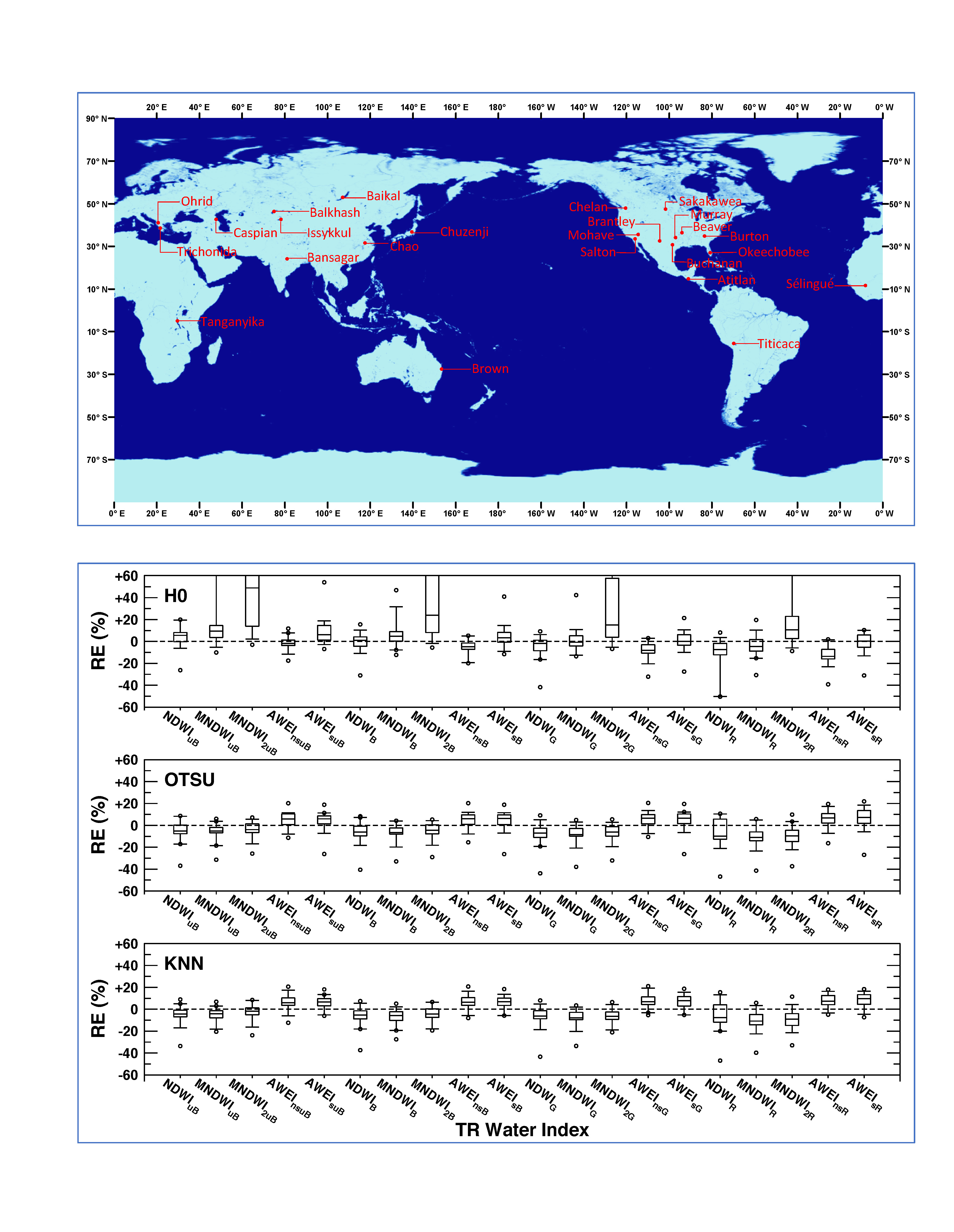
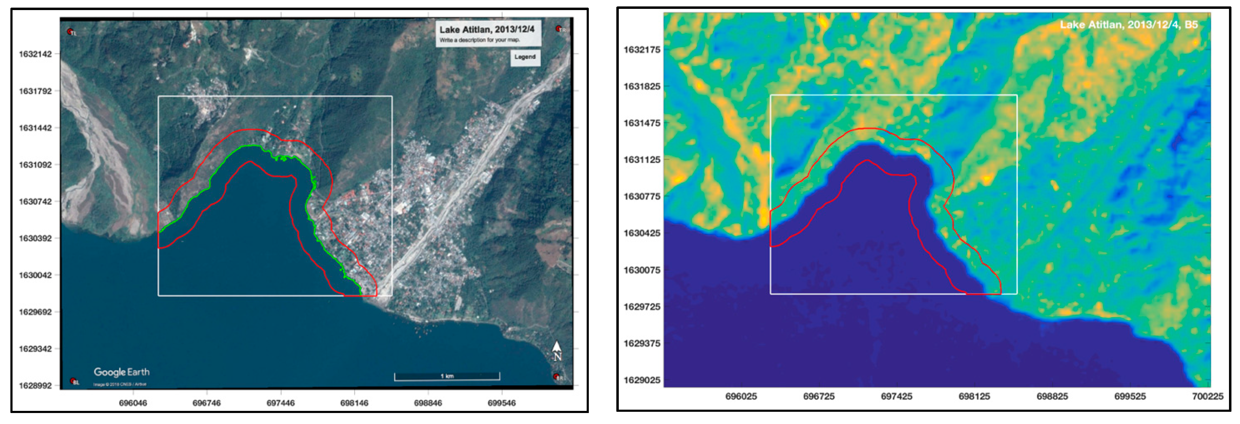
2. Study Areas and Data
3. Methods
3.1. Data Processing
3.2. Water Index
3.3. Image Classification Methods
3.3.1. Unsupervised Image Classification
3.3.2. Supervised Image Classification
3.4. Assessment of Image Classification Results
4. Results and Discussion
4.1. Impact of Different Landsat Products on Water Classification Results
4.2. Comparisons of Three Image Classification Algorithms
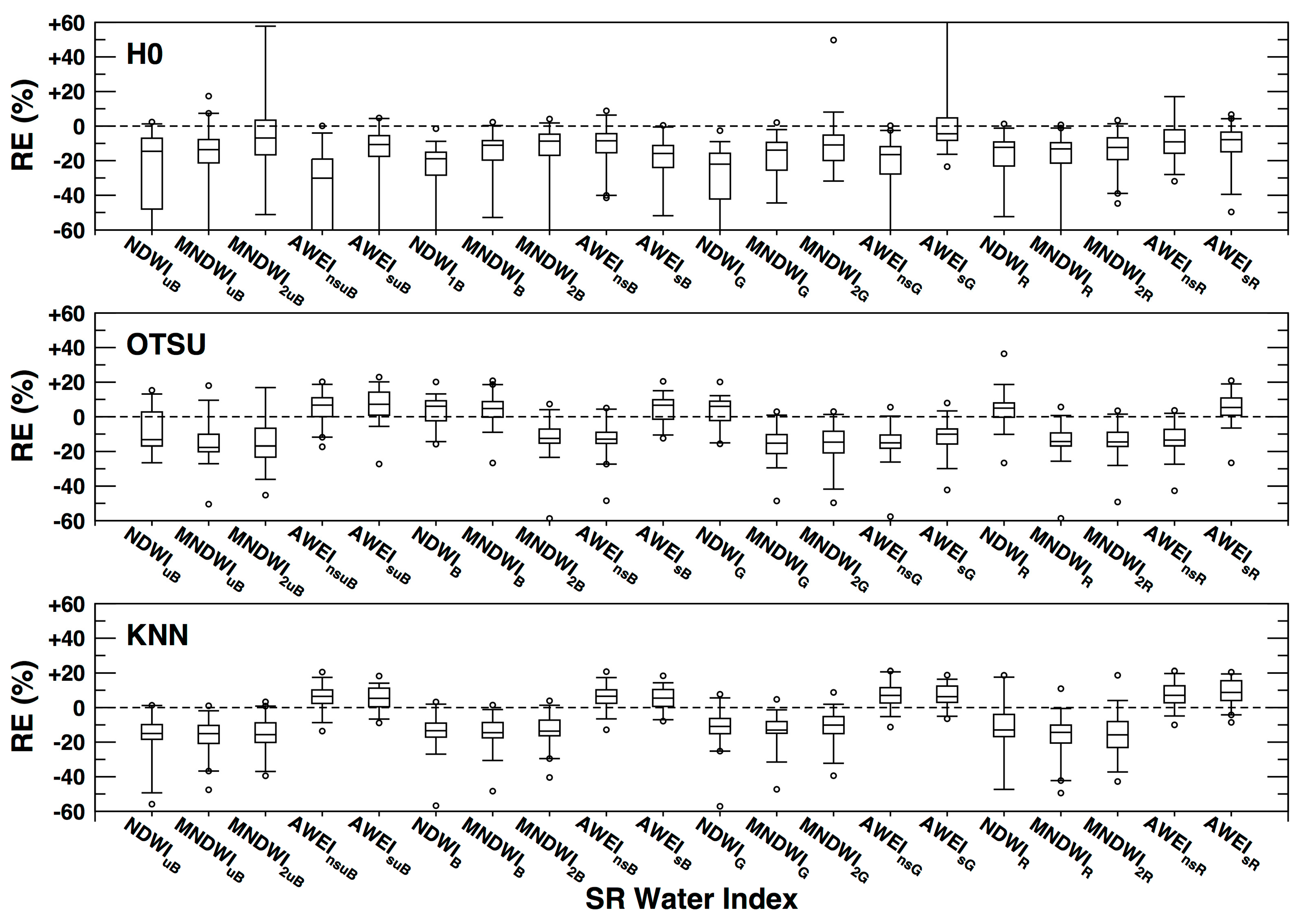
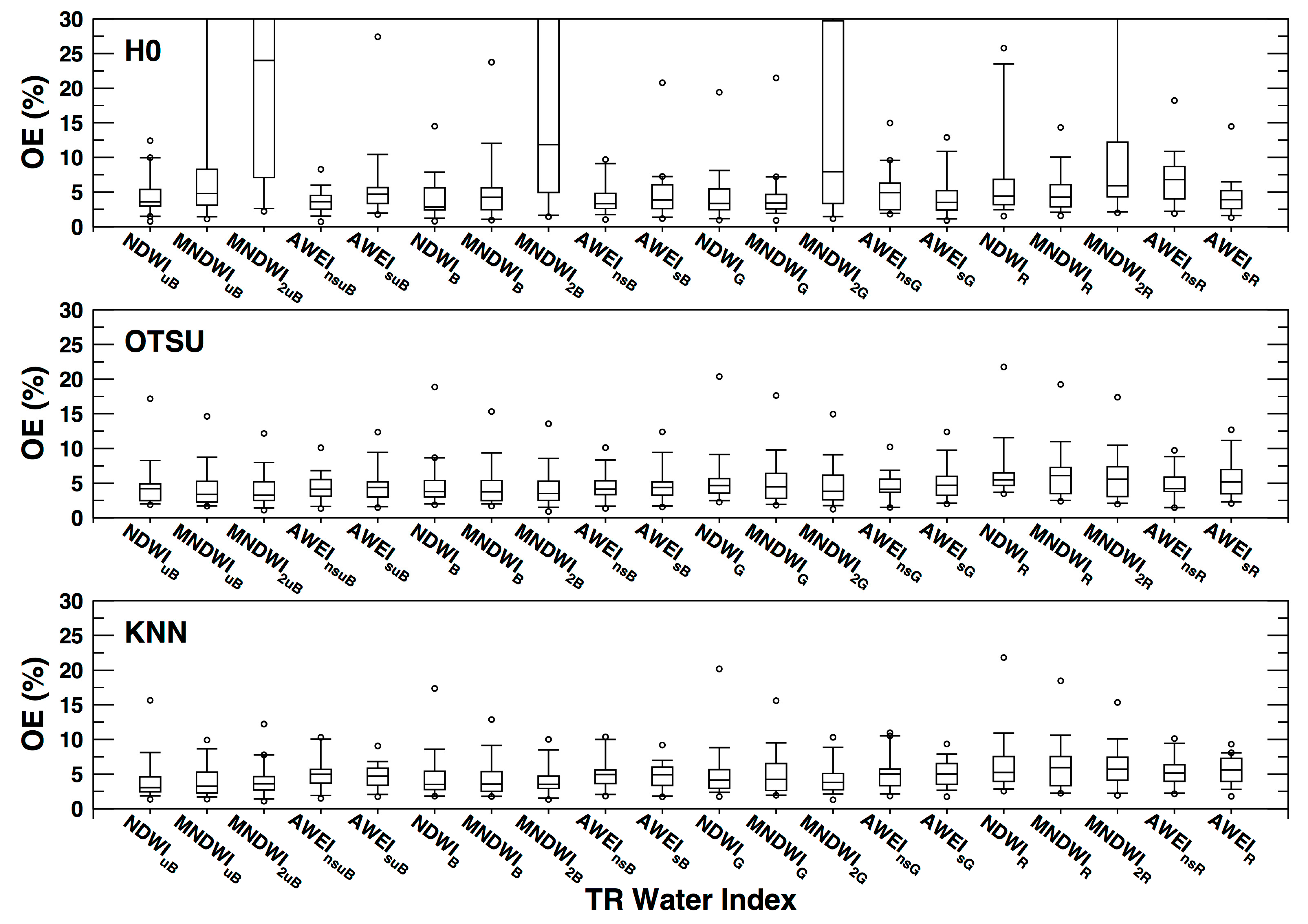
4.3. Comparisons of Twenty Water Indices
5. Conclusions
- (1)
- The top-of-atmosphere reflectance computed from the Level-1 Landsat image data are better than the current Level-2 Landsat surface reflectance products for computing water indices, because the water indices computed based on the Landsat current version Level-2 surface reflectance products might be subject to higher errors and uncertainties than the TR water indices in some regions.
- (2)
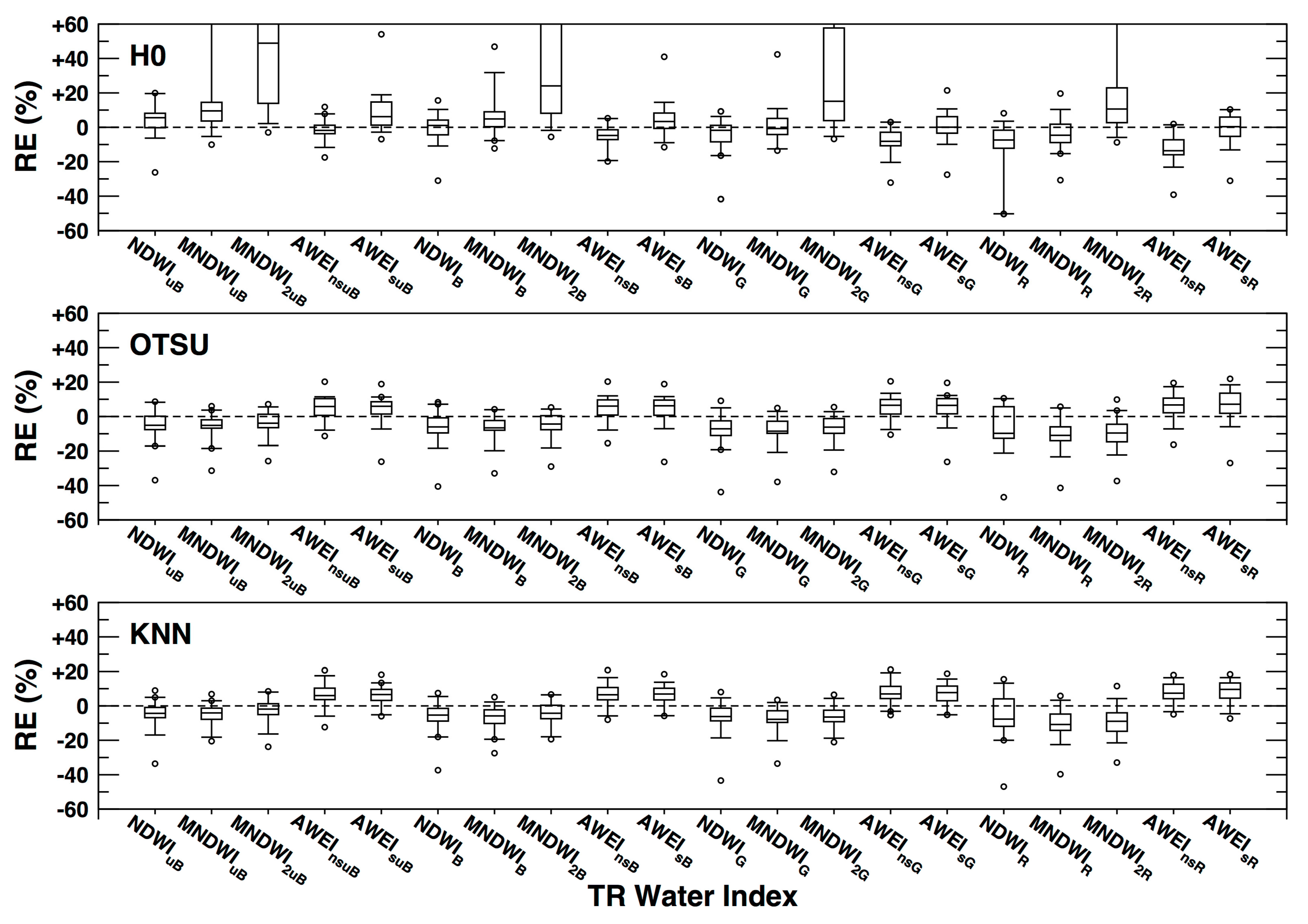
- It is not necessary to use some supervised image classification methods for identifying water bodies from Landsat imagery given the high computational cost associated with the supervised image classification methods. The unsupervised image algorithms such as the Otsu and H0 methods could yield comparable accuracy in the Landsat-extracted water body areas and image classification of water and non-water classes as the KNN method.
- (3)
- Although the zero-water index threshold (i.e., the H0 method) worked better in slightly more than 50% cases compared to the automatic threshold determined by the Otsu method, the Otsu method produced less large error outliers than the H0 method. Therefore, if there is no preference when selecting water index for classifying water and non-water classes, the Otsu method is preferable to the H0 method.
- (4)
- Among five commonly used green band-based water indices, AWEIs produced both the lowest mean absolute relative errors (MARE) in the Landsat-extracted water body areas and mean overall errors in the Landsat image classifications (MOE) for the H0 method, AWEIns produced both the lowest MARE and MOE for the Otsu method, and MNDWI2 produced both the lowest MARE and MOE for the KNN method.
- (5)
- Comparisons among twenty water indices over 24 lakes across the globe showed that the ultra-blue band-based AWEInsuB is the best water index for the H0 method, and the ultra-blue band-based MNDWI2uB is the best water index for both the Otsu and KNN methods.
Supplementary Materials
Author Contributions
Funding
Acknowledgments
Conflicts of Interest
References
- Allen, G.H.; Pavelsky, T.M. Global extent of rivers and streams. Science 2018, 361, 585–588. [Google Scholar] [CrossRef] [PubMed]
- Shiklomanov, I.A.; Sokolov, A.A. Methodological Basis of Water Balance Investigation and Computation. Available online: http://hydrologie.org/redbooks/a148/iahs_148_0077.pdf (accessed on 16 April 2020).
- Dingman, S.L. Physical Hydrology, 3rd ed.; Waveland Press, Inc.: Long Grove, IL, USA, 2015; p. 643. [Google Scholar]
- Hornberger, G.M.; Wiberg, P.L.; Raffensperger, J.P.; D’Odorico, P. Elements of Physical Hydrology, 2nd ed.; Johns Hopkins University Press: Baltimore, MD, USA, 2014; p. 378. [Google Scholar]
- Overton, I.C. Modeling floodplain inundation on a regulated river: Integrating GIS, remote sensing and hydrological models. River Res. Appl. 2005, 21, 91–101. [Google Scholar] [CrossRef]
- Matgen, P.; Schumann, G.; Henry, J.P.; Hoffmann, L.; Pfister, L. Integration of SAR derived river inundation areas, high-precision topographic data and a river flow model toward near real-time flood management. Int. J. Appl. Earth Obs. Geoinf. 2007, 9, 247–263. [Google Scholar] [CrossRef]
- Khan, S.I.; Hong, Y.; Wang, J.; Yilmaz, K.K.; Gourley, J.J.; Alder, R.F.; Brakenridge, G.R.; Policelli, F.; Habib, S.; Irwin, D. Satellite remote sensing and hydrologic modeling for flood inundation mapping in Lake Victoria Basin: Implications for hydrologic prediction in ungauged basins. IEEE Trans. Geosci. Remote Sens. 2011, 49, 85–95. [Google Scholar] [CrossRef]
- Ban, H.; Kwon, Y.; Shin, H.; Ryu, H.; Hong, S. Flood monitoring using satellite based RGB composite imagery and refractive index retrieval visible and near-infrared bands. Remote Sens. 2017, 9, 313. [Google Scholar] [CrossRef]
- Pelletier, J.D.; Mayer, L.; Pearthree, P.A.; House, P.K.; Demsey, K.A.; Klawon, J.E.; Vincnet, K.R. An integrated approach to flood hazard assessment on alluvial fans using numerical modeling, field mapping, and remote sensing. Geol. Soc. Am. Bull. 2005, 117, 1167–1180. [Google Scholar] [CrossRef]
- Sanyal, J.; Lu, X. Remote sensing and GIS-based flood vulnerability assessment of human settlements: A case study of Gangetic West Bengal, India. Hydrol. Process. 2005, 19, 3699–3716. [Google Scholar] [CrossRef]
- Sakamoto, T.; Van Nguyen, N.; Kotear, A.; Ohno, H.; Ishitsuka, N.; Yokozawa, M. Detecting temporal changes in the extent of annual flooding within the Cambodia and the Vietnamese Mekong Delta from MODIS time-series imagery. Remote Sens. Environ. 2007, 109, 295–313. [Google Scholar] [CrossRef]
- Taubenbock, H.; Wurm, M.; Netzband, M.; Zwenzner, H.; Roth, A.; Rahman, A.; Dech, S. Flood risks in urbanized areas-multi-sensoral approaches using remotely sensed data for risk assessment. Nat. Hazards Earth Syst. Sci. 2011, 11, 431–444. [Google Scholar] [CrossRef]
- Skakun, S.; Kussul, N.; Shelestov, A.; Kussui, O. Flood hazard and flood risk assessment using a time series of satellite images: A case study in Namibia. Risk Anal. 2014, 34, 1521–1537. [Google Scholar] [CrossRef]
- Rahman, M.S.; Di, L. The state of the art of spaceborne remote sensing in flood management. Nat. Hazards 2017, 85, 1223–1248. [Google Scholar] [CrossRef]
- Rosser, J.F.; Leibovici, D.G.; Jackson, M.J. Rapid flood inundation mapping using social media, remote sensing an topographic data. Nat. Hazards 2017, 87, 103–120. [Google Scholar] [CrossRef]
- Huang, X.; Wang, C.; Li, Z. Reconstructing flood inundation probability by enhancing near real-time imagery with real-time gauges and tweets. IEEE Trans. Geosci. Remote Sens. 2018, 56, 4691–4701. [Google Scholar] [CrossRef]
- Psomiadis, E.E.; Soulis, K.X.; Zoka, M.; Decas, N. Synergistic approach of remote sensing and GIS techniques for flash-flood monitoring and damage assessment in Thessaly Plain Area, Greece. Water 2019, 11, 448. [Google Scholar] [CrossRef]
- Frappart, F.; Papa, F.; Famiglietti, J.S.; Prigent, C.; Rossow, W.B.; Seyler, F. Interannual variations of river water storage from a multiple satellite approach: A case study for the Rio Negro River basin. J. Geophys. Res.-Atmos. 2008, 113, D21104. [Google Scholar] [CrossRef]
- Cai, X.; Gan, W.; Ji, W.; Zhao, Z.; Wang, X.; Chen, X. Optimizing remote sensing-based level-area modeling of large lake wetlands: Case study of Poyang Lake. IEEE J. Sel. Top. Appl. Earth Obs. Remote Sens. 2015, 8, 471–479. [Google Scholar] [CrossRef]
- Normandin, C.; Frappart, F.; Lubac, B.; Belanger, S.; Marieu, V.; Blarel, F.; Robinet, A.; Guiastrennec-Faugas, L. Quantification of surface water volume changes in the Mackenzie Delta using satellite multi-mission data. Hydrol. Earth Syst. Sci. 2018, 22, 1543–1561. [Google Scholar] [CrossRef]
- Schwerdtfeger, J.; da Silveira, S.W.; Zeilhofer, P.; Weiler, M. Coupled ground- and space- based assessment of regional inundation dynamics to asses impact of local and upstream changes on evaporation in tropical wetlands. Remote Sens. 2015, 7, 9769–9795. [Google Scholar] [CrossRef]
- Pan, F.; Nichols, J. Remote sensing of river stage using the cross sectional inundation area-river stage relationship (IARSR) constructed from digital elevation model data. Hydrol. Process. 2012, 27, 3596–3606. [Google Scholar] [CrossRef]
- Pan, F. Remote sensing of river stage and discharge. Spie Newsroom 2013. [Google Scholar] [CrossRef]
- Pan, F.; Liao, J.; Li, X.; Guo, H. Application of the inundation area-lake level rating curves constructed from the SRTM DEM to retrieving lake levels from satellite measured inundation areas. Comput. Geosci. 2013, 52, 168–176. [Google Scholar] [CrossRef]
- Pan, F.; Wang, C.; Xi, X. Constructing river stage-discharge rating curves using remotely sensed river cross-sectional inundation areas and river bathymetry. J. Hydrol. 2016, 540, 670–687. [Google Scholar] [CrossRef]
- Ridolfi, E.; Di Francesco, S.; Pandolfo, C.; Berni, N.; Biscarini, C.; Manciola, P. Coping with extreme events: Effect of different reservoir operation strategies on flood inundation maps. Water 2019, 11, 982. [Google Scholar] [CrossRef]
- Papa, F.; Prigent, C.; Durand, F.; Rossow, W.B. Wetland dynamics using a suite of satellite observations: A case study of application and evaluation for the Indian Subcontinent. Geophys. Res. Lett. 2006, 33, L08401. [Google Scholar]
- Dadson, S.J.; Ashpole, I.; Harris, P.; Davies, H.N.; Clark, D.B.; Blyth, E.; Taylor, C.M. Wetland inundation dyanmics in a model of land surface climate: Evaluation in the Niger inland delta region. J. Geophys. Res. Atmos. 2010, 115, D23114. [Google Scholar] [CrossRef]
- Prigent, C.; Papa, F.; Aires, F.; Rossow, W.B.; Matthews, E.E. Global inundation dynamics inferred from multiple satellite observations. J. Geophys. Res. Atmos. 2007, 112, D12107. [Google Scholar] [CrossRef]
- Sheffield, J.; Ferguson, C.R.; Troy, T.J.; Wood, E.F.; McCabe, M.F. Closing the terrestrial water budget from satellite remote sensing. Geophys. Res. Lett. 2009, 36, L07403. [Google Scholar] [CrossRef]
- Shi, L.; Ling, F.; Foody, G.M.; Chen, C.; Fang, S.; Li, X.; Zhang, Y.; Du, Y. Permanent disappearance and seasonal fluctuation of urban lake area in Wuhan, China monitored with long time series remotely sensed images from 1987 to 2016. Int. J. Remote Sens. 2019, 40, 8484–8505. [Google Scholar] [CrossRef]
- Li, W.; Du, Z.; Ling, F.; Zhou, D.; Wang, H.; Gui, Y.; Sun, B.; Zhang, X. A comparison of land surface water mapping using the normalized difference water index from TM, ETM+ and ALI. Remote Sens. 2013, 5, 5530–5549. [Google Scholar] [CrossRef]
- Ronki, K.; Ahmad, A.; Selamat, A.; Hazini, S. Water feature extraction and change detection using multitemporal Landsat imagery. Remote Sens. 2014, 6, 4173–4189. [Google Scholar] [CrossRef]
- Yang, Y.; Liu, Y.; Zhou, M.; Zhang, S.; Zhan, W.; Sun, C. Landsat 8 OLI image based terrestrial water extraction from heterogeneous backgrounds using a reflectance homogenization approach. Remote Sens. Environ. 2015, 171, 14–32. [Google Scholar] [CrossRef]
- Malahlela, O.E. Inland waterbody mapping: Towards improving discrimination and extraction of inland surface water features. Int. J. Remote Sens. 2016, 37, 4574–4589. [Google Scholar] [CrossRef]
- Yang, X.; Chen, L. Evaluation of automated urban surface water extraction from Sentineel-2A imagery using different water indices. J. Appl. Remote Sens. 2017, 11, 026016. [Google Scholar] [CrossRef]
- Zhou, Y.; Dong, J.; Xiao, X.; Xiao, T.; Yang, Z.; Zhao, G.; Zou, Z.; Qin, Y. Open surface water mapping algorithms A comparison of water-related spectral indices and sensors. Water 2017, 9, 256. [Google Scholar] [CrossRef]
- Ogilvie, A.; Belaud, G.; Massuel, S.; Mulligan, M.; Le Goulven, P.; Calvez, R. Surface water monitoring in small water bodies: Potential and limits of multi-sensor Landsat time series. Hydrol. Earth Syst. Sci. 2018, 22, 4349–4380. [Google Scholar] [CrossRef]
- Bangira, T.; Alfieri, S.M.; Menenti, M.; van Niekerk, A. Comparing thresholding with machine learning classifiers for mapping complex water. Remote Sens. 2019, 11, 1351. [Google Scholar] [CrossRef]
- Schwatke, C.; Scherer, D.; Dettmering, D. Automated extraction of consistent time-variable water surfaces of lakes and reservoirs based Landsat and Sentinel-2. Remote Sens. 2019, 11, 1010. [Google Scholar] [CrossRef]
- Bartolucci, L.A.; Robinson, B.F.; Silva, L.F. Field measurements of the spectral response of natural waters. Photogramm. Eng. Remote Sens. 1977, 43, 595–598. [Google Scholar]
- Meaden, G.J.; Kapetsky, J.M. Geographical Information System and Remote Sensing in Inland Fisheries and Aquaculture; FAO Fisheries Technical Paper No.318; FAO: Rome, Italy, 1991; p. 261. [Google Scholar]
- Jensen, J.R. Introductory Digital Image Processing: A Remote Sensing Perspective, 2nd ed.; Prentice-Hall: Upper Saddle River, NJ, USA, 1995. [Google Scholar]
- McFeeters, S.K. The use of the normalized difference water index (NDWI) in the delineation of open water features. Int. J. Remote Sens. 1996, 17, 1425–1432. [Google Scholar] [CrossRef]
- Xu, H. Modification of normalized difference water index (NDWI) to enhance open water features in remotely sensed imagery. Int. J. Remote Sens. 2006, 27, 3025–3033. [Google Scholar] [CrossRef]
- Feyisa, G.L.; Meilby, H.; Fensholt, R.; Proud, S.R. Automated water extraction index: A new technique for surface water mapping using Landsat imagery. Remote Sens. Environ. 2014, 140, 23–35. [Google Scholar] [CrossRef]
- Otsu, N. A threshold selection method from gray-level histograms. IEEE Trans. Syst. Mancybernetics 1979, 9, 62–69. [Google Scholar] [CrossRef]
- Richards, J.A. Remote Sensing Digital Image Analysis: An Introduction, 5th ed.; Springer: Berlin/Heidelberg, Germany, 2013; p. 494. [Google Scholar]


| Site | Google Earth | Landsat-8 OLI | ||||||
|---|---|---|---|---|---|---|---|---|
| Date | Cell | WSE * | Latitudinal Range | Longitudinal Range | Date | Path | Row | |
| Atitlan | 2013/12/04 | 3.5 m | 1558 m | 14.7274–14.7590°N | 91.1405–91.1855°W | 2013/12/04 | 20 | 50 |
| Baikal | 2013/07/22 | 4.0 m | 450 m | 53.0140–53.0593°N | 107.0193–107.1232°E | 2013/07/21 | 133 | 23 |
| Balkhash | 2014/10/10 | 4.0 m | 338 m | 46.3157–46.3551°N | 74.8289–74.9075°E | 2014/10/10 | 151 | 28 |
| Bansagar | 2014/02/20 | 3.5 m | 324 m | 24.0759–24.1072°N | 80.9680–81.0148°E | 2014/02/20 | 143 | 43 |
| Beaver | 2014/03/19 | 2.0 m | 336 m | 36.3524–36.3667°N | 93.9478–93.9707°W | 2014/03/20 | 26 | 35 |
| Brantley | 2016/03/12 | 3.0 m | 983 m | 32.5583–32.5811°N | 104.3742–104.4090°W | 2016/03/12 | 31 | 37 |
| Brown | 2016/04/19 | 2.0 m | 56 m | 27.4832–27.4978°S | 153.4223–153.4450°E | 2016/04/19 | 89 | 79 |
| Buchanan | 2014/01/13 | 4.0 m | 304 m | 30.7729–30.8028°N | 98.4219–98.4667°W | 2014/01/13 | 28 | 39 |
| Burton | 2014/10/22 | 3.0 m | 569 m | 34.8247–34.8504°N | 83.5408–83.5842°W | 2014/10/22 | 18 | 36 |
| Caspian | 2016/08/03 | 3.5 m | −29 m | 42.5993–42.6273°N | 47.7777–47.8241°E | 2016/08/03 | 168 | 30 |
| Chao | 2017/07/27 | 3.0 m | 5 m | 31.5708–31.5945°N | 117.5209–117.5598°E | 2017/07/28 | 121 | 38 |
| Chelan | 2014/07/14 | 3.0 m | 336 m | 48.0300–48.0541°N | 120.3585–120.4081°W | 2014/07/14 | 46 | 26 |
| Chuzenji | 2017/07/10 | 4.0 m | 1271 m | 36.7150–36.7544°N | 139.4568–139.5245°E | 2017/07/10 | 107 | 35 |
| Issykkul | 2013/08/31 | 4.0 m | 1603 m | 42.5661–42.6077°N | 78.1267–78.2045°E | 2013/08/31 | 148 | 30 |
| Mohave | 2015/01/13 | 3.0 m | 198 m | 35.4921–35.5166°N | 114.6591–114.6962°W | 2015/01/13 | 39 | 35 |
| Murray | 2016/01/28 | 3.0 m | 228 m | 34.0811–34.1062°N | 97.0776–97.1164°W | 2016/01/28 | 27 | 36 |
| Ohrid | 2015/07/14 | 3.0 m | 690 m | 41.0126–41.0444°N | 20.6104–20.6684°E | 2015/07/14 | 186 | 31 |
| Okeechobee | 2017/02/11 | 5.0 m | 2 m | 26.9826–27.0357°N | 80.9090–80.9756°W | 2017/02/11 | 15 | 41 |
| Sakakawea | 2016/08/01 | 3.0 m | 560 m | 47.5413–47.5680°N | 101.7566–101.8110°W | 2016/08/01 | 33 | 27 |
| Salton | 2016/10/13 | 3.5 m | −70 m | 33.4696–33.5003°N | 115.9332–115.8825°W | 2016/10/14 | 39 | 37 |
| Sélingué | 2014/01/26 | 3.0 m | 345 m | 11.5978–11.625°N | 8.1443–8.1826°W | 2014/01/27 | 199 | 52 |
| Tanganyika | 2017/06/30 | 3.0 m | 768 m | 4.8932–4.9134°S | 29.5851–29.6130°E | 2017/07/01 | 172 | 63 |
| Titicaca | 2013/08/31 | 4.0 m | 3819 m | 15.5053–15.5372°S | 69.8433–69.8889°W | 2013/09/01 | 2 | 71 |
| Trichonida | 2013/09/28 | 4.0 m | 11 m | 38.5043–38.5481°N | 21.6065–21.6836°E | 2013/09/28 | 184 | 33 |
| Error | TR WI vs. SR WI for H0 | TR WI vs. SR WI for Otsu | TR WI vs. SR WI for KNN | ||||||
|---|---|---|---|---|---|---|---|---|---|
| Better | Worse | Same | Better | Worse | Same | Better | Worse | Same | |
| RE | 353 (74%) | 127 (26%) | 0 (0%) | 375 (78%) | 104 (22%) | 1 (0%) | 360 (75%) | 115 (24%) | 5 (1%) |
| OE | 348 (73%) | 132 (27%) | 0 (0%) | 377 (78%) | 94 (20%) | 9 (2%) | 360 (75%) | 117 (24%) | 3 (1%) |
| Error | H0 vs. Otsu | H0 vs. KNN | Otsu vs. KNN | ||||||
|---|---|---|---|---|---|---|---|---|---|
| Better | Worse | Same | Better | Worse | Same | Better | Worse | Same | |
| RE | 255 | 224 | 1 | 252 | 227 | 1 | 210 | 266 | 4 |
| OE | 255 | 224 | 1 | 258 | 220 | 2 | 220 | 252 | 8 |
| Water Index | H0 | Otsu | KNN | ||||
|---|---|---|---|---|---|---|---|
| MARE (%) | MOE (%) | MARE (%) | MOE (%) | MARE (%) | MOE (%) | ||
| Ultra-blue band based | NDWIuB | 7.41 | 4.53 | 7.67 | 4.42 | 6.82 | 4.10 |
| MNDWIuB | 16.81 | 8.26 | 7.24 | 4.18 | 6.39 | 3.98 | |
| MNDWI2uB | 51.61 | 24.94 | 6.64 | 3.98 | 5.49 | 3.89 | |
| AWEInsuB | 4.86 | 3.59 | 6.80 | 4.34 | 7.65 | 4.81 | |
| AWEIsuB | 9.30 | 5.71 | 7.12 | 4.51 | 7.12 | 4.59 | |
| Blue band based | NDWIB | 5.97 | 3.89 | 8.56 | 4.76 | 7.70 | 4.44 |
| MNDWIB | 8.33 | 5.10 | 8.04 | 4.49 | 7.60 | 4.32 | |
| MNDWI2B | 42.24 | 20.40 | 7.29 | 4.19 | 6.30 | 4.05 | |
| AWEInsB | 6.35 | 3.90 | 6.99 | 4.40 | 7.54 | 4.80 | |
| AWEIsB | 7.40 | 4.64 | 7.27 | 4.60 | 7.22 | 4.65 | |
| Green band based | NDWIG | 7.18 | 4.36 | 9.83 | 5.27 | 9.13 | 4.98 |
| MNDWIG | 6.90 | 4.37 | 9.65 | 5.12 | 8.98 | 4.86 | |
| MNDWI2G | 34.25 | 16.67 | 8.53 | 4.66 | 7.56 | 4.33 | |
| AWEInsG | 9.09 | 4.92 | 7.21 | 4.49 | 7.79 | 4.93 | |
| AWEIsG | 6.41 | 4.09 | 7.97 | 4.93 | 7.92 | 4.99 | |
| Red band based | NDWIR | 12.02 | 6.42 | 12.01 | 6.57 | 11.01 | 6.27 |
| MNDWIR | 8.63 | 4.89 | 12.30 | 6.30 | 11.79 | 6.08 | |
| MNDWI2R | 23.73 | 12.20 | 11.46 | 5.96 | 10.92 | 5.75 | |
| AWEInsR | 13.27 | 6.77 | 7.78 | 4.79 | 8.18 | 5.13 | |
| AWEIsR | 6.99 | 4.25 | 9.41 | 5.65 | 8.95 | 5.49 | |
© 2020 by the authors. Licensee MDPI, Basel, Switzerland. This article is an open access article distributed under the terms and conditions of the Creative Commons Attribution (CC BY) license (http://creativecommons.org/licenses/by/4.0/).
Share and Cite
Pan, F.; Xi, X.; Wang, C. A Comparative Study of Water Indices and Image Classification Algorithms for Mapping Inland Surface Water Bodies Using Landsat Imagery. Remote Sens. 2020, 12, 1611. https://doi.org/10.3390/rs12101611
Pan F, Xi X, Wang C. A Comparative Study of Water Indices and Image Classification Algorithms for Mapping Inland Surface Water Bodies Using Landsat Imagery. Remote Sensing. 2020; 12(10):1611. https://doi.org/10.3390/rs12101611
Chicago/Turabian StylePan, Feifei, Xiaohuan Xi, and Cheng Wang. 2020. "A Comparative Study of Water Indices and Image Classification Algorithms for Mapping Inland Surface Water Bodies Using Landsat Imagery" Remote Sensing 12, no. 10: 1611. https://doi.org/10.3390/rs12101611
APA StylePan, F., Xi, X., & Wang, C. (2020). A Comparative Study of Water Indices and Image Classification Algorithms for Mapping Inland Surface Water Bodies Using Landsat Imagery. Remote Sensing, 12(10), 1611. https://doi.org/10.3390/rs12101611