Article

Water Quality Properties Derived from VIIRS Measurements in the Great Lakes

1
National Oceanic and Atmospheric Administration, National Environmental Satellite, Data, and Information Service, Center for Satellite Applications and Research, E/RA3, 5830 University Research Court, College Park, MD 20740, USA
2
Cooperative Insititute for Research in the Atmosphere at Colorado State University, Fort Collins, CO 80523, USA
*
Author to whom correspondence should be addressed.
Remote Sens. 2020, 12(10), 1605; https://doi.org/10.3390/rs12101605
Submission received: 16 April 2020 / Revised: 11 May 2020 / Accepted: 15 May 2020 / Published: 18 May 2020
(This article belongs to the Section Ocean Remote Sensing)

Abstract

:
Refined empirical algorithms for chlorophyll-a (Chl-a) concentration, using the maximum ratio of normalized water-leaving radiance nLw(λ) at the blue and green bands, and Secchi depth (SD) from nLw(λ) at 551 nm, nLw(551), are proposed for the Visible Infrared Imaging Radiometer Suite (VIIRS) onboard the Suomi National Polar-orbiting Partnership (SNPP) satellite in the Great Lakes. We demonstrated that water quality properties and phytoplankton production can be successfully monitored and assessed using the new regional Chl-a and SD algorithms, with reasonably accurate estimates of Chl-a and SD from the VIIRS-SNPP ocean color data in the Great Lakes. VIIRS-derived Chl-a and SD products using the proposed algorithms provide the temporal and spatial variabilities in the Great Lakes. Overall, Chl-a concentrations are generally low in lakes Michigan and Huron, while Chl-a data are highest in Lake Erie. The seasonal pattern shows that overall low Chl-a concentrations appear in winter and high values in June to September in the lakes. The distribution of SD in the Great Lakes is spatially and temporally different from that of Chl-a. The SD data are generally lower in summer and higher in winter in most of the Great Lakes. However, the highest SD in Lake Erie appears in summer, and lower values in winter. Significantly high values in Chl-a, and lower values in SD, in the nearshore regions, such as Thunder Bay, Saginaw Bay, and Whitefish Bay, can be related to the very shallow bathymetry and freshwater inputs from the land. The time series of VIIRS-derived Chl-a and SD data provide strong interannual variability in most of the Great Lakes.

1. Introduction

There are increasing interests in satellite algorithms to estimate water quality and biogeochemical parameters in the Great Lakes [1,2,3,4,5,6,7,8,9] for satellite ocean color sensors, e.g., the Coastal Zone Color Scanner (CZCS) [10,11], the Sea-viewing Wide Field-of-view Sensor (SeaWiFS) [12], the Moderate Resolution Imaging Spectroradiometer (MODIS) [13] on the Terra and Aqua satellites, and the Visible Infrared Imaging Radiometer Suite (VIIRS) [14] on the Suomi National Polar-orbiting Partnership (SNPP) and National Oceanic and Atmospheric Administration (NOAA)-20. Ocean color satellite observations provide important contributions in monitoring and investigating optical, biological, biogeochemical and water quality properties in global inland freshwater systems.
The ocean chlorophyll-type (OCx) approach, using the maximum band ratio (MBR) of the normalized water-leaving radiance spectra nLw(λ) (or the remote sensing reflectance spectra Rrs(λ)) from the satellite ocean color sensor at blue to green wavelengths, is generally used to derive chlorophyll-a (Chl-a) data in the global ocean waters, as the standard in NASA retrieval algorithms [15] (e.g., OC2 and OC4 for SeaWiFS, OC3M for MODIS, and OC3V for VIIRS). However, several studies have reported that the standard OCx algorithms have apparent uncertainties in Chl-a concentrations in the Great Lakes [4,6,16,17,18]. These studies also proposed several regional Chl-a algorithms for the Great Lakes, but most of these Chl-a algorithms are for the individual lakes. Lesht et al. [4] have developed tuned OCx-based Chl-a algorithms for the entire Great Lakes, using the SeaWiFS and MODIS ocean color data with in-situ Chl-a measurements, and shown improved results. Water quality properties have also been investigated using satellite-derived Secchi depth (SD) data in the Great Lakes [2,19]. In fact, Binding et al. [2] developed an empirical SD algorithm for the entire Great Lakes for the various satellite ocean color sensors (e.g., CZCS, SeaWiFS, and MODIS-Aqua). However, Chl-a and SD algorithms were generated specifically for CZCS, SeaWiFS, and/or MODIS-Aqua ocean color data in the Great Lakes. Although satellite ocean color sensors measure nLw(λ) spectra [or Rrs(λ) spectra] at similar wavelengths, there are considerable differences in the satellite measurements, which can cause differences in water quality and biological/biogeochemical products derived from different satellite ocean color sensors, particularly due to sensor spectral response function differences [20]. Therefore, it is desirable to improve the retrieval algorithms of biological and biogeochemical properties for other and future satellite ocean color sensors.
In this study, VIIRS-SNPP-derived nLw(λ) spectra over the Great Lakes are first evaluated and validated using the in-situ optical measurements, showing excellent comparisons between satellite-derived and in-situ-measured nLw(λ) spectra data. Second, regional Chl-a and SD algorithms for the VIIRS-SNPP ocean color data in the entire Great Lakes are developed, using in-situ Chl-a and SD data and the VIIRS-SNPP-derived ocean color products. Third, the proposed empirical Chl-a and SD algorithms are implemented to VIIRS-SNPP data from 2012 to 2019 for Chl-a and SD product data. Finally, the synoptic maps and time series of the VIIRS-SNPP-derived Chl-a and SD data are generated to investigate temporal and spatial distributions of Chl-a and SD in the Great Lakes.

2. Data and Methods

2.1. In-Situ Measurements

In-situ Chl-a and SD data, which are periodically measured in spring (April or May) and summer (August or September) by the U.S. Environmental Protection Agency (EPA) in the Great Lakes, were obtained from the Great Lake Environmental Database System (GLENDA). Specifically, in-situ Chl-a and SD data, in the periods of 2012–2015 and 2012–2018, were used to develop regional Chl-a and SD algorithms for VIIRS-SNPP ocean color applications in the Great Lakes, as well as to evaluate VIIRS-SNPP-derived Chl-a and SD products (Figure 1). Figure 1 shows locations of in-situ Chl-a (noted as “EPA Chl-a”) and SD (noted as “EPA Secchi”) over the Great Lakes.
In addition, in-situ radiometric data, including nLw(λ) (or Rrs(λ)) spectra at various VIIRS spectral bands obtained from the SeaWiFS Bio-optical Archive and Storage System (SeaBASS) database from the NASA Ocean Biology Processing Group [21], were also used to evaluate VIIRS-SNPP-derived ocean color products in the Great Lakes (Figure 1). Locations of the in-situ nLw(λ) data in SeaBASS over the Great Lakes are also shown in Figure 1, noted as “SeaBASS nLw”.

2.2. Satellite Ocean Color Data

Ocean color Environmental Data Records (EDR or Level-2 data) of VIIRS-SNPP [22] are processed using the Multi-Sensor Level-1 to Level-2 (MSL12) ocean color data processing system, with the near-infrared (NIR) and the shortwave infrared (SWIR) combined (NIR–SWIR) atmospheric correction algorithm [23,24,25,26,27,28,29]. It should be noted that VIIRS-SNPP-derived ocean color products have been well studied, evaluated, and validated for the global ocean waters, showing generally high quality ocean color product data [30,31,32,33]. The VIIRS-SNPP ocean color Level-2 data from 2012 to 2019 in the Great Lakes were used to develop the regional water quality algorithms using the in-situ measurements and VIIRS-derived water quality products. The ice masking algorithm for the Great Lakes [34] was applied to VIIRS Level-2 data, to identify ice-contaminated pixels during the winter season, and the mapped VIIRS ocean color data were generated with a Mercator projection at 1 × 1 km spatial resolution. Four Level-2 data flags, i.e., high sun glint [32,35], high sensor-zenith and solar-zenith angles [32], and straylight/cloud shadowing [36], were applied to VIIRS Level-2 data. Next, pixels (after removing the four flagged data) were extracted from the VIIRS Level-2 data around the location of in-situ measurements (a box with 5 × 5 pixels) and used for the matchup analysis. Detailed information for the satellite-in-situ data matchup procedure can be found in Wang et al. [29]. It is particularly noted that, in order to keep a good data quality of VIIRS-SNPP-derived water property data over the Great Lakes, the four flags must be applied to mask out questionable satellite retrievals [32]. This is in addition to other data masking, e.g., land and cloud masking [37].

2.3. Comparison of VIIRS-SNPP and In-Situ nLw(λ) Measurements

In order to evaluate the performance of VIIRS-derived ocean color products in the Great Lakes, in-situ radiometric measurements from the NASA SeaBASS were used. A total of 73 in-situ radiometric measurements were available for lakes Michigan and Erie in summer months (July or August) during the VIIRS-SNPP periods. Most of the in-situ radiometric data were acquired in the western area of Lake Erie during cyanobacteria bloom events [38]. Since bio-optical properties of the cyanobacteria bloom waters have significant surface radiance contributions at the NIR wavelengths, and cause some considerable uncertainties in the VIIRS-derived nLw(λ) products due to the failure of atmospheric correction, we used only the in-situ measurements in non-cyanobacteria bloom waters in the comparison of VIIRS-derived nLw(λ) spectra. After applying the flags on the VIIRS Level-2 data and performing the matchup procedure described in Section 2.2, VIIRS-derived nLw(λ) spectra are compared with the in-situ nLw(λ), at six points for the VIIRS visible bands at 410, 443, 486, 551, 638, and 671 nm, and at four points for the NIR bands at 745 and 862 nm, within ±5 h time difference. Figure 2 provides example spectra of in-situ nLw(λ) measurements with the VIIRS-derived nLw(λ) data at four non-cyanobacteria bloom stations. VIIRS-derived nLw(λ) data are well matched with the in-situ nLw(λ) data. Matchup results between the VIIRS-derived nLw(λ) and the SeaBASS in-situ nLw(λ) data, at the eight VIIRS bands (410, 443, 486, 551, 638, 671, 745, and 862 nm), are shown in Figure 3a. In addition, ratios of VIIRS-derived nLw(λ) at the wavelengths of 443, 486, 638, and 671 nm to nLw(551), which are usually inputs to retrieve water biological and biogeochemical products, are compared with those from the SeaBASS nLw(λ) data (Figure 3b). The VIIRS-derived nLw(λ) data correspond reasonably well to the in-situ-measured nLw(λ), with an overall mean ratio of 1.051. Radiance ratios in nLw(λ) of nLw(443) to nLw(551), nLw(486) to nLw(551), nLw(638) to nLw(551), and nLw(671) to nLw(551) from VIIRS retrievals are also well correlated with those from the SeaBASS measurements (ratios are 1.003, 1.162, 1.005, and 1.049, respectively).

2.4. Chl-a Algorithm for the VIIRS-SNPP in the Great Lakes

Because there are no in-situ radiometric measurements corresponding to the in-situ Chl-a data in the Great Lakes, we compare the GLENDA in-situ Chl-a measurements to the VIIRS-derived radiometric data, using the NIR–SWIR atmospheric correction algorithm in MSL12 [25,26,27]. Since there is usually significant uncertainty in bio-optical properties of coastal waters, caused by high amounts of suspended sediments, particularly in the western waters of Lake Erie during the spring season, in-situ Chl-a data, measured in shallow depth (< 10 m) and in the month of April, were excluded. Specifically, valid VIIRS-derived nLw(λ) spectra, corresponding to the in-situ Chl-a data within ±5 h time difference in the period of 2012 to 2015, are available for 93 data points. The empirical maximum band ratio approach [15] has been applied to the Great Lakes. Blue (443 or 486 nm) to green (551 nm) band nLw(λ) ratio values, from VIIRS-derived nLw(λ) spectra, are compared with in-situ Chl-a measurements. As expected, VIIRS-derived nLw(λ) ratio data have a strong relationship with the in-situ Chl-a data, with high correlation (r2 = 0.915). In fact, the fourth polynomial regression fit between the in-situ Chl-a and VIIRS-derived Rrs(λ) ratios can be expressed as
C h l - a = 10 ( a 0 + a 1   X + a 2   X 2 + a 3   X 3 + a 4   X 4 )
with
X = l o g [ M a x ( R r s ( 443 ) ,   R r s ( 486 ) ) R r s ( 551 ) ] ,
and coefficients a0, a1, a2, a3, and a4 of 0.3297, −2.6465, 1.9988, 0.5708, and −3.3033, respectively, which were derived from the best fit of the fourth polynomial regression.
VIIRS-derived Chl-a data, using the new regional Chl-a algorithm (Equation (1)) are compared with the in-situ Chl-a data for verification and evaluation. The matchup comparison results show that VIIRS-derived Chl-a data are in good agreement with the in-situ Chl-a data (Figure 4a). The mean and median ratios of the VIIRS-derived to the in-situ Chl-a data in the Great Lakes are 1.110 and 1.012, respectively. In addition, Figure 4b provides histograms of the VIIRS-derived and the in-situ Chl-a data, showing the two datasets have almost the same histogram distributions, although some differences do exist. For example, there is a small peak in Chl-a between ~2 and 3 mg/m3 from the in-situ Chl-a data, while there is no such peak in the VIIRS-derived Chl-a data (Figure 4b). It should be noted that daily VIIRS-derived Chl-a data from only May and August in 2012–2018 were used to derive the VIIRS histogram, because most of the in-situ Chl-a data were measured in the months of May and August. Total numbers of the VIIRS-derived and the in-situ-measured water Chl-a data that are used for the histograms are about 2.80 × 10⁷ and 666, respectively. Overall, the results show that the distribution of the VIIRS-derived Chl-a is well matched with that of the in-situ measurements. Indeed, as shown in the histogram results, Chl-a peaks, in both VIIRS-derived and in-situ data, are located around 0.5 mg/m3 (Figure 4b). Thus, VIIRS-derived Chl-a data, with the proposed regional Chl-a algorithm, are appropriate to the Great Lakes.

2.5. SD Algorithm for VIIRS-SNPP in the Great Lakes

Several studies have reported that SD has a strong correlation with nLw(λ) at the green band [2,39,40]. Similar to the situation with Chl-a data, we do not have the in-situ nLw(λ) data corresponding to in-situ SD data in the Great Lakes. Thus, VIIRS-derived nLw(551) data are compared with the in-situ SD data in the Great Lakes, for development of a regional SD algorithm. VIIRS-derived nLw(551) data are matched with the in-situ SD measurements from 2012 to 2017 at 147 data points. Figure 5a provides results of the matchup comparison of the VIIRS-derived nLw(551) with the in-situ SD data. The comparison results in Figure 5a show that VIIRS-derived nLw(551) are well correlated to the in-situ SD data in the Great Lakes (r2 = 0.875). Therefore, a new regional SD algorithm for the Great Lakes can be expressed as
S D = 10 ( b 0 + b 1   X + b 2   X 2 + b 3   X 3 )
where X = log[nLw(551)], and fitting coefficients of b0, b1, b2, and b3 are 0.8694, −0.9099, −0.7645, and −0.6390, respectively, which were derived from the best fit to Equation (3) using the in-situ-measured SD and the corresponding VIIRS-SNPP-derived nLw(551) data.
Figure 5b provides comparison results, of VIIRS-derived SD data using Equation (3) with those from the in-situ measurements for the Great Lakes, showing consistent SD data derived from the VIIRS-SNPP and the in-situ measurements. Indeed, the mean and median ratios of the VIIRS-SNPP-derived to the in-situ-measured SD data in the Great Lakes are 1.016 and 0.952, respectively. The histogram results of the VIIRS-derived and the in-situ SD data are also shown in Figure 5c. The distribution of the VIIRS-derived SD corresponds reasonably well to that of the in-situ SD data, even though the number of in-situ sample data may not be large enough for a solid statistical analysis.

3. Results

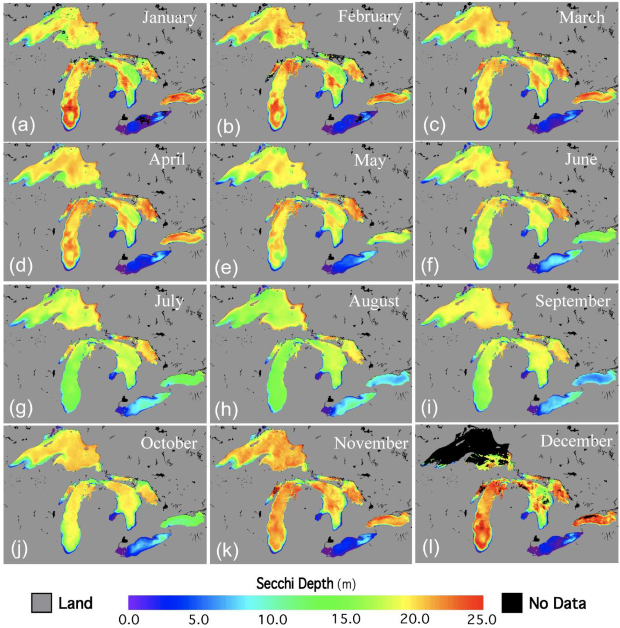
3.1. VIIRS-SNPP-Derived Monthly Climatology Chl-a and SD Images

VIIRS-derived climatology (2012–2019) monthly Chl-a images are generated using the proposed regional Chl-a algorithm (Equation (1)) in the Great Lakes (Figure 6). The images show that the highest Chl-a concentrations appear in Lake Erie in all months, unlike the other lakes.
Chl-a data in lakes Michigan and Huron are generally low, while Chl-a concentrations are relatively high in lakes Superior and Ontario. In most areas of lakes Superior, Michigan, Huron, and Ontario, Chl-a concentrations are the lowest in winter (December to February) and increase in spring. A slightly decreased Chl-a concentration appears in summer, and then Chl-a values increase in autumn. The highest Chl-a generally appears in June and September for most of the lakes. However, Chl-a patterns vary seasonally and spatially, with lakes and locations. Particularly, the seasonal distribution of Chl-a in the nearshore waters (e.g., Green Bay, Saginaw Bay, and Thunder Bay) are different from those in offshore waters of the lakes. Significantly high Chl-a concentrations in the nearshore waters are seen in spring to fall months. Seasonal distribution of Chl-a in Lake Erie is evidently different from the other lakes, showing that relatively lower Chl-a appear in June and December, and significantly high Chl-a appears in August and September. In particular, higher Chl-a in the western area of Lake Erie is apparently contrary to lower Chl-a in the eastern area.
VIIRS-derived climatology (2012–2019) monthly SD images, using the new regional SD algorithm (Equation (3)) in the Great Lakes, were also generated (Figure 7). The general spatial distribution of SD is somewhat different from that of Chl-a in most of the lakes. Specifically, SD is the highest in November and December for most areas of lakes Superior, Michigan, Huron, and Ontario, while the lowest SD values appear in the summer months (July and August), depending on the lake. In Lake Superior, SD data are apparently lower in the southwestern area, the northern area (Thunder Bay), the mid-southern area (Keweenaw Bay), and the eastern area (Whitefish Bay) during most months, compared to the main body of Lake Superior. Clearly, high SD values appear in the southern and northern areas of Lake Michigan in December to April. Moreover, there is a patch with lower SD data in the middle of the southern area of Lake Michigan surrounded by higher SD waters. However, VIIRS-derived SD data are spatially more evenly distributed in most areas of Lake Michigan during the summer months, except in the Green Bay. In Lake Huron, a higher SD is apparent in the northern and western areas, and in the North Channel during most months. On the other hand, SD values in Lake Erie are significantly lower than those in the other lakes. Similar to Chl-a results, there are clear differences in the spatial distribution of SD in Lake Erie. SD values are lower in the western area and higher in the eastern area. Unlike the other lakes, the lowest SD data appear in the winter months, while the highest SD values are in the summer months.

3.2. Seasonal and Interannual Variability from the VIIRS-SNPP-Derived Chl-a and SD

The monthly, and climatology monthly, data of VIIRS-derived Chl-a and SD were used to derive mean Chl-a and SD values for each individual lake in the Great Lakes, in order to investigate the seasonal and interannual variabilities. Figure 8 provides the average monthly variation of VIIRS-derived Chl-a (Figure 8a) and SD (Figure 8b) for lakes Superior, Michigan, Huron, Erie, and Ontario. The seasonal distributions in Chl-a are similar in lakes Superior, Michigan, and Huron, with average range of about 0.8 to 3.4 mg/m3. Chl-a values are the lowest in the winter (December to February) and highest in the summer (June in lakes Superior, Huron, and Ontario; July in Lake Michigan). There is another Chl-a peak in October for Lake Superior and in September for lakes Michigan and Ontario. In Lake Erie, Chl-a values in June are relatively low, and the highest values appear in August and September. Overall, Chl-a concentrations in Lake Erie are also significantly higher compared with those from other lakes. The seasonal variation of SD is similar in lakes Superior, Michigan, Huron, and Ontario. The SD is the lowest in the summer months and highest in the winter months. In fact, differences between the lowest and highest SD are relatively small in lakes Superior, Michigan, and Huron. However, apparently lower SD values in Lake Ontario are seen in August and September. The seasonal variation of SD in Lake Erie is the lowest in the winter months and the highest in the summer months, which looks opposite to that in the other lakes. In addition, SD values in Lake Erie are significantly lower than those in the other lakes.
Time series of the VIIRS-derived monthly Chl-a and SD in the individual lakes of the Great Lakes were constructed (Figure 9). Average values of all valid pixels from the monthly Chl-a and SD in the individual lake are derived as the monthly values for each lake. Seasonal Chl-a variation in the Great Lakes is generally similar in most years, with higher Chl-a in summer and lower Chl-a in winter. However, strong interannual variability is present in VIIRS-derived Chl-a and SD in the Great Lakes. The significantly high Chl-a values appeared in Lake Huron in June 2019, in Lake Ontario in September 2015, and in Lake Erie in September 2013 and 2015. It also seemed that there was an increasing trend in Chl-a in Lake Michigan and Lake Huron. SD also presented a somewhat similar seasonal pattern in most years in the Great Lakes, showing that SD values in Lake Erie were higher in summer and lower in winter, while SD values in the other lakes were lower in summer and higher in winter. Furthermore, a strong interannual variability was exhibited in SD values for the Great Lakes. It shows that lakes Michigan and Huron have slightly increased SD trends. SD values in Lake Erie were relatively lower in 2015 (maximum of about 7.5 m) compared with those from other years (maximum of about 8.5 to 9.5 m). In Lake Ontario, the lowest SD values were considerably lower in 2012, 2018, and 2019.

3.3. VIIRS-SNPP-Derived Climatology Ocean Color Products Images

VIIRS-SNPP ocean color products with the NIR-SWIR atmospheric algorithm [25,26,27,28] were produced for the Great Lakes. Figure 10 provides climatology (2012–2019) images of VIIRS-derived nLw(λ) spectra at the VIIRS-SNPP visible bands (Figure 10a–f), Chl-a (Figure 10g), and SD (Figure 10h). The spatial distributions are similar in the VIIRS-derived nLw(λ) spectra images (Figure 10a–f). Relatively higher nLw(λ) spectra are in lakes Michigan and Huron, and the highest nLw(λ) spectra are generally in Lake Erie. Specifically, nLw(λ) spectra in the western area of Lake Erie are apparently higher, particularly in the red bands [nLw(638) and nLw(671)]. Overall, spatial distribution of the VIIRS-derived Chl-a image is close to that in the climatology (2012–2019) monthly images, shown in Figure 6. In general, Chl-a concentration in lakes Michigan and Huron is low, while Chl-a is relatively high in Lake Superior, and even higher in Lake Ontario. Lake Erie has significantly high Chl-a compared to those from the other lakes. The VIIRS-derived climatology SD image shows that SD is generally higher in lakes Superior, Michigan, and Huron, while SD is noticeably lower in Lake Erie (highly turbid waters). Indeed, results shown in the VIIRS-derived climatology SD image (Figure 10h) are consistent with those of VIIRS-derived turbidity in the Great Lakes [7]. It is particularly noted that there are some important spatial variations in Chl-a and SD climatology images (Figure 10g,h) in most of the Great Lakes, and particularly prominently high values in the western area of Lake Erie.

4. Discussions

Several studies have shown that the standard OCx Chl-a algorithms are inappropriate for the Great Lakes, because Chl-a values are either underestimated or overestimated, depending on the lakes [4,6,16,17,41]. Lesht et al. [4] described the performance of the OCx Chl-a algorithms and other published regional Chl-a algorithms in the Great Lakes, and further developed an improved regional OC3 Chl-a algorithm, i.e., the Great Lakes Fit (GLF) model, in the entire Great Lakes, for SeaWiFS and MODIS-Aqua ocean color products. We evaluated the standard OC3 Chl-a algorithm for VIIRS (OC3V), as well as the GLF model for MODIS-Aqua (MOD3-GLF), with VIIRS measurements in the Great Lakes in this study. However, VIIRS-derived Chl-a data from the OC3V algorithm are underestimated in the Great Lakes (0.884 and 0.812 for mean and median ratios, respectively), which is consistent with the results from Lesht et al. [4]. The performance of the MOD3-GLF model is similar to that of the proposed algorithm in this study, e.g., the mean, median, and standard deviation of the ratio for MOD3-GLF are 1.042, 0.908, and 0.482, respectively, compared with those for the new algorithm, which are 1.110, 1.012, and 0.436, respectively. However, the MOD3-GLF model (third polynomial regression fit) can only estimate Chl-a higher than about 0.36 mg/m3 in the MBR range between 0.1 and 10.0. On the other hand, the in-situ Chl-a measurements from GLENDA in 2012 to 2015 used in this study actually range between ~0.06 and ~50 mg/m3. Indeed, the histogram result (Figure 4b) shows that there are considerable portions of lower Chl-a data less than ~0.36 mg/m3 (about 5.6% of all in-situ Chl-a data). Thus, the proposed algorithm can be used for a more accurate estimation of Chl-a in a wide data range for the VIIRS-SNPP data, in particular, for clear water cases (low Chl-a data). However, it should be noted that the proposed Chl-a algorithm may not work well in shallow, turbid waters, such as the region in western Lake Erie. In addition, the satellite Chl-a algorithm over the Great Lakes may be further improved with more in-situ Chl-a measurements (see Figure 1 for the in-situ data distributions, showing limited in-situ Chl-a data over the lakes), as well as using other approaches and methods.
A regional SD algorithm has also been developed for multiple satellite ocean color sensors, to investigate the long-term variation of water transparency in the entire Great Lakes [2]. In fact, the empirical SD algorithm was derived as a function of remote sensing reflectance in the green wavelength (~550 nm), Rrs(550), for CZCS, SeaWiFS, and MODIS-Aqua data. In this study, a similar approach is adopted to derive a SD algorithm for VIIRS-SNPP data in the entire Great Lakes. The in-situ SD data were used to compare with nLw(λ) at 551 nm, nLw(551), from the VIIRS-SNPP data, instead of the Rrs(550) used in Binding et al. [2], as well as to evaluate the Binding et al. [2] SD algorithm. Results show that VIIRS-SNPP-derived SD data using the Binding et al. [2] algorithm are significantly underestimated, compared with those from the in-situ measurements (mostly SD > ~4.0 m). The mean and median ratios of the model-derived SD to in-situ SD data are 0.673 and 0.593, respectively. The discrepancy could be related to both in-situ SD data and the satellite ocean color data used for the algorithm. The Binding et al. [2] algorithm was developed using about 1300 in-situ SD measurements in the period of 1985 to 2014, corresponding to the Rrs(550) products from CZCS, SeaWiFS, and MODIS-Aqua. However, the in-situ SD measurements from GLENDA used in this study for the matchup comparison with the VIIRS-SNPP ocean color data are at only 147 points from 2012 to 2017. In addition to the differences in the sensor spectral response function mentioned above [20], different atmospheric correction algorithms were used to process the satellite ocean color data. VIIRS-SNPP data were derived using the NIR-SWIR atmospheric correction algorithm, which provides improved ocean color products in optically complex waters [25,26,27,28,29,30]. The other possible source of difference between the two studies might be the temporal and spatial resolutions of the satellite ocean color data used for the comparison with the in-situ SD data. For unified algorithms for various satellite ocean color data, from historical, current (e.g., VIIRS-SNPP), and future satellite sensors, a more careful study will be required, with a consistent data processing method. Although there are some differences between the two SD algorithms over the Great Lakes, the overall mean spatial distribution and seasonal variation of VIIRS-derived SD data (2012–2019), using the new proposed algorithm (Equation (3)), are actually consistent with those of the merged SD from CZCS, SeaWiFS, and MODIS-Aqua (1979–2014) using the Binding et al. [2] algorithm in the Great Lakes.
It has been described that the VIIRS-derived ocean color data during the winter months (November to February) have a significant number of missing pixels in the Great Lakes (number of valid pixels < ~4% to 10%) [7]. Thus, the monthly mean Chl-a and SD data derived from VIIRS measurements in the winter months are not correct and representative in the Great Lakes. In addition, significantly high water-suspended sediments in shallow waters (e.g., Green Bay and Saginaw Bay), or heavy cyanobacterial blooms, could affect the monthly mean values.
It should be noted that VIIRS-derived water property data do not provide long-term trends in phytoplankton biomass and water transparency in the Great Lakes, because VIIRS data are available only for about eight years. However, we analyzed all available in-situ SD data from 1983 to 2017 in the Great Lakes, to investigate remarkable decadal changes in water clarity reported in previous studies [2,8,42]. Mean values of SD were calculated in five different periods (i.e., 1983–1990, 1991–2000, 2001–2010, 2011–2017, and 1983–2017) in the individual lake (Table 1). Increasing trends in the SD are apparently shown in lakes Michigan, Huron, and Ontario, which are quite similar compared with the previous results, showing increase in SD [2], and decrease in water diffuse attenuation coefficient [8] and water turbidity [7]. The increasing rates of SD, for about three decades (1983–1990 to 2011–2017) in Lake Michigan, Lake Huron, and Lake Ontario, are about 57.91%, 54.02%, and 75.44% on average over each lake, respectively. However, there are no significant decadal changes in SD in Lake Erie and Lake Superior. In fact, there are recent reports that show a reduction in phytoplankton production in the Great Lakes [43,44], which may also be related to the increase in SD (increase in water clarity).

5. Conclusions

An empirical Chl-a algorithm with the MBR for VIIRS-SNPP ocean color applications is refined for the Great Lakes. In addition, a regional SD algorithm is derived using a strong relationship between VIIRS-SNPP-derived nLw(551) and in-situ-measured SD data in the Great Lakes. Both VIIRS-SNPP-derived Chl-a and SD data, with the proposed algorithms, agree well with the in-situ data in the Great Lakes. Results show that the proposed algorithms for VIRIS-SNPP ocean color data can measure Chl-a and SD within reasonable accuracy in the Great Lakes. Synoptic maps from VIIRS-SNPP-derived Chl-a and SD images can be used to investigate temporal and spatial distributions of phytoplankton production and water transparency in the Great Lakes. While Chl-a values in lakes Michigan and Huron are generally low, higher Chl-a concentrations appear in Lake Erie in all months. In general, Chl-a concentrations are lower in the winter season, and higher in the months of June to September in the lakes. General distribution of SD is somewhat different from that of Chl-a, showing that SD in Lake Erie is the highest in summer and lower in winter, while SD is higher in winter and lower in summer in the other lakes. However, seasonal and spatial distributions of Chl-a and SD vary with lakes and locations. In particular, significantly high Chl-a and low SD appear in the coastal areas, e.g., Green Bay, Thunder Bay, Saginaw Bay, and Whitefish Bay, where water properties are likely influenced by shallow bathymetry and freshwater discharges from the land. The time series of the monthly Chl-a and SD data from VIIRS-SNPP show a strong interannual variability in phytoplankton biomass and water quality in the Great Lakes. Significantly high or low values in Chl-a and SD in the Great Lakes could be caused by regional physical forcing, and/or biological events such as high winds, river discharges, or algal blooms. In this study, we have demonstrated that the proposed Chl-a and SD algorithms measure reasonably accurate Chl-a and SD from the VIIRS-SNPP ocean color data in the Great Lakes. As a next step, for the investigation of the long-term variability in water quality and biogeochemical parameters, it will be required to derive more robust unified algorithms of water quality and biogeochemical parameters in the Great Lakes, for the past (e.g., CZCS, SeaWiFS), present [e.g., MODIS, VIIRS, the Ocean and Land Colour Instrument (OLCI), the Second-Generation Global Imager (SGLI)], and future satellite ocean color observations.

Author Contributions

S.S. carried out the main research work for developing the topic and algorithms, obtaining the results, and analyzing the data. M.W. contributed to the algorithm development and evaluation. All authors have read and agreed to the published version of the manuscript.

Acknowledgments

This research was supported by Joint Polar Satellite System (JPSS) funding. The authors would like to acknowledge the U.S. Environmental Protection Agency and Great Lake Environmental Database System for in-situ chlorophyll-a and SD data in the Great Lakes, and the NASA Ocean Biology Processing Group for the SeaBASS data. The views, opinions, and findings contained in this paper are those of the authors and should not be construed as an official NOAA or U.S. Government position, policy, or decision.

Conflicts of Interest

The authors declare no conflict of interest.

References

  1. Binding, C.; Jerome, J.; Bukata, R.; Booty, W. Suspended particulate matter in Lake Erie derived from MODIS aquatic colour imager. Int. J. Remote Sens. 2010, 31, 5239–5255. [Google Scholar] [CrossRef]
  2. Binding, C.; Greenberg, T.; Watson, S.; Rastin, S.; Gould, J. Long term water clarity changes in North America’s Great Lakes from multi-sensor satellite observations. Limnol. Oceanogr. 2015, 60, 1976–1995. [Google Scholar] [CrossRef]
  3. Gons, H.; Auer, M.; Effler, S. MERIS satellite chlorophyll mapping of oligotrophic and eutrophic waters in the Laurentian Great Lakes. Remote Sens. Environ. 2008, 112, 4098–4106. [Google Scholar] [CrossRef]
  4. Lesht, B.; Barbiero, R.; Warren, G. A band-ratio algorithm for retrieving open-lake chlorophyll values from satelite observations of the Great Lakes. J. Great Lakes Res. 2013, 39, 138–152. [Google Scholar] [CrossRef]
  5. Pozdnyakov, D.; Shuchman, R.; Korosov, A.; Charles, H. Operational algorithm for the retrieval of water quality in the Great Lakes. Remote Sens. Environ. 2005, 97, 352–370. [Google Scholar] [CrossRef]
  6. Shuchman, R.; Leshkevich, G.; Sayers, M.; Johengen, T. An algorithm to retrieve chlorophyll, dissolved organic carbon, and suspended minerals from Great Lakes satellite data. J. Great Lakes Res. 2013, 39, 14–33. [Google Scholar] [CrossRef]
  7. Son, S.; Wang, M. VIIRS-derived water turbidity in the Great Lakes. Remote Sens. 2019, 11, 1148. [Google Scholar] [CrossRef] [Green Version]
  8. Yousef, F.; Shuchman, R.; Sayers, M.; Fahnenstiel, G.; Henareh, A. Water clarity of the upper Great lakes: Tracking changes between 1998-2012. J. Great Lakes Res. 2017, 43, 239–247. [Google Scholar] [CrossRef]
  9. Yousef, F.; Kerfoot, W.; Shuchman, R.; Fahnenstiel, G. Bio-optical properties and primary production of Lake Michigan: Insights from 13-years of SeaWiFS imagery. J. Great Lakes Res. 2014, 40, 317–324. [Google Scholar] [CrossRef]
  10. Gordon, H.R.; Clark, D.K.; Mueller, J.L.; Hovis, W.A. Phytoplankton Pigments from the Nimbus-7 Coastal Zone Color Scanner: Comparisons with Surface Measurements. Science 1980, 210, 63–66. [Google Scholar] [CrossRef]
  11. Hovis, W.A.; Clark, D.K.; Anderson, F.; Austin, R.W.; Wilson, W.H.; Baker, E.T.; Ball, D.; Gordon, H.R.; Mueller, J.L.; Sayed, S.T.E.; et al. Nimbus 7 Coastal Zone Color Scanner: System description and initial imagery. Science 1980, 210, 60–63. [Google Scholar] [CrossRef] [PubMed]
  12. McClain, C.R.; Feldman, G.C.; Hooker, S.B. An overview of the SeaWiFS project and strategies for producing a climate research quality global ocean bio-optical time series. Deep Sea Res. Part II 2004, 51, 5–42. [Google Scholar] [CrossRef]
  13. Salomonson, V.V.; Barnes, W.L.; Maymon, P.W.; Montgomery, H.E.; Ostrow, H. MODIS: Advanced facility instrument for studies of the Earth as a system. IEEE Trans. Geosci. Remote Sens. 1989, 27, 145–153. [Google Scholar] [CrossRef]
  14. Goldberg, M.D.; Kilcoyne, H.; Cikanek, H.; Mehta, A. Joint Polar Satellite System: The United States next generation civilian polar-orbiting environmental satellite system. J. Geophys. Res. Atmos. 2013, 118, 13463–13475. [Google Scholar] [CrossRef]
  15. O’Reilly, J.; Maritorena, S.; Sigel, D.; O’Brien, M.; Toole, D.; Mitchell, G.; Kahru, M.; Chavez, F.; Strutton, P.; Cota, G.; et al. Ocean Color Chlorophyll a Algorithms for SeaWiFS, OC2 and OC4: Version 4; Hooker, S., Firestone, E., Eds.; SeaWiFS Postlaunch Technical Report Series; NASA Tech. Memo. 2000-206892; NASA Goddard Space Flight Center: Greenbelt, MD, USA, 2000; pp. 8–22. [Google Scholar]
  16. Binding, C.; Greenberg, T.A.; Bukata, R.P. An analysis of MODIS-derived algal and mineral turbidity in Lake Erie. J. Great Lakes Res. 2012, 38, 107–116. [Google Scholar] [CrossRef]
  17. Lesht, B.; Barbiero, R.; Warren, G. Satellite ocean color algorithms: A review of applications to the Great Lakes. J. Great Lakes Res. 2012, 38, 49–60. [Google Scholar] [CrossRef]
  18. Witter, D.L.; Ortiz, J.D.; Palm, S.; Heath, R.T.; Budd, J.W. Assessing the application of SeaWiFS ocean color application to Lake Erie. J. Great Lakes Res. 2009, 35, 361–370. [Google Scholar] [CrossRef]
  19. Zolfaghari, K.; Duguay, C. Estimation of water quality parameters in Lake Erie from MERIS using linear mixed effect models. Remote Sens. 2016, 8, 473. [Google Scholar] [CrossRef] [Green Version]
  20. Wang, M.; Jiang, L.; Son, S.; Liu, X.; Voss, K. Deriving consistent ocean biological and biogeochemical products from multiple satellite ocean color sensors. Opt. Express 2020, 28, 2661–2681. [Google Scholar] [CrossRef]
  21. Werdell, P.J.; Bailey, S.W.; Fargion, G.S.; Pietras, E.; Knobelspiesse, K.D.; Felderman, G.C.; McClain, C.R. Unique data repository facilitates ocean color satellite validataion. EOS Trans. AGU 2003, 84, 377. [Google Scholar] [CrossRef]
  22. Wang, M.; Liu, X.; Tan, L.; Jiang, L.; Son, S.; Shi, W.; Rausch, K.; Voss, K. Impact of VIIRS SDR performance on ocean color products. J. Geophys. Res. Atmos. 2013, 118, 10347–10360. [Google Scholar] [CrossRef]
  23. Gordon, H.; Wang, M. Retrieval of water-leaving radiance and aerosol optical thickness over the oceans with SeaWiFS: A preliminary algorithm. Appl. Opt. 1994, 33, 443–452. [Google Scholar] [CrossRef] [PubMed]
  24. Jiang, L.; Wang, M. Improved near-infrared ocean reflectance correction algorithm for satellite ocean color data processing. Opt. Express 2004, 22, 21657–21678. [Google Scholar] [CrossRef] [PubMed]
  25. Wang, M. Remote sensing of the ocean contributions from ultraviolet to near-infrared using the shortwave infrared bands: Simulations. Appl. Opt. 2007, 46, 1535–1547. [Google Scholar] [CrossRef]
  26. Wang, M.; Shi, W. Estimation of ocean contribution at the MODIS near-infrared wavelengths along the east coast of the U.S.: Two case studies. Geophys. Res. Lett. 2005, 32, L13606. [Google Scholar] [CrossRef] [Green Version]
  27. Wang, M.; Shi, W. The NIR-SWIR combined atmospheric correction approach for MODIS ocean color data processing. Opt. Express 2007, 15, 15722–15733. [Google Scholar] [CrossRef] [Green Version]
  28. Wang, M.; Shi, W. Sensor noise effects of the SWIR bands on MODIS-derived ocean color products. IEEE Trans. Geosci. Remote Sens. 2012, 50, 3280–3292. [Google Scholar] [CrossRef]
  29. Wang, M.; Son, S.; Shi, W. Evaluation of MODIS SWIR and NIR-SWIR atmospheric correction algorithm using SeaBASS data. Remote Sens. Environ. 2009, 113, 635–644. [Google Scholar] [CrossRef]
  30. Barnes, B.B.; Cannizzaro, J.P.; English, D.C.; Hu, C. Validation of VIIRS and MODIS reflectance data in coastal and oceanic waters: An assessment of methods. Remote Sens. Environ. 2019, 220, 110–123. [Google Scholar] [CrossRef] [Green Version]
  31. Hlaing, S.; Harmel, S.; Gilerson, A.; Foster, R.; Weidemann, A.; Arnone, R.; Wang, M.; Ahmed, S. Evaluation of the VIIRS ocean color monitoring performance in coastal regions. Remote Sens. Environ. 2013, 139, 398–414. [Google Scholar] [CrossRef]
  32. Mikelsons, K.; Wang, M.; Jiang, L. Statistical evaluation of satellite ocean color retrievals. Remote Sens. Environ. 2020, 237, 111601. [Google Scholar] [CrossRef]
  33. Wang, M.; Jiang, L.; Liu, X.; Son, S.; Sun, J.; Shi, W.; Tan, L.; Mikelsons, K.; Wang, X.; Lance, V. VIIRS ocean color products: A progress update. In Proceedings of the 2016 IEEE International Geoscience and Remote Sensing Symposium (IGARSS), Beijing, China, 10–15 July 2016; pp. 5848–5851. [Google Scholar] [CrossRef]
  34. Son, S.; Wang, M. Ice detection for satellite ocean color data processing in the Great Lakes. IEEE Trans. Geosci. Remote Sens. 2017, 55, 6793–6804. [Google Scholar] [CrossRef]
  35. Wang, M.; Bailey, S.W. Correction of the sun glint contamination on the SeaWiFS ocean and atmosphere products. Appl. Opt. 2001, 40, 4790–4798. [Google Scholar] [CrossRef]
  36. Jiang, L.; Wang, M. Identification of pixels with stray light and cloud shadow contaminations in the satellite ocean color data processing. Appl. Opt. 2013, 52, 6757–6770. [Google Scholar]
  37. Wang, M.; Shi, W. Cloud masking for ocean color data processing in the coastal regions. IEEE Trans. Geosci. Remote Sens. 2006, 44, 3196–3205. [Google Scholar] [CrossRef]
  38. Moore, T.; Mouw, C.; Sullivan, J.; Twardowski, M.; Burtner, A.; Ciochetto, A.; McFarland, M.; Nayak, A.; Paladino, D.; Stockley, N.; et al. Bio-optical properties of cyanobacteria blooms in western Lake Erie. Front. Mar. Sci. 2017, 4, 300. [Google Scholar] [CrossRef] [Green Version]
  39. Son, S.; Campbell, J.; Dowell, M.; Yoo, S.; Noh, J. Primary production model using ocean color remote sensing in the Yellow Sea. Mar. Ecol. Prog. Ser. 2005, 303, 91–103. [Google Scholar] [CrossRef]
  40. Wang, M.; Shi, W.; Watanabe, S. Satellite-measured water properties in high altitude Lake Tahoe. Water Res. 2020, 178, 115839. [Google Scholar] [CrossRef]
  41. Li, H.; Budd, J.; Green, S. Evaluation and regional optimization of bio-optical algorithms for central Lake Superior. J. Great Lakes Res. 2004, 30 (Suppl. I), 443–458. [Google Scholar] [CrossRef]
  42. Kerfoot, W.; Yousef, F.; Budd, J.; Green, S.; Schwab, D.; Vanderploeg, H. Approaching storm: Disappearing winter bloom in Lake Michigan. J. Great Lakes Res. 2010, 36 (Suppl. 3), 31–40. [Google Scholar] [CrossRef]
  43. Barbiero, R.P.; Lesht, B.M.; Warren, G.J. Evidence for bottom-up control of recent shifts in the pelagic food web of Lake Huron. J. Great Lakes Res. 2011, 37, 78–85. [Google Scholar] [CrossRef]
  44. Fahnenstiel, G.; Pothhoven, S.; Vandergloeg, H.; Klrer, D.; Nalepa, T.; Scavia, D. Recent changes in primary production and phytoplankton in the offshore region of southeastern Lake Michigan. J. Great Lakes Res. 2010, 36 (Suppl. 3), 20–29. [Google Scholar] [CrossRef]
Figure 1. Geography of the Great Lakes with indications of in-situ data locations for SD (purple circles) and Chl-a (green triangles) measurements from the EPA GLENDA, and radiance measurements (red squares) from the NASA SeaBASS. The in-situ station numbers are noted in Lake Erie.
Remotesensing 12 01605 g001
Figure 2. The Visible Infrared Imaging Radiometer Suite on the Suomi National Polar-orbiting Partnership (VIIRS-SNPP)-derived nLw(λ) spectra (red circles), compared with in-situ-measured hyperspectral at (a) Station 7, (b) Station 20, (c) Station 21, and (d) Station 28 in the Great Lakes.
Remotesensing 12 01605 g002
Figure 3. (a) Match-up comparison of VIIRS-SNPP-derived with those of the in-situ-measured nLw(λ) data at the eight wavelengths (410, 443, 486, 551, 638, 671, 745, and 862 nm). (b) Scatter plot of VIIRS-SNPP-derived nLw(λ)/nLw(551) versus in-situ-measured nLw(λ)/nLw(551) at the VIIRS-SNPP spectral bands of 443, 486, 638, and 671 nm.
Remotesensing 12 01605 g003
Figure 4. (a) Matchup comparison of VIIRS-SNPP-derived Chl-a data (2012–2019) using the proposed Chl-a algorithm (Equation (1)) with the in-situ Chl-a data, and (b) histogram results of VIIRS-derived (red line) and in-situ-measured (blue dotted line) Chl-a data.
Remotesensing 12 01605 g004
Figure 5. (a) In-situ-measured SD as a function of VIIRS-SNPP-derived nLw(551) for the Great Lakes, (b) match-up comparison of VIIRS-SNPP-derived SD using the new algorithm (Equation (3)) with the in-situ SD data, and (c) histogram results of VIIRS-SNPP-derived (red solid line) and in-situ SD (blue dotted line) data.
Remotesensing 12 01605 g005
Figure 6. VIIRS-SNPP-derived climatology (2012–2019) monthly Chl-a images for January to December (al) in the Great Lakes.
Remotesensing 12 01605 g006
Figure 7. VIIRS-SNPP-derived monthly climatology (2012–2019) SD images of the Great Lakes for January to December (al).
Remotesensing 12 01605 g007
Figure 8. Comparisons of VIIRS-SNPP-derived climatology (2012–2019) monthly means of (a) Chl-a and (b) SD, for Lake Superior (SU) (blue), Lake Michigan (MI) (light blue), Lake Huron (HU) (green), Lake Erie (ER) (yellow), and Lake Ontario (ON) (red). Note that the filled symbols highlight the non-winter months (March–October).
Remotesensing 12 01605 g008
Figure 9. Time series of VIIRS-SNPP-derived monthly Chl-a (green circles) and SD (red triangles) in (a) Lake Superior, (b) Lake Michigan, (c) Lake Huron, (d) Lake Erie, and (e) Lake Ontario.
Remotesensing 12 01605 g009
Figure 10. VIIRS-SNPP-derived climatology (2012–2019) images of (a) nLw(410), (b) nLw(443), (c) nLw(486), (d) nLw(551), (e) nLw(638), (f) nLw(671), (g) Chl-a, and (h) SD in the Great Lakes.
Remotesensing 12 01605 g010
Table 1. Statistics of in-situ water SD in the Great Lakes [mean, standard deviation (STD), and number of data (N)] for the different time periods, i.e., 1983–1990, 1991–2000, 2001–2010, 2011–2017, and 1983–2017, for spring and summer months, and both (spring + summer) seasons (total N = 2299).
LakePeriodBoth SeasonsSpringSummer
SD
(Mean ± STD)
NSD
(Mean ± STD)
NSD
(Mean ± STD)
N
Superior1983–1990
1991–200013.09 ± 2.5112713.96 ± 2.326812.08 ± 2.3759
2001–201013.62 ± 3.1818815.34 ± 2.969211.97 ± 2.4296
2011–201713.73 ± 3.0514815.09 ± 2.498112.09 ± 2.8667
1983–201713.51 ± 2.9746314.87 ± 2.6924112.04 ± 2.54222
Michigan1983–19909.48 ± 2.722409.49 ± 2.501049.47 ± 2.89136
1991–20007.01 ± 2.231717.57 ± 2.63716.62 ± 1.82100
2001–201012.09 ± 3.2312211.87 ± 2.974912.23 ± 3.4173
2011–201714.97 ± 3.978416.95 ± 3.523313.69 ± 3.7351
1983–201710.06 ± 3.9061710.37 ± 4.012579.84 ± 3.81360
Huron1983–199010.57 ± 2.792229.10 ± 2.169811.73 ± 2.69124
1991–20009.73 ± 3.85957.49 ± 1.605512.80 ± 3.9340
2001–201013.95 ± 3.3116112.91 ± 3.387614.87 ± 2.9785
2011–201716.28 ± 4.7010117.39 ± 5.265015.20 ± 3.8251
1983–201712.37 ± 4.2457911.31 ± 4.6927913.35 ± 3.50300
Erie1983–19904.35 ± 2.523533.39 ± 1.621455.02 ± 2.81208
1991–20003.74 ± 2.661883.11 ± 2.671214.89 ± 2.2467
2001–20104.52 ± 3.601943.64 ± 3.971065.56 ± 2.7888
2011–20174.08 ± 2.461553.29 ± 2.54824.98 ± 2.0473
1983–20174.21 ± 2.828903.35 ± 2.754545.10 ± 2.61436
Ontario1983–19905.74 ± 3.34738.94 ± 2.73313.39 ± 0.8842
1991–20007.45 ± 2.22799.09 ± 1.94375.99 ± 1.2042
2001–201010.23 ± 5.108714.76 ± 3.93396.55 ± 2.0548
2011–201710.07 ± 5.346114.56 ± 4.60286.26 ± 1.7033
1983–20178.37 ± 4.5530011.83 ± 4.401355.55 ± 1.99165

