Article

Long Term Interferometric Temporal Coherence and DInSAR Phase in Northern Peatlands

1
Institute of Ecology and Earth Sciences, University of Tartu, 46 Vanemuise St., 51014 Tartu, Estonia
2
School of Electrical Engineering, Aalto University, Maarintie 8, 02150 Espoo, Finland
3
Marine Systems Institute, Tallinn University of Technology, Akadeemia Rd. 15a, 12618 Tallinn, Estonia
*
Author to whom correspondence should be addressed.
Remote Sens. 2020, 12(10), 1566; https://doi.org/10.3390/rs12101566
Submission received: 12 April 2020 / Revised: 4 May 2020 / Accepted: 11 May 2020 / Published: 14 May 2020
(This article belongs to the Section Environmental Remote Sensing)

Abstract

:
Peatlands of northern temperate and cold climates are significant pools of stored carbon. Understanding seasonal dynamics of peatland surface height and volume, often referred to as mire breathing or oscillation, is the key to improve spatial models of material flow and gas exchange. The monitoring of this type of dynamics over large areas is only feasible by remote sensing instruments. The objective of this study is to examine the applicability of Sentinel-1 synthetic aperture radar interferometry (InSAR) to characterize seasonal dynamics of peatland surface height and water table (WT) over open raised bog areas in Endla mire complex in central Estonia, characteristic for northern temperate bogs. Our results show that InSAR temporal coherence, sufficient for differential InSAR (DInSAR), is preserved in the open bog over more than six months of temporal baseline. Moreover, the coherence which is lost in a dry summer, make a recovery in autumn correlate with WT dynamics. The relationship between the coherence from a single master image and the corresponding WT difference is described by the second degree polynomial regression model (Root Mean Squared Error RMSE = 0.041 for coherence magnitude). It is also demonstrated that DInSAR phase is connected to bog surface dynamics and reveals differences between bogs and for ecotopes within a bog. These findings suggest that InSAR long term temporal coherence could be used to describe seasonal bog WT dynamics and differentiate between mire types and ecotopes within a bog. Moreover, DInSAR analysis has the potential to characterize seasonal mire surface oscillation which may be important for assessing the capacity of water storage or restoration success in northern temperate bogs.

Graphical Abstract

1. Introduction

Peatlands are an important storage buffer in the global carbon cycle. While covering only ∼3% of the world’s land area, they store about 20–30% of the global soil carbon [1,2,3,4]. This is equivalent to more than half of the carbon currently in the atmosphere [5], as much carbon as all terrestrial biomass, and twice the carbon stock of all forest biomass of the world [6]. Peatlands are known as pools of carbon but the balance between their ability to be net sequester or emitter of greenhouse gases (GHG) is delicate, depending on water regime which is highly vulnerable both to climatic changes and direct human impact [1,7,8,9]. The major fraction of all peatlands is located in northern temperate and cold climates [6]. Sustainable use, conservation and restoration of peatlands, to preserve organic soils from further degradation, are presently key environmental priorities at European level [10] in regard to global importance in context of GHG emissions, habitat loss and water quality [5,11,12,13]. To monitor peatlands, the remote sensing holds several advantages over in situ approaches in terms of cost, accessibility and spatial coverage [14,15], whereas Synthetic Aperture Radar (SAR), relative to optical and infrared remote sensors, is favourable because of the ability to penetrate vegetation canopies and the independence of observation of solar illumination or clouds [16,17,18]. Only SAR provides a large spatial coverage at a regular resampling interval which is weather-independent and cheap enough to be widely exploited [14,15].
Considering that the conventional Differential SAR Interferometry (DInSAR) technique only employs two SAR images at the time, there is a potential for relatively easy use of DInSAR in near-real-time routine monitoring work [19]. Nevertheless, the conventional two image DInSAR is known to have significant limitations in terms of spatial–temporal decorrelation and signal contamination due to troposphere/ionosphere—called atmospheric delays [19]. Therefore, it is mainly limited to the areas with very good coherence or used as a basis for time series analysis of InSAR data [20], known also as Persistent Scatterer Interferometry (PSI) [21] or multi-temporal InSAR [19], which enables overcoming these two limitations [19,20,21]. However, many PSI techniques account for linear motion which notably complicates estimation of all phenomena characterized by non-linear deformation behaviour [20,21]. On the other hand, non-linear methods suffer the limitation caused by the ambiguous nature of the phases [21].
Northern peatlands are often small and heterogeneous, thus posing challenge for SAR in terms of spatial resolution [15,17,22], also due to loss of temporal coherence caused by vegetation [23,24,25]. However, SAR Interferometry (InSAR) has proven feasibility for monitoring long-term elevation changes in northern peatlands. It has been demonstrated by deploying the Intermittent Small Baseline Subset method (ISBAS) on ERS-1/2 and Sentinel-1 C-band data [25,26,27,28], Small Baseline Subset method (SBAS) on Envisat ASAR C-band data [23] and Persistent Scatterers method (PS-InSAR) on Envisat ASAR C-band and ALOS PALSAR L-band data [24]. Alongside measuring long-term elevation changes, better understanding of seasonal oscillation of peatland surface and volume, known as bog breathing [29,30], is needed to improve spatial models of material flows (dissolved carbon, nutrients) and gas exchange (CO2, N2O, CH4) [31]. Bog breathing is related to the sponge-like nature of peat which can adsorb water and trap gases and causes the peat surface to follow dynamics of the water table (WT) [29,30,31].
Though coherence magnitude ( | γ | ) and interferometric phase ( φ = a r g ( γ ) ) are two major products of InSAR processing (please note that term coherence is usually used in the sense of coherence magnitude), the data of low coherence are usually considered to provide little or no value [32]. However, the temporal and spatial variation of coherence also provides useful information about hydrological conditions and vegetation cover, allowing delineation of the area inundated with surface water and distinguishing different wetland types and assessing short and long-term changes [18,32,33]. Nevertheless, coherence has not been applied to capture water table dynamics in peat or changes in soil humidity in peatlands and only SAR backscatter intensity [32,34,35] or phase measurements [32] have been tried previously. Addressing soil moisture estimation with InSAR coherence has been rare in any case [36,37,38]. However, the approximation of coherence decay to soil moisture differences was demonstrated by De Zan et al. [36] in bare agricultural fields with L-band airborne SAR data. Barret et al. [38] in 2012 did not manage to demonstrate a robust correlation in agricultural soils for C-band and recommended using shorter repeat cycles, such as are available today with Sentinel-1, to overcome the predominance of vegetation caused decorrelation over any soil moisture changes.
Thus, the objective of this study is to address the research gap and examine feasibility of Sentinel-1 InSAR to capture the seasonal vertical oscillation of peat surface and ground water table in the northern raised bog. So far, there have been only a few non-exhaustive trials from different peatland types [24,27,32]. Regarding the non-linear nature of seasonal surface oscillation and high InSAR coherence of the open bog as reported by [25,39], the time series of conventional DInSAR image pairs are deployed in this study.

2. Study Area and Material
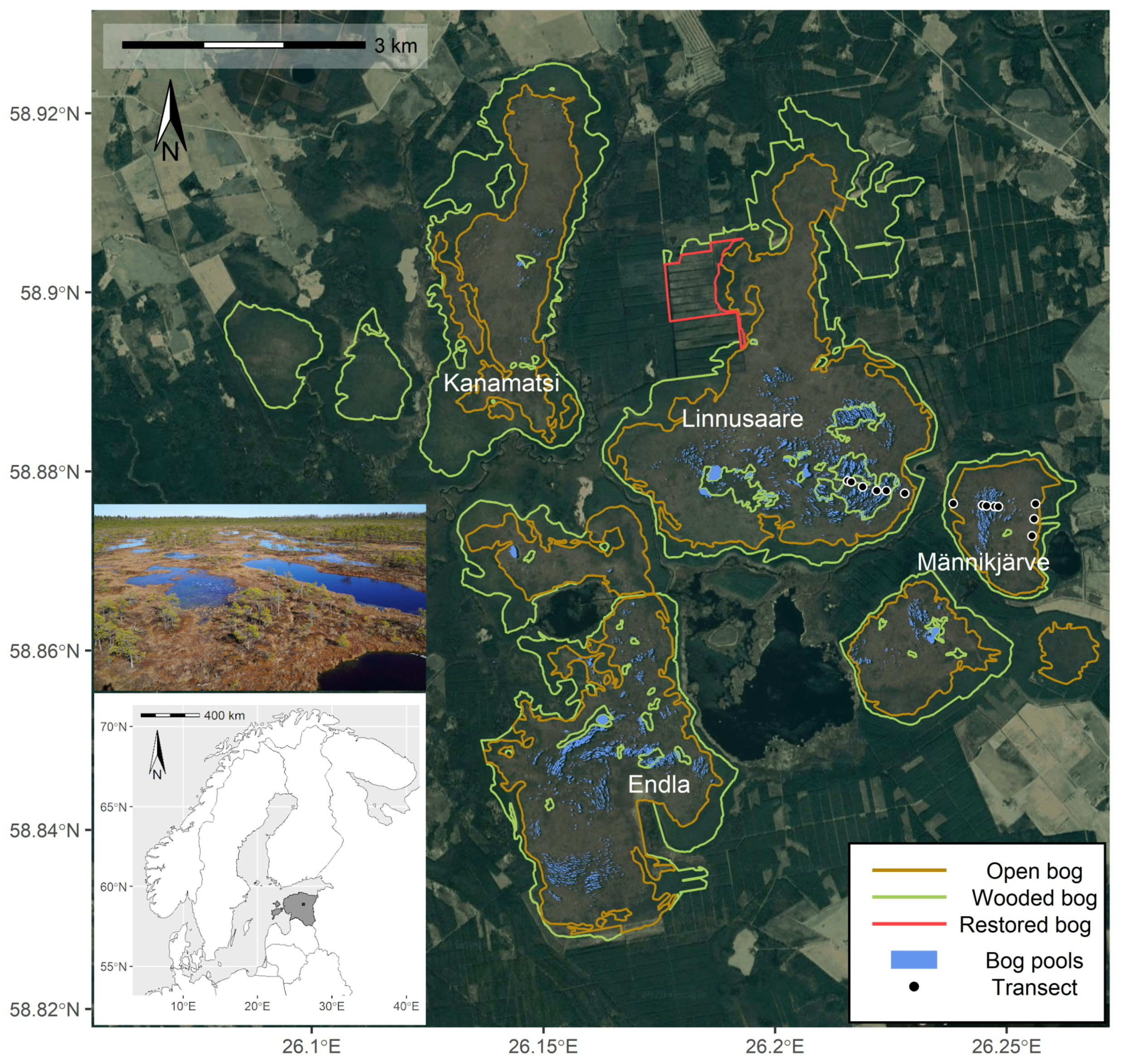
2.1. Study Area

Endla Nature Reserve (10,161 ha) is situated in central Estonia (58.88°N, 26.18°E). The reserve protects a diverse system of wetland habitats, the Endla mire complex and springs. Approximately half of the territory is covered by mires. The most prominent objects of the Endla Nature Reserve are the raised bogs, characteristic for northern temperate bogs. The largest bogs are Linnusaare (1250 ha), Endla (1100 ha) and Kanamatsi bog (690 ha), while smaller Männikjärve bog (208 ha) is located to the east of Linnusaare bog (Figure 1). The bogs are of limnogeneous origin with ecotopes of elongated ridges, pools, hummocks, lawns. and hollows microforms. The thickness of the peat is 3–6 meters, occasionally more than 7 m.
The open bogs are mainly Sphagnum-dominated ridge-hollow-hummock ecotopes, whereas in the central parts ridge-pool ecotopes are dominant with Pinus sylvestris trees (up to 5 m) growing abundantly on ridges between the pools. Marginal areas of bogs are wooded (Pinus sylvestris) or covered by bog forest (tree height 15–20 m) resulting mainly from drainage by the ditch network or surrounded by forest covered transitional bogs or fens.
Long term (1881–2018) mean annual air temperature at Tooma Mire Station is 4.5 °C. In February, the mean monthly air temperature is −6.8 °C and in July 16.8 °C. Monthly precipitation is unevenly distributed with minimum in winter and spring (<40 mm), maximum in summer and autumn (51–88 mm). The long term mean annual precipitation is 660 mm. Measured evapotranspiration during the vegetation period (May to October) in 2018 from bog and pool surface were 266.8 and 462.1 mm, respectively. Bog surface freezes normally in December and thaws in end of April [40].
The growing season spans from April to October. The bog water table is highest during snowmelt (April). Due to high discharges and evapotranspiration, the water table lowers rapidly in May and June, reaching the minimum level usually in July or August. In autumn precipitation induced pore water recharge increases the water table but it does not reach the spring maximum. In December the bog surface freezes and precipitation in the form of snow establishes snow cover. The frozen surface hinders infiltration of snowmelt water until the surface thaw in spring, causing secondary minimum in the water table in winter.

2.2. Water Table and Meteorological Data

The water table data were collected at Tooma Mire Station by the Estonian Environment Agency. The time series of Tooma Mire Station are collected on a routine basis along hydrological monitoring transects on Männikjärve bog since 1950 and the east–west transect was extended onto Linnusaare bog at the end of 1970. Water table is monitored automatically daily both by staff gauges in pools and sampling wells in peat, thus ensuring temporal concurrence to the SAR data. The sampling wells and staff gauges are anchored to the sediment underlying the peat layer. Water table is defined relative to the absolute surface height, corresponding to the average surface of the ecotope around the sampling well [40]. In this study, the average daily water table data from 24 October 2017 to 18 December 2018 were used and only the wells and staff gauges situating in the area classified as bog (open or wooded) were considered.
The meteorological data are provided by the Estonian Environment Agency. Meteorological observations were conducted from May to October at the meteorological station in the central part of Männikjärve bog and year-around at the main station on mineral soil located 1 km south-east. We used summarised daily precipitation value and air temperature measured at 6 p.m. local time, being closest to the SAR acquisition time, from the period of 24 October 2017 to 18 December 2018.

2.3. Land Cover Data

Peatlands have been distinguished based on Estonian Soil map (1:10,000) where all types of histosols were extracted with soil depth >30 cm. The land cover classification is based on the land cover maps from the Estonian Topographic Database provided in the Estonian Land Board Geoportal. The following land cover types were used: open bog, wooded bog, forest, and bog pools. The criteria for the open bog is tree height <1.3 m or canopy cover <0.3, wooded bog with tree height 1.3–10 m and canopy cover >0.3, forest with tree height >10 m and canopy cover >0.3, and bog pools with area >100 m2 were distinguished [41].

2.4. SAR Data

Our dataset comprises 18 Sentinel-1 (C-band) VV-polarization Interferometric Wide swath mode (IW) Single Look Complex (SLC) images acquired by satellite Sentinel-1A in ascending orbit (relative orbit number 160) covering 13 × 13 km2 in Endla mire complex from 24 October 2017 to 18 December 2018. The images were acquired with an incident angle about 39° and pixel spacing in range (rg) and azimuth (az) of 2.33 × 13.88 m and spatial resolution about 3.1 × 22.4 m (rg × az) in sub-swaths IW2 [42]. The acquisition time is around 15.56 UTC, corresponding roughly to 18.00 EET and 19.00 EEST (the Eastern European Summer Time being the local time for most of the acquisitions used in our study).
The dataset covers the growing season. Winter images from November 2017 to March 2018 are omitted because of the snow cover. The minimum and the maximum temporal baseline from the common master image of 28 May 2018 is 12 days and 216 days, respectively. The interferometric baselines vary between −82 and 106 m with respect to the common master image of 28 May 2018 (Table 1). VV data are used in the processing as the sensitivity to variations in soil moisture has been reported to be stronger in co-polarized mode, whereas vegetation volume scattering dominates in cross-polarization [43,44,45].

3. Methods

3.1. Coherence Estimation

We created 11 Differential Interferometric Synthetic Aperture Radar (DInSAR) [46] coherence image pairs which cover the growing season with roughly a monthly step. All the pairs are calculated from the single master image acquired on 28 May 2018 (no precipitation). The master image was chosen to ensure the highest InSAR coherence over the full stack while being as close as possible to the maximum water table after the snow melt in spring. Images before 28 May 2018 did not show sufficient coherence. After InSAR processing, the outputs were masked based on the land cover data and thereafter related to in situ water table data.
Coherence processing was executed with the European Space Agency’s (ESA) SNAP software version 6.0.0 [47]. The guidelines for Sentinel-1 TOPS DInSAR processing [48,49,50] were followed for coherence estimation in SNAP. The SNAP processing chain consisted of: S1 TOPS Coregistration with ESD, Coherence estimation (integrated with Topographic Phase Removal), TOPS Deburst and Range-Doppler Terrain Correction. SRTM 1 sec and bilinear interpolation were used for coregistration and terrain correction; the shifting window size for the coherence estimation is 3 in azimuth and 10 in range direction (3 × 10 pixels); no multi-looking was applied; EPSG:3301 (Estonian Coordinate System of 1997) was used.

3.2. DinSAR Processing

We used SARProZ software package [51] and Matlab for the conventional DInSAR processing to create 11 image pairs with the common master image from 28 May 2018. The analysis was performed in SAR slant range pixel coordinates in order to preserve phase values as much as possible. A 3 × 10 pixel window was used for coherence calculation, while for phase filtering with Goldstein filter [52] a larger 15 × 30 pixel filtering window was used. The interferograms were flattened with local Topographic Phase Removal, in order to present only LOS altitude differences. A temporal long term interferometric stack containing 11 date pairs over the growing season of 2018 was produced with reference to 28 May 2018. The stack contains, coherence amplitude images, interferometric phase images and unwrapped height difference images as well as masks for the open bog land cover type in SAR image coordinates.

3.3. Data Analysis

The InSAR coherence time series of the growing season were analyzed in R software (version 3.6.1) to identify spatio-temporal dynamics of coherence to identify factors (water level, land cover, precipitation, temperature) which affect decorrelation. The Shapiro–Wilk test was used to analyse data distribution, the Mann–Whitney U test (also known as the Wilcoxon rank-sum test) was used to compare samples, and the Spearman’s rank-order correlation was applied for not normally distributed data to evaluate correlation, and regression analysis to estimate relationship between variables were applied. All computed statistics were considered to be statistically significant if p value < 0.05. For non-linear regression model, Root Mean Squared Error (RMSE) was calculated.
In first stage, the open bog, wooded bog, bog pools and forest were extracted according to the land cover classification [41]. Subsequently, the pixels spatially corresponding to the sampling wells were extracted form InSAR coherence images and correlated with the water table measurements. Also, mean coherence of the open bog land cover class was related to the mean WT in the wells. WT dynamics have been reported to be relatively uniform in the open bog justifying modelling it as a unit [30,53]. Therefore, despite the availability of WT measurements from limited locations, we used their mean to represent the whole open bog area as separate time series of water measurements are strongly correlated ( ρ = 0.928–0.995, p < 0.05). The aggregation of pixels of a coherence image aims to represent the whole site [44] and to reduce the influence of randomness of individual pixel values [44,54]. Segmentation into objects has been advised for target objects much larger than one image pixel [54,55].
Thereafter, correlation and regression analysis were performed to examine the relationship between the time series of temporal coherence and the water table measurements and between coherence and meteorological data (air temperature, precipitation variations). Based on the coherence thresholds chosen according to our data and the literature [28,50,56], the spatial correlation between land cover and pixels of high coherence (≥0.5 and upper decile of the open bog pixels) and low coherence (≤0.25 and lower decile of the open bog pixels) was mapped. Also, the spatial DInSAR analysis was carried out. The unwrapped long term displacement maps were compared to land cover and water level data to evaluate capability of DInSAR to capture the bog breathing. Correlation and regression analysis ware used.

4. Results

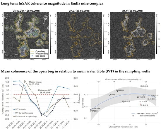
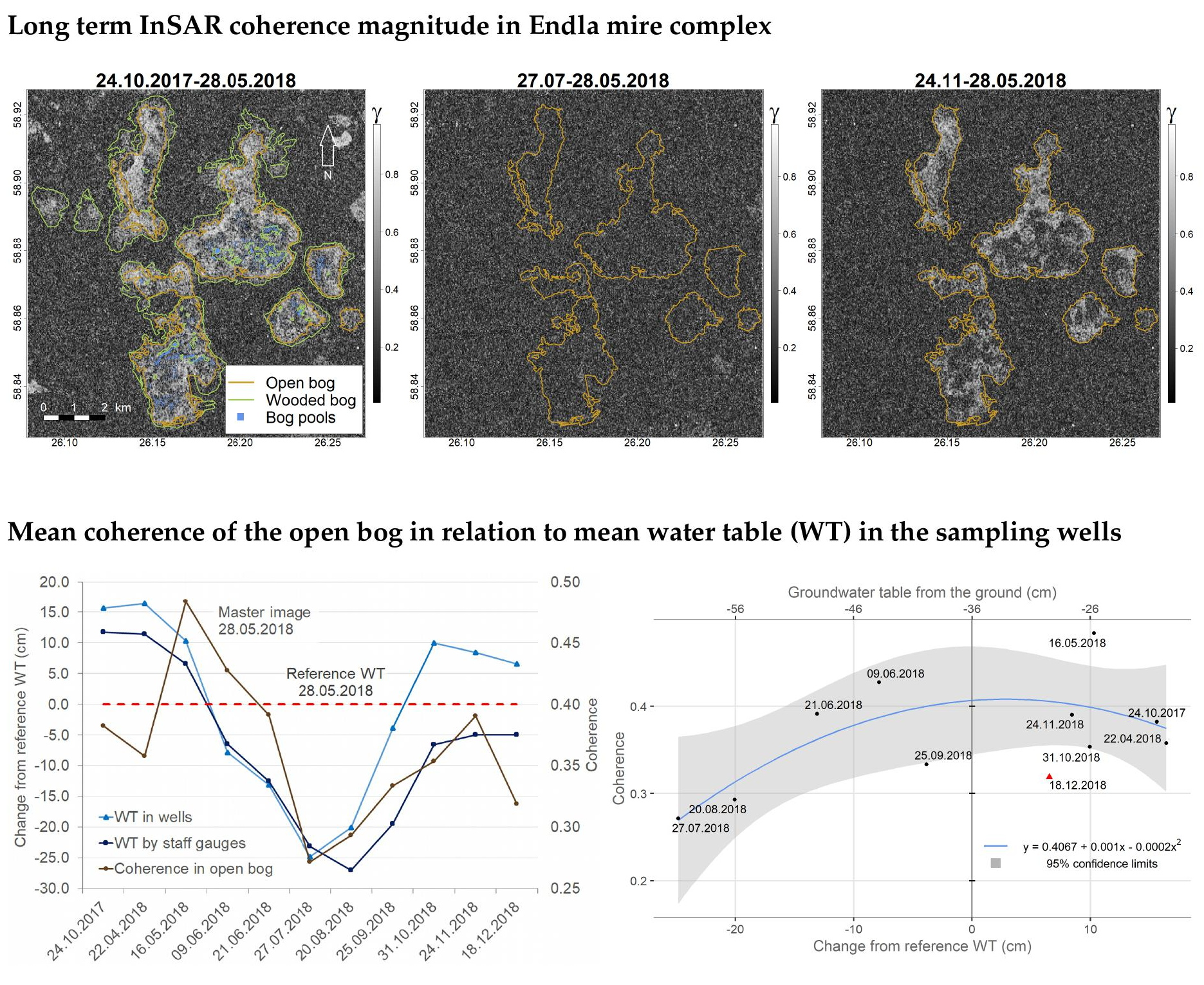
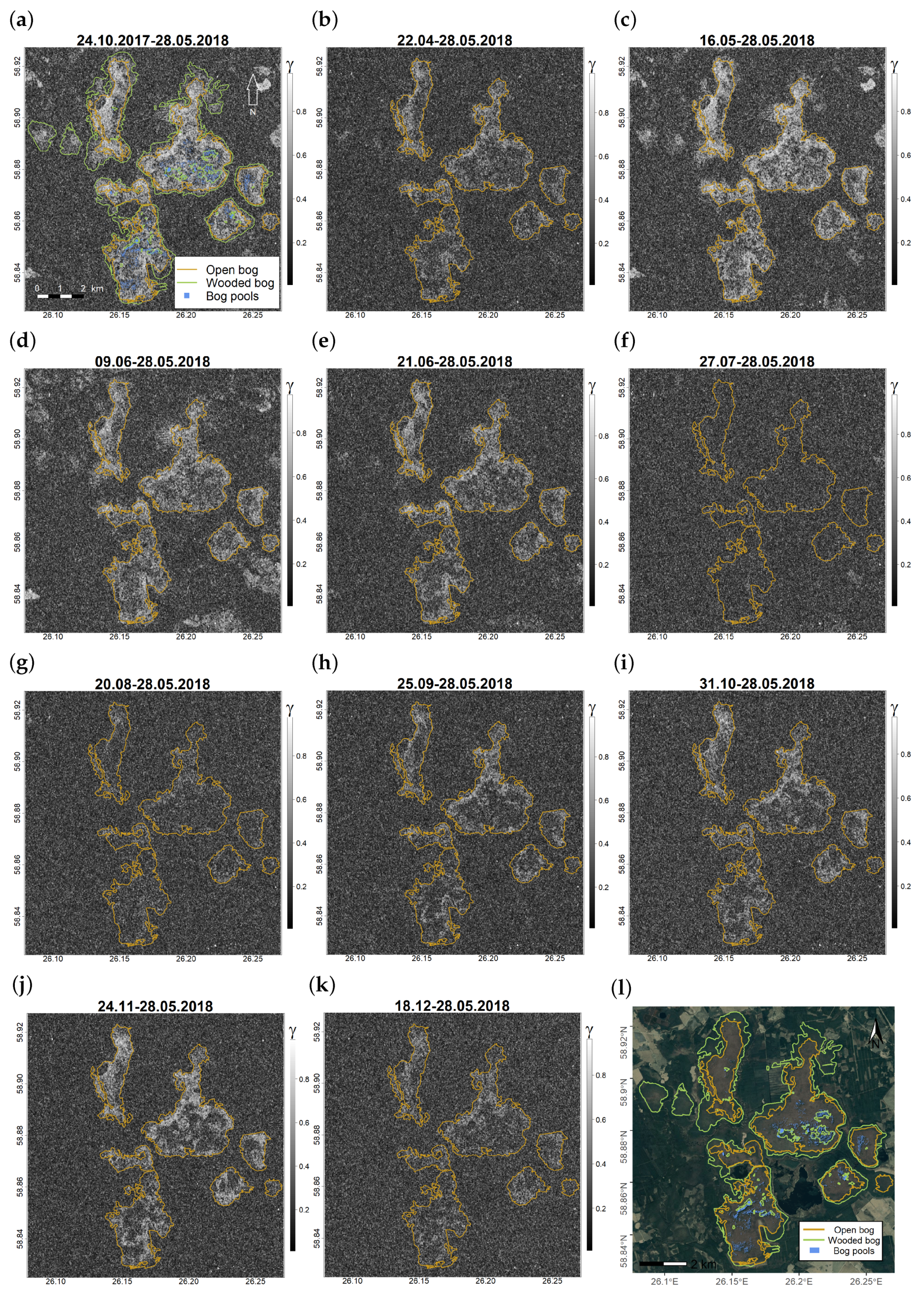
4.1. Seasonal InSAR Coherence in Endal Mire Complex

Our results show that the mean InSAR coherence of the open bog is significantly higher compared to other natural land cover classes (wooded bog, bog pools, forest) (p < 0.05) being the only element in landscape that is comparable to larger roads and built up areas in terms of retaining coherence. Also the bog pools and forest differ (p < 0.05). The wooded bog is statistically similar to bog pools and forest. The open raised bogs sustain coherence over the full growing season (snow free period from April to December 2018) and also over the winter (October 2017 to May 2018).
Moreover, the open bog display temporal variance in coherence—better correlated with the master image in the spring and the preceding and following autumn, while displaying low coherence in the summer, though the latter has shorter temporal baseline (Figure 2). All the open bogs in the Endla mire complex follow this dynamic and display the strongest average decorrelation in July when the water table is the lowest and backscatter therefore most affected by aeration of the peat layer. Precipitation and temperature might have effect on interferometric coherence (e.g., [57]). The reduction in coherence in December can be attributed to snowfall (total amount of precipitation water 5.4 and 1.0 mm) on 18 December and a day earlier, respectively. Other than that, the coherence does not display correlation to precipitation and the air temperature is not correlated either (Figure 3). The restored open bog site does not follow the pattern of coherence recovery characteristic to the natural open bog, probably due to the fact that the peatland restoration process e.g., damming ditches was still in progress in 2018 and water level dynamics was affected by different processes. Therefore this area is excluded from further analysis.
Any other natural land cover type do not display a comparable recovery in coherence as seen in Figure 4. The coherence of bog pools display only a slight recovery later in autumn. For the wooded bog, the lowest coherence values occur similarly to the bog pools in August and September and the coherence pattern may indicate slight signs of recovery in later autumn. The coherence of forested land fluctuates steadily around low values.

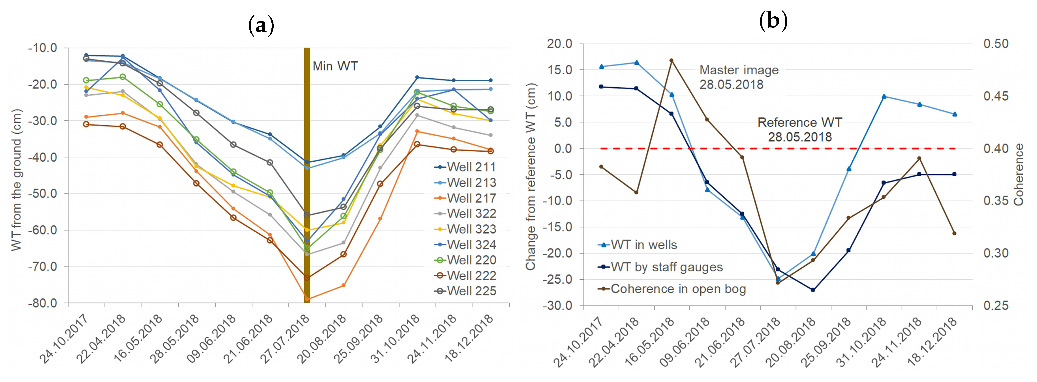
4.2. Seasonal Water Table Dynamics in Peat in Endla Mire Complex and Long Term Coherence

The water table recorded by sampling wells in peat and staff gauges in bog pools behave differently. The lowest WT in the wells in both Linnusaare and Männikjärve bog were observed with no exception in July (Figure 5a). Water level dynamics in all sampling wells were strongly correlated ( ρ = 0.928–0.995, p < 0.05), whereas in Linnusaare bog ρ is 0.958–0.975 and in Männikjärve ρ is 0.928–0.986. Nevertheless, the magnitude of the WT dynamics relative to bog surface is different in sampling wells (observed WT between 12 and 79 cm below the ground, corresponding to the seasonal water level range of 29–51 cm). The water table in bog pools measured by staff gauges located in central parts of bog experienced seasonal change in WT in range of 36–43 cm (correlation ρ = 0.861–0.994). The lowest WT measured by the staff gauges in the pools occur in August when the WT in the sampling wells in peat have already turned to rise (Figure 5b). The phenomenon of staff gauges lagging behind wells is partly related to relatively large quantity of of non- or less-transpiring biomass (litter, reduced transpiration from trees, Vaccinum and Ericaceae sheltering the ground) in second half of the summer sheltering the ground, resulting in higher resistance to evaporation compared to the open surface of pools [58,59]. Also, in July when the water table in the wells is the lowest, the mean coherence of the open bog area (calculated relative to a single master image of 28 May 2018) is the lowest as well. The larger is the difference form from the reference water level (corresponding to the day of the master image, 28 May 2018) the lower is the coherence.
However, correlating the water level in sampling wells directly to coherence of the corresponding pixel does not display clearly correlated pattern. Even if the coherent-most nearby pixel (let it be called adjusted well pixel) is chosen instead, patterns are not related between the coherence time series of the individual pixel and water table in the corresponding well in this spatial scale. The decorrelation results from variances in micro relief and size of microtopes several times less than the pixel size, vicinity of pools or presence of trees which causes randomness at a single pixel level. Though, by averaging all the pixels extracted as described (coherent-most nearby pixels to the wells and thus representing ecotope), the correlation appears to follow again the same dynamics as simple averaging over the whole open bog does (Figure 6a). The correlation between the time series of mean coherence in the open bog and the mean coherence of the adjusted well pixels is 0.845 (p < 0.05), correlation between the coherence of open bog and the well pixels is 0.745 and 0.682 between well pixels and adjusted well pixels.
The second degree polynomial regression model (Figure 6b) describes the relationship between the coherence and water table (RMSE = 0.041 for | γ | ). Coherence of 18 December 2018 is omitted from calculation of regression as an outlier because its low coherence value is due to two consecutive days of snowfall. The WT changes above the reference water level (28 May 2018) relate to higher coherence values compared to WT changes below the reference, as the image pair of 16 May–28 May displays higher coherence than 9 June–28 May despite having larger WT difference at equal temporal baseline. Similarly, 25 September displays lower coherence compared to 31 October though the difference from the reference WT is notably smaller for the image in September (Figure 5b). This indicates that the direction of the water table change may be important to be considered and a linear regression model may not be applicable. Alternatively, if to presume the direction of the change is not important and both increase and decrease in soil moisture produces the same coherence loss [36], the linear model with the absolute values of water table difference could be meaningful ( R 2 = 0.333, p = 0.081).

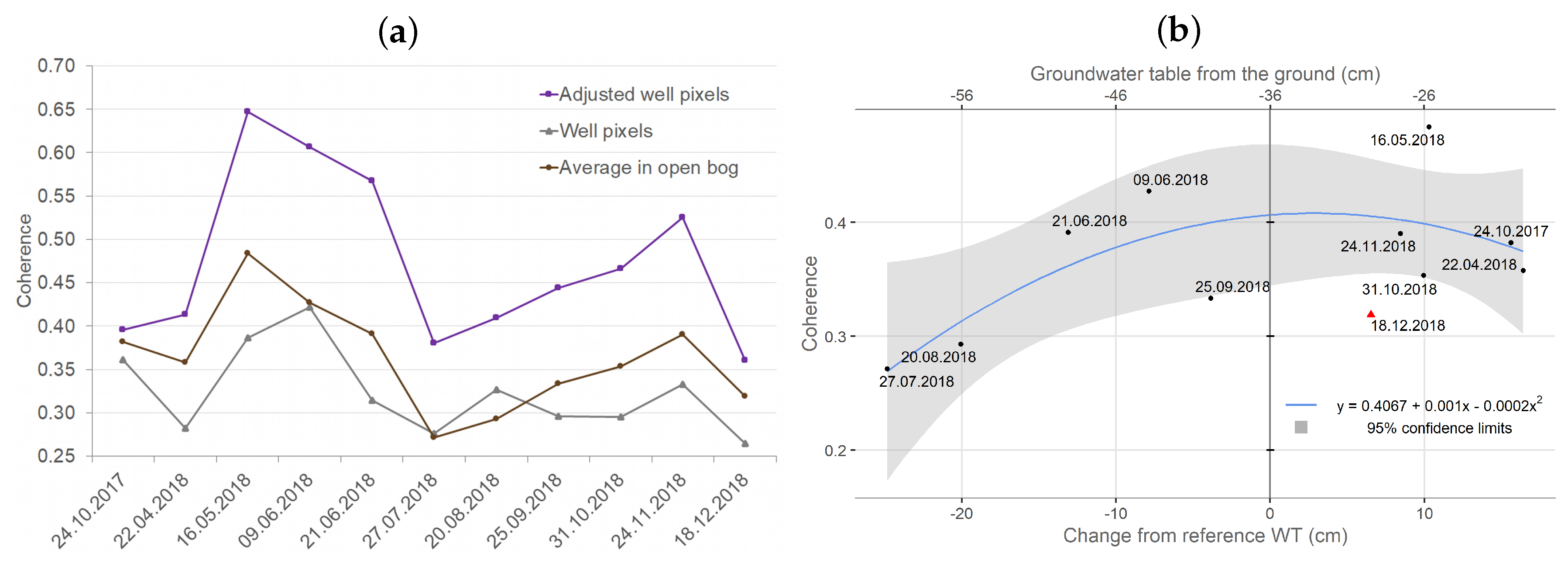
4.3. Spatial Dynamics of Long Term Coherence for Areas of High and Low Coherence

Masking in only the pixels of higher mean coherence ( | γ | ≥ 0.5 threshold set according to our data and the literature [28,50,56]; upper 10% percentile of the open bog pixels) reduces the number of pixels containing backscatter from trees or neighbouring pools (pools themselves are masked out by default). The pixels of higher mean coherence are concentrated to the most homogeneous hummocks dominated ecotope with low micro relief and no pools and hollows (Figure 7). In central parts of the bogs the highest coherence is observed for regions dominated by hummocks and lawns, only occasionally in areas dominated by extensive hollows. The temporal dynamics of pixels of higher mean coherence and the dynamics of averaged coherence of the open bog are strongly correlated (0.900, p < 0.05). The lowest coherence ( | γ | ≤ 0.25; lower 10% percentile of the open bog pixels) occurs in the vicinity of pools and ridge areas with higher tree canopy cover in central parts of the bogs and in bog margins close to the wooded bog or peatland forests (Figure 7). The temporal dynamics of pixels of lower mean coherence and the dynamics of averaged coherence of the open bog are strongly correlated (0.873, p < 0.05). Correlation between the dynamics of pixels of lower and higher mean coherence is 0.736 (p < 0.05).
In addition, we experimented with only those pixels which remain coherent over a given threshold value in each image. Although the open bog area does not contain any persistent scatterers as there are no pixels with a value over 0.65 through all images in period 24 October 2017–18 December 2018, there are only 62 pixels in the open bog land cover class maintaining coherence over 0.5 in each of the images of the full stack. Nevertheless, the results from such extraction of the open bog pixels which maintain coherence over 0.5 in every image of the stack follow the temporal dynamics of coherence change similar to method of simply averaging pixels value over the open bog land cover class (correlation 0.891, p < 0.05). However, such a reduction of available pixels for analysis is a notable undesirable aspect of strict coherence-based thresholding.

4.4. DInSAR Phase Measurements over the Open Bog

As previously shown, SAR images stay coherent over open bog areas for over half a year. This allows deriving the phase differences by using DInSAR technique, allowing potential high accuracy estimation of bog surface vertical movements, so-called bog breathing. The DInSAR phase errors introduced by atmosphere are still a known limitation though in most weather conditions the atmosphere induced errors should stay relatively constant over a few kilometers [60,61,62]. On the other hand, the surface of the bog cannot move arbitrarily. Thus, the possible displacement shall always be moderate and continuous, as the bog surface is always continuous. Following those assumptions, phase unwrapping can be performed locally in smaller area and displacement estimates can be derived. Another challenge for DInSAR phase estimation is the low signal and low coherence for open water areas (bog pools) and trees. Considering the above mentioned factor, we used coherence weighted phase filtering (Goldstein Phase Filtering [52]), unwrapped the phase and calculated DInSAR displacement maps over the growing season (snow free period May 2018 to November 2018) as shown in Figure 8.
The reduction of coherence in summer months caused by lower water table, further amplified by presence of bog pools and ridge areas with higher tree canopy cover are noticeable, especially in August when the phase map is the noisiest and cannot be relied upon. The DInSAR performed best locally in bogs without open water and ridge areas with higher tree canopy cover, such as Kanamatsi bog. Displacement maps reveal membrane-like dynamics for the bog surface, where the central area of the bog surface has larger elevation changes (deformations up to 2 cm relative to the tie-point used) while the border areas have smaller changes. This is in good agreement with the structure of the bogs and expected bog surface vertical movement due to changing water content in porous peat matrix in the middle part of the raised bog [63,64,65]. DinSAR phase image can have biases over larger area and therefore absolute height difference is difficult to be measured. However, for smaller areas it can be assumed that some areas are not moving and movement can be locally calibrated.
Based on our preliminary results (Figure 8), it can be concluded that DInSAR is able to capture seasonal peat surface dynamics in open bogs while the other land cover classes do not maintain sufficient coherence for successful implementation of the method. To analyse the vertical dynamics of the peat surface, we studied the vertical bog surface profile along a cross-section of Kanamatsi bog. Kanamatsi bog is chosen for method demonstration due to its smallest concentration of bog pools reducing InSAR coherence. The bog pools and tree growth in surrounding ridges cause phase decorrelation and discontinuities in otherwise continuous reliable phase surface of the open bog area. To avoid or keep as low as possible such discontinuities and to form a uniform field for phase reconstruction we selected an open bog best suitable for DInSAR from the area. The Kanamatsi bog has the most homogeneous land cover (hummocks dominated ecotope) and few pools compared to the other bogs in the mire complex. Only in Kanamatsi bog, being almost without trees and pools, a continuous reliable phase surface formed also in middle parts of the bog, which could be related to a tie point. Despite the water table has not been measured in Kanamatsi the average WT from nearby Linnusaare and Männikjärve bogs can be used for comparison, and as shown in Figure 8 the general seasonal pattern of the vertical displacement in Kanamatsi is in good accordance with these bogs. Figure 9a shows the profile and the DInSAR displacement map for Kanamatsi bog in September. Bog surface elevation change profiles were extracted from all displacement images from period 16 May 2018–24 November 2018 (Figure 9b). The atmospheric effects were accounted for by a simplified approach of using a tie-point from the profile which was assumed to be the zero displacement in all the images. This tie-point is taken from the bog margin where peat layer is shallow and bulk density high, tree growth already occurs and which is away from dynamic area in the middle of the bog with thick layer of porous water filled peat with low bulk density. Using such a local tie point, the displacement profiles from different image pairs can be bundled and simple comparison with water level changes can be made. Regarding the direction and amplitude of the displacement, the DInSAR image stack with single master is internally coherent. The displacements (calculated independently for every image pair) agree in general terms with each other (Figure 9b). Exception here is 8 August which had the lowest water table in the sampling wells out of all the SAR acquisition dates we processed and when the coherence was so low that it was not possible to derive reliable phase estimate.
To visualise the bog surface height seasonal dynamics, we chose a point on the profile and show the displacement as a single point time series in Figure 10a related to the mean water level change from the sampling wells (Figure 10b). The relationship is described by the linear regression model ( R 2 = 0.59; the image pair of 28 May–8 August as an outlier omitted). The result is indicative as it depends on tie-point and transect placement. However, the behavior of displacement of the point in general agrees with the expected bog breathing which follows the dynamics in water table, showing surface subsidence in the centre of bog for dry summer and uplift in autumn when peat pores recharge with rain water. August, because of its low phase correlation can be considered to be an outlier. The figure indicates also that the range of phase center dynamics on the peat surface is only in magnitude of one tenth of the water level change. Kanamatsi bog with its consistent displacement pattern over entire season (decorrelated August excluded) suggests that the observed displacement is real.

5. Discussion

Our results show sustained interferometric coherence and capability for DInSAR phase measurements in open raised bogs over more than half a year. This is in accordance with some previous research [25,39] while other studies have reported the loss of coherence in peatlands, including the open bog, assigned to vegetation growth [26] resulting in gradually decreasing average coherence over time [23,24]. However, the Sphagnum and low shrubs dominated vegetation in the open raised bog is temporarily homogeneous, constituting of insignificant seasonal herbaceous growth or deciduous vegetation. Seasonal herbaceous growth could have significant impact on coherence merely in the vicinity of drainage ditches associated to the lowered water table in peat and in fens. The effect of the drainage becomes minimal in 80 m from the ditch [30] but may extend further depending on the type of drainage [66] and mire type [53]. That corresponds to around 6 pixels in our case (14 × 14 m ground resolution). However, ditch affected areas are also the areas of advanced tree growth [67,68], thus being generally masked out as the wooded bog in our study.
We also demonstrated that besides sustaining InSAR coherence over a longer time period, there is a temporal variance in coherence over the open bog. To the best of our knowledge, such a recovery of long term temporal coherence in natural vegetated landscapes, except form decorrelation caused by snow cover or due to temporal inundation (for example [33,69]), has not been shown previously. The return of short term temporal coherence (with respect to a single master image) to higher values has been reported in agricultural fields where soil moisture and coherence displayed similar temporal behaviour [70]. However, we showed the variable nature of long term coherence in the peatland to be following the water table dynamics. Previously, the close relationship between changes in SAR backscatter intensity σ 0 and ground water table in peatlands has been demonstrated [32,34,35]. Herewith, Kasischke et al. [71] found the correlation of σ 0 to groundwater depth existed only in open fens but not in a forested fen, which is in accordance with our results for the bog. Also, the phase changes have been tried to be related to peatland ground water table dynamics [32]. Nevertheless, the approach of relating WT in peat through consequent soil moisture content [30,34] to coherence is novel. In general, interferometric coherence is known to be influenced by temporal decorrelation, volumetric decorrelation, ground changes and soil moisture, rising a legitimate doubt about possibility of direct quantification of the soil moisture from the coherence [72]. However, due to the stable nature of the vegetation in the open bog, we consider such a study worth to be undertaken and the results, whether quantitative or qualitative, are possibly beneficial for monitoring seasonal dynamics of water content in bogs could improve models of GHG exchange in peatland soil-atmosphere system.
The different methods we tested in this study to relate peat WT dynamics to InSAR coherence over a landscape scale gave comparable results, hence the simplest model of averaging coherence of all the pixels in domain could be optimal. The open bog land cover mask, if not available from a predefined land cover classification, could be derived from ancillary remote sensing sources [73,74] or, based on the findings of this paper, the InSAR coherence could be used for discrimination. Despite demonstrating the correlation between coherence and the peat WT dynamics in the open bog, we did not find it to be linear. That may indicate slow temporal decorrelation and importance of direction of water table change over the mere absolute value of change as peat moisture reacts differently during pore water discharge and recharge, in regard to coherence retention. Nevertheless, the images from late autumn (31 October, 24 November) with WT notably higher than the reference (28 May 2018) show better correlation than 25 September image with only slightly lower WT than the reference, while the latter has also a shorter temporal baseline. Also, the image pairs with 28 May 2018 as master image display higher coherence values than comparable pairs with 16 May or 9 June as master despite the latter have smaller WT difference (9 June–25 September; 16 May–31 October; 16 May–24 November). All that indicates that in regard to coherence retention, more important than the sole WT change (relative to the reference WT of master image) could be the initial WT depth of the chosen master image or the initial soil moisture. Accordingly, the soil moisture model for bare agricultural lands by De Zan et al. [36] showed the magnitude of coherence and phase changes to depend on the image taken as a reference. However, further analysis is required to identify factors related to choosing the optimal master image.
SAR mostly does not receive backscatter directly from the ground water table but records soil humidity that has a close relationship to WT [32,35]. The relationship for backscatter intensity σ 0 in peatlands has been found to be weaker or partly disappearing in summer, possibly in relation to the reduced capillary water rise at deeper water table [35]. Furthermore, peat acts differently depending on whether the water content is decreasing or increasing [65]. Firstly, the bog surface tends to be higher when drying out (spring and summer) and lower when pores are recharging (in autumn) at the comparable peat water table [65]. However, coherence magnitude is insensitive to displacements [75]. Secondly, when the water saturated peat dries, pores are filled with air but when pore water recharge happens in autumn and the water table is restored, some pores stay filled with air [76]. The lower soil moisture content causes lower dielectric constant [44,77] which in turn results in weaker σ 0 [38,78] and deeper vertical propagation of the radar signal into the soil [36,78,79]. Soil moisture induced changes in signal penetration depth up to 60 mm have been shown for C-band SAR [80]. Nevertheless, changes merely in penetration depth do not contribute to the phase changes but only to coherence loss [36]. However, no quantitative research of SAR penetration into peat is so far available [44].
The moisture-dependency of phase changes and coherence loss [81] were shown to be linked to soil moisture content in agricultural lands [36,82,83], whereas if vegetation is present the water status of plants also contributes [72,84]. Furthermore, as decrease in soil moisture causes a decrease in the optical path to the sensor [85], during dry summer months the real surface subsidence may be masked by spurious drying-induced uplift corresponding to 20–30% of the radar wavelength [70,75]. The latter could partly explain why the summer image pairs show smaller displacement than the 28 May–13 September image pair in the single point time series form Kanamatsi bog. It could also contribute to explanation why 28 May–8 August, which corresponds to the lowest average WT, performs as an outlier among bog surface profile and in the single point time series. In our test site, the WT in peat fluctuated between 12–79 cm below the surface, indicating the potential of both bog breathing and differences in humidity, possibly to contribute to the dynamics of phase changes. However, as we do not possess in situ data of peat surface oscillation, our study cannot neither reveal the accuracy of displacement estimation nor the magnitude of contribution from soil moisture to phase changes obtained by the DInSAR method.
Reliable phase measurements for estimating seasonal oscillation of peat surface (or WT table dynamics in peat) in northern raised bogs have not been demonstrated previously. The seasonal surface oscillations in magnitude of up to ∼2 cm presented by Zhou et al. [24], using Stanford Method for Persistent Scatterers (StaMPS) [86] were encouraging, though not validated with in situ measurements and showing disparity between ascending and descending orbits. However, Rawlins et al. [27] demonstrated the usability of Intermittent Small Baseline Subset (ISBAS) technique [87] for long-term peatland deformation monitoring, Cigna et al. [28] concluded with the need for further research to also gain reliable non-linear deformation results with ISBAS. Kim et al. [32], using the Small Baseline Subset (SBAS) technique [88,89], did not succeed in phase unwrapping in the low vegetated shrub land in the Great Dismal Swamp, though they associated the phase changes with the groundwater table induced changes in soil moisture.
The DInSAR of our study produced promising preliminary results as we recorded displacement dynamics up to 3 cm for Kanamatsi bog. A disadvantage is that we do not have in situ surface oscillation measurements to compare with in this particular bog. However, if to speculate that the phase actually did gauge the bog surface oscillation, the DInSAR results may be realistic in regard to the WT data (average range of seasonal WT change 42 cm) and what is know of bog breathing in other sites. The bog breathing has been shown to normally constitute 2.6–11 cm [65,66,90]. Oscillation is know to be largest in sites with shallowest water table, whereas drier sites suggest loss of elasticity [65]. Geographically close Umbusi bog in central Estonia had measured surface oscillation in the range of ∼5 cm in 2015 and 2016 [66]. Thus, our relatively small range of vertical surface oscillation, up to 3 cm relative to the tie-point we used, recorded in Kanamatsi profile could rather be an underestimate, while the narrow oval shape of the bog could indeed contribute to smaller surface oscillation. In other bogs in the Endla mire complex, more circular and domed in shape, the magnitude of seasonal surface deformations the DInSAR recorded could also be underestimated. The recorded modest deformation values have to be attributed partly to the shading effect of the forest. The possible tie-points for unwrapping (where no deformation occurs) lie on the border of the bog where stable mineral land occurs. These tie-points and the adjacent peatland area are normally covered by forest and stay shaded by canopy, being decorrelated and therefore not suitable for reliable phase estimates with C-band InSAR. Hence, for reliable deformation results tie-points should be located at open peatland area with shallow organic soil or at mineral soil adjacent to the open bog. First promising results with DInSAR derived bog surface displacements and its consistent behaviour through the vegetation period signify the potential of the method. Perspective of monitoring bog surface oscillation as a metric for assessing the capacity of water storage in bogs or restoration success [65] with InSAR encourages further research [24]. Further validation of DInSAR method could be carried out over an area with existing in situ oscillation measurements and a stable (or known) tie-point.

6. Conclusions

Understanding seasonal dynamics of peatland surface and volume, often referred to as bog breathing, and spatial dynamics of WT are key to improving spatial models of material flow at landscape level. The objective of this study was to examine the applicability of Sentinel-1 Interferometry (InSAR) to characterize seasonal dynamics of peatland surface and water table (WT) in peat over open raised bog areas in Endla mire complex in central Estonia, characteristic for northern temperate bogs. Our dataset comprised 18 Sentinel-1 (C-band) Interferometric Wide swath mode (IW) Single Look Complex (SLC) VV-polarized images acquired by satellite Sentinel-1A in ascending orbit (relative orbit number 160) from 24 October 2017 to 18 December 2018. The dataset covered the growing season. Two small baseline InSAR stacks of 11 image pairs related to a common master image (28 May 2018) were computed, respectively for estimation of coherence magnitude and surface deformation. Correlation and regression analysis were performed to examine the relationship between the time series of temporal coherence and the WT measurements and meteorological data in the open bog. DInSAR analysis was carried out to identify the surface deformation over the season.
Our results show that relatively high interferometric temporal coherence, sufficient for differential interferometric (DInSAR) analysis, was preserved in open bogs with temporal baseline over six months. The magnitude of the coherence was related to peat WT dynamics. While the coherence decreased steadily through spring and summer when WT was dropping, it made a recovery in autumn when the WT re-achieved the spring level. The relationship between mean WT and coherence averaged over the entire open bog can be described by second degree polynomial regression model (Root Mean Squared Error RMSE = 0.041 for | γ | ). It was found that more important than sole ground water table change relative to the reference WT of master image could be the initial peat WT depth of the chosen master image reflecting the initial soil moisture content and peat properties determining the pore water discharge and recharge. However, further work on understanding the mechanism for master image selection is needed. Inside the open bog, the pixels of higher coherence are concentrated to the most homogeneous hummocks dominated ecotope, while the lowest coherence occurs in the vicinity of pools and ridge areas with higher tree canopy cover and in bog margins close to the wooded bog or peatland forests. DInSAR analysis indicates seasonal bog oscillation and differences between bogs and for ecotopes within a bog. The relationship between surface oscillation and mean WT is described by linear regression model (Root Mean Squared Error R 2 = 0.59) in Kanamatsi bog. However, our analysis did not eliminate atmospheric effects on phase, and in situ levelling data are also required to calibrate DInSAR estimates locally.
Our findings suggest that the InSAR long term temporal coherence could be used to describe seasonal ground water table dynamics in open bogs during vegetation periods and differentiate between mire types and ecotopes. We also conclude that DInSAR analysis has the potential to gauge seasonal vertical bog surface movements and volume change, due to sufficient long term coherence between SAR scenes. Further development of the DInSAR-based application should be undertaken in locations where the ground water table and soil humidity measurements and bog surface oscillation data are available. Also a improved temporal resolution is required to reveal details of the dynamics.

Author Contributions

Conceptualization, T.T., J.P. and A.K.; methodology, T.T., J.P., A.K. and R.U.; formal analysis, T.T. and J.P.; resources, A.K.; writing–original draft preparation, T.T.; writing–review and editing, J.P. and A.K.; supervision J.P., A.K. and R.U. All authors have read and agreed to the published version of the manuscript.

Funding

This study is part of the PhD research supported by the European Union from the European Regional Development Fund (ERDF). Also, the study was financially supported by the ERDF within “National Programme for Addressing Socio-Economic Challenges through R&D (RITA)”, Estonian Research Council grant PRG352 and State Forest Management Centre grant LLTOM17250.

Acknowledgments

The authors would like to thank Anto Aasa (University of Tartu) for helping with R, and also Datel AS (Estonia) and Juhan-Peep Ernits (Tallinn University of Technology) for providing computing capacity.

Conflicts of Interest

The authors declare no conflict of interest. The funders had no role in the design of the study; in the collection, analyses, or interpretation of data; in the writing of the manuscript, or in the decision to publish the results.

References

  1. Gorham, E. Northern Peatlands: Role in the Carbon Cycle and Probable Responses to Climatic Warming. Ecol. Appl. 1991, 1, 182–195. [Google Scholar] [CrossRef] [PubMed]
  2. Yu, Z.; Loisel, J.; Brosseau, D.P.; Beilman, D.W.; Hunt, S.J. Global peatland dynamics since the Last Glacial Maximum. Geophys. Res. Lett. 2010, 37. [Google Scholar] [CrossRef]
  3. Köchy, M.; Hiederer, R.; Freibauer, A. Global distribution of soil organic carbon—Part 1: Masses and frequency distributions of SOC stocks for the tropics, permafrost regions, wetlands, and the world. SOIL 2015, 1, 351–365. [Google Scholar] [CrossRef] [Green Version]
  4. Leifeld, J.; Menichetti, L. The underappreciated potential of peatlands in global climate change mitigation strategies. Nat. Commun. 2018, 9, 1–7. [Google Scholar] [CrossRef] [Green Version]
  5. Drösler, M.; Freibauer, A.; Christensen, T.R.; Friborg, T. Observations and Status of Peatland Greenhouse Gas Emissions in Europe. In The Continental-Scale Greenhouse Gas Balance of Europe; Dolman, A.J., Valentini, R., Freibauer, A., Eds.; Ecological Studies; Springer: New York, NY, USA, 2008; pp. 243–261. [Google Scholar] [CrossRef]
  6. Parish, F.; Sirin, A.; Charman, D.; Joosten, H.; Minayeva, T.; Silvius, M.; Stringer, L. (Eds.) Assessment on Peatlands, Biodiversity and Climate Change: Main Report; Global Environment Centre, Kuala Lumpur and Wetlands International: Wageningen, The Netherlands, 2008. [Google Scholar]
  7. Ojanen, P.; Minkkinen, K.; Alm, J.; Penttilä, T. Soil–atmosphere CO2, CH4 and N2O fluxes in boreal forestry-drained peatlands. For. Ecol. Manag. 2010, 260, 411–421. [Google Scholar] [CrossRef]
  8. Yu, Z.C. Northern peatland carbon stocks and dynamics: A review. Biogeosciences 2012, 9, 4071–4085. [Google Scholar] [CrossRef] [Green Version]
  9. Webster, K.L.; Bhatti, J.S.; Thompson, D.K.; Nelson, S.A.; Shaw, C.H.; Bona, K.A.; Hayne, S.L.; Kurz, W.A. Spatially-integrated estimates of net ecosystem exchange and methane fluxes from Canadian peatlands. Carbon Balance Manag. 2018, 13, 16. [Google Scholar] [CrossRef]
  10. Joosten, H.; Tapio-Biström, M.L.; Tol, S. (Eds.) Peatlands: Guidance for Climate Change Mitigation through Conservation, Rehabilitation and Sustainable Use, 2nd ed.; Food and Agriculture Organization of the United Nations and Wetlands International: Rome, Italy, 2012. [Google Scholar]
  11. Chapman, S.; Buttler, A.; Francez, A.J.; Laggoun-Défarge, F.; Vasander, H.; Schloter, M.; Combe, J.; Grosvernier, P.; Harms, H.; Epron, D.; et al. Exploitation of Northern Peatlands and Biodiversity Maintenance: A Conflict between Economy and Ecology. Front. Ecol. Environ. 2003, 1, 525–532. [Google Scholar] [CrossRef]
  12. Tuukkanen, T.; Marttila, H.; Kløve, B. Predicting organic matter, nitrogen, and phosphorus concentrations in runoff from peat extraction sites using partial least squares regression. Water Resour. Res. 2017, 53, 5860–5876. [Google Scholar] [CrossRef]
  13. Waddington, J.M.; Morris, P.J.; Kettridge, N.; Granath, G.; Thompson, D.K.; Moore, P.A. Hydrological feedbacks in northern peatlands. Ecohydrology 2015, 8, 113–127. [Google Scholar] [CrossRef]
  14. Lees, K.; Quaife, T.; Artz, R.; Khomik, M.; Clark, J. Potential for using remote sensing to estimate carbon fluxes across northern peatlands—A review. Sci. Total Environ. 2018, 615, 857–874. [Google Scholar] [CrossRef] [PubMed]
  15. Jones, K.; Lanthier, Y.; van der Voet, P.; van Valkengoed, E.; Taylor, D.; Fernández-Prieto, D. Monitoring and assessment of wetlands using Earth Observation: The GlobWetland project. J. Environ. Manag. 2009, 90, 2154–2169. [Google Scholar] [CrossRef]
  16. Torbick, N.; Persson, A.; Olefeldt, D.; Frolking, S.; Salas, W.; Hagen, S.; Crill, P.; Li, C. High Resolution Mapping of Peatland Hydroperiod at a High-Latitude Swedish Mire. Remote Sens. 2012, 4, 1974–1994. [Google Scholar] [CrossRef] [Green Version]
  17. Merchant, M.A.; Adams, J.R.; Berg, A.A.; Baltzer, J.L.; Quinton, W.L.; Chasmer, L.E. Contributions of C-Band SAR Data and Polarimetric Decompositions to Subarctic Boreal Peatland Mapping. IEEE J. Sel. Top. Appl. Earth Obs. Remote Sens. 2017, 10, 1467–1482. [Google Scholar] [CrossRef]
  18. Canisius, F.; Brisco, B.; Murnaghan, K.; Van Der Kooij, M.; Keizer, E. SAR Backscatter and InSAR Coherence for Monitoring Wetland Extent, Flood Pulse and Vegetation: A Study of the Amazon Lowland. Remote Sens. 2019, 11, 720. [Google Scholar] [CrossRef] [Green Version]
  19. Hu, J.; Li, Z.W.; Ding, X.L.; Zhu, J.J.; Zhang, L.; Sun, Q. Resolving three-dimensional surface displacements from InSAR measurements: A review. Earth Sci. Rev. 2014, 133, 1–17. [Google Scholar] [CrossRef]
  20. Osmanoğlu, B.; Sunar, F.; Wdowinski, S.; Cabral-Cano, E. Time series analysis of InSAR data: Methods and trends. ISPRS J. Photogramm. Remote Sens. 2016, 115, 90–102. [Google Scholar] [CrossRef]
  21. Crosetto, M.; Monserrat, O.; Cuevas-González, M.; Devanthéry, N.; Crippa, B. Persistent Scatterer Interferometry: A review. ISPRS J. Photogramm. Remote Sens. 2016, 115, 78–89. [Google Scholar] [CrossRef] [Green Version]
  22. Bourgeau-Chavez, L.L.; Endres, S.L.; Graham, J.A.; Hribljan, J.A.; Chimner, R.A.; Lillieskov, E.A.; Battaglia, M.J. 6.04—Mapping Peatlands in Boreal and Tropical Ecoregions. In Comprehensive Remote Sensing; Liang, S., Ed.; Elsevier: Oxford, UK, 2018; pp. 24–44. [Google Scholar] [CrossRef]
  23. Zhou, Z. The Applications of InSAR Time Series Analysis for Monitoring Long-Term Surface Change in Peatlands. Ph.D. Thesis, University of Glasgow, Glasgow, UK, 2013. [Google Scholar]
  24. Zhou, Z.; Waldron, S.; Li, Z. Integration of PS-InSAR and GPS for monitoring seasonal and long-term peatland surface fluctuations. In Proceedings of the Remote Sensing and Photogrammetry Society Conference Remote Sensing and the Carbon Cycle, London, UK, 5 May 2010; Volume 1. [Google Scholar]
  25. Alshammari, L.; Large, D.; Boyd, D.; Sowter, A.; Anderson, R.; Andersen, R.; Marsh, S. Long-Term Peatland Condition Assessment via Surface Motion Monitoring Using the ISBAS DInSAR Technique over the Flow Country, Scotland. Remote Sens. 2018, 10, 1103. [Google Scholar] [CrossRef] [Green Version]
  26. Cigna, F.; Sowter, A.; Jordan, C.J.; Rawlins, B.G. Intermittent Small Baseline Subset (ISBAS) monitoring of land covers unfavourable for conventional C-band InSAR: Proof-of-concept for peatland environments in North Wales, UK. In Proceedings of the SPIE 9243, SAR Image Analysis, Modeling, and Techniques XIV, Amsterdam, The Netherlands, 21 October 2014; p. 924305. [Google Scholar] [CrossRef] [Green Version]
  27. Rawlins, B.; Cigna, F.; Jordan, C.; Sowter, A.; Evans, C.; Robinson, D.; Team, T.G. Monitoring changes in surface elevation of blanket peat and other land cover types using a novel InSAR processing technique. In Proceedings of the EGU General Assembly Conference Abstracts, Vienna, Austria, 27 April–2 May 2014; Volume 16. [Google Scholar]
  28. Cigna, F.; Sowter, A. The relationship between intermittent coherence and precision of ISBAS InSAR ground motion velocities: ERS-1/2 case studies in the UK. Remote Sens. Environ. 2017, 202, 177–198. [Google Scholar] [CrossRef]
  29. Roulet, N.T. Surface Level and Water Table Fluctuations in a Subarctic Fen. Arct. Alp. Res. 1991, 23, 303–310. [Google Scholar] [CrossRef]
  30. Kellner, E.; Halldin, S. Water budget and surface-layer water storage in a Sphagnum bog in central Sweden. Hydrol. Process. 2002, 16, 87–103. [Google Scholar] [CrossRef]
  31. Dise, N.B. Peatland Response to Global Change. Science 2009, 326, 810–811. [Google Scholar] [CrossRef] [PubMed]
  32. Kim, J.W.; Lu, Z.; Gutenberg, L.; Zhu, Z. Characterizing hydrologic changes of the Great Dismal Swamp using SAR/InSAR. Remote Sens. Environ. 2017, 198, 187–202. [Google Scholar] [CrossRef]
  33. Brisco, B.; Ahern, F.; Murnaghan, K.; White, L.; Canisus, F.; Lancaster, P. Seasonal Change in Wetland Coherence as an Aid to Wetland Monitoring. Remote Sens. 2017, 9, 158. [Google Scholar] [CrossRef] [Green Version]
  34. Bechtold, M.; Schlaffer, S.; Tiemeyer, B.; De Lannoy, G. Inferring Water Table Depth Dynamics from ENVISAT-ASAR C-Band Backscatter over a Range of Peatlands from Deeply-Drained to Natural Conditions. Remote Sens. 2018, 10, 536. [Google Scholar] [CrossRef] [Green Version]
  35. Asmuß, T.; Bechtold, M.; Tiemeyer, B. Towards Monitoring Groundwater Table Depth in Peatlands from Sentinel-1 Radar Data. In Proceedings of the 2018 IEEE International Geoscience and Remote Sensing Symposium (IGARSS), Valencia, Spain, 22–27 July 2018; pp. 7793–7796. [Google Scholar] [CrossRef]
  36. De Zan, F.; Parizzi, A.; Prats-Iraola, P.; López-Dekker, P. A SAR Interferometric Model for Soil Moisture. IEEE Trans. Geosci. Remote Sens. 2014, 52, 418–425. [Google Scholar] [CrossRef] [Green Version]
  37. Yin, Q.; Hong, W.; Li, Y.; Lin, Y. Analysis on Soil Moisture Estimation of SAR Data Based on Coherent Scattering Model. In Proceedings of the EUSAR 2014 10th European Conference on Synthetic Aperture Radar, Berlin, Germany, 2–6 June 2014; pp. 1–4. [Google Scholar]
  38. Barrett, B.; Whelan, P.; Dwyer, E. The use of C- and L-band repeat-pass interferometric SAR coherence for soil moisture change detection in vegetated areas. Open Remote Sens. J. 2012, 5, 37–53. [Google Scholar] [CrossRef] [Green Version]
  39. Corr, D.G.; Rodriguez, A.F. Change detection using interferometric SAR data. In Proceedings of the SAR Image Analysis, Modeling, and Techniques II, Florence, Italy, 10 December 1999; Volume 3869, pp. 127–138. [Google Scholar] [CrossRef]
  40. Merila, M.; Pihlak, A. (Eds.) Aastaraamat 2018; Keskkonnaagentuur Hüdroloogiaosakond/Tooma Soojaam: Tooma, Estonia, 2019; Available online: http://www.ilmateenistus.ee/wp-content/uploads/2019/07/aastaraamat-2018.pdf (accessed on 20 December 2019).
  41. Estonian Land Board. Estonian Topographic Database. Geoportal. 2020. Available online: https://geoportaal.maaamet.ee/eng/Spatial-Data/Estonian-Topographic-Database-p305.html (accessed on 28 April 2020).
  42. Collecte Localisation Satellites (CLS). Sentinel-1 Product Definition. Issue 2.7, S1-RS-MDA-52-7440. 2016. Available online: https://sentinel.esa.int/web/sentinel/user-guides/sentinel-1-sar/document-library/-/asset_publisher/1dO7RF5fJMbd/content/sentinel-1-product-definition (accessed on 29 April 2020).
  43. Bousbih, S.; Zribi, M.; Lili-Chabaane, Z.; Baghdadi, N.; El Hajj, M.; Gao, Q.; Mougenot, B. Potential of Sentinel-1 Radar Data for the Assessment of Soil and Cereal Cover Parameters. Sensors 2017, 17, 2617. [Google Scholar] [CrossRef] [Green Version]
  44. Millard, K. Development of Methods to Map and Monitor Peatland Ecosystems and Hydrologic Conditions Using Radarsat-2 Synthetic Aperture Radar. Ph.D. Thesis, Carleton University, Ottawa, ON, Canada, 2016. [Google Scholar] [CrossRef]
  45. Pampaloni, P.; Paloscia, S.; Macelloni, G.; Sigismondi, S. The potential of C- and L-band SAR in assessing vegetation biomass: ERS-1 & JERS-1 experiments. In Proceedings of the Third ERS Symposium on Space at the Service of Our Environment, Florence, Italy, 14–21 March 1997; pp. 1729–1733. [Google Scholar]
  46. Gabriel, A.K.; Goldstein, R.M.; Zebker, H.A. Mapping small elevation changes over large areas: Differential radar interferometry. J. Geophys. Res. Solid Earth 1989, 94, 9183–9191. [Google Scholar] [CrossRef]
  47. European Space Agency (ESA). Sentinel Application Platform SNAP. Available online: http://step.esa.int/main/toolboxes/snap/ (accessed on 26 May 2019).
  48. Yagüe-Martínez, N.; Prats-Iraola, P.; González, F.R.; Brcic, R.; Shau, R.; Geudtner, D.; Eineder, M.; Bamler, R. Interferometric Processing of Sentinel-1 TOPS Data. IEEE Trans. Geosci. Remote Sens. 2016, 54, 2220–2234. [Google Scholar] [CrossRef] [Green Version]
  49. Fielding, E.J. SAR Interferometry for Earthquake Studies. NASA; 2018. Available online: https://arset.gsfc.nasa.gov/sites/default/files/disasters/Adv-SAR/SAR-session4.pdf (accessed on 26 May 2019).
  50. Braun, A.; Veci, L. Sentinel-1 Toolbox TOPS Interferometry Tutorial. ESA. 2020. Available online: http://step.esa.int/docs/tutorials/S1TBX%20TOPSAR%20Interferometry%20with%20Sentinel-1%20Tutorial_v2.pdf (accessed on 17 March 2020).
  51. SARproZ. Available online: https://www.sarproz.com/ (accessed on 26 May 2019).
  52. Goldstein, R.M.; Werner, C.L. Radar interferogram filtering for geophysical applications. Geophys. Res. Lett. 1998, 25, 4035–4038. [Google Scholar] [CrossRef] [Green Version]
  53. Paal, J.; Jürjendal, I.; Kull, A. Impact of drainage on vegetation of transitional mires in Estonia. Mires Peat 2016, 18, 1–19. [Google Scholar] [CrossRef]
  54. Tamm, T. Use of Local Statistics in Remote Sensing of Grasslands and Forests. Ph.D. Thesis, The University of Tartu, Tartu, Estonia, 2018. [Google Scholar]
  55. Tamm, T.; Remm, K.; Proosa, H. LSTATS Software and its Application. Proc. Seventh IASTED Int. Conf. Signal Process. Pattern Recognit. Appl. 1982, 2, 317–324. [Google Scholar] [CrossRef]
  56. Weydahl, D. Analysis of ERS Tandem SAR coherence from glaciers, valleys, and fjord ice on Svalbard. IEEE Trans. Geosci. Remote Sens. 2001, 39, 2029–2039. [Google Scholar] [CrossRef]
  57. Tamm, T.; Zalite, K.; Voormansik, K.; Talgre, L. Relating Sentinel-1 Interferometric Coherence to Mowing Events on Grasslands. Remote Sens. 2016, 8, 802. [Google Scholar] [CrossRef] [Green Version]
  58. Kont, A.; Endjärv, E.; Jaagus, J.; Lode, E.; Orviku, K.; Ratas, U.; Rivis, R.; Suursaar, Ü.; Tõnisson, H. Impact of climate change on Estonian coastal and inland wetlands – a summary with new wetlands. Boreal Environ. Res. 2007, 12, 653–671. [Google Scholar]
  59. Kellner, E. Surface energy fluxes and control of evapotranspiration from a Swedish Sphagnum mire. Agric. For. Meteorol. 2001, 110, 101–123. [Google Scholar] [CrossRef]
  60. Webley, P.W.; Wadge, G.; James, I.N. Determining radio wave delay by non-hydrostatic atmospheric modelling of water vapour over mountains. Phys. Chem. Earth Parts A/B/C 2004, 29, 139–148. [Google Scholar] [CrossRef]
  61. Foster, J.; Brooks, B.; Cherubini, T.; Shacat, C.; Businger, S.; Werner, C.L. Mitigating atmospheric noise for InSAR using a high resolution weather model. Geophys. Res. Lett. 2006, 33. [Google Scholar] [CrossRef]
  62. Bekaert, D.P.S.; Walters, R.J.; Wright, T.J.; Hooper, A.J.; Parker, D.J. Statistical comparison of InSAR tropospheric correction techniques. Remote Sens. Environ. 2015, 170, 40–47. [Google Scholar] [CrossRef] [Green Version]
  63. Ingram, H.A.P. Hydrology. Ecosystems of the World 4A. Mires: Swamp, Bog, Fen, and Moor. General Studies; Elsevier: Amsterdam, The Netherlands, 1983; pp. 67–158. [Google Scholar]
  64. Fritz, C.; Campbell, D.I.; Schipper, L.A. Oscillating peat surface levels in a restiad peatland, New Zealand—Magnitude and spatiotemporal variability. Hydrol. Process. 2008, 22, 3264–3274. [Google Scholar] [CrossRef]
  65. Howie, S.A.; Hebda, R.J. Bog surface oscillation (mire breathing): A useful measure in raised bog restoration. Hydrol. Process. 2018, 32, 1518–1530. [Google Scholar] [CrossRef]
  66. Kull, A. Buffer Zones to Limit and Mitigate Harmful Effects of Long-Term Anthropogenic Influence to Maintain Ecological Functionality of Bogs; Technical Report Stage II; University of Tartu: Tartu, Estonia, 2016; Available online: https://docs.wixstatic.com/ugd/6b6658_446958f4118b44a2a68812820c31119b.pdf (accessed on 26 May 2019).
  67. Holmgren, M.; Lin, C.Y.; Murillo, J.E.; Nieuwenhuis, A.; Penninkhof, J.; Sanders, N.; van Bart, T.; van Veen, H.; Vasander, H.; Vollebregt, M.E.; et al. Positive shrub–tree interactions facilitate woody encroachment in boreal peatlands. J. Ecol. 2015, 103, 58–66. [Google Scholar] [CrossRef]
  68. Lõhmus, A.; Remm, L.; Rannap, R. Just a Ditch in Forest? Reconsidering Draining in the Context of Sustainable Forest Management. BioScience 2015, 65, 1066–1076. [Google Scholar] [CrossRef] [Green Version]
  69. Lu, Z.; Kwoun, O.I. Radarsat-1 and ERS InSAR Analysis Over Southeastern Coastal Louisiana: Implications for Mapping Water-Level Changes Beneath Swamp Forests. IEEE Trans. Geosci. Remote Sens. 2008, 46, 2167–2184. [Google Scholar] [CrossRef]
  70. Zwieback, S.; Hensley, S.; Hajnsek, I. Assessment of soil moisture effects on L-band radar interferometry. Remote Sens. Environ. 2015, 164, 77–89. [Google Scholar] [CrossRef] [Green Version]
  71. Kasischke, E.S.; Bourgeau-Chavez, L.L.; Rober, A.R.; Wyatt, K.H.; Waddington, J.M.; Turetsky, M.R. Effects of soil moisture and water depth on ERS SAR backscatter measurements from an Alaskan wetland complex. Remote Sens. Environ. 2009, 113, 1868–1873. [Google Scholar] [CrossRef]
  72. De Zan, F.; Gomba, G. Vegetation and soil moisture inversion from SAR closure phases: First experiments and results. Remote Sens. Environ. 2018, 217, 562–572. [Google Scholar] [CrossRef] [Green Version]
  73. Millard, K.; Richardson, M. Quantifying the relative contributions of vegetation and soil moisture conditions to polarimetric C-Band SAR response in a temperate peatland. Remote Sens. Environ. 2018, 206, 123–138. [Google Scholar] [CrossRef]
  74. Korpela, I.; Koskinen, M.; Vasander, H.; Holopainen, M.; Minkkinen, K. Airborne small-footprint discrete-return LiDAR data in the assessment of boreal mire surface patterns, vegetation, and habitats. For. Ecol. Manag. 2009, 258, 1549–1566. [Google Scholar] [CrossRef]
  75. Zwieback, S.; Hensley, S.; Hajnsek, I. Soil Moisture Estimation Using Differential Radar Interferometry: Toward Separating Soil Moisture and Displacements. IEEE Trans. Geosci. Remote Sens. 2017, 55, 5069–5083. [Google Scholar] [CrossRef]
  76. Hayward, P.M.; Clymo, R.S. Profiles of water content and pore size in Sphagnum Peat, Their Relat. Peat Bog Ecol. Proc. R. Soc. Lond. Ser. B Biol. Sci. 1982, 215, 299–325. [Google Scholar] [CrossRef]
  77. Dobson, M.C.; Ulaby, F.T. Active Microwave Soil Moisture Research. IEEE Trans. Geosci. Remote. Sens. 1986, GE-24, 23–36. [Google Scholar] [CrossRef]
  78. Scott, C.P.; Lohman, R.B.; Jordan, T.E. InSAR constraints on soil moisture evolution after the March 2015 extreme precipitation event in Chile. Sci. Rep. 2017, 7, 4903. [Google Scholar] [CrossRef]
  79. Rabus, B.; Wehn, H.; Nolan, M. The Importance of Soil Moisture and Soil Structure for InSAR Phase and Backscatter, as Determined by FDTD Modeling. IEEE Trans. Geosci. Remote Sens. 2010, 48, 2421–2429. [Google Scholar] [CrossRef]
  80. Nolan, M.; Fatland, D. Penetration depth as a DInSAR observable and proxy for soil moisture. IEEE Trans. Geosci. Remote Sens. 2003, 41, 532–537. [Google Scholar] [CrossRef] [Green Version]
  81. De Zan, F.; Zonno, M.; López-Dekker, P. Phase Inconsistencies and Multiple Scattering in SAR Interferometry. IEEE Trans. Geosci. Remote Sens. 2015, 53, 6608–6616. [Google Scholar] [CrossRef] [Green Version]
  82. Barrett, B.; Whelan, P.; Dwyer, E. Detecting changes in surface soil moisture content using differential SAR interferometry. Int. J. Remote Sens. 2013, 34, 7091–7112. [Google Scholar] [CrossRef] [Green Version]
  83. Zwieback, S.; Hensley, S.; Hajnsek, I. A Polarimetric First-Order Model of Soil Moisture Effects on the DInSAR Coherence. Remote Sens. 2015, 7, 7571–7596. [Google Scholar] [CrossRef] [Green Version]
  84. Drezet, P.; Quegan, S. Environmental effects on the interferometric repeat-pass coherence of forests. IEEE Trans. Geosci. Remote Sens. 2006, 44, 825–837. [Google Scholar] [CrossRef]
  85. Rudant, J.P.; Bedidi, A.; Calonne, R.; Massonnet, D.; Nesti, G.; Tarchi, D. Laboratory experiments for the interpretation of phase shift in SAR interferograms. In Proceedings of the ’Fringe 96’ Workshop on ERS SAR Interferometry, Valencia, Spain, 30 September–2 October 1996; Guyenne, T.D., Danesy, D., Eds.; printed 1997. Volume 2, pp. 83–96. [Google Scholar]
  86. Hooper, A. A multi-temporal InSAR method incorporating both persistent scatterer and small baseline approaches. Geophys. Res. Lett. 2008, 35. [Google Scholar] [CrossRef] [Green Version]
  87. Sowter, A.; Bateson, L.; Strange, P.; Ambrose, K.; Syafiudin, M.F. DInSAR estimation of land motion using intermittent coherence with application to the South Derbyshire and Leicestershire coalfields. Remote Sens. Lett. 2013, 4, 979–987. [Google Scholar] [CrossRef] [Green Version]
  88. Berardino, P.; Fornaro, G.; Lanari, R.; Sansosti, E. A new algorithm for surface deformation monitoring based on small baseline differential SAR interferograms. IEEE Trans. Geosci. Remote Sens. 2002, 40, 2375–2383. [Google Scholar] [CrossRef] [Green Version]
  89. Schmidt, D.A.; Bürgmann, R. Time-dependent land uplift and subsidence in the Santa Clara valley, California, from a large interferometric synthetic aperture radar data set. J. Geophys. Res. Solid Earth 2003, 108. [Google Scholar] [CrossRef] [Green Version]
  90. Fritz, C. Surface Oscillation in Peatlands: How Variable and Important Is It? Master’s Thesis, The University of Waikato, Hamilton, New Zealand, 2006. [Google Scholar]
Figure 1. Main bog massifs in Endla mire complex with open and wooded bog area delineated. The hydrological monitoring transect of gauges and wells at Linnusaare and Männikjärve bogs are marked by black dots. Peatlands are defined as areas with peat depth >30 cm. The following land cover types are differentiated: open bog (tree height <1.3 m or canopy cover <0.3), wooded bog (tree height 1.3–10 m and canopy cover >0.3), restored bog and bog pools (area >100 m2). Ridges-pool ecotope from central part of Männikjärve bog is shown in a photograph.
Remotesensing 12 01566 g001
Figure 2. Long term InSAR coherence ( | γ | ) in Endla mire complex from 24 October 2017 to 18 December 2018 (ak) related to a single master image (28 May 2018) and an optical satellite image of the area in relation to land cover types (l).
Remotesensing 12 01566 g002
Figure 3. Air temperature (a) and sum of daily precipitation (b) are not significantly correlated with the magnitude of InSAR coherence in the open bog. The single master image of 28 May 2018 (no precipitation) has been used in coherence estimation.
Remotesensing 12 01566 g003
Figure 4. Long term seasonal InSAR coherence by different natural land cover classes. Seasonal recovery of coherence is characteristic only to the open bog. Other land cover classes associated with bog (wooded bog and bog pools) display no or only marginal signs of recovery.
Remotesensing 12 01566 g004
Figure 5. Water table (WT) depth from the ground in sampling wells in the open bog (a) and mean WT measured in wells and by staff gauges in bog pools related to mean coherence of the open bog (b). The master image for coherence estimation and reference for WT is 28 May 2018 (b). Min WT (a) stands for minimum observed WT in study period. Wells of Männikjärve bog are indicated with filled markers, Linnusaare bog with hollow markers (a). The lowest WT in peat coincides with the lowest mean coherence among the SAR image pairs.
Remotesensing 12 01566 g005
Figure 6. Mean coherence of the pixels marking the location of sampling wells compared to mean coherence of the entire open bog area (a) and the regression between mean coherence of the open bog and mean water table in wells (b). The common master image for coherence estimation is 28 May 2018. An image pair is indicated by acquisition date of the slave image. The well pixels are pixels which correspond to the exact location of the wells. The nearest-most pixels to the wells with highest average coherence are called adjusted well pixels as they are approximate locations of the wells (a). The dynamics of the most coherent pixels (adjusted well pixels) agree with the mean of the open bog (a). 18 December (marked with a triangle), being subjected to snowfall, has been omitted from calculation of the regression model (b). RMSE is 0.041 for | γ | .
Remotesensing 12 01566 g006
Figure 7. The location of coherent and non-coherent pixels in the landscape near the transect of water level measurements in Männikjärve bog and south-eastern part of Linnusaare bog in Endla mire complex. Pixels with the mean coherence ≥0.5 and ≤0.25 over the full stack are marked with red and orange points, respectively. Sampling wells are labeled with the well ID in a white circle and staff gauges with gray circle. Land cover classes are the same as in Figure 1.
Remotesensing 12 01566 g007
Figure 8. DInSAR displacement (mm) maps for open bogs in Endla mire complex from 16 May 2018 to 24 November 2018 (ak), derived relatively to a single master image (28 May 2018), and an optical satellite image of the area (l) in relation to land cover types. All displacement images (ak) are leveled to a single height point selected from Kanamatsi bog (area in upper left corner of the image).
Remotesensing 12 01566 g008
Figure 9. Kanamatsi area of open bog DInSAR displecement map (28 May–1 September 2018) (a) with a cross-section (red line) along which the elevation profiles were calculated; a black circle marks the location of control point for the single point time series (time series is shown in Figure 10). The temporal behaviour of the displacement along the transect is depicted on the right (b). As seen, central area of the bog has bigger dynamics along the profile than areas close to the edge of open bog. In principle, the profiles of displacement can have random offset due to atmospheric effects. However, here the profiles are leveled to a common tie-point. The vertical red dotted line marks the location of control point for the single point time series (time series is shown in Figure 10).
Remotesensing 12 01566 g009
Figure 10. (a) Elevation changes (mm) of a chosen control point during the growing season in Kanamatsi bog (location of the point is shown in Figure 9a by a black circle and a red dotted line in Figure 9b) from 16 May to 24 November 2018 related to a single master image (28 May 2018) along with the mean water table change in the sampling wells (blue dotted line). The image pair 28 May–8 August, is marked as an outlier due to very low coherence. (b) The linear regression between the same elevation changes (mm) and water level measurements (cm). The outlier is not included in the estimate.
Remotesensing 12 01566 g010
Table 1. Sentinel-1 Interferometric Wide swath mode (IW) Single Look Complex (SLC) acquisitions used in this study and corresponding weather data (sum of daily precipitation (mm) and air temperature (°C) at 6 p.m. local time, all acquisitions obtained in ascending geometry, relative orbit number 160. Temporal and InSAR baseline are given relative to the single master image of 28 May 2018 (shown in bold) used in processing (either in coherence magnitude or DInSAR displacement estimation).
DateBaseline (Day)InSAR Baseline (m)ProcessingPrecip. (mm)Air Temp. (°C)
24 October 2017−216−37coherence0−0.4
22 April 2018−36−69coherence05.9
16 May 2018−1226coherence/DInSAR020.0
28 May 201800single master021.9
9 June 201812−43coherence/DInSAR016.9
21 June 201824−44coherence/DInSAR0.320.3
3 July 20183619DInSAR017.8
15 July 20184823DInSAR028.9
27 July 20186040coherence025.1
8 August 20187226DInSAR1.125.4
20 August 201884−82coherence3.616.1
1 September 201896−80DInSAR0.519.8
13 September 201810812DInSAR016.9
25 September 201812075coherence09.5
7 October 201813257DInSAR3.95.4
31 October 2018156−69coherence/DInSAR0.48.9
24 November 2018180106coherence/DInSAR0.7−0.3
18 December 201820461coherence5.4−4.4

