A Cross-Resolution, Spatiotemporal Geostatistical Fusion Model for Combining Satellite Image Time-Series of Different Spatial and Temporal Resolutions

Abstract

Dense time-series with coarse spatial resolution (DTCS) and sparse time-series with fine spatial resolution (STFS) data often provide complementary information. To make full use of this complementarity, this paper presents a novel spatiotemporal fusion model, the spatial time-series geostatistical deconvolution/fusion model (STGDFM), to generate synthesized dense time-series with fine spatial resolution (DTFS) data. Attributes from the DTCS and STFS data are decomposed into trend and residual components, and the spatiotemporal distributions of these components are predicted through novel schemes. The novelty of STGDFM lies in its ability to (1) consider temporal trend information using land-cover-specific temporal profiles from an entire DTCS dataset, (2) reflect local details of the STFS data using resolution matrix representation, and (3) use residual correction to account for temporary variations or abrupt changes that cannot be modeled from the trend components. The potential of STGDFM is evaluated by conducting extensive experiments that focus on different environments; spatially degraded datasets and real Moderate Resolution Imaging Spectroradiometer (MODIS) and Landsat images are employed. The prediction performance of STGDFM is compared with those of a spatial and temporal adaptive reflectance fusion model (STARFM) and an enhanced STARFM (ESTARFM). Experimental results indicate that STGDFM delivers the best prediction performance with respect to prediction errors and preservation of spatial structures as it captures temporal change information on the prediction date. The superiority of STGDFM is significant when the difference between pair dates and prediction dates increases. These results indicate that STGDFM can be effectively applied to predict DTFS data that are essential for various environmental monitoring tasks.

1. Introduction

Satellite remote sensing data have been widely used in various environmental applications, depending on their spatial and temporal resolutions [1,2]. For example, geostationary satellite data with high temporal resolutions provide rich temporal information to monitor environmental changes on global and regional scales [3,4,5,6,7], but their spatial resolutions are too coarse to be applied in local analyses (such data are hereafter referred to as dense time-series with coarse spatial resolution (DTCS) data). In contrast, high spatial resolution data can be used in local analyses, such as urban area monitoring [8,9,10,11,12], but their poor temporal resolutions are unsuitable for use in the detection of short-term changes (such data are hereafter referred to as sparse time-series with fine spatial resolution (STFS) data).

As DTCS and STFS data have complementary spatial and temporal resolutions, there has been an increasing interest in data generation with both high temporal and spatial resolutions (hereafter referred to as dense time-series with fine spatial resolution (DTFS) data). This has led to the development of spatiotemporal fusion models. Various spatiotemporal fusion models have been proposed over the past decade [1], and such models require at least one DTCS and STFS data pair obtained at the same time. Of the earliest pioneering weight function-based models, the spatial and temporal adaptive reflectance fusion model (STARFM) was proposed to blend Moderate Resolution Imaging Spectroradiometer (MODIS) and Landsat images [13]. This model predicts an attribute at a fine spatial resolution via a weighted combination of the attributes from neighboring coarse resolution pixels. In this aspect, the higher weight is assigned to the pixel that includes only one land-cover (LC) type; therefore, this scheme is suitable only for homogeneous landscapes, leading to a poor prediction performance in regions with heterogeneous land-cover types. To overcome the limitations of STARFM, Zhu et al. [14] developed an enhanced spatial and temporal adaptive reflectance fusion model (ESTARFM) that employs spectral unmixing within STARFM to improve the prediction performance in heterogeneous landscapes. As an improvement of ESTARFM, Ibnelhobyb et al. [15] also presented a wavelet based enhanced spatial and temporal adaptive reflectance fusion model (WESTARFM) to combine discrete wavelet transform with ESTARFM. However, ESTARFM-based models assume that there are linear changes in LC types during the considered period that may not be valid when a longer period is considered [16].

Other unmixing-based models [17,18] that use a fine-resolution LC map have also been developed. To predict the attribute at a fine spatial resolution, the proportion of each LC type within a coarse resolution pixel is first calculated from the LC map, and this is then used to account for local variations in LC types within a coarse pixel. The unmixing-based models assume that there are no changes in LC types between the pair observation dates (the dates on which DTCS and STFS data are simultaneously collected) and the prediction date; however, this can cause problems when a longer period is considered, as with ESTARFM.

In addition, various learning-based models for spatiotemporal fusion have been developed, including sparse representation, extreme learning machine, and deep convolutional networks [19,20,21,22]. The sparse representation model that is widely used for super-resolution mapping of natural images [23] quantifies the relationship between DTCS and STFS data acquired simultaneously [19]. This relationship is then applied to the DTCS data at the prediction date to generate DTFS data. Song and Huang [20] further modified this model by quantifying the relationship from one pair of DTCS and STFS data. However, although only one pair of DTCS and STFS data is used, the computational cost of the sparse representation-based model is considerably higher than those of other fusion models, including STARFM and ESTARFM [20,21]. To reduce computational costs, an extreme learning machine model was subsequently proposed; this model skips the iterative learning process and randomly assigns learning-based model parameters [21].

The previous models developed for spatiotemporal fusion have focused mainly on how well the models capture homogeneous or heterogeneous spatial patterns in the study area, whereas few studies have considered temporal changes that may occur during the considered period. As previously mentioned, it may be unsuitable to assume that there are no changes in the LC types [13,17,18] or that spatiotemporal variations on the prediction date are similar to those of the DTCS and STFS common acquisition date [19,20,21] when there is a large difference between the pair dates and the prediction date or when abrupt changes occur. Therefore, various studies have recently been conducted to improve the prediction accuracy by considering temporal changes. For example, as an additional step in spatiotemporal fusion, Zhao et al. [24] modeled the temporal changes in DTCS data acquired on the pair dates and the prediction date via regression analysis. Xue et al. [25] proposed a spatiotemporal Bayesian data fusion (STBDF) model to account for the temporal changes. The STBDF first constructs a first-order observational temporal model and then models temporal evolution information using multivariate joint Gaussian distributions. The STBDF has been further modified by incorporating spectral unmixing analysis [26]. As another spatiotemporal fusion model, a prediction smooth reflectance fusion model (PSRFM) [27] and its expanded model [28] were proposed that are based on linear spectral unmixing with a smoothing filter.

The above-mentioned models consider information relating to the temporal evolution of the DTCS dataset. However, they only use DTCS datasets on the pair dates and prediction date, and they do not employ the entire DTCS dataset. Consequently, information from the entire DTCS dataset relating to temporal evolution is not fully accounted for during spatiotemporal fusion, and this results in a poor prediction performance, particularly when the pair dates and the prediction date are significantly different. Because two datasets with different spatial resolutions are used as inputs for spatiotemporal fusion, the difference in spatial resolutions (i.e., the change of support problem (COSP)) should be properly accounted for during modeling procedures. For example, although the temporal correlation information can be efficiently estimated from the entire DTCS dataset at a coarse spatial resolution, temporal correlation information should be estimated at a fine spatial resolution.

To solve the limitations of the previous models, this work proposes a spatial time-series geostatistical deconvolution/fusion model (STGDFM) to fully employ information across different spatial and temporal scales. Theoretically, STGDFM is based on a spatial time-series framework where an attribute of interest is decomposed into a deterministic trend component and a stochastic residual component. The practical issues mentioned earlier, including the quantification of temporal correlation information from the entire DTFS dataset and the COSP, are explicitly considered within the spatial time-series framework. The trend component is first estimated by modeling both temporal correlation information of DTCS data and local variations in STFS data. The residual component, which is the remaining variability of the target attribute after trend modeling, is then estimated to preserve the characteristics of the original target attribute in the fusion result. The STGDFM consists of three analytical steps: (1) quantification of temporal correlation information from entire DTCS datasets using LC-specific temporal trend modeling, (2) estimation of the trend component at a fine spatial resolution by considering local variations in STFS data acquired on the pair dates via resolution matrix representation, and (3) estimation of the residual component at a fine spatial resolution using geostatistical kriging. The spatiotemporal fusion result is finally obtained by summing the fine resolution trend and residual components estimated on the prediction date. In this study, the applicability of the STGDFM is evaluated via experiments conducted on four different cases using spatially degraded datasets and MODIS and Landsat images. The prediction performance of the STGDFM is then compared with those of conventional spatiotemporal fusion models, including STARFM and ESTARFM.

2. Methodology

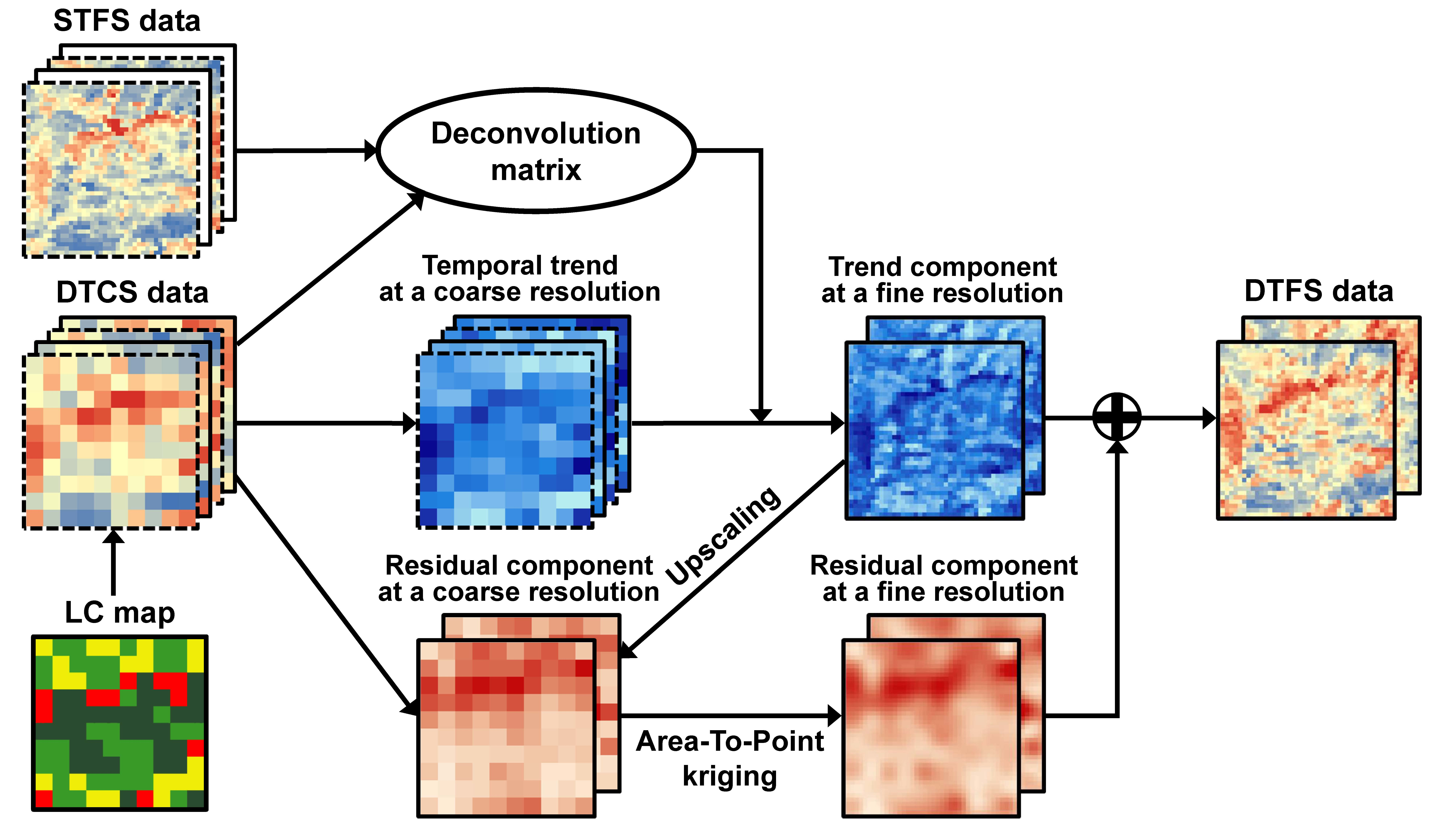
2.1. Generic Formulation

Suppose $\left\{z^C\left(v_i,t_d\right), i=1,\cdots ,N\right\}$ and $\{z^F\left(u_j,t_s\right), j=1,\cdots , M\}$ are target random variables of the DTCS and STFS datasets, respectively, where $v_i$ and $u_j$ denote the $i$th and $j$th coarse resolution and fine resolution pixels, respectively. They are modeled as a joint realization of a collection of spatially correlated time-series within a spatial time-series framework [29]. Note that the acquisition dates of DTCS and STFS data (i.e., $t_d$ and $t_s$, respectively) are usually different, and there is a at least one pair date ($t_s\subseteq t_d)$.

STGDFM aims to generate synthetized DTFS data ($z^F\left(u_j,t_d\right))$ on the prediction date by fully utilizing the information from the DTCS and STFS datasets. Theoretically, the target random variables at certain spatial and temporal resolutions are decomposed into a deterministic trend component and a stochastic residual component,

$$z^C\left(v_i,t_d\right)=m^C\left(v_i,t_d\right)+r^C\left(v_i,t_d\right),$$

(1)

$$z^F\left(u_j,t_s\right)=m^F\left(u_j,t_s\right)+r^F\left(u_j,t_s\right),$$

(2)

where $m$ is the trend component, and $r$ is the residual component.

Based on the above decomposition, each component is estimated using information from the DTCS and STFS datasets. Furthermore, specific estimation methods are developed to tackle the practical issues of spatiotemporal fusion (described in the Introduction). Because the entire time-series dataset is available only at a coarse spatial resolution, the temporal trend component at a coarse spatial resolution ($m^C\left(v_i,t_d\right)$ in Equation (1)) is first quantified using the LC map of the study area. The temporal trend component at a fine spatial resolution ($m^F\left(u_j,t_s\right)$ in Equation (2)) is then estimated using the coarse resolution temporal trend component and a resolution matrix constructed from the DTCS and STFS datasets acquired on the pair dates. Furthermore, the residual component ($r^F\left(u_j,t_s\right)$ in Equation (2)) is estimated via area-to-point kriging (ATPK), which is appropriate for COSP. The DTFS data ($z^F\left(u_j,t_s\right)$) are finally obtained by summing the trend and residual components. Figure 1 presents a flowchart for the implementation of the STGDFM, and the detailed descriptions are given in the following subsections.

2.2. Quantification of Temporal Trends at Coarse Spatial Resolution

In this step, a temporal trend component at a coarse spatial resolution, which characterizes long-term temporal variation patterns, is estimated from the entire DTCS dataset by extending the spatial time-series framework [29] to LC-specific time-series modeling. The spatial time-series framework is employed in this study owing to the simplicity and flexibility of its application to cases with or without periodicity and seasonality. It is important to note that if different trend estimation models are applied, then the residual component in Equation (1) will also be different.

Within the spatial time-series framework, elementary temporal profiles in the study area are first established, and the similarity between the temporal profiles and the time-series at each pixel is then quantified [29]. The spatially averaged time-series values over the study area can be used as the elementary temporal profile. However, as spectral responses for a certain time depend heavily on LC types, using an average time-series for the entire study area fails to properly capture LC-dependent changes. To overcome this limitation, the LC-specific spatially averaged time-series are used as elementary temporal profiles in this study. The temporal trend component at a coarse spatial resolution is modeled by quantifying the similarity between the observed time-series value and the LC-specific elementary temporal profile at each coarse spatial resolution.

When there are $S$ LC types in the study area, the spatially averaged time-series value ($\overline{z_s^C}\left(t_d\right)$) of the s-th LC type is first computed by averaging the coarse resolution pixel values corresponding to the same LC type at each DTCS data ($t_d$) acquisition time,

$$\overline{z_s^C}\left(t_d\right)=\frac{1}{N_s}{\displaystyle \sum }_{i=1}^{N_s}{z}^C\left(v_i,t_d\right),s=1,\cdots ,S,$$

(3)

where $N_s$ is the number of coarse resolution pixels assigned to the s-th LC type.

The relationship between the LC-specific elementary temporal profile in Equation (3) and the time-series value at each coarse resolution pixel is then quantified via a regression model,

$$\widehat{z_s^C}\left(v_i,t_d\right)=f\left(\overline{z_s^C}\left(t_d\right)\right),$$

(4)

where $z_s^C\left(v_i,t_d\right)$ is the attribute of DTCS data corresponding to the s-th LC type at a particular acquisition time of $t_d$, and f () denotes a regression function.

A simple linear model may be applied as a regression function in Equation (4) owing to its simplicity. However, it is often difficult to ensure that the temporal variations are linear [25,30], and they are more likely to exhibit non-linear patterns when DTCS data are acquired more frequently. Therefore, in this study, a random forest model [31] is employed as a regression model to account for the non-linear characteristics of the temporal variations.

2.3. Estimation of Temporal Trends at a Fine Spatial Resolution

Once the temporal trends at a coarse spatial resolution have been quantified, the next step is to estimate the trend component at a fine spatial resolution. To tackle this COSP, the difference in the spatial resolution is accounted for using a resolution matrix [32], whereby the local variations in the STFS data acquired at the pair dates can be considered. The use of the resolution matrix equates to relating the desired fine resolution temporal trends to the estimated coarse resolution temporal trends by representing a relationship between DTCS and STFS data acquired on the pair dates.

In this study, two resolution matrices of convolution and deconvolution are used to estimate the fine resolution trend component. The convolution matrix ($C$) refers to a resolution matrix for predicting the attribute of DTCS data from that of STFS data, and the deconvolution matrix ($D$) is an inverse matrix of the convolution matrix. When the attribute values of DTCS and STFS data obtained at a specific pair date ($k$) are presented by $Z_k^C$ and $Z_k^F$, respectively, in a matrix form, the convolution and deconvolution matrices are given as,

$$Z_k^C={\mathrm{CZ}}_k^F+e_k^C,k=1,\cdots ,K,$$

(5)

$$Z_k^F={\mathrm{DZ}}_k^C+e_k^F,k=1,\cdots ,K,$$

(6)

where $e_k^C$ and $e_k^F$ denote noise vectors with sizes of $N$ and $M$, respectively, and the dimensions of $C$ and $D$ are $N\times M$ and $M\times N$, respectively.

After defining the convolution and deconvolution matrices, the next step is to predict the trend component at a fine spatial resolution from the trend component at a coarse spatial resolution, which was quantified in the previous section. Thus, the main focus of this step is to estimate the deconvolution matrix. The convolution matrix is first constructed, and the deconvolution matrix is then estimated as the inverse convolution matrix of the convolution matrix. In this study, the convolution matrix is constructed as a sparse matrix, assuming that a Gaussian kernel-based point spread function (PSF), which is commonly used as the sensor PSF in remote sensing, can be applied for the COSP. The convolution matrix is a non-square matrix; therefore, its inverse matrix cannot be obtained, and a transposed convolution matrix is used instead as the initial deconvolution matrix (${\widehat{D}}_0$) [33]. The optimal deconvolution matrix is then selected as one that minimizes the noise term in Equation (6).

If the DTCS and STFS data are obtained simultaneously on the prediction date ($p$), the deconvolution matrix (${\widehat{D}}_p$) can be calculated from the initial deconvolution matrix by setting the error term ($∆d_p$) to zero,

$${\hat{D}}_k={\hat{D}}_0+∆d_k,$$

(7)

where the error term ($∆d_k$) is estimated to minimize the noise of Equation (6).

However, as there are no true STFS data at the prediction date, it is not feasible to directly estimate the error term and deconvolution matrix. Instead, the iterative optimization procedure for minimizing the error term in Equation (7) is adopted to estimate the deconvolution matrix. The error at the pair dates ($K$) is defined as the difference between deconvoluted DTCS and true STFS on the pair dates as in Equation (8),

$$∆d_k={\hat{D}}_0{Z}_{i,k}^C-Z_{j,k}^F,k=1,\cdots ,K.$$

(8)

The error term at the prediction date is then estimated by calculating a weight ($w_k$) that considers the difference between the prediction date ($p$) and the pair date ($k$) via Equations (9)–(11),

$$w_k=\frac{1/∆t_k}{{{\displaystyle \sum }}_{k=1}^{K}1/∆t_k},$$

(9)

$$∆t_k=\left|t_k-t_p\right|,$$

(10)

$$∆d_k=w_1∆d_1+w_2∆d_2+\cdots +w_k∆d_k.$$

(11)

More specifically, an initial deconvolution matrix for each pair date is first set up using the DTCD and STFS datasets on the corresponding date. The error term in Equation (8) is then calculated for each pair date. Under the assumption that the error at the prediction date is similar to that at the pair date that is close to the prediction date, the temporal distance is computed using Equation (10) and then used as a weighting value in Equation (9). That is, if the specific pair date is close to the prediction date, a higher weighting is assigned to the error term at the specific pair date. Finally, the errors at the prediction date are estimated by a weighted combination of the errors from all the pair dates.

After the errors at the prediction date have been estimated, the optimized deconvolution matrix can be obtained using Equation (7). This optimization of the deconvolution matrix is repeated until the mean squared errors on the prediction date are less than a predefined threshold value. After the iterative process is completed, the deconvolution matrix is applied to temporal information of DTCS data estimated in the first step and the fine resolution trend component on the prediction date ($m^F\left(u_j,t_p\right)$) is finally obtained.

2.4. Estimation of Residuals at a Fine Spatial Resolution

The next analytical step is to estimate the residual component at a fine spatial resolution to fully account for variations in the target attribute at a fine spatial resolution. The consideration of the residual component for spatiotemporal fusion can account for the change information that is not contained in the trend component. As the trend component at a coarse spatial resolution has already been estimated in the first step, the residual component at a coarse spatial resolution is readily available from the DTFS data for the prediction date in Equation (1). Spatial downscaling can then be applied to predict the residual component at a fine spatial resolution. However, the final prediction result, which is the sum of the fine resolution trend and residual components, may not satisfy the consistency or mass-preserving property [34,35]; therefore, the upscaled prediction result may be different from the DTFS data on the prediction date.

Unlike previous studies [28,36], this study employs two specific approaches to satisfy the consistency property. The trend component at a fine spatial resolution is first aggregated to the spatial resolution of the DTFS data by applying the Gaussian PSF. The residual component at a coarse spatial resolution is then computed by subtracting the upscaled trend component from the DTCS data. The residual component at a fine spatial resolution on the prediction date is finally estimated using ATPK, which is a novel kriging algorithm used for spatial downscaling [34]. The ATPK predicts the fine resolution residual component using a linear combination of neighboring coarse resolution residual values,

$$r^F\left(u_j,t_p\right)={{\displaystyle \sum }}_{l=1}^L{\lambda }_l\left(u_j\right)r^C\left(v_l,t_p\right),$$

(12)

where ${\lambda }_l\left(u_j\right)$ is an ordinary kriging weight assigned to neighboring coarse resolution residuals ($r^C\left(v_l,t_p\right)$), and L is the number of neighboring coarse resolution residuals within a predefined search window.

Finally, the prediction result on the prediction date can be obtained by adding the fine resolution residual component ($r^F\left(u_i,t_p\right)$) to the fine resolution trend component ($m^F\left(u_i,t_p\right)$). As the ATPK perfectly satisfies the consistency property, the final prediction result also preserves the consistency property on the prediction date. Therefore, the upscaling of the fine spatial resolution prediction result to the coarse spatial resolution enables a perfect reproduction of DTFS data values.

3. Experimental Design

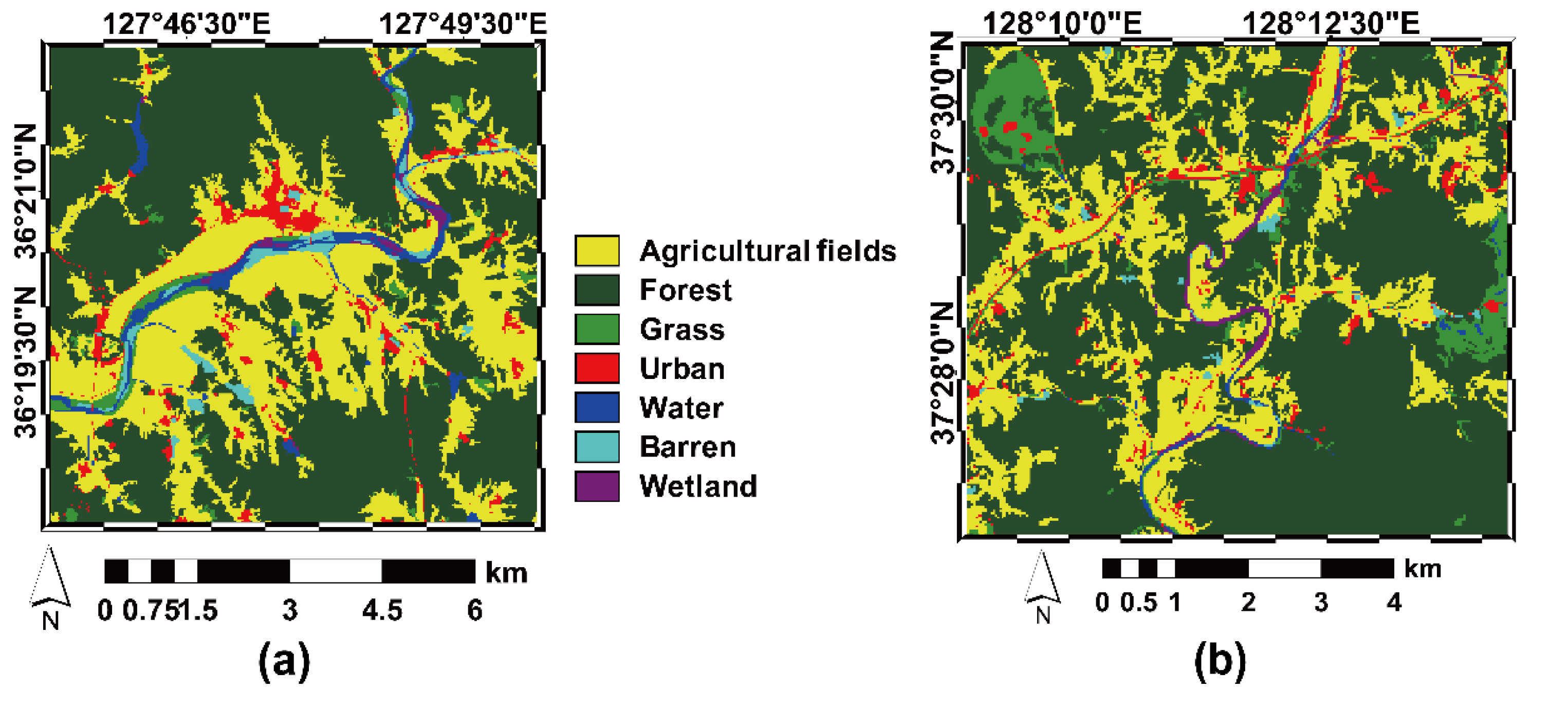
3.1. Study Area and Dataset

The prediction performance of the STGDFM was evaluated via experiments conducted using both spatially degraded datasets and real satellite images. To evaluate how well the STGDFM captures temporal information in DTCS data, the reflectance from an Near InfraRed (NIR) channel (in which temporal variations are more pronounced than in other optical sensor channels) was selected as the target attribute, as in previous studies [18,25,36]. Four study areas within South Korea with different spatial and temporal characteristics were selected for the evaluation study. To conduct the quantitative and objective evaluation and comparison in this study, experiments used both spatially degraded datasets and real satellite images.

3.1.1. Experiments Using Spatially Degraded Datasets

For the experiments using spatially degraded reflectance datasets, we selected two study areas with different temporal variation patterns: a vegetation area (Case 1) and an urban area (Case 2), as illustrated in Figure 2. There were relatively significant temporal variations in the vegetation area, whereas these were comparatively small in the urban area. The LC map from the Ministry of Environment [37] was also used to quantify LC-specific temporal trends.

Daily MODIS data with a high temporal resolution were selected as the main data source. We collected 250 m NIR reflectance data from the MOD09GQ product acquired from February to October in 2018. After excluding cloud-contaminated data, 36 and 40 NIR reflectance datasets were considered as STFS datasets for Cases 1 and 2, respectively (

Table 1. Acquisition dates of dense time-series with coarse spatial resolution (DTCS) data for Case 1; filled circles and open circles denote the pair dates of DTCS and sparse time-series with fine spatial resolution (STFS) data and the prediction dates, respectively.

01 February	04 February	05 February	06 February	07 February	08 February	13 February	15 February	17 February
●		○				○		●
3 March	12 March	14 March	23 March	25 March	26 March	27 March	28 March	10 April
○	○		○				○	○
12 April	18 April	19 April	21 April	28 April	14 May	24 May	26 May	01 June
				○	○	●	○
07 June	22 June	01 August	02 August	12 October	20 October	21 October	30 October	31 October
	○		○	○		○		○

and

Table 2. Acquisition dates of DTCS data for Case 2; Filled circles and open circles denote the pair dates of DTCS and STFS data and the prediction dates, respectively.

15 February	17 February	21 February	26 February	03 March	23 March	25 March	12 April	17 April	18 April
○	●		○	○	○
20 April	21 April	25 April	28 April	04 May	19 May	21 May	23 May	26 May	28 May
				○	○			○
01 June	02 June	16 June	22 June	22 July	17 August	01 September	08 September	24 September	25 September
	○	○		○		○	○	○
29 September	03 October	12 October	13 October	14 October	19 October	20 October	21 October	30 October	31 October
●	○				○				●

). The original 250 m NIR reflectance datasets were upscaled to 1 km using the Gaussian PSF, and the 1 km datasets were then considered as the DTCS datasets. As the true STFS datasets are readily available, it is possible to quantitatively assess and compare the predictive performance of STGDFM with those of other spatiotemporal fusion models.

To mimic a real case with spatially rich but temporally poor datasets, only three dates were selected as the pair dates of the DTCS and STFS datasets for both cases; thus, we assumed that the STFS data were only available on three dates during the considered period. To investigate the impacts of the difference between the pair dates and the prediction date on the predictive performance, 15 dates with different variation patterns over time were selected as the prediction dates (Table 1 and Table 2). The three pairs of datasets and the DTCS data on two prediction dates are presented in Figure 3 and Figure 4.

3.1.2. Experiments Using Real Satellite Images

To further evaluate the STGDFM, experiments were conducted using multiple satellite datasets with different spatial and temporal resolutions. Two areas with different heterogeneous landscape types were selected as the study areas (Cases 3 and 4). As with the experiments conducted on spatially degraded data, the LC map was also used to quantify LC-specific temporal trends (Figure 5).

MODIS and Landsat-7 Enhanced Thematic Mapper Plus (ETM+) images, which have been widely used in previous spatiotemporal fusion studies [13,14,15,16,17,18,19,20,25,26], were employed as the DTCS and STFS data, respectively. Twenty-eight and 32 cloud-free NIR reflectance datasets from February to November 2018 were collected for the areas in Cases 3 and 4, respectively (

Table 3. Acquisition dates of DTCS data for Case 3; Filled circles and open circles denote the pair dates of DTCS and STFS data and the prediction dates, respectively.

01 February	07 February	15 February	03 March	12 March	14 March	25 March
27 March	28 March	08 April	10 April	19 April	10 May	24 May
					●
26 May	01 June	02 June	06 June	16 June	22 June	03 October
●
12 October	13 October	17 October	19 October	21 October	24 October	30 October
		○

and

Table 4. Acquisition dates of DTCS data for Case 4; Filled circles and open circles denote the pair dates of DTCS and STFS data and the prediction dates, respectively.

01 February	05 February	07 February	17 February	12 March	23 March	25 March	28 March
					○
10 April	19 April	21 April	28 April	29 April	21 May	24 May	26 May
							●
02 June	06 June	16 June	22 June	22 July	02 August	08 September	03 October
12 October	21 October	24 October	31 October	02 November	04 November	20 November	30 November
				●

). Landsat images were downloaded from the U.S. Geological Survey Earth Resources Observation and Science Center [38]. By considering the spatial resolution of Landsat data (30 m), the original 250 m MODIS data were resampled to 240 m using a nearest neighbor method.

Unlike in the experiments conducted on spatially degraded datasets, the prediction performance of spatiotemporal fusion models can only be quantitatively assessed when Landsat data are acquired. There were only three pairs of datasets for both Cases 3 and 4. For Case 3, the prediction date was selected as 17 October, when the spatial patterns of different LC types were significantly different from those of the other two dates, as presented in Figure 6.

The prediction date of Case 4 was selected as 23 March; the difference between the pair dates and the prediction date was thus large, and the spatial pattern also differed significantly from the closest pair date (Figure 7).

3.2. Evaluation Method

The performance of STGDFM was evaluated through comparisons with those of STARFM and ESTAFM, which have been widely applied in comparative studies. With visual inspections of true STFS data and prediction results, we computed two quantitative indices for quantitative comparisons: (1) root mean squared error (RMSE) and (2) structure similarity (SSIM). The RMSE was computed to compare the magnitude of prediction errors and the SSIM was used to compare the spatial similarity between true STFS data and the prediction results. SSIM is a quantitative index to measure the spatial similarity between two images [39], and it ranges from 0 to 1—the closer it is to 1, the greater is the spatial similarity between the two images.

4. Results

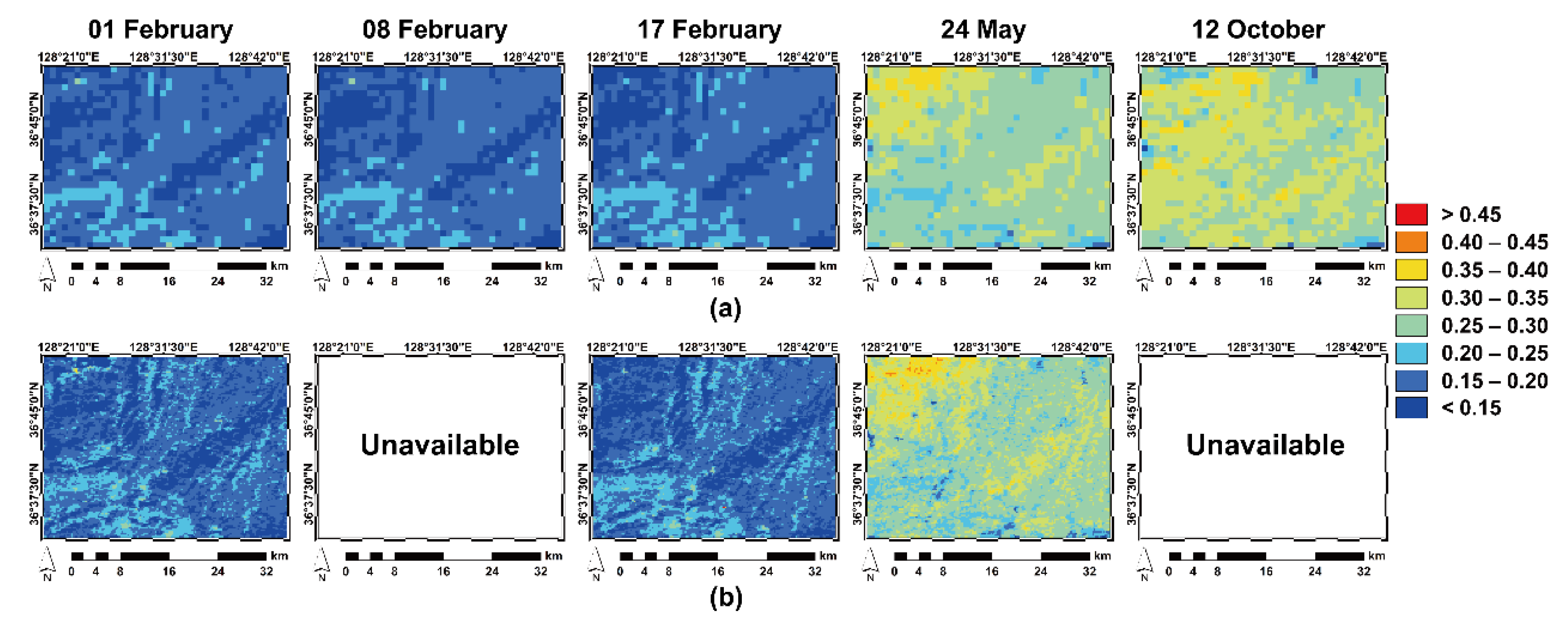
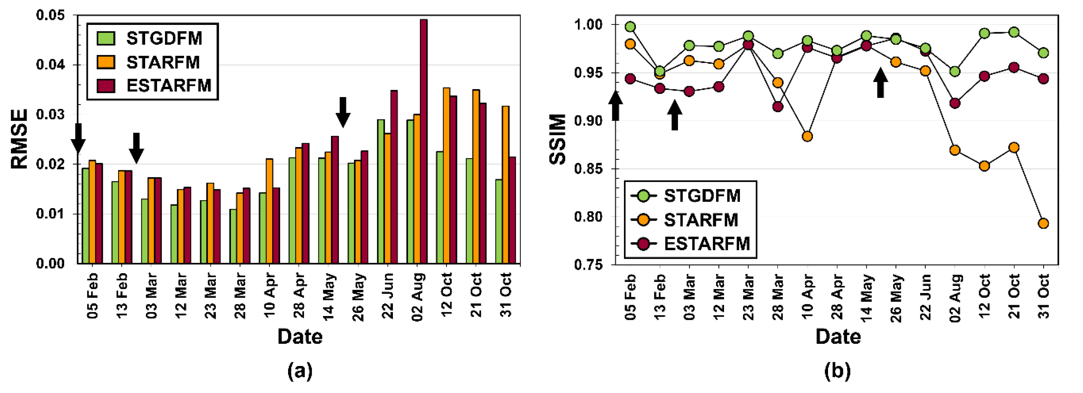
4.1. Results for Experiments Conducted on Spatially Degraded Datasets

Figure 8 presents the RMSEs and SSIMs for the prediction results from the three spatiotemporal fusion models for Case 1, where it is evident that there were no significant differences in the prediction performances between the three spatiotemporal fusion models when the pair dates and the prediction date were close. However, with a larger difference between the pair dates and the prediction date, the prediction performance of STGDFM was superior to those of STARFM and ESTARFM, particularly in October. For example, on 12 October, STGDFM and STARFM provided the best and worst model performance, respectively, and STGDFM yielded significant RMSE and SSIM improvements in comparison with STARFM (RMSE and SSIM improvements of 34.3% and 13.93%, respectively). The inferior prediction performance of STARFM and ESTARFM are a result of the smoothing out of local details, as illustrated in Figure 9. Low values and large values were over- and under-estimated in the results from STARFM and ESTARFM, respectively, particularly in the upper left corner of the study area. However, local spatial variation details of the attribute were well reproduced in STGDFM, and a lower RMSE and higher SSIM were achieved.

As in Case 1, there were significant differences in the prediction performances between three models in Case 2 when the difference between the pair dates and the prediction date increased (Figure 10). The prediction performance of STARFM was the worst and that of STGDFM was slightly better than that of ESTARFM. The RMSE values of ESTARFM were slightly smaller than those of STGDFM for some prediction dates, but STGDFM provided the largest SSIM on those dates. For example, STGDFM provided a slightly larger RMSE than ESTARFM on 19 May (0.035 vs. 0.032, respectively). A visual assessment of the prediction results using true STFS data (Figure 11) indicated that the spatial patterns of ESTARFM were significantly different from those of the true STFS data, and most of the large values in the forests seen in Figure 11a were smoothed out and underestimated in ESTARFM (Figure 11d).

In contrast, STGDFM reproduced most of the spatial features with large and small values, as presented in Figure 11b; furthermore, the SSIM value of STGDFM was larger than that of ESTARFM (0.981 vs. 0.950, respectively). However, some of the over-estimated spatial patterns in the STGDFM result caused a slightly larger RMSE value compared to that of ESTARFM, but the difference was not very significant.

The results of Cases 1 and 2 indicate that STARFM and ESTARFM tend to smooth out local details of spatial features, whereas STGDFM can alleviate the smoothing effects and reproduce spatial patterns that have large and small values. This advantage of STGDFM over STARFM and ESTARFM is more prominent when the difference between the pair dates and the prediction date increases.

4.2. Results for the Experiment on Real Satellite Images

For Case 3, where spatial patterns on the prediction date differ much from those of the pair datasets, we first visually compared true STFS data acquired on 17 October with the prediction results of the three models (Figure 12). Overall, STGDFM yielded spatial patterns similar to those of true STFS data, whereas STARFM and ESTARFM presented locally smoothed and clustered variations, and there were particular under-estimations in the southern part of the study area. As STARFM and ESTARFM use information only from the pair datasets and the DTCS data acquired on the prediction date, the dominant impacts of DTCS data on the prediction date resulted in the under-estimated predictions by STARFM and ESTARFM (see Figure 6 and Figure 12). Particularly, the spectral discrepancy between the pair dates and the prediction date was greatest for areas of forest. The smaller DTCS data values for the prediction date were highly reflected into the prediction results by STARFM and ESTARFM. In contrast, the STGDFM reduced the strong impact of DTCS data on the prediction date by fully accounting for the continuous temporal evolution information obtained from the entire DTCS dataset.

The quantitative assessment results of the three models presented in

Table 5. Quantitative evaluation statistics of three spatiotemporal fusion models.

		STGDFM	STARFM	ESTARFM
Case 3	RMSE	0.0511	0.0579	0.0554
	SSIM	0.935	0.924	0.943
Case 4	RMSE	0.0264	0.0492	0.0315
	SSIM	0.961	0.845	0.856

indicate that STARFM provided the worst performance in Case 3, and STGDFM delivered the best prediction accuracy with RMSE improvements of 11.74% and 7.76% over STARFM and ESTARFM, respectively. However, ESTARFM provided the largest SSIM, indicating that it well represented the spatial structure of the true STFS data. The SSIM value of STGDFM was lower than that of ESTARFM, even though it provided the best RMSE value, and this result contradicts the visual assessment results. A detailed analysis of this contradictory result was then conducted to compare the SSIM values of STGDFM and ESTARFM within two major LC types (cropland and forest) in the study area. The SSIM values within the cropland and forest between STGDFM and ESTARFM were 0.952 vs. 0.900, and 0.828 vs. 0.938, respectively. The SSIM of STGDFM was greater than that of ESTARFM within the cropland, whereas ESTARM delivered a greater SSIM than STGDFM within the forest, yielding the largest SSIM of ESTARFM throughout the study area. The lower SSIM value of STGDFM was particularly attributed to under-estimation of larger values in the northeastern part of the study area (see Figure 12). The forest class in the study area consists of various forest types, including deciduous, coniferous, and mixed forests. ESTARFM considered the different LC types via unmixing. However, STGDFM considered only one forest class when estimating the temporal trend component, and the different temporal spectral variations of the three different forest types could not be properly estimated, which yielded a lower SSIM value for STGDFM. Nevertheless, this lower SSIM can be improved using LC maps containing various LC types. This issue will be further described in the Discussion section.

Figure 13 presents the prediction results for Case 4, where the spatial patterns on the prediction date were similar to those of the pair datasets. As in Case 3, the prediction results of STGDFM represented its ability to reproduce the spatial pattern of the true STFS data, whereas those of STARFM and ESTARFM yielded prediction results in which the spatial patterns of STFS data on 2 November were more prominent (compare Figure 7 and Figure 13). As STARFM and ESTARFM are theoretically based on the weighted combination of pair datasets, high weights are assigned to data that have relatively similar spectral characteristics. Therefore, the spatial patterns of STFS data acquired on 2 November were strongly reflected in the prediction results. In contrast, STGDFM alleviated this dominant effect of data on 2 November through residual correction. The residual component that could not be explained by temporal evolution information included temporary information relating to changes on the prediction date, which yielded prediction results that were similar to those of true STFS data. As with the visual assessment results, STGDFM delivered the best prediction performance and provided both relatively lower RMSE and higher SSIM values, in comparison with STARFM and ESTARFM (see Table 5).

From the results of Cases 3 and 4 with real datasets, the prediction results of STARFM and ESTARFM were found to be strongly affected by the pair datasets and the DTCS data on the prediction date. When there is a large difference between the spatial patterns of the pair datasets and the DTCS data on the prediction date (Case 3), the spatial patterns in the DTCS data on the prediction date significantly affect the prediction result. When spatial patterns in the pair datasets and the DTCS data on the prediction are similar, as in Case 4, the spatial pattern in the pair datasets has a considerable impact on the prediction results. Consequently, it may be difficult to capture spatial variations that are not observed in the pair datasets but have to be predicted. In contrast, STGDFM can account for both the residual component and temporal evolution information from the entire DTCS dataset; thus, it can deliver the best prediction performance.

5. Discussion

5.1. Novelty of STGDFM

The prediction performance of STGDFM was thoroughly evaluated by conducting extensive experiments using distinctive cases as follows: (1) cases in which the spectral variations between the pair dates and the prediction date are large (Cases 1 and 3); (2) cases in which the spectral variations between the pair dates and the prediction date are not large (Cases 2 and 4). As a result, the best prediction performance was delivered by STGDFM. The superiority of STGDFM can be attributed to two distinctive procedures included within it. First, STGDFM properly considers the LC-specific temporal information conveyed by the entire DTCS datasets when estimating the trend component. STARFM and ESTARFM quantify the temporal information by using only the pair datasets [13,14], whereas STGDFM models quantitative information relating to continuous temporal variations using the entire DTCS datasets. Specifically, the temporal profiles of reflectance are quantified with respect to different LC types and considered as temporal evolution information. The temporal trend components at a fine spatial resolution are then estimated using temporal evolution information from the DTCS datasets and the STFS data on pair dates. These procedures enable temporal spectral variations at fine resolution pixels to be employed, which then provide a superior prediction performance. In particular, when the spectral variations between the pair dates and the prediction date are large, the temporal trend component contributes to improving the prediction performance (Figure 9 and Figure 12). In contrast, the experiments using spatially degraded datasets revealed that pair datasets have to be collected at times close to the prediction date for STARFM and ESTARFM (Figure 8 and Figure 10). From a practical perspective, however, it is not always possible to collect optical images at specified times of interest due to atmospheric conditions. Therefore, STGDFM, with its distinctive properties, such as the ability to consider the temporal trend components quantified from entire DTCS datasets, provides major advantages over conventional spatiotemporal fusion models.

In some cases, temporary variations that cannot be captured by the temporal trend components may be observed in the datasets [36]. In particular, when there are not considerable differences between the spectral patterns on pair dates and prediction dates (Cases 2 and 4), there may not be significant differences in the temporal trend components, as these are already quantified as spatially averaged temporal profiles. Consequently, the impact of temporary variations may be greater on the prediction result; this implies that the temporary variations should be properly considered to generate reliable prediction results. The local variability of temporal change is considered as the residual component in STGDFM. It is thus necessary to consider the residual components or residual correction, together with the temporal trend component estimation. The necessity of residual correction can be further illustrated using the results from Case 4. In Case 4, the spectral patterns on the pair dates and the prediction dates are similar, and the fine resolution trend component estimated by STGDFM on 23 March for Case 4 (Figure 14) shows low reflectance in forest areas due to the impact of the STFS data on 2 November (Figure 7b). However, STGDFM generates the prediction result by adding the fine resolution residual component to the fine resolution temporal trend component, which is similar to the true DTFS data (Figure 13a,b). Because STARFM and ESTARFM assign higher weights to the pair dataset for Case 4 [13,14,36], the spatial patterns in the prediction results are similar to those in the pair data, but these are much different from those of the true DTFS data (see Figure 13).

In summary, the spectral changes occurring between pair dates and prediction dates can be divided into temporal spectral patterns and temporary variations. In STGDFM, the temporal spectral patterns are quantified by the LC-specific temporal trend component, and the temporary variations or abrupt changes that cannot be reflected in the trend component are accounted for by residual correction. These novel schemes enable its improved prediction performance in comparison with STARFM and ESTARFM in the experiments conducted here.

5.2. Further Improvement of STGDFM

Despite the superior prediction performance of STGDFM, certain aspects require further modification and improvement. For example, the effect of only one coarse resolution pixel including several fine resolution pixels within it is assumed to exist when estimating the fine resolution trend component, which could generate blocky artifacts in the fine resolution trend component estimation result. Consequently, the final DTFS result may include blocky artifacts, depending on the contribution from residual correction. In addition to the one coarse resolution pixel, neighboring coarse resolution pixels may affect the estimation of fine resolution attributes from coarse resolution pixels [40]. To alleviate the impacts of blocky artifacts from the coarse resolution pixels, a weighted combination of neighboring coarse resolution pixels should be considered.

Two critical issues in spatiotemporal fusion are how to effectively model (1) landscape heterogeneity and (2) abrupt LC changes [41]. Regarding the issue on landscape heterogeneity, STGDFM generated locally different prediction results primarily observed in areas with different forest types, as described in the result for Case 3. Some LC types consist of several sub-classes, for example, agricultural land with paddy rice fields and dry fields, but only typical LC types (forest and agricultural land) were considered in STGDFM. However, the temporal trend components of several LC types can be easily estimated within the STGDFM framework without modifying the modeling procedures, provided that LC maps with detailed sub-classes are available and that there are sufficient numbers of pixels for the sub-classes within the study area. To evaluate the impact of using LC maps with detailed sub-classes on prediction performance of STGDFM, fine resolution level-2 LC maps with several sub-classes in forest and agricultural land (Figure 15) [37] were used for Case 3. STGDFM with the detailed LC map showed superior predictions relative to that with the LC map in Figure 5a (RMSE: 0.0501 vs. 0.0511 and SSIM: 0.945 vs. 0.935). Moreover, the SSIM value of STGDFM with the detailed LC map was slightly better than or compatible to that of ESTARFM (0.943). Therefore, when temporal trends of sub-LC types are different like Case 3, using the detailed LC map could improve the prediction performance of STGDFM.

Even when various LC types are considered in STGDFM, temporal trends are estimated from DTCS data in STGDFM. Hence, mixed pixel problems, which are frequently encountered in coarse resolution remote sensing images and prominent in heterogeneous regions, may affect the temporal trends estimated at a coarse spatial resolution. Conventional spatiotemporal fusion models, such as ESTARFM, explicitly address the mixed pixel effect via spectral unmixing [14]. Because STDGFM does not explicitly account for the mixed pixel effect, specific analytical procedures should be incorporated into STDGFM to address heterogeneous pixel problems. Class fraction or composition of a coarse resolution pixel can be first computed using spectral unmixing or existing land-cover maps [42,43]. This sub-pixel fraction information can then be used as a constraint to estimate the optimized deconvolution matrix.

The second critical issue in spatiotemporal fusion is how well any fusion model captures abrupt LC changes, such as floods and wildfires [27,36]. STGDFM could capture well gradual spectral changes, such as vegetation phenology, because temporal evolution information is modeled from the entire DTCS datasets. If abrupt LC changes occurred in the study area, they are likely to alter LC-specific elementary temporal profile in STGDFM. However, the temporal trend component at a coarse spatial resolution estimated by regression with respect to the LC-specific elementary temporal profile may not contain the LC change information fully. STGDFM assumes that such the change information that cannot be captured in the trend component is contained in the residual component, similar to previous studies [27,28,36]. Although residual correction helps capture abrupt LC changes to a certain extent, further improvement of STGDFM is required to fully account for LC change information. Recently, Zhou and Zhong [41] proposed a Kalman filter reflectance fusion model (KFRFM) that can fully account for both abrupt LC changes and landscape heterogeneity. KFRFM could properly capture abrupt LC changes by progressively generating a DTFS dataset using reflectance change rates between consecutive DTCS data. Similar to KFRFM, STGDFM can generate such a continuous DTFS dataset on the DTCS data acquisition dates. Abrupt LC changes can thus be captured in STGDFM by both the continuous DTFS dataset and residual correction. The improvement of STGDFM by considering both landscape heterogeneity and abrupt LC changes and comparisons with the recent state-of-the-art spatiotemporal fusion models, including KFRFM, will be included in future work.

In this study, STGDFM was applied to the NIR band to quantify how well it can account for the temporal evolution of spectral variations mainly in forest and agricultural areas, like previous spatiotemporal fusion studies [44,45]. STGDFM can be applied to other spectral bands, such as red and green bands, and satellite-derived products containing significant temporal changes (vegetation index, land surface temperature, and soil moisture) without modifying the modeling procedures of STGDFM. The application to such different data is worth evaluating through extensive experiments to increase the applicability and validity of STGDFM.

6. Conclusions

Spatiotemporal fusion in remote sensing aims to generate synthesized data at high temporal and spatial resolutions by capturing both dense temporal features from the DTCS data and local details from the STFS data. This study presented a spatial time-series geostatistical fusion model with three analytical procedures, named STGDFM. The LC-specific temporal profiles of reflectance are considered to model temporal evolution information of spectral variations from the entire DTCS dataset. During this temporal trend estimation procedure, local variations in the STFS data are properly considered using the resolution matrix. Furthermore, residual correction via ATPK is considered to both reflect fine scale spectral variability on the prediction date and to preserve the consistency property.

Comparative experiments were conducted using conventional spatiotemporal fusion models, STARFM and ESTARFM, and STGDFM was found to deliver prediction result that were similar to those of the true data. It thus provided the best consistent predictive performance, irrespective of the similarity between spatial patterns of pair datasets and DTCS data on the prediction date. In addition, the superiority of STGDFM compared to STARFM and ESTARFM was found to be particularly prominent when there was an increased difference between the pair dates and the prediction dates, and this confirmed the potential of STGDFM for consistent environmental monitoring. To strengthen the applicability of STGDFM, future work will consider (1) the application to satellite-derived products and other spectral bands and (2) the refinement of modeling procedures to explicitly address both landscape heterogeneity and abrupt LC changes.

References

1. Ghamisi, P.; Rasti, B.; Yokoya, N.; Wang, Q.; Höfle, B.; Bruzzone, L.; Bovolo, F.; Chi, M.; Anders, K.; Gloaguen, R.; et al. Multisource and multitemporal data fusion in remote sensing: A comprehensive review of the state of the art. IEEE Geosci. Remote Sens. Mag. 2019, 7, 6–39. [Google Scholar] [CrossRef] [Green Version]
2. Park, N.-W.; Kim, Y.; Kwak, G.-H. An overview of theoretical and practical issues in spatial downscaling of coarse resolution satellite-derived products. Korean J. Remote Sens. 2019, 35, 589–607. [Google Scholar]
3. Kim, Y.; Park, N.-W.; Lee, K.-D. Self-learning based land-cover classification using sequential class patterns from past land-cover maps. Remote Sens. 2017, 9, 921. [Google Scholar] [CrossRef] [Green Version]
4. Park, N.-W.; Kyriakidis, P.C.; Hong, S. Geostatistical integration of coarse resolution satellite precipitation products and rain gauge data to map precipitation at fine spatial resolutions. Remote Sens. 2017, 9, 255. [Google Scholar] [CrossRef] [Green Version]
5. Zheng, Q.; Wang, Y.; Chen, L.; Wang, Z.; Zhu, H.; Li, B. Inter-comparison and evaluation of remote sensing precipitation products over China from 2005 to 2013. Remote Sens. 2018, 10, 168. [Google Scholar] [CrossRef] [Green Version]
6. Arulraj, M.; Barros, A.P. Improving quantitative precipitation estimates in mountainous regions by modelling low-level seeder-feeder interactions constrained by global precipitation measurement dual-frequency precipitation radar measurements. Remote Sens. Environ. 2019, 231, 111213. [Google Scholar] [CrossRef]
7. Jung, M.; Lee, S.-H. Application of multi-periodic harmonic model for classification of multi-temporal satellite data: MODIS and GOCI imagery. Korean J. Remote Sens. 2019, 35, 573–587. [Google Scholar]
8. Deng, C.; Zhu, Z. Continuous subpixel monitoring of urban impervious surface using Landsat time series. Remote Sens. Environ. 2018, 238, 110929. [Google Scholar] [CrossRef]
9. Cahalane, C.; Magee, A.; Monteys, X.; Casal, G.; Hanafin, J.; Harris, P. A comparison of Landsat 8, RapidEye and Pleiades products for improving empirical predictions of satellite-derived bathymetry. Remote Sens. Environ. 2019, 233, 111414. [Google Scholar] [CrossRef]
10. Sun, W.; Fan, J.; Wang, G.; Ishidaira, H.; Bastola, S.; Yu, J.; Fu, Y.H.; Kiem, A.S.; Zuo, D.; Xu, Z. Calibrating a hydrological model in a regional river of the Qinghai-Tibet plateau using river water width determined from high spatial resolution satellite images. Remote Sens. Environ. 2018, 214, 100–114. [Google Scholar] [CrossRef]
11. Filipponi, F. Exploitation of Sentinel-2 time series to map burned areas at the national level: A case study on the 2017 Italy wildfires. Remote Sens. 2019, 11, 622. [Google Scholar] [CrossRef] [Green Version]
12. Furberg, D.; Ban, Y.; Nasacetti, A. Monitoring of urbanization and analysis of environmental impact in Stockholm with Sentinel-2A and SPOT-5 multispectral data. Remote Sens. 2019, 11, 2408. [Google Scholar] [CrossRef] [Green Version]
13. Gao, F.; Masek, J.; Schwaller, M.; Hall, F. On the blending of the Landsat and MODIS surface reflectance: Predicting daily Landsat surface reflectance. IEEE Trans. Geosci. Remote Sens. 2006, 44, 2207–2218. [Google Scholar]
14. Zhu, X.; Chen, J.; Gao, F.; Chen, X.; Masek, J.G. An enhanced spatial and temporal adaptive reflectance fusion model for complex heterogeneous regions. Remote Sens. Environ. 2010, 114, 2610–2623. [Google Scholar] [CrossRef]
15. Ibnelhobyb, A.; Mouak, A.; Radgui, A.; Tamtaoui, A.; Er-Raji, A.; Hadani, D.E.; Merdas, M.; Smiej, F.M. New wavelet based spatiotemporal fusion method. In Proceedings of the Fifth International Conference on Telecommunications and Remote Sensing (ICTRS 2016), Milan, Italy, 10–11 October 2016; pp. 25–32. [Google Scholar]
16. Emelyanova, I.V.; McVicar, T.R.; Van Niel, T.G.; Li, L.T.; Van Dijk, A.I.J.M. Assessing the accuracy of blending Landsat-MODIS surface reflectances in two landscapes with contrasting spatial and temporal dynamics: A framework for algorithm selection. Remote Sens. Environ. 2013, 133, 193–209. [Google Scholar] [CrossRef]
17. Ma, J.; Zhang, W.; Marinoni, A.; Gao, L.; Zhang, B. An improved spatial and temporal reflectance unmixing model to synthesize time series of Landsat-like images. Remote Sens. 2018, 10, 1388. [Google Scholar] [CrossRef] [Green Version]
18. Gevaert, C.M.; García-Haro, F.J. A comparison of STARFM and an unmixing-based algorithm for Landsat and MODIS data fusion. Remote Sens. Environ. 2015, 156, 34–44. [Google Scholar] [CrossRef]
19. Huang, B.; Song, H. Spatiotemporal reflectance fusion via sparse representation. IEEE Trans. Geosci. Remote Sens. 2012, 50, 3707–3716. [Google Scholar] [CrossRef]
20. Song, H.; Huang, B. Spatiotemporal satellite image fusion through one-pair image learning. IEEE Trans. Geosci. Remote Sens. 2013, 51, 1883–1896. [Google Scholar] [CrossRef]
21. Liu, X.; Deng, C.; Wang, S.; Huang, G.-B.; Zhao, B.; Lauren, P. Fast and accurate spatiotemporal fusion based upon extreme learning machine. IEEE Geosci. Remote Sens. Lett. 2016, 13, 2039–2043. [Google Scholar] [CrossRef]
22. Tan, Z.; Yue, P.; Di, L.; Tang, J. Deriving high spatiotemporal remote sensing images using deep convolutional network. Remote Sens. 2018, 10, 1066. [Google Scholar] [CrossRef] [Green Version]
23. Yang, J.; Wright, J.; Huang, T.S.; Ma, Y. Image super-resolution via sparse representation. IEEE Trans. Image Process. 2010, 19, 2861–2873. [Google Scholar] [CrossRef] [PubMed]
24. Zhao, Y.; Huang, B.; Song, H. A robust adaptive spatial and temporal image fusion model for complex land surface changes. Remote Sens. Environ. 2018, 208, 42–62. [Google Scholar] [CrossRef]
25. Xue, J.; Leung, Y.; Fung, T. A Bayesian data fusion approach to spatio-temporal fusion of remotely sensed images. Remote Sens. 2017, 9, 1310. [Google Scholar] [CrossRef] [Green Version]
26. Xue, J.; Leung, Y.; Fung, T. An unmixing-based Bayesian model for spatio-temporal satellite image fusion in heterogeneous landscapes. Remote Sens. 2019, 11, 324. [Google Scholar] [CrossRef] [Green Version]
27. Zhong, D.; Zhou, F. A prediction smooth method for blending Landsat and Moderate Resolution Imagine Spectroradiometer Images. Remote Sens. 2018, 10, 1371. [Google Scholar] [CrossRef] [Green Version]
28. Zhong, D.; Zhou, F. Improvement of clustering methods for modelling abrupt land surface changes in satellite image fusions. Remote Sens. 2019, 11, 1759. [Google Scholar] [CrossRef] [Green Version]
29. Kyriakidis, P.C.; Miller, N.L.; Kim, J. A spatial time series framework for simulating daily precipitation at regional scales. J. Hydrol. 2004, 297, 236–255. [Google Scholar] [CrossRef]
30. Qin, Y.; Li, B.; Chen, Z.; Chen, Y.; Lian, L. Spatio-temporal variations of nonlinear trends of precipitation over an arid region of northwest China according to the extreme-point symmetric model decomposition method. Int. J. Climatol. 2018, 38, 2239–2249. [Google Scholar] [CrossRef]
31. Breiman, L. Random forests. Mach. Learn. 2001, 45, 5–32. [Google Scholar] [CrossRef] [Green Version]
32. Zhang, H.; Zhang, L.; Shen, H. A super-resolution reconstruction algorithm for hyperspectral images. Signal Process. 2012, 92, 2082–2096. [Google Scholar] [CrossRef]
33. Dumoulin, V.; Visin, F. A guide to convolution arithmetic for deep learning. arXiv 2016, arXiv:1603.07285. [Google Scholar]
34. Kyriakidis, P.C. A geostatistical framework for area-to-point spatial interpolation. Geogr. Anal. 2004, 36, 259–289. [Google Scholar] [CrossRef]
35. Goovaerts, P. Kriging and semivariogram deconvolution in the presence of irregular geographical units. Math. Geosci. 2008, 40, 101–128. [Google Scholar] [CrossRef] [Green Version]
36. Zhu, X.; Helmer, E.H.; Gao, F.; Liu, D.; Chen, J.; Lefsky, M.A. A flexible spatiotemporal method for fusing satellite images with different resolutions. Remote Sens. Environ. 2016, 172, 165–177. [Google Scholar] [CrossRef]
37. EGIS (Environmental Geographic Information Service). Available online: https://egis.me.go.kr (accessed on 1 May 2019).
38. U.S. Geological Survey (USGS) Earth Resources Observation and Science (EROS) Center. Available online: http://earthexplorer.usgs.gov (accessed on 1 May 2019).
39. Wang, Z.; Bovik, A.C.; Sheikh, H.R.; Simoncelli, E.P. Image quality assessment: From error visibility to structural similarity. IEEE Trans. Image Process. 2004, 13, 600–612. [Google Scholar] [CrossRef] [Green Version]
40. Wang, Q.; Atkinson, P.M. The effect of the point spread function on sub-pixel mapping. Remote Sens. Environ. 2017, 193, 127–137. [Google Scholar] [CrossRef] [Green Version]
41. Zhou, F.; Zhong, D. Kalman filter method for generating time-series synthetic Landsat images and their uncertainty from Landsat and MODIS observation. Remote Sens. Environ. 2020, 239, 111628. [Google Scholar] [CrossRef]
42. Zhang, Y.; Foody, G.M.; Ling, F.; Li, X.; Ge, Y.; Du, Y.; Atkinson, P.M. Spatial-temporal fraction map fusion with multi-scale remotely sensed images. Remote Sens. Environ. 2018, 213, 162–181. [Google Scholar] [CrossRef]
43. Li, X.; Foody, G.M.; Boyd, D.S.; Ge, Y.; Zhang, Y.; Du, Y.; Ling, F. SFSDAF: An enhanced FSDAF that incorporates sub-pixel class fraction change information for spatio-temporal image fusion. Remote Sens. Environ. 2020, 237, 111537. [Google Scholar] [CrossRef]
44. Onojeghuo, A.O.; Blackburn, G.A.; Wang, Q.; Atkinson, P.M.; Kindred, D.; Miao, Y. Rice crop phenology mapping at high spatial and temporal resolution using downscaled MODIS time-series. GISci. Remote Sens. 2018, 55, 659–677. [Google Scholar] [CrossRef] [Green Version]
45. Zhou, X.; Wang, P.; Tansey, K.; Zhang, S.; Li, H.; Wang, L. Developing a fused vegetation temperature condition index for drought monitoring at field scales using Sentinel-2 and MODIS imagery. Comput. Electron. Agric. 2020, 168, 105144. [Google Scholar] [CrossRef]
Figure 1. Flowchart of the proposed spatiotemporal fusion model (STGDFM). The data acquired on the prediction date and pair dates are denoted using squares with solid and dashed lines, respectively. DTCS = dense time-series with coarse spatial resolution; STFS = sparse time-series with fine spatial resolution; LC = land-cover; DTFS = dense time-series with fine spatial resolution.
Remotesensing 12 01553 g001
Figure 2. Study areas and land-cover (LC) maps for experiments conducted on spatially degraded datasets: (a) Case 1; and (b) Case 2.
Remotesensing 12 01553 g002
Figure 3. Input datasets for Case 1: (a) upscaled MODIS data acquired on pair and prediction dates; and (b) original MODIS data acquired on the pair dates.
Remotesensing 12 01553 g003
Figure 4. Input datasets for Case 2: (a) upscaled MODIS data acquired on pair and prediction dates; and (b) original MODIS data acquired on the pair dates.
Remotesensing 12 01553 g004
Figure 5. Study areas and LC maps for experiments conducted using real satellite images: (a) Case 3; and (b) Case 4.
Remotesensing 12 01553 g005
Figure 6. Some of the input data used in Case 3: (a) MODIS data on pair and prediction dates; and (b) Landsat data acquired on pair dates.
Remotesensing 12 01553 g006
Figure 7. Some of the input data used in Case 4: (a) MODIS data on pair and prediction dates; and (b) Landsat data on pair dates.
Remotesensing 12 01553 g007
Figure 8. Comparison of root mean squared error (RMSE) and structure similarity (SSIM) values between three different models for all prediction dates of Case 1: (a) RMSE; and (b) SSIM (arrows indicate pair dates).
Remotesensing 12 01553 g008
Figure 9. Spatial patterns of the true data and prediction results on 12 October for Case 1: (a) true data; (b) spatial time-series geostatistical deconvolution/fusion model (STGDFM); (c) spatial and temporal adaptive reflectance fusion model (STARFM); and (d) enhanced STARFM (ESTARFM).
Remotesensing 12 01553 g009
Figure 10. Comparison of RMSE and SSIM values between three different models for all prediction dates of Case 2: (a) RMSE; and (b) SSIM (arrows indicate pair dates).
Remotesensing 12 01553 g010
Figure 11. Spatial patterns of the true data and prediction results on 19 May for Case 2: (a) true data; (b) STGDFM; (c) STARFM; and (d) ESTARFM.
Remotesensing 12 01553 g011
Figure 12. Spatial patterns of the true data and prediction results on 17 October for Case 3: (a) true data; (b) STGDFM; (c) STARFM; and (d) ESTARFM.
Remotesensing 12 01553 g012
Figure 13. Spatial patterns of the true data and prediction results on 23 March for Case 4: (a) true data; (b) STGDFM; (c) STARFM; and (d) ESTARFM.
Remotesensing 12 01553 g013
Figure 14. Fine resolution trend component of STGDFM on 23 March for Case 4.
Remotesensing 12 01553 g014
Figure 15. Fine resolution level-2 LC map for Case 3.
Remotesensing 12 01553 g015