Land Cover Classification of Nine Perennial Crops Using Sentinel-1 and -2 Data

Abstract

Land cover mapping of intensive cropping areas facilitates an enhanced regional response to biosecurity threats and to natural disasters such as drought and flooding. Such maps also provide information for natural resource planning and analysis of the temporal and spatial trends in crop distribution and gross production. In this work, 10 meter resolution land cover maps were generated over a 6200 km² area of the Riverina region in New South Wales (NSW), Australia, with a focus on locating the most important perennial crops in the region. The maps discriminated between 12 classes, including nine perennial crop classes. A satellite image time series (SITS) of freely available Sentinel-1 synthetic aperture radar (SAR) and Sentinel-2 multispectral imagery was used. A segmentation technique grouped spectrally similar adjacent pixels together, to enable object-based image analysis (OBIA). K-means unsupervised clustering was used to filter training points and classify some map areas, which improved supervised classification of the remaining areas. The support vector machine (SVM) supervised classifier with radial basis function (RBF) kernel gave the best results among several algorithms trialled. The accuracies of maps generated using several combinations of the multispectral and radar bands were compared to assess the relative value of each combination. An object-based post classification refinement step was developed, enabling optimization of the tradeoff between producers’ accuracy and users’ accuracy. Accuracy was assessed against randomly sampled segments, and the final map achieved an overall count-based accuracy of 84.8% and area-weighted accuracy of 90.9%. Producers’ accuracies for the perennial crop classes ranged from 78 to 100%, and users’ accuracies ranged from 63 to 100%. This work develops methods to generate detailed and large-scale maps that accurately discriminate between many perennial crops and can be updated frequently.

1. Introduction

Land cover maps have applications in natural resource planning [1], prediction of environmental outcomes [2], assessment of land use change [3] and forecasting quantities of food produced [4]. Detailed mapping of crops offers a range of specific benefits for growers, industry and government. An understanding of the distribution and location of crops is essential information to enable rapid response to a biosecurity incursion, i.e., for the establishment of exclusion zones and the deployment of surveillance teams. Analysis of the location and area of crops facilitates water resource planning [5]. A better understanding of the temporal and spatial distribution of specific crop types can greatly assist in monitoring production spread and improve decision-making around varietal selection [6], harvest planning and decisions on spray application based on risk to neighboring crops and wildlife [7]. Accurate measures of a crop area are also essential when estimating annual gross production [8]. For these specific agricultural applications, land cover maps must be of a sufficient spatial resolution and updated frequently to deliver actionable information. Remote sensing offers tools to automate parts of the generation of such maps [4], and the possibility of discriminating between many crop types [9].

Many approaches to generating land cover maps using remote sensing data have been investigated. Some seek to classify individual crops using analytical methods and characteristics specific to that crop, such as the canola (Brassica napus L.) mapping in [10], rice (Oryza sativa L.) in [11] and peanuts (Arachis hypogaea L.) in [12]. Recent work uses supervised classification methods such as support vector machines (SVM), random forests (RF) [13] and neural networks [14]. Some combine unsupervised (such as K-means clustering) and supervised classifications [15], a technique that can improve final map accuracy when labelled training data contains inaccurate points.

Different combinations of input features to train classifiers have been investigated. Utilising all the reflectance bands from multispectral imagery improves accuracy over using a small number of normalized difference indices (NDIs) [16], though a combination of many NDIs can offer the best accuracy [17]. The accuracy of thematic maps generated using images of a range of spatial resolutions was studied in [18], with generally higher accuracy achieved with higher resolution imagery, addition of texture features or multi-temporal images. Multi-temporal data captures crop phenology and typical management practices, thus, combining features from multiple dates results in higher accuracy maps [19]. The use of multispectral imagery generally achieves higher accuracy than synthetic aperture radar (SAR) [20], but combining these improves accuracy over using multispectral data alone [21].

Many previous studies have focused on annual crops, grasses and forests [21,22,23,24], while relatively few have investigated discriminating between perennial fruit tree crops [16,25]. This task is challenging because many of these crops have similar temporal reflectance profiles [17] and perennial tree species classification accuracies are often lower than annual crops [26]. The challenge of discriminating between perennial species has prompted the use of different categories of remote sensing data. These include: (i) multi-temporal images, which allow classifiers to learn per-species phenology [25], (ii) high spatial resolution images enabling the use of texture metrics [27] or (iii) high spectral resolution (hyperspectral) images allowing the unique spectral signatures of each species to be discriminated [28].

While some recent work used pixel-based classification [21], the advantages of object-based image analysis (OBIA) for land cover mapping are frequently demonstrated [29]. If pixels are of a similar scale or smaller than the objects of interest (for example the trees of a perennial crop), pixel-based classifications will produce “salt-and-pepper” noise due to heterogeneity in the characteristics of adjacent pixels [30]. OBIA aims to automatically define objects bounded by the features of interest (for example, orchards), with each object containing many pixels.

This object-based image analysis paradigm brings additional challenges. Though parameters for the object generation algorithms are often selected based on visual interpretation [30], this becomes challenging when there are many possible values for parameters and there are interactions between parameters. Automated assessment of resulting objects is discussed in [31,32]. The accuracy of object-based classification is affected by not only the classification parameters but also object generation parameters, leading some to simultaneously sweep both classifier and object generation parameters before selecting the optimal set based on final accuracy [23]. Proper statistical analysis of map accuracy is more involved for object-based maps because of the varying areas of the objects [33,34].

We aim to produce a medium resolution (10 m) land cover map of an intensive agricultural area, using freely available multi-temporal imagery, with a focus on locating perennial tree and vine crops. We classify nine perennial crop classes, with the remaining three classes being annual cropping areas, natural forest and other (including built-up areas, water bodies, grasslands). A simple method of selecting optimal parameters for a pixel-clustering segmentation algorithm to enable OBIA is adopted. Web applications are used to gather crop type training points and validation data from local field experts. Then, features are generated by sampling a satellite image time series (SITS) of multispectral and SAR images at each of the training points. Optimal classifier algorithms and parameters are selected. These are then used together with post-processing techniques to generate a segmented maps of crop type over more than 6200 km², and the accuracy of the maps are assessed and compared.

2. Methods

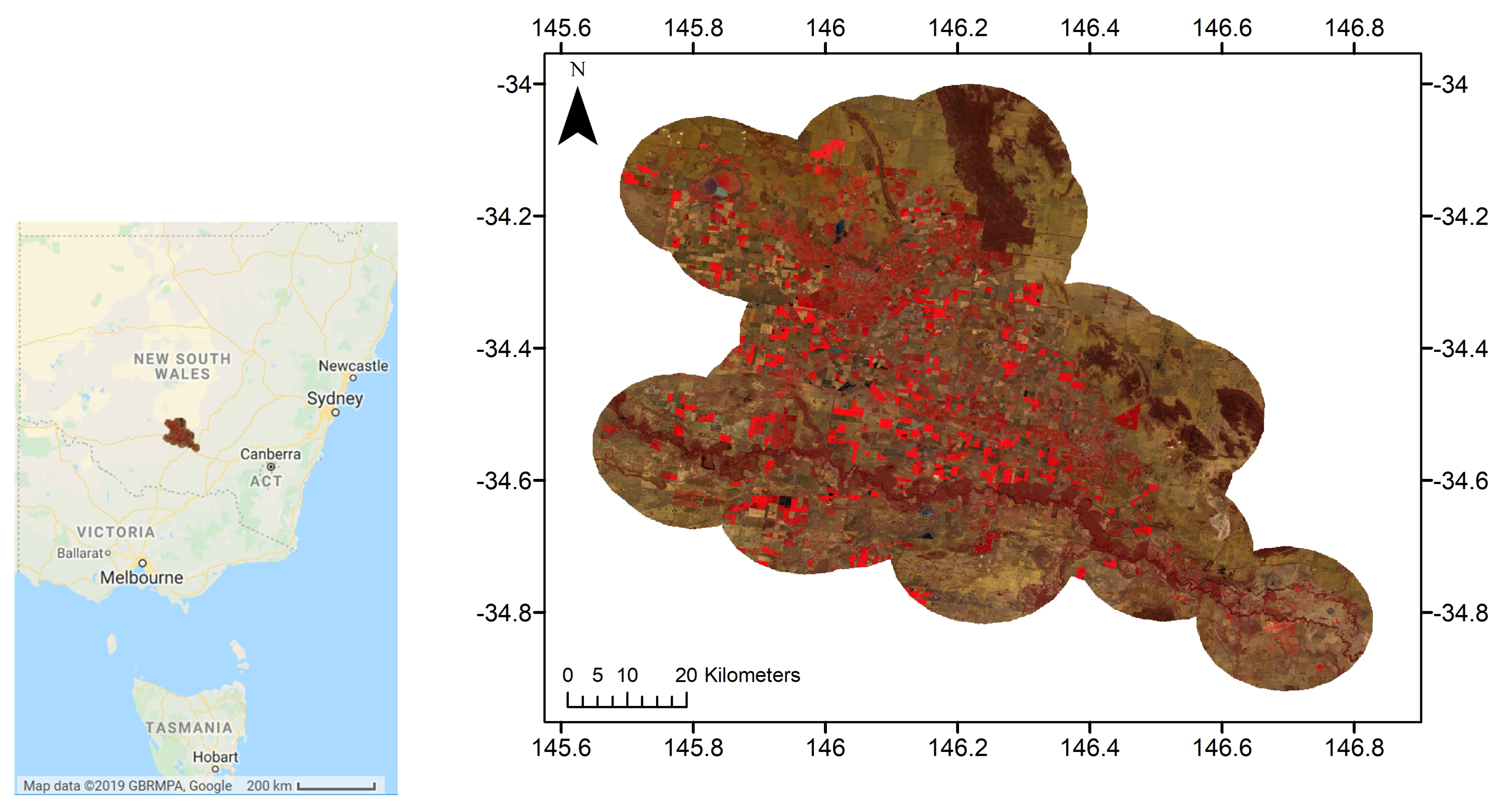
2.1. Study Area

This study focused on the area surrounding the Leeton and Griffith townships within the Riverina, NSW, Australia. Irrigated agriculture is a major industry in these areas, with irrigation water supplied from the Murrumbidgee River. Crops can be classified as perennial or annual. Annual crops include cotton, rice and maize grown in the summer; and canola, wheat and barley grown in the winter. Growers sometimes rotate summer and winter crops on their fields and may choose to leave annual cropping paddocks fallow. Perennial crops grown in the area include citrus, wine grapes, almonds among others.

A false color map of the analysis area is shown in Figure 1, using a mosaic of January 2019 Sentinel-2 images. The bounds of the analysis area was generated by buffering the training points (discussed below) by 12 km. The total analysis area is approximately 6200 km².

2.2. Definitions of the Twelve Land Cover Classes

The main aim of this study was to identify perennial crops across the study area. The definitions of the twelve classes we used are given in

Table 1. Definitions of the nine perennial crop classes and three remaining classes.

Group	Class	Notes
Perennial crops	Citrus	Includes common oranges (mainly the Valencia) and navel oranges Citrus sinensis. There are also some Grapefruit Citrus paradisi, Lemon Citrus limon and Mandarin Citrus reticulata orchards.
	Almond	Prunus dulcis.
	Cherry	Prunus avium.
	Plum	Prunus domestica, which in this area are mainly used to produce dried prunes.
	Stonefruit	Other stonefruit, which includes small areas of Nectarines Prunus persica var. nucipersica, Peaches Prunus persica and Apricots Prunus armeniaca.
	Olive	Olea europaea.
	Hazelnut	Corylus avellana.
	Walnut	Juglans regia.
	Vineyard	Vitis vinifera, mainly used to grow grapes for wine production in this area.
Other areas	Annual	Annual crops, which includes those mainly grown over the summer (such as rice, cotton and maize) and those grown over the winter (such as barley, canola and wheat) as well as melons and vegetables.
	Forest	Trees other than those used to produce a crop, such as native forest areas, mainly consisting of evergreen Eucalyptus.
	Other	All other areas, including water, buildings, grass and cropping areas not planted during the study year.

, separated into perennial cropping (9 classes) and other land cover types (3 classes).

Perennial plants are those which live for more than two years [35]. They include evergreen species (such as Citrus and Olive) and deciduous varieties (such as Almond and Plum). When classifying between vegetation land cover types, the number and granularity of classes must be decided. More classes may give better homogeneity within each class, but will result in less training data per class. We settled on nine perennial crop classes, separating out those most important for the area, and for which we could gather sufficient training data. Other areas were grouped into three classes, Annual, Forest and Other. The Annual class is heterogeneous, as it included winter and summer crops. The Other class is also heterogeneous, because of the wide range of land cover types it incorporates, including vegetation, water and built structures. This within-class heterogeneity is ameliorated by the use of K-means clustering, described in following sections.

2.3. Image Sources and Pre-Processing

This section describes the remote sensing imagery that was used and the methods of preprocessing it to obtain a single multi-band image ready for further analysis. Sentinel-1 (S1) synthetic aperture radar (SAR) and Sentinel-2 (S2) multispectral images from the ESA constellations [36] were accessed and processed in the Google Earth Engine (GEE) cloud environment [37]. The S1 SAR pixels had 10 m ground resolution, and the S2 multispectral pixels had 10 or 20 m resolution depending on the band (see

Table 2. Sentinel-1 (S1) and Sentinel-2 (S2) bands. NDVI = (NIR − R)/(NIR + R) was also computed at 10 m resolution, and NDVI together with the S2(4) bands formed the S2(5) grouping.

Grouping	Band	Abbreviation	Approx. Band Center	Resolution (m)
S1(2)	VV	VV	5.4 GHz	10
	VH	VH	5.4 GHz	10
S2(4)	Blue	B	490 nm	10
	Green	G	560 nm	10
	Red	R	660 nm	10
	Near infrared	NIR	830 nm	10
S2(10) (includes S2(4))	Red edge 1	RE1	700 nm	20
	Red edge 2	RE2	740 nm	20
	Red edge 3	RE3	780 nm	20
	Near infrared narrowband	NIRN	860 nm	20
	Short wave infrared 1	SWIR1	1610 nm	20
	Short wave infrared 2	SWIR2	2200 nm	20

). The bands were grouped into S1(2) for the SAR bands, S2(4) for the 10 m resolution S2 bands, and S2(10) for all S2 bands. S2(5) adds the normalized difference vegetation index (NDVI) to the four S2(4) bands. All images over the study area from the start of May 2018 to the end of April 2019 were used.

The time series of S1 and S2 images were pre-processed as shown in Figure 2. For both S1 and S2 image sets, monthly mosaics were generated, and these were then combined into a single multi-band image.

For the Sentinel-2 (S2) images, the process to generate the monthly mosaics was:

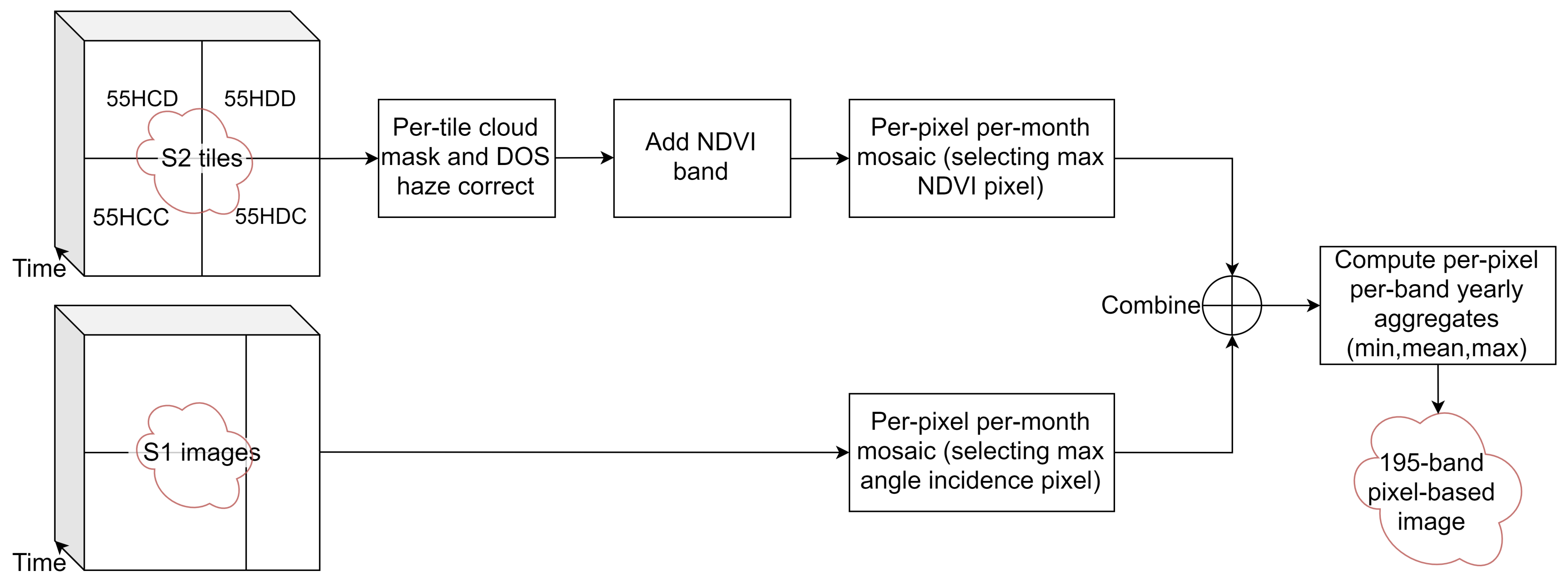
• The four image tiles intersecting with the area of interest (55HCD, 55HDD, 55HCC and 55HDC) from 1 May 2018 to 30 April 2019 were collected. This included 579 tiles, giving an average of 48 tiles per month, or 12 acquisition dates per month.
• Clouds in each tile were masked using the quality band metadata.
• Dark Object Subtraction (DOS) haze correction [38] was applied to each tile to obtain psuedo surface reflectance values.
• NDVI = (NIR − R)/(NIR + R) was computed.
• The four 10 m resolution bands, six 20 m resolution bands (see Table 2) and NDVI were selected, giving 11 bands per tile.
• A single mosaic was generated for each month. As multiple images are available for each month, the monthly images were generated using a quality mosaic method, selecting the image per-pixel with the highest NDVI, similar to [39]. This produces twelve images, each with eleven bands.
• The bands were renamed with the band name followed by mosaic month with the format YYMM. For example, the NIR band from May 2018 was named NIR_1805. The twelve image mosaics were flattened into a single 12 month × 11 band = 132 band image.

A similar multi-band image is generated from the Sentinel-1 (S1) SAR data, using the radar backscattering coefficient bands VV and VH (vertical transmit polarisation with vertical and horizontal receive polarisation, respectively). A total of 91 images intersecting the study area were obtained, giving between 7–8 images per month. Monthly mosaics were generated on a pixel-by-pixel basis, selecting the image per-pixel with the greatest incidence angle, in order to use acquisitions with similar imaging geometries for the mosaics. The resulting range of incidence angles for all the mosaics was 34.1–45.1${}^{\circ }$. The image collection was flattened to a single 24-band image with band names such as VV_1805, resulting in a single 12 month × 2 band = 24 band image.

Per-pixel statistics (minimum, mean and maximum) across the twelve months were computed for each of the bands of the S1 and S2 images. These aggregate bands facilitated assessment of the classified map accuracy achievable using these three summary statistics bands (for example for the NIR band NIR_min, NIR_mean, NIR_max), compared to the twelve monthly bands, which characterize phenological change (for example NIR_1805, NIR_1806,…, NIR_1904). These aggregate bands were added to the monthly mosaics, and the resulting total number of bands in the final image was (S1_bands + S2_bands) × (months + statistics) = (2 + 11) × (12 + 3) = 195 bands. Not all bands were used in all classifications, rather numerous subsets of bands were selected to asses the relative accuracy using each of these band combinations.

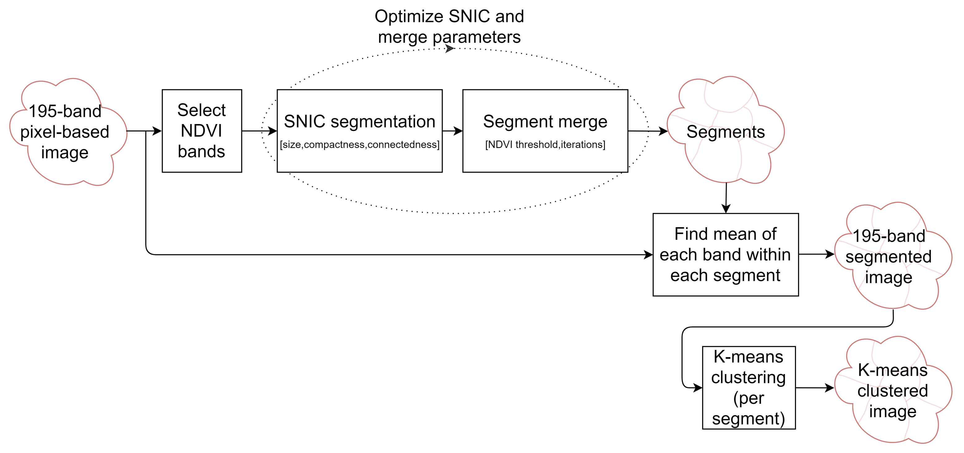
2.4. Segmentation Optimization for Object-Based Image Analysis

In this section, we describe the methods used to segment the pixel-based image. This included optimization of segmentation algorithm parameters, and generation of the final segments used in following analysis. The superpixel non-iterative clustering (SNIC) technique [40] as implemented in GEE [37] was used to spatially cluster pixels into objects (called segments throughout this paper) to facilitate object-based image analysis (OBIA). The algorithm grows segments around a grid of seeds (with seed spacing set by the size parameter), optimizing a measure combining spatial and spectral distances. The compactness parameter provides a tradeoff between square segments on one extreme (spatial compactness), and close boundary adherence on the other (spectral compactness).

SNIC was applied to the monthly NDVI mosaic bands (NDVI_1805, NDVI_1806,…, NDVI_1904) as shown in Figure 3. To find parameters for the SNIC algorithm that optimally delineate typical fields, SNIC was first run over a sub-section of the study area, sweeping the algorithm parameters including size (from 20 to 100 in steps of 20) and compactness (0, 0.1, 0.2, 0.4 and 0.8).

Following this, a merging algorithm was used to group spectrally similar segments together, applied either 0, 1 or 2 times. Adjacent segments were merged if all 12 month NDVIs were within a threshold (0.05 and 0.1). These merging parameters are denoted in the results section using terminology such as “2 $\times \Delta <0.05$”, meaning two iterations of merging with an NDVI threshold of 0.05. The sweeps of SNIC and merging parameters generated a total of 125 rasters of segments, with an identification number assigned to each segment.

Seventy-five polygon geometries were drawn, each outlining a homogeneous field. They were selected to include a range of crop types, field shapes and field sizes. Their boundaries were defined by inspecting the very high resolution Google basemap from 2019. The average size of these fields was 3 hectares and the average perimeter was 680 m. These were used as a basis for assessing the accuracy of each of the 125 segmentation and merge parameter sets in delineating the fields accurately. An example is shown in Figure 4. The segments that intercepted the 75 geometries (internally buffered by 10 m to avoid issues with geo-location errors between S2 and basemap imagery) were selected, called the intercepting segments.

Two metrics were evaluated for each parameter set:

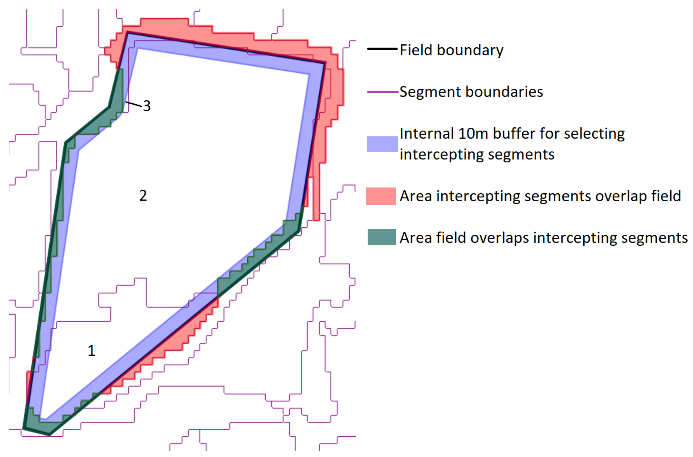
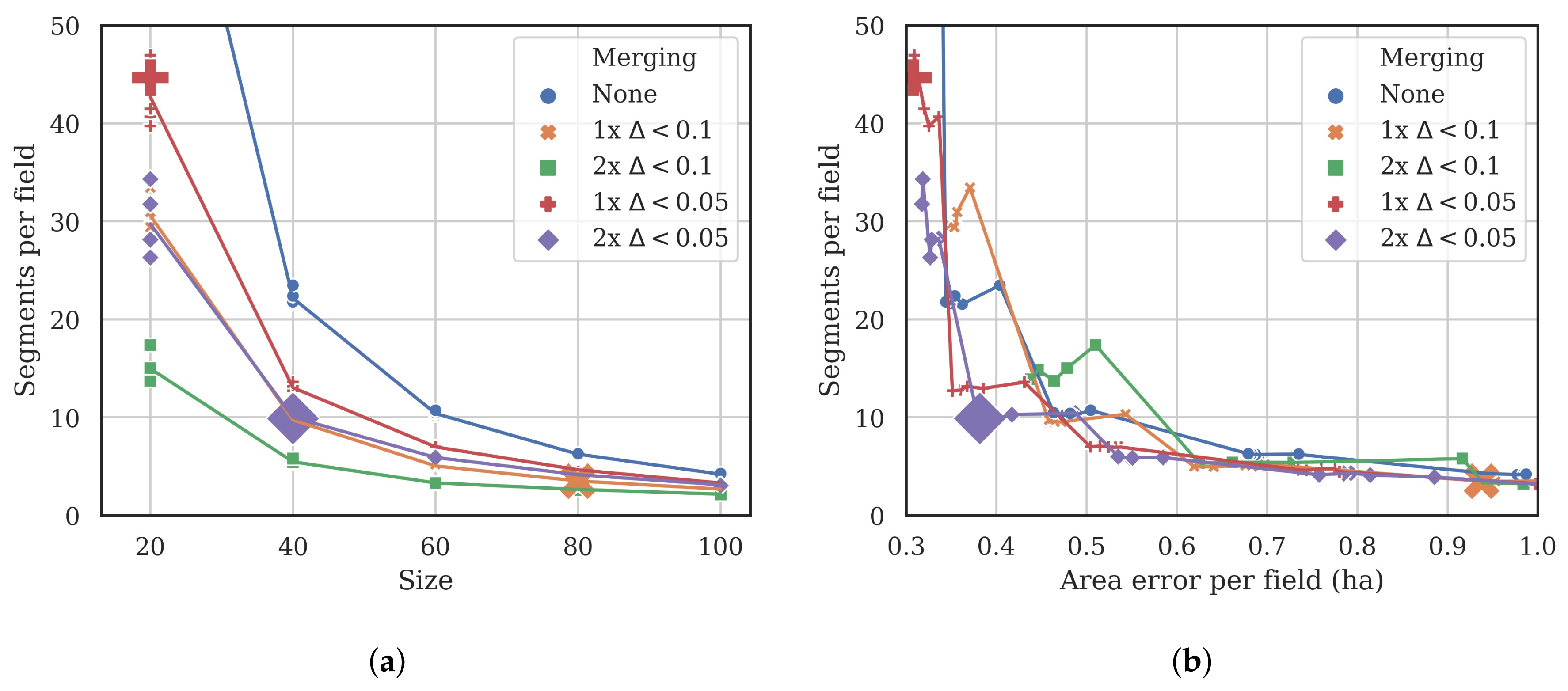
• The total area error, which is the sum of two components:
  • Omission errors, that is the area of the test geometries that are not covered by the intercepting segments (green area in Figure 4).
  • Commission errors, that is the area of the intercepting segments that overlap the test geometries (red area in the figure).
• The total number of segments intercepting the 75 test objects (3 in the example shown in Figure 4).

A smaller the total area error indicates more accurate field delineation. However, there is a tradeoff between the number of segments and area error. These tradeoffs were considered when selecting the optimal parameters.

Once the optimal parameter set was chosen, the SNIC and merging algorithms were run over the entire study area, generating the segments used in the classifications (“Segments” in Figure 3). The 195-band pixel-based image was then segmented using these object boundaries, with the mean values of each of the bands per segment computed (“195-band segmented image” in Figure 3).

K-means clustering was run on the monthly NDVI bands of the segmented image, with k = $[2,3,4,6,10,20,40,80,160]$ clusters. These clusters are used to filter training point outliers and to classify some Other and Annual areas of the final maps, discussed further below.

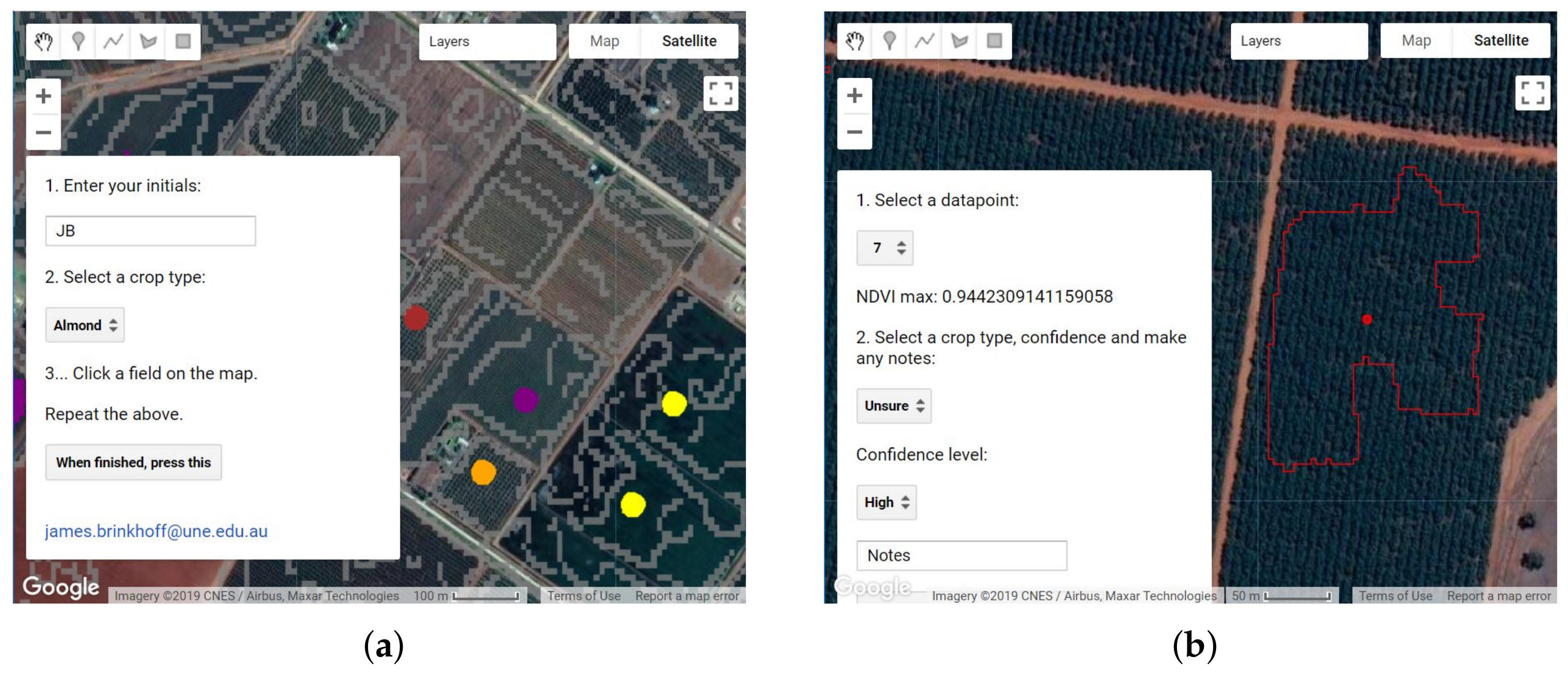
2.5. Training Data Collection and Cleaning

This section outlines the methods to obtain and clean the labelled training data for map classification. A GEE web application was developed, shown in Figure 5a. It displayed the segment boundaries overlaid on a high-resolution basemap. The twelve classes [Almond, Annual, Cherry, Citrus, Forest, Hazelnut, Olive, Other, Plum, Stonefruit, Vineyard, Walnut] were selectable in a drop-down menu. We enlisted the services of local area agriculture experts with detailed knowledge of crop types and locations. They entered crop types and associated locations on the map. These points were then downloaded as a GeoJSON file, with each record containing location and crop type. All of the generated training data files were merged. This yielded the “Training points” table in Figure 6 with 2005 points.

The segmented image was sampled at all of the training points. This generated another 2005 row table, with each row containing the class, location, means of all the image bands and K-means values (“Samples” in Figure 6).

All sample features were standardized to have a mean of 0, and standard deviation of 1. This improves classification accuracy using the SVM algorithm when features have differing numeric ranges [41]. This was the case with the features used in this work, as the S1 backscatter coefficients are much smaller than the S2 reflectances.

The K-means cluster values were used to identify and filter anomalous points from the training data. These anomalous points included:

• Points marking new perennial plantings, where the canopy cover is small relative to the row and tree spacing. The 10 m Sentinel pixels contain more soil than canopy in these areas, and thus, are not able to classify these areas accurately.
• Points marking annual cropping areas that were fallow in the study year.

In both these cases, the NDVI is low compared to the mean NDVI of the respective class. We analyzed the maximum NDVI per class over the year, and the timing of this maximum, per class and per K-means cluster. We found that the K-means clusters with k = 3 could effectively identify these training points with very low vegetation (cluster 1). It could also identify areas used to grow an annual crop over the winter (cluster 2). These points were removed from the samples, giving the “Filtered samples” table with 1386 rows remaining, shown in Figure 6.

Areas of the map belonging to these low vegetation and winter vegetation K-means clusters (1 and 2) were classified as Other and Annual, respectively, so that part of the classified maps was derived using unsupervised classification. Following this, supervised classification was run on points and areas of the map belonging to the remaining K-means cluster (0), which contained the nine perennial crops, forest areas, summer annual cropping areas and other vegetation. The classification methodoloy is described further in the following section.

2.6. Classification

This section describes the methods used to select classifier algorithms and optimize their parameters, to then use these classifiers to generate land cover maps, and finally to assess the accuracy of these maps.

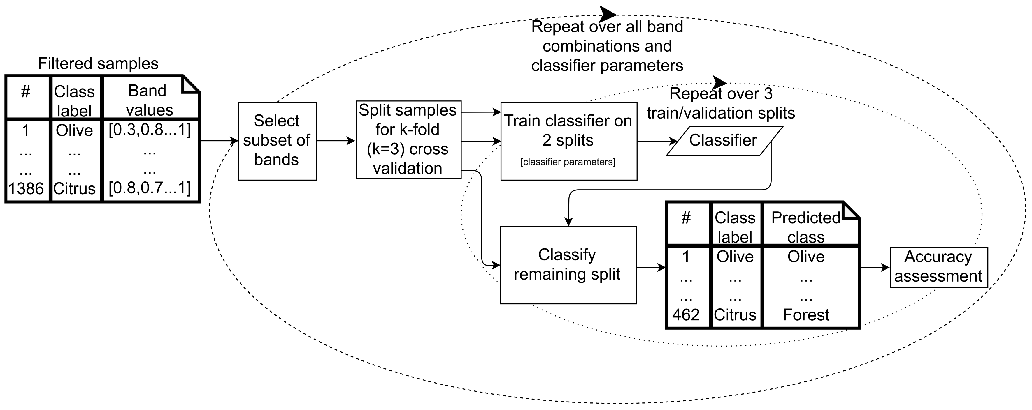
2.6.1. Supervised Classifier Optimization

Supervised classifiers were trained with the filtered samples dataset (Figure 6). The classification algorithms available in GEE that were assessed were:

• Classification and regression tree (CART), a decision tree algorithm, which classifies data points using successive decisions based on feature values.
• Random forest (RF), which uses the average of multiple decision trees, each trained on different subsets of training data and features, to arrive at a classification for each data point.
• Support vector machine (SVM), which classifies data points based on finding hyperplanes (surfaces defined by combinations of input features) that optimally separate the classes based on training data. SVM with linear and radial basis function (RBF) kernels were assessed.

A number of band combinations were trialled. We generated maps for a subset of these, which are shown in

Table 3. Band combinations used in supervised classification. TS = time series. Agg = aggregate bands computed per pixel over the twelve months. Months are indicated as YYMM (e.g., 1805 is May 2018).

Designation	Bands	Months	Features
S1(2) TS	VV, VH	1805, 1806, …, 1904	24
S2(4) 1 month	B, G, R, NIR	1806	4
S2(5) 1 month	B, G, R, NIR, NDVI	1806	5
S2(10) 1 month	B, G, R, NIR, RE1, RE2, RE3, NIRN, SWIR1, SWIR2	1806	10
S2(5) 2 month	B, G, R, NIR, NDVI	1809, 1810	10
NDVI TS	NDVI	1805, 1806, …, 1904	12
S2(4) TS	B, G, R, NIR	1805, 1806, …, 1904	48
S2(10) TS	B, G, R, NIR, RE1, RE2, RE3, NIRN, SWIR1, SWIR2	1805, 1806, …, 1904	120
S2(10) + S1(2) Agg	B, G, R, NIR, RE1, RE2, RE3, NIRN, SWIR1, SWIR2, VV, VH	Min, Mean, Max	36
S2(10) + S1(2) TS	B, G, R, NIR, RE1, RE2, RE3, NIRN, SWIR1, SWIR2, VV, VH	1805, 1806, …, 1904	144

.

The parameters for each classification algorithm and band combination were optimized using the methodology is shown in Figure 7. The samples were split randomly into three groups. K-fold cross validation with k = 3 was then applied, training each classifier on 2/3 of the data, and validating on the remaining 1/3, repeating for the three combinations of training and validation data. The overall accuracy (correctly classified points divided by the total number of points) on the validation samples, and the mean of the overall accuracies over the three folds, were computed. The optimal classifier parameters were selected for each band combination. These classifier tuning parameters were then used while training the classifiers with the entire filtered training sample dataset. These final classifiers were then used in classified map generation.

Rows 2–4 of Table 3 refer to using only one month’s multispectral image with a range of spectral bands. Images from all single months were investigated and the ones giving the highest accuracy were chosen. Similarly, row 5 of Table 3 refers to the optimum combination of images from two months, chosen by assessing the accuracy of all possible combinations. The purpose of this was to find the optimum month/months to acquire imagery in the case that only one/two month’s data is available due to cost, cloud cover or other restrictions.

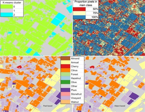
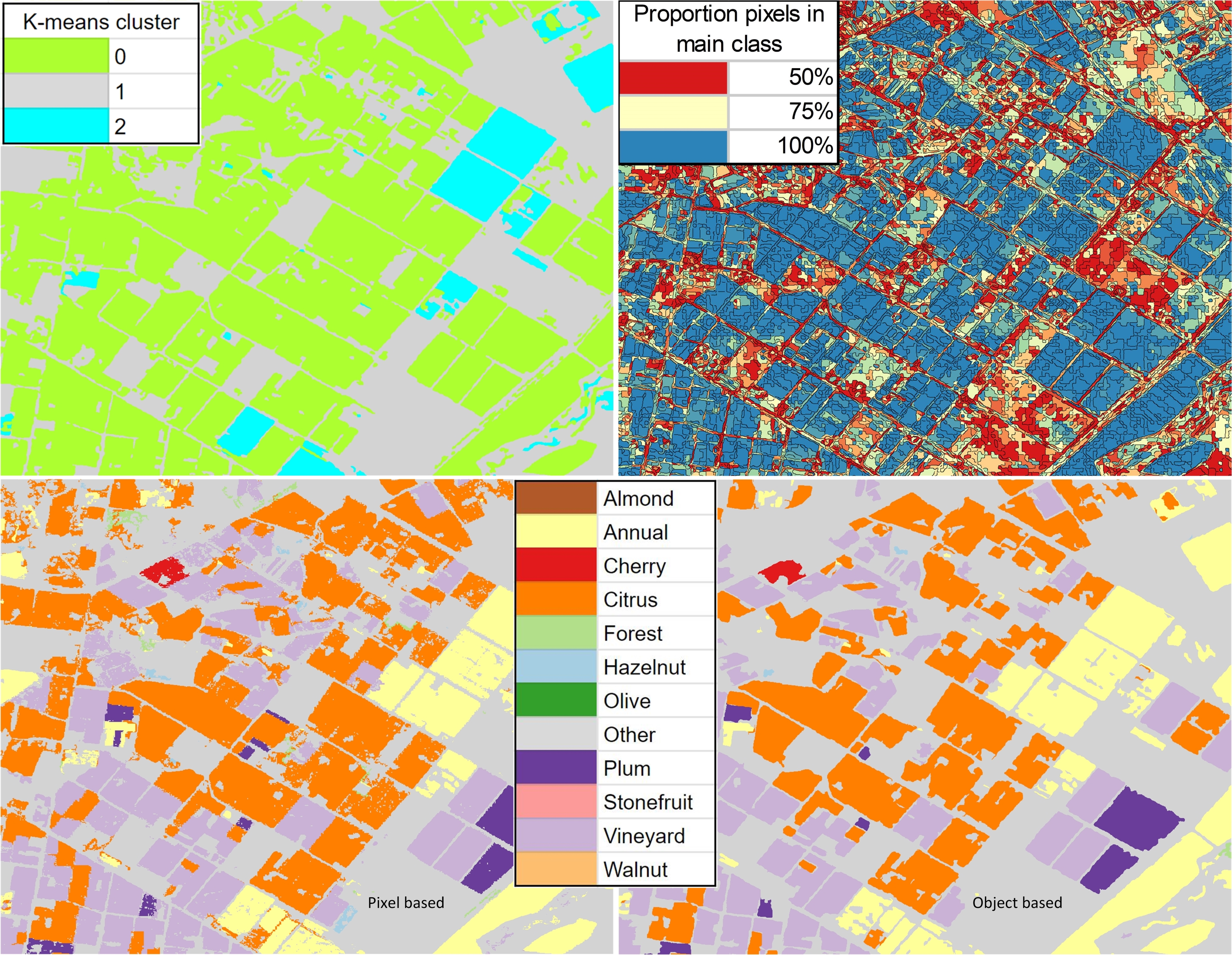
2.6.2. Classified Map Generation

Having determined the optimum classification algorithm and parameters of that algorithm for each band combination in Table 3, this section describes the method used to apply the classifiers over the whole study area to generate the land cover maps. The methodologies adopted are depicted in Figure 8.

First, as introduced above in Section 2.5, the K-means unsupervised classification image with k = 3 was used to set areas belonging to cluster 1 (which characterised low vegetation) to the Other class, and areas of the map the belonged to cluster 2 (which characterised dominant winter growth) were assigned to the Annual class.

Supervised classification was used to classify the remaining area of the map (belonging to K-means cluster 0), which included perennial crops and forest areas, summer annual crops and other vegetation. The SVM classifier with RBF kernel was used, as this produced higher accuracies than the other algorithms discussed above in Section 2.6.1. After the classifiers were trained on the K-means filtered samples (see Section 2.5), the classifiers were then run on the pixels or segments of the respective yearly S1 + S2 image. A number of strategies for generating the classified map were trialled, with the final map indicated by the filled red map symbols in Figure 8:

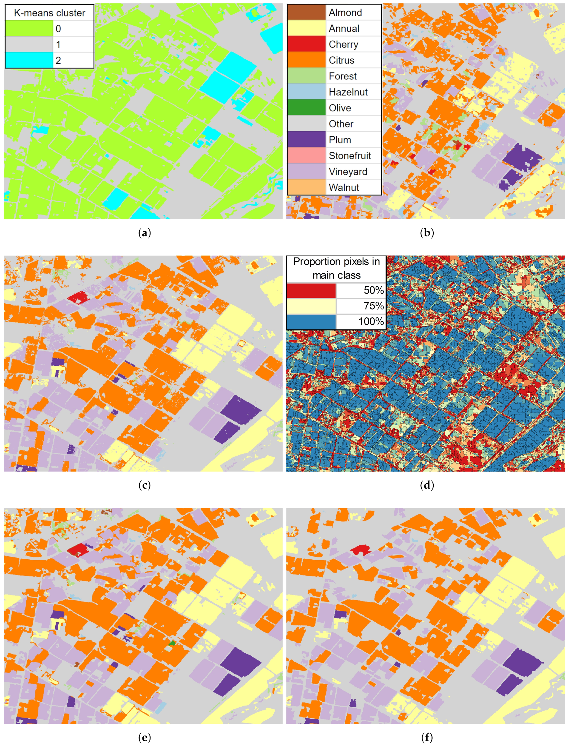
• The classifier was run pixel-by-pixel on the un-segmented original image, producing a pixel-based classified map.
• The classifier was run segment-by-segment on the segmented image, producing an object-based map.
• The pixel-based classified map was transformed into an object-based map by finding the majority pixel class within each segment, producing the refined object-based map.

The third procedure is similar to the object-based post-classification refinement (OBPR) in [42]. The procedure has the advantage that the proportion of pixels assigned to each class within each segment can be analyzed, to give a measure of the certainty the segment belongs to the majority class. If 100% of the pixels within a segment belong to a single class, it is likely that is the correct classification for the segment. However, as the proportion of pixels assigned to the majority class within a segment reduces, (i.e., a segment contains mixed pixels) there is less certainty that the majority class is the correct classification.

We used a procedure based on analysis of this proportion of pixels belonging to the majority class within each segment to optimize the tradeoff between producer and user accuracies [41]. A threshold was set, and a segment was assigned to the Other class if the proportion was below the threshold. A higher threshold will give greater certainty that the segment that is classified as belonging to a particular class does actually belong to that class, and thus a higher users’ accuracy, but a higher threshold will result in some segments being incorrectly classified as Other because of mixed pixels within the segment, thereby reducing the producers’ accuracy. On the other hand, a lower threshold will result in a higher producers’ accuracy, as no segments will be relegated to the Other class if there is some uncertainty, but this also gives a lower users’ accuracy, as this uncertainty due to mixed pixels will lead to segments being misclassified. Thus, a higher threshold increases users’ accuracy, but reduces producers’ accuracy and vice versa. The threshold can be chosen to balance the users and producers’ accuracies, or to optimize the most important accuracy measure for a given application.

Finally, adjacent segments belonging to the same class were merged. An area filter was applied, so that only contiguous segments with areas greater than 1 hectare were retained. Smaller island segments were classed as Other.

2.6.3. Classified Map Accuracy Assessment

This section details the methods used to assess the accuracy of the land cover maps. The training dataset was not used for this final accuracy assessment. Even if test points are held out of the training data for accuracy assessment, using these can result in an optimistic assessment [34]. This is because the training points are not randomised spatially, and bias is likely because they are self-generated by people. Instead, we used a random sampling scheme. Segments over the whole study area were randomly chosen, stratified according to classes from an early version of a classified map. An average of 28 segments for each of the classes were assessed, giving a total of 341 random validation points.

A further GEE web application was deployed, that displayed each of these randomly selected validation segments one by one. It also showed the maximum NDVI for each segment over the year. A screenshot is shown in Figure 5b. Local experts with detailed crop type and location knowledge were again enlisted. They assigned a class to each validation segment, collaborating with others with more insight into particular areas where needed. This data was exported as a table, with each row containing the segment area, the expert’s chosen validation class and the segment identification number (used to find the classified map class to compare with the validation reference class).

The equations for OBIA accuracy assessment described in [33] were used to find the overall (OA), producers (PA), and users (UA) accuracies, both count-based and area-based. Area-based accuracy weights the accuracies based on validation segment areas, so that larger segments will have more impact on accuracy than smaller segments. The overall accuracy is:

$$OA=\frac{{\sum }_{i=1}^n{S}_i{\sum }_{j=1}^k{\alpha }_{ij}{\beta }_{ij}}{{\sum }_{i=1}^n{S}_i}$$

(1)

where n is the total number of segments, k is the number of classes, ${\alpha }_{ij}$ is 1 if the reference label for segment i is j and 0 otherwise, ${\beta }_{ij}$ is 1 if the map label for segment i is j. True classification of segment i is indicated by ${\sum }_{j=1}^k{\alpha }_{ij}{\beta }_{ij}$ = 1, where the reference and map classes for segment i are equal. For area-based metrics, $S_i$ is the area of segment i. For count-based metrics, $S_i$ is 1.

The producers’ accuracy indicates the probability that an object belonging to class j is correctly classified:

$$P{A}_j=\frac{{\sum }_{i=1}^n{S}_i{\alpha }_{ij}{\beta }_{ij}}{{\sum }_{i=1}^n{\alpha }_{ij}{S}_i}$$

(2)

The users’ accuracy indicates the probability that an object mapped as belonging to class j does actually belong to that class:

$$U{A}_j=\frac{{\sum }_{i=1}^n{S}_i{\alpha }_{ij}{\beta }_{ij}}{{\sum }_{i=1}^n{\beta }_{ij}{S}_i}$$

(3)

Another accuracy measure that is often quoted is the kappa coefficient. However, as noted in [34], this does not add significant information to thematic map assessment over the above accuracy metrics.

3. Results

3.1. Segmentation Optimization

The SNIC segmentation algorithm, followed by similar adjacent segment merging, was run over the test area. Segmentation accuracy metrics were computed for the 75 test field polygons using the methods described in Section 2.4. Figure 9 shows the area errors and number of segments per field as a function of the SNIC size parameter and adjacent segment merging settings. Multiple points per size are visible because the compactness parameter was also swept. There is a tradeoff between the area error and the number of segments. With larger size values, there are less segments per field, but the segments have more area error due to segments tending to overlap the field boundaries. Conversely, smaller sizes have less area errors as they conform more closely to field boundaries, but each field encompasses many segments.

The three larger points in Figure 9 were chosen to demonstrate the effect of the parameters, with results shown in

Table 4. Area error and number of segments per field geometry for selected sets of SNIC segmentation and merging paramters. The parameters in the middle row were chosen.

Size	Compactness	Merging	Area Error Per Field (ha)	Segments Per Field
20	0.4	1 × $\Delta <$0.05	0.31	44.65
40	0.4	2 × $\Delta <$0.05	0.38	9.88
80	0.2	1 × $\Delta <$0.1	0.94	3.48

. With size = 20, and merging segments once with NDVI merging threshold = 0.05, there were almost 45 segments per field (averaged over the 75 field geometries), and an average area error of 0.31 ha. On the other hand, with size = 80, and merging once with and NDVI threshold of 0.1, there were only 3.5 segments per field, but the area error was large at 0.94 ha per field.

As noted in [43], classification accuracy is better if an image is over-segmented rather than under-segmented. Adjacent segments with identical class are merged after classification. If the fields are under-segmented, multiple classes are present in each object, leading to mixed characteristics and class confusion. We chose parameters that produced approximately 10 segments per field, and an area error of 0.38 ha per field (the middle row of Table 4). The SNIC parameters were size = 40, compactness = 0.4, and merging twice with an NDVI threshold of 0.05. The entire study area was segmented using these parameters, and the resulting segments were used for all subsequent object-based image analysis.

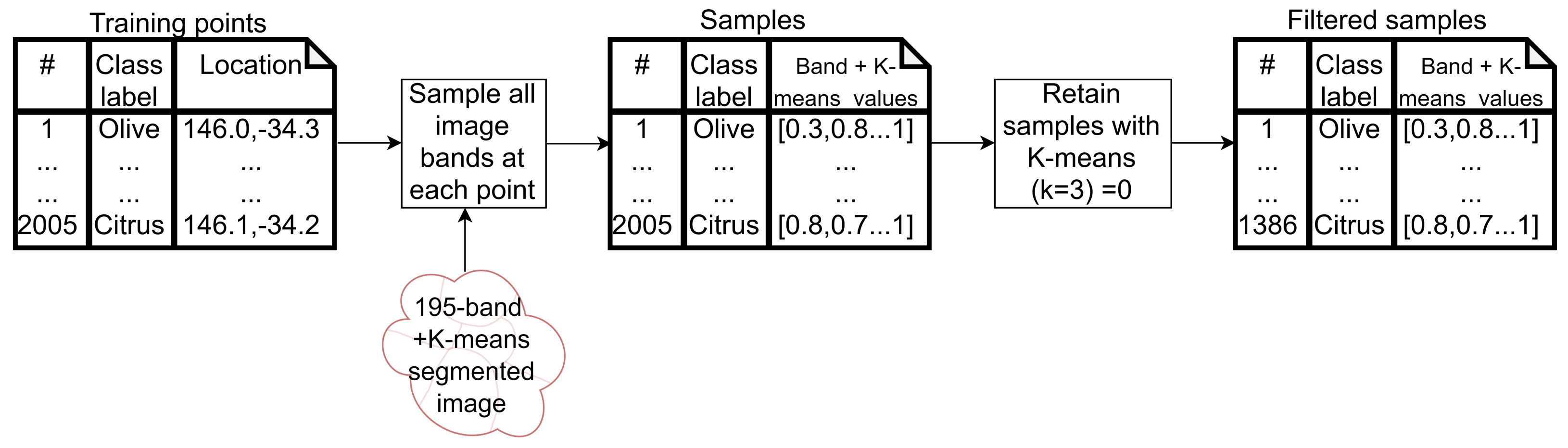
3.2. Training Data

A total of 2005 training points were gathered from field experts using the web app in Figure 5a. The number of training points per class are shown in Figure 10a, grouped by K-means (k = 3) cluster. The area devoted to growing cherries, olives and other stonefruit (nectarines, peaches and apricots) in the region is relatively small. There is only one major hazelnut farm and one major walnut farm. This resulted in an unequal distribution of training points per class.

Figure 10a shows how many points from each class belonged to each K-means (k = 3) cluster. Figure 10b shows the maximum NDVI per year for each of the clusters and groupings of classes. Finally, Figure 10c–e shows the NDVI over the year of each of the K-means clusters. From these, we made the following observations about each cluster:

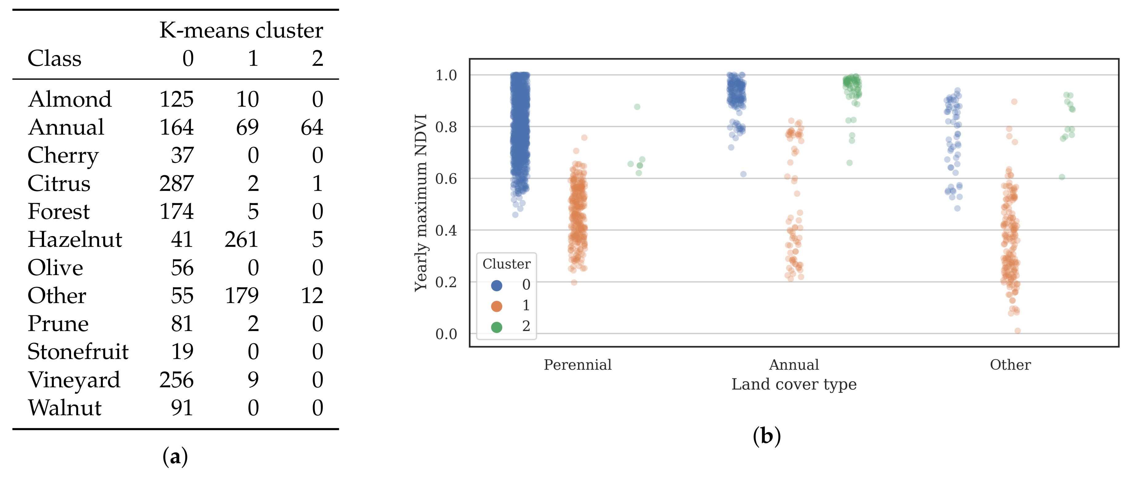
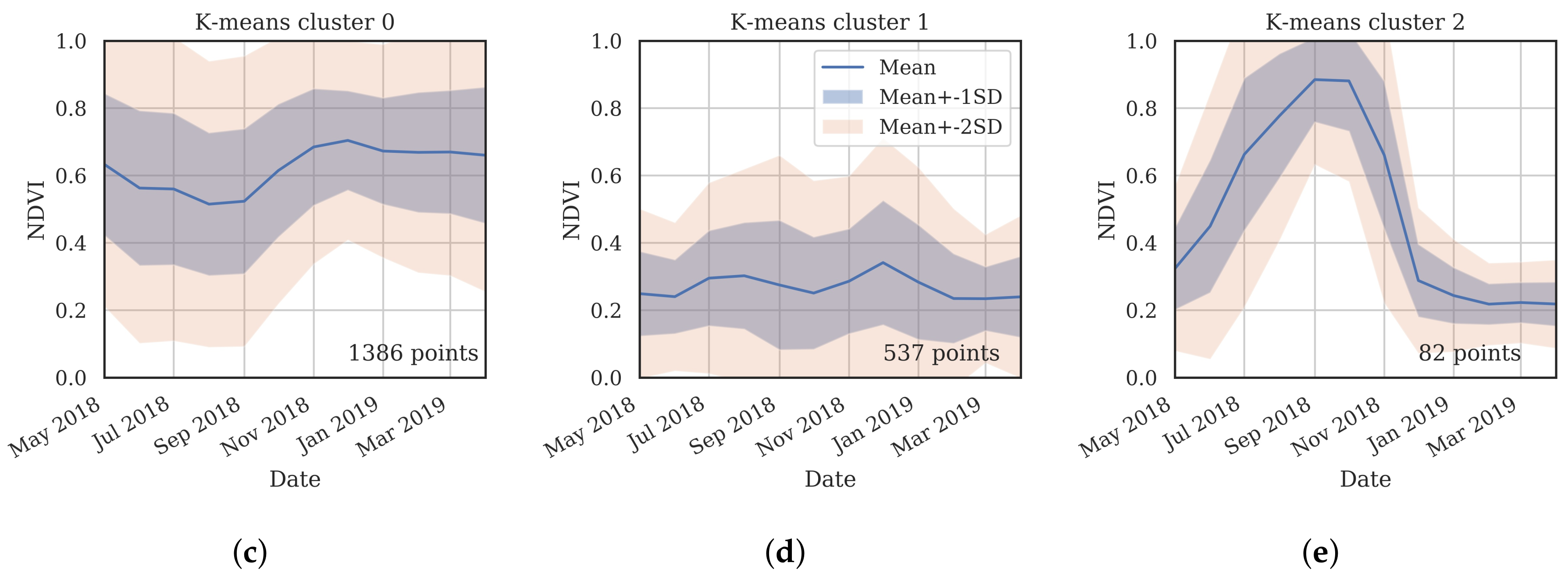
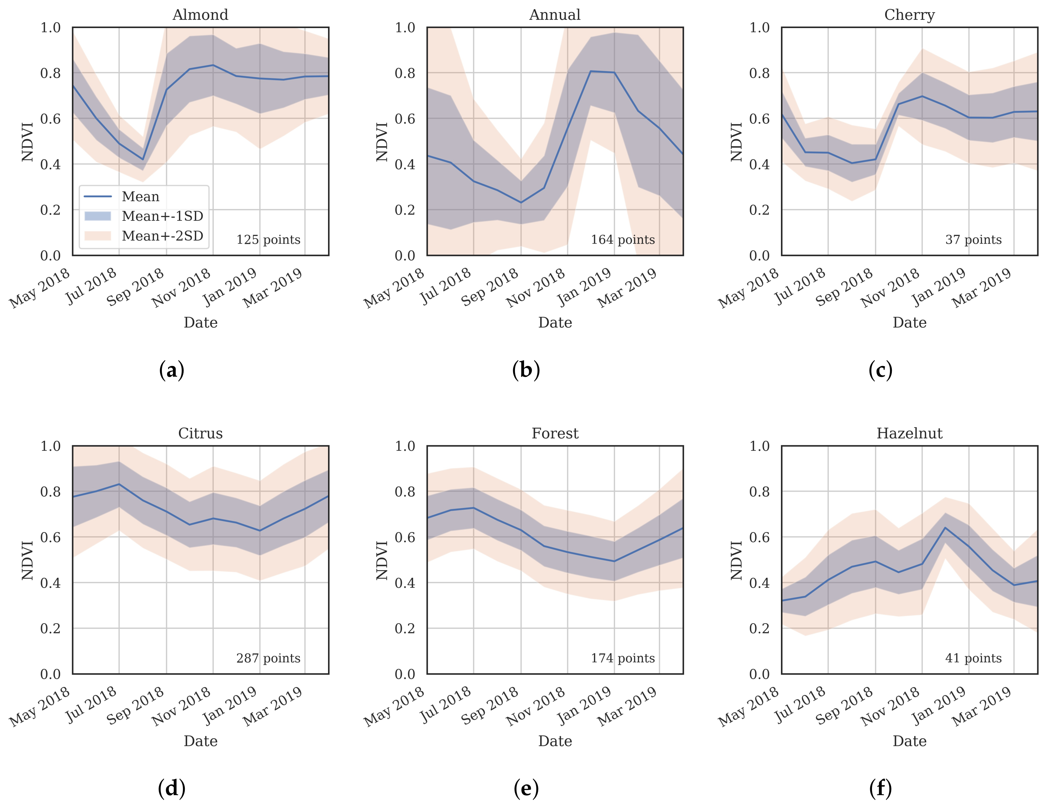
• Cluster 0 includes most of the perennial crop and Forest points, as well as the majority of the Annual points and some Other points. The NDVI time series shows that the cluster includes areas with dominant growth over the late spring to early autumn months (October to April) and areas with evergreen growth.
• Cluster 1 includes points with low NDVI, corresponding to areas with little vegetation. The Annual points in this cluster are annual cropping areas that were fallow in the study year. The perennial points in this cluster were young or very sparse plantings (which is the case in much of the Hazelnut growing area), with insufficient canopy to be detectable using the 10 m imagery. The majority of the Other points are in this cluster, corresponding to unplanted areas, built up areas and water bodies.
• Cluster 2 has high NDVI over the late winter to early spring months (July to November). This cluster is dominated by a significant number of Annual points. Therefore, this cluster identifies winter-grown annual crops.

These observations suggest a way of using the K-means clusters to both filter training points, and to assign classes to parts of the thematic maps. Areas belonging to K-means cluster 1 were assigned to the Other class, as these were areas without sufficient vegetation to be detectable by the 10 m resolution imagery. Cluster 2 was assigned to the Annual class as it identifies fields used for winter crops. Points belonging to clusters 1 and 2 could then be removed from the training data set.

Cluster 0 includes the perennial crops, annual crops grown over the summer, forest areas and other vegetation. 1386 of the 2005 training points belonged to this cluster and were used to train the supervised classifiers. These classifiers were then used to classify the map areas belonging to cluster 0. As seen in Figure 11, this provided greater homogeneity within the training points for Annual and Other classes, as areas with low vegetation or dominant winter growth were excluded. This increased homogeneity improves supervised classification of the cluster 0 areas.

Figure 11 shows the NDVI values per month for the 12 classes, which were derived from sampling the bands of the segmented S1 + S2 image at each of the training data points within the K-means cluster 0. The mean shows the general trend of the annual NDVI variation of each class, and the ±1 and 2 standard deviations indicate the within-class variability. Some classes have quite distinct characteristics, for example Walnut with its high and constant NDVI during its green phase, and sudden drop to dormancy in June. This contributes to high classification accuracy. On the other hand, the characteristics of other classes quite similar, for example the evergreen Olive, Citrus and Forest classes. Therefore, it may be difficult for a classifier to separate these classes based on using a time series of NDVI alone. However, the final classification included the time series of all reflectance bands, as well as the Sentinel-1 radar backscatter coefficients, which provides more features to distinguish each class.

3.3. Classifier Optimization Using the Filtered Samples

Classification accuracy using k-fold cross-validation with 3 folds was assessed on the samples with four classifier algorithms and many combinations of S1 and S2 bands (Figure 7). The most important parameters for each classifier were swept to optimize accuracy per band combination. The best overall accuracy for the CART classifier was 84.8%, while the RF classifier achieved 93.3%. The SVM classifier with RBF kernel had the highest accuracy of 97.7%, with the best combination of input features being all time series bands over the 12 months (S2(10) + S1(2) TS). The SVM classifier with RBF kernel produced higher accuracies than the other classifiers for all trialled band combinations (Table 3). Most of the following results therefore are for the SVM classifier with RBF kernel. The optimal SVM gamma and cost for each band combination were determined using cross-validation (see Section 2.6.1), and subsequently used to generate classified maps.

Future work may involve using higher resolution imagery, which comes at a cost and therefore obtaining an image per month may not be affordable. To investigate the best months to acquire such images, we assessed the accuracy using a single month of S2(5) multi-spectral data, and all combinations of two months of multi-spectral data. The accuracy of all combinations from each of these is shown in Figure 12. We note that the accuracies quoted in this section are assessed using classification of the filtered samples. Assessment of map accuracy using a random selection of segments is provided in following sections. For a single multispectral image, the June image gave the best accuracy of 80.4%. November to April images gave the lowest accuracies, which is the period were most classes exhibited high NDVI (Figure 11). The best combination of two months was September and October, which yielded an accuracy of 92.5%.

3.4. Classified Map Generation and Comparison

Using the optimum classifier parameters (found using the method described in the previous section), numerous classified maps of the entire study area were produced using input features composed of the band combinations in Table 3. A 33 km² portion of some of these are shown in Figure 13. Figure 13a shows the K-means (k = 3) clusters. In all the maps, clusters 1 and 2 are classified as Other and Annual, respectively, and cluster 0 is classified using SVM with RBF kernel supervised classification, unless otherwise noted.

To assess map accuracy, validation segments were randomly selected from the entire study area. The goal was to stratify these based on classified map class, with approximately 30 segments per class. However, this stratification was performed on an earlier and less accurate version of the map, so there was variation in the number of segments per mapped class. In total, 341 segments with a total area of 344 ha were validated by field experts using the web application shown in Figure 5b. Validation segment locations are shown on the final classified map below. Maps produced by directly classifying the segmented image (“195-band segmented image” producing the “Object-based classified map” in Figure 8) had overall accuracies shown in Figure 14 and described in the following paragraphs.

Figure 13b shows object-based classification using only the S1 radar bands S1(2) TS. This achieved an overall accuracy (OA) of 67.7% against the validation segments.

We investigated maps generated using the best single month multispectral image (June). Adding NDVI to the four 10 m resolution bands (B, G, R, NIR) did not improve accuracy, having accuracies of 71.6% and 72.1%. However, including all ten S2 bands improved the accuracy to 77.4%. This demonstrates the usefulness of increased spectral resolution in classifying crops. Using the two best months (September and October) with 5 bands improved the accuracy to 78%. This demonstrates that temporal information may be more important than spectral resolution for this kind of classification problem, as S2(10) June and S2(5) Sept + Oct both have ten features but the latter has slightly better accuracy.

The twelve month time series of only NDVI also had OA = 78%. Using the time series of 10 m S2 bands (S2(4) TS) had OA = 79.2%, while incorporating the 20 meter resolution bands (S2(10) TS) improved the accuracy to 83%. The map generated using all aggregate bands (S2(10) + S1(2) Agg) had OA = 83.3%, only slightly less accurate than using all time series bands (S2(10) + S1(2) TS), which achieved the highest accuracy of all the object-based maps of 84.2%. For the same bands, but without the K-means filtering and unsupervised classification of clusters 1 and 2, the accuracy dropped to 76.2%, demonstrating the improvement of the combined unsupervised-supervised classification technique we adopted. The maps generated using the CART and RF classifiers with the same bands had lower accuracies than the SVM map, with OA = 66% and 74.5%, respectively.

Pixel based classification using all time series bands S2(10) + S1(2) TS is shown in Figure 13c. “Salt-and-pepper” effects are evident, but the map is still relatively interpretable. The proportion of pixels belonging to the majority class within each segment was calculated, and is shown in Figure 13d. Generally, well-defined agricultural fields have a high proportion of the majority class (shown as blue), leading to more certainty in their correct classification. Other areas such as buildings, roads and transition between fields have a lower proportion of pixels belonging to the majority class (shown as red).

We now consider the refined object-based maps (Figure 8). These were generated by selecting the majority pixel class within each segment. Then segments with proportion of pixels belonging to the majority class less than a set threshold were classified as Other. The tradeoff between average users (UA) and producers (PA) accuracies as a function of the proportion threshold is shown in Figure 15, with accuracies assessed against the random validation segments. The users’ accuracy for the map with threshold = 0% (simple selection of majority pixel class per segment) is significantly lower than the producers’ accuracy. As the threshold for the proportion of pixels belonging to the majority class increases, the users’ accuracy increases and producers’ accuracy decreases as described in Section 2.6.2. Maps with the threshold set to 0% and 80% are shown in Figure 13e,f, respectively. The threshold = 0% map has an overall accuracy of 85%, and there are some islands belonging to unexpected classes in the image, resulting from segments which have pixels with mixed characteristics. The threshold = 80% map is cleaner but has a lower overall accuracy of 79.2%. For the final map, we settled on a threshold of 60%, with OA = 84.8%, average UA of 86.4% and average PA of 88.7%.

Final Map and Accuracy Assessment

The final map was generated using the SVM classifier with RBF kernel, cost = 10, gamma = 0.01, and all 144 time series bands (S2(10) + S1(2) TS) as input features. Pixel-based classification was performed, followed by converting to a refined object-based map by finding the majority pixel class within each segment, and setting the class to Other if the proportion of majority pixels was less than the threshold of 60%. The classified map is shown in Figure 16.

The confusion matrix for the count-based accuracy assessment is given in Figure 17a. The area-based confusion matrix is shown in Figure 17b. The overall count-based accuracy is 84.8%, and area-based accuracy is 90.9%. The average area of the correctly and incorrectly classified segments is 1.1 and 0.6 ha, respectively, which is a reason for the higher accuracy of the area-based accuracy compared to count-based accuracy.

Analyzing the count-based accuracies, three out of the nine perennial crop classes had both UA and PA higher than 90%, and six of the nine had both UA and PA higher than 80%. Walnut had UA and PA close to 100% possibly because of its distinctive phenology (Figure 11l), as did Stonefruit though that class had only 5 validation segments. The classes with either UA or PA lower than 80% were Citrus (UA = 71%), Olive (UA = PA = 78%) and Hazelnut (UA = 63%). Hazelnut was concentrated in one area, and had quite low NDVI due to low canopy cover, which can be seen clearly on the high resolution base map. Forest was classified as Olive and Citrus in a number of the validation segments, probably due to their similar phenology.

4. Discussion

This work investigates a number of object-based classification strategies for land cover mapping, applied particularly to identifying and distinguishing between perennial crops.

We used a simple object delineation method, which relied on over-segmenting fields in order to avoid classification errors due to mixed characteristics within large segments. Once the classified map was generated, the segments with the same class were merged. Other work has aimed to generate one segment per field, for example using line detection methods that aid in the identification of typical field boundaries [43]. Such advanced segmentation techniques could be combined with the classification methodologies we developed to generate improved maps.

We found unsupervised K-means clustering useful to complement supervised classification, similar to [15]. This was due to the training data including points with a wide range of vegetation states (for example very young perennial plantings and fallow annual fields), which the clustering was able to separate. The method of combining unsupervised and supervised classification improved accuracy by 8% compared to using supervised classification alone. Among the supervised classifiers we trialled, SVM with RBF kernel yielded higher accuracies than the CART, RF or SVM with linear kernel. The greater performance of SVM over RF when discriminating between many crop types with similar features was also noted in [13].

We found, in agreement with [16], that using a time series of all available reflectance bands gave better classification accuracy than a time series of a vegetation index (NDVI) alone. The addition of radar data to multispectral data improved accuracy by just over 1%. Using radar data alone produced an accuracy of 67.7%, lower than multispectral data. However, the use of radar alone may be useful in areas with frequent cloud cover, where obtaining a time series of multispectral imagery is not possible. Future investigation could involve a more detailed analysis of selecting the best pixels for S1 mosaic generation, for example taking account of irrigation status, which SAR imagery is sensitive to [44]. We also compared using the four S2 10 m resolution bands, to using the ten S2 10 and 20 m bands, with the additional bands improving accuracy by more than 4%. We simply stacked the 20 m bands with the 10 m bands, but it would be useful to investigate more detailed ways of combining bands, such as sharpening the lower resolution bands using higher resolution data [45].

We studied the accuracy of cases where only one or two image acquisitions in a season is possible, which may be the case for example if expensive higher resolution imagery is required. Surprisingly, only two images acquired at optimal months (September and October in this region) and with only 5 bands (B, G, R, NIR, NDVI) had a reasonably high overall accuracy of 78%, which was only 6.2% less accurate than the map classified using the full time series with 10 multispectral and 2 radar bands. September and October are months are when there is a significant change in the NDVI in many of the species as seen in Figure 11, due to leaf growth during spring, which is a probably reason for the combination of images from those months giving the highest accuracy. Using only a single image with four bands gave a much lower accuracy of 71.6%, and ten bands improved this to 77.4%. This is still lower accuracy than obtained using two months with only five bands. This demonstrates the importance of including some information on vegetation change over time. We also compared using yearly summary statistics (min, mean, max) to the full time series data. The aggregate data gave an accuracy of 83.3%, only 0.9% lower than using all time series bands. This may be useful in cases where computational power is insufficient to generate large maps, as there is little accuracy penalty in using only a quarter of the input features (36 features vs 144 features). Future research could also consider using only the most important features in classification, using the feature importance ranking produced by random forest for example [21].

Cross-validation accuracies when classifying the training data was very high, with more than 95% accuracy achieved with the SVM classifier using monthly mosaics of Sentinel-2 and Sentinel-1 data. We noted that this training data was generated manually, was not spatially randomized, and so may include bias. When accuracy was assessed against randomly generated validation segments over the whole study area, overall accuracy of the best map was 90.9% (area-based) and 84.8% (count-based). This demonstrates the importance of proper classified map accuracy assessment with randomly sampled verification points, as validation using training data with non-random locations gives an overly optimistic accuracy assessment [34].

Other authors have noted the difficulty of discriminating between tree species [17] even when time series data is used, due to similar phenology between species. We also noted the variation in plantings in the study area, with some new plantings, and some plantings with significant gaps between trees. These effects can lead to pixels with mixed spectral signatures at the 10 meter image resolution we used [26]. Higher resolution imagery would facilitate the use of texture-based features [46], which has been shown to improve the classification of perennial crops [19]. Vineyards, for example, have a very consistent texture, and tree crops are usually planted with crop-specific tree spacings [47]. Being able to recognize these characteristics could reduce reliance on spectral information, which suffers within-class variability due to management and vigour differences.

We note that the season we studied was atypical. 2018 rainfall was only 56% of the average for the region, and the annual temperature was 1.7 °C higher than average, while the January 2019 average temperature was almost 6 °C above average. Water market prices were rapidly rising due to lack of supply. These factors may have contributed to greater variability in within-class characteristics, due to management choices and environmental pressure. Future work should consider multiple seasons, acknowledging the increased requirement of training validation data due to the need to take account of perennial planting changes over larger time scales (due to abandoned fields, changed crop types or newly planted fields).

Current land use maps in this region are quite coarse spatially, have limited discrimination between perennial crops and are updated infrequently. Techniques and data such as those presented here will be a useful complementary source of information in intensive cropping areas, enabling regular updates and the mapping many perennial crops at a finer spatial resolution.

5. Conclusions

In this study, a land cover map encompassing an area of 6200 km² within the Riverina region in NSW, Australia, was produced, with a particular focus on locating perennial crops and differentiating between them. A time series of Sentinel-1 radar and Sentinel-2 multispectral images was used. Unsupervised K-means and supervised SVM classification were combined with object-based image analysis techniques to optimize accuracy. Overall accuracy with twelve classes was 84.8% for object count, and 90.9% when weighted by object area. This demonstrated the possibility of producing detailed land cover maps over intensive perennial cropping areas using a time series of medium resolution remote sensing images. Suggestions for improving the map were put forward, including the use of higher resolution imagery that would enable the derivation of textural features, and the use of more than a year of data in the time series to ameliorate the effects of seasonal conditions.

References

- Lesslie, R.; Barson, M.; Smith, J. Land use information for integrated natural resources management—A coordinated national mapping program for Australia. J. Land Use Sci. 2006, 1, 45–62. [Google Scholar] [CrossRef]
- Tang, Z.; Engel, B.A.; Pijanowski, B.C.; Lim, K.J. Forecasting land use change and its environmental impact at a watershed scale. J. Environ. Manag. 2005, 76, 35–45. [Google Scholar] [CrossRef] [PubMed]
- Verburg, P.H.; Schot, P.P.; Dijst, M.J.; Veldkamp, A. Land use change modelling: Current practice and research priorities. GeoJournal 2004, 61, 309–324. [Google Scholar] [CrossRef]
- Teluguntla, P.; Thenkabail, P.S.; Xiong, J.; Gumma, M.K.; Congalton, R.G.; Oliphant, A.; Poehnelt, J.; Yadav, K.; Rao, M.; Massey, R. Spectral matching techniques (SMTs) and automated cropland classification algorithms (ACCAs) for mapping croplands of Australia using MODIS 250-m time series (2000–2015) data. Int. J. Digit. Earth 2017, 10, 944–977. [Google Scholar] [CrossRef]
- Schauer, M.; Senay, G.B. Characterizing Crop Water Use Dynamics in the Central Valley of California Using Landsat-Derived Evapotranspiration. Remote Sens. 2019, 11, 1782. [Google Scholar] [CrossRef]
- Gumma, M.K.; Tsusaka, T.W.; Mohammed, I.; Chavula, G.; Ganga Rao, N.V.P.R.; Okori, P.; Ojiewo, C.O.; Varshney, R.; Siambi, M.; Whitbread, A. Monitoring Changes in the Cultivation of Pigeonpea and Groundnut in Malawi Using Time Series Satellite Imagery for Sustainable Food Systems. Remote Sens. 2019, 11, 1475. [Google Scholar] [CrossRef]
- Pfleeger, T.G.; Olszyk, D.; Burdick, C.A.; King, G.; Kern, J.; Fletcher, J. Using a Geographic Information System to identify areas with potential for off-target pesticide exposure. Environ. Toxicol. Chem. 2006, 25, 2250–2259. [Google Scholar] [CrossRef]
- Doraiswamy, P.C.; Sinclair, T.R.; Hollinger, S.; Akhmedov, B.; Stern, A.; Prueger, J. Application of MODIS derived parameters for regional crop yield assessment. Remote Sens. Environ. 2005, 97, 192–202. [Google Scholar] [CrossRef]
- Lebourgeois, V.; Dupuy, S.; Vintrou, É.; Ameline, M.; Butler, S.; Bégué, A. A Combined Random Forest and OBIA Classification Scheme for Mapping Smallholder Agriculture at Different Nomenclature Levels Using Multisource Data (Simulated Sentinel-2 Time Series, VHRS and DEM). Remote Sens. 2017, 9, 259. [Google Scholar] [CrossRef]
- Ashourloo, D.; Shahrabi, H.S.; Azadbakht, M.; Aghighi, H.; Nematollahi, H.; Alimohammadi, A.; Matkan, A.A. Automatic canola mapping using time series of sentinel 2 images. ISPRS J. Photogramm. Remote Sens. 2019, 156, 63–76. [Google Scholar] [CrossRef]
- Niel, T.G.V.; McVicar, T.R. A simple method to improve field-level rice identification: Toward operational monitoring with satellite remote sensing. Aust. J. Exp. Agric. 2003, 43, 379. [Google Scholar] [CrossRef]
- Haerani, H.; Apan, A.; Basnet, B. Mapping of peanut crops in Queensland, Australia using time series PROBA-V 100-m normalized difference vegetation index imagery. J. Appl. Remote. Sens. 2018, 12, 036005. [Google Scholar] [CrossRef]
- Sitokonstantinou, V.; Papoutsis, I.; Kontoes, C.; Lafarga Arnal, A.; Armesto Andrés, A.P.; Garraza Zurbano, J.A. Scalable Parcel-Based Crop Identification Scheme Using Sentinel-2 Data Time-Series for the Monitoring of the Common Agricultural Policy. Remote Sens. 2018, 10, 911. [Google Scholar] [CrossRef]
- Stoian, A.; Poulain, V.; Inglada, J.; Poughon, V.; Derksen, D. Land Cover Maps Production with High Resolution Satellite Image Time Series and Convolutional Neural Networks: Adaptations and Limits for Operational Systems. Remote Sens. 2019, 11, 1986. [Google Scholar] [CrossRef]
- Rozenstein, O.; Karnieli, A. Comparison of methods for land-use classification incorporating remote sensing and GIS inputs. Appl. Geogr. 2011, 31, 533–544. [Google Scholar] [CrossRef]
- Peña, M.A.; Brenning, A. Assessing fruit-tree crop classification from Landsat-8 time series for the Maipo Valley, Chile. Remote Sens. Environ. 2015, 171, 234–244. [Google Scholar] [CrossRef]
- Peña, M.A.; Liao, R.; Brenning, A. Using spectrotemporal indices to improve the fruit-tree crop classification accuracy. ISPRS J. Photogramm. Remote Sens. 2017, 128, 158–169. [Google Scholar] [CrossRef]
- Räsänen, A.; Virtanen, T. Data and resolution requirements in mapping vegetation in spatially heterogeneous landscapes. Remote Sens. Environ. 2019, 230, 111207. [Google Scholar] [CrossRef]
- Peña-Barragán, J.M.; Ngugi, M.K.; Plant, R.E.; Six, J. Object-based crop identification using multiple vegetation indices, textural features and crop phenology. Remote Sens. Environ. 2011, 115, 1301–1316. [Google Scholar] [CrossRef]
- Tian, F.; Wu, B.; Zeng, H.; Zhang, X.; Xu, J. Efficient Identification of Corn Cultivation Area with Multitemporal Synthetic Aperture Radar and Optical Images in the Google Earth Engine Cloud Platform. Remote Sens. 2019, 11, 629. [Google Scholar] [CrossRef]
- Van Tricht, K.; Gobin, A.; Gilliams, S.; Piccard, I. Synergistic Use of Radar Sentinel-1 and Optical Sentinel-2 Imagery for Crop Mapping: A Case Study for Belgium. Remote Sens. 2018, 10, 1642. [Google Scholar] [CrossRef]
- Potgieter, A.B.; Apan, A.; Dunn, P.; Hammer, G. Estimating crop area using seasonal time series of Enhanced Vegetation Index from MODIS satellite imagery. Aust. J. Agric. Res. 2007, 58, 316–325. [Google Scholar] [CrossRef]
- Stefanski, J.; Mack, B.; Waske, B. Optimization of Object-Based Image Analysis With Random Forests for Land Cover Mapping. IEEE J. Sel. Top. Appl. Earth Obs. Remote Sens. 2013, 6, 2492–2504. [Google Scholar] [CrossRef]
- Crabbe, R.A.; Lamb, D.W.; Edwards, C. Discriminating between C3, C4, and Mixed C3/C4 Pasture Grasses of a Grazed Landscape Using Multi-Temporal Sentinel-1a Data. Remote Sens. 2019, 11, 253. [Google Scholar] [CrossRef]
- Zhong, L.; Hawkins, T.; Biging, G.; Gong, P. A phenology-based approach to map crop types in the San Joaquin Valley, California. Int. J. Remote Sens. 2011, 32, 7777–7804. [Google Scholar] [CrossRef]
- Immitzer, M.; Vuolo, F.; Atzberger, C. First Experience with Sentinel-2 Data for Crop and Tree Species Classifications in Central Europe. Remote Sens. 2016, 8, 166. [Google Scholar] [CrossRef]
- Delenne, C.; Durrieu, S.; Rabatel, G.; Deshayes, M.; Bailly, J.S.; Lelong, C.; Couteron, P. Textural approaches for vineyard detection and characterization using very high spatial resolution remote sensing data. Int. J. Remote Sens. 2008, 29, 1153–1167. [Google Scholar] [CrossRef]
- Maschler, J.; Atzberger, C.; Immitzer, M. Individual Tree Crown Segmentation and Classification of 13 Tree Species Using Airborne Hyperspectral Data. Remote Sens. 2018, 10, 1218. [Google Scholar] [CrossRef]
- Blaschke, T. Object based image analysis for remote sensing. ISPRS J. Photogramm. Remote Sens. 2010, 65, 2–16. [Google Scholar] [CrossRef]
- Yu, Q.; Gong, P.; Clinton, N.; Biging, G.; Kelly, M.; Schirokauer, D. Object-based Detailed Vegetation Classification with Airborne High Spatial Resolution Remote Sensing Imagery. Photogramm. Eng. Remote Sens. 2006, 72, 799–811. [Google Scholar] [CrossRef]
- Zhang, Y.J. A survey on evaluation methods for image segmentation. Pattern Recognit. 1996, 29, 1335–1346. [Google Scholar] [CrossRef]
- Ortiz, A.; Oliver, G. On the use of the overlapping area matrix for image segmentation evaluation: A survey and new performance measures. Pattern Recognit. Lett. 2006, 27, 1916–1926. [Google Scholar] [CrossRef]
- Radoux, J.; Bogaert, P. Good Practices for Object-Based Accuracy Assessment. Remote Sens. 2017, 9, 646. [Google Scholar] [CrossRef]
- Stehman, S.V.; Foody, G.M. Key issues in rigorous accuracy assessment of land cover products. Remote Sens. Environ. 2019, 231, 111199. [Google Scholar] [CrossRef]
- Miller, A.J.; Gross, B.L. From forest to field: Perennial fruit crop domestication. Am. J. Bot. 2011, 98, 1389–1414. [Google Scholar] [CrossRef]
- Aschbacher, J.; Milagro-Pérez, M.P. The European Earth monitoring (GMES) programme: Status and perspectives. Remote Sens. Environ. 2012, 120, 3–8. [Google Scholar] [CrossRef]
- Gorelick, N.; Hancher, M.; Dixon, M.; Ilyushchenko, S.; Thau, D.; Moore, R. Google Earth Engine: Planetary-scale geospatial analysis for everyone. Remote Sens. Environ. 2017, 202, 18–27. [Google Scholar] [CrossRef]
- Chavez, P.S. An improved dark-object subtraction technique for atmospheric scattering correction of multispectral data. Remote Sens. Environ. 1988, 24, 459–479. [Google Scholar] [CrossRef]
- Jakubauskas, M.E.; Legates, D.R.; Kastens, J.H. Crop identification using harmonic analysis of time series AVHRR NDVI data. Comput. Electron. Agric. 2002, 37, 127–139. [Google Scholar] [CrossRef]
- Achanta, R.; Susstrunk, S. Superpixels and Polygons Using Simple Non-iterative Clustering. In Proceedings of the 2017 IEEE Conference on Computer Vision and Pattern Recognition (CVPR), Honolulu, HI, USA, 21–26 July 2017; pp. 4895–4904. [Google Scholar] [CrossRef]
- Géron, A. Hands-On Machine Learning with Scikit-Learn and TensorFlow: Concepts, Tools, and Techniques to Build Intelligent Systems; O’Reilly Media, Inc.: Sebastopol, CA, USA, 2017. [Google Scholar]
- Liu, S.; Qi, Z.; Li, X.; Yeh, A.G.O. Integration of Convolutional Neural Networks and Object-Based Post-Classification Refinement for Land Use and Land Cover Mapping with Optical and SAR Data. Remote Sens. 2019, 11, 690. [Google Scholar] [CrossRef]
- North, H.C.; Pairman, D.; Belliss, S.E. Boundary Delineation of Agricultural Fields in Multitemporal Satellite Imagery. IEEE J. Sel. Top. Appl. Earth Obs. Remote Sens. 2019, 12, 237–251. [Google Scholar] [CrossRef]
- Gao, Q.; Zribi, M.; Escorihuela, M.J.; Baghdadi, N.; Segui, P.Q. Irrigation Mapping Using Sentinel-1 Time Series at Field Scale. Remote Sens. 2018, 10, 1495. [Google Scholar] [CrossRef]
- Gašparović, M.; Jogun, T. The effect of fusing Sentinel-2 bands on land-cover classification. Int. J. Remote Sens. 2018, 39, 822–841. [Google Scholar] [CrossRef]
- Haralick, R.M.; Shanmugam, K.; Dinstein, I. Textural Features for Image Classification. IEEE Trans. Syst. Man Cybern. 1973, SMC-3, 610–621. [Google Scholar] [CrossRef]
- Warner, T.A.; Steinmaus, K. Spatial Classification of Orchards and Vineyards with High Spatial Resolution Panchromatic Imagery. Photogramm. Eng. Remote Sens. 2005, 71, 179–187. [Google Scholar] [CrossRef]