A Machine Learning-Based Classification System for Urban Built-Up Areas Using Multiple Classifiers and Data Sources

Abstract

Information about urban built-up areas is important for urban planning and management. However, obtaining accurate information about urban built-up areas is a challenge. This study developed a general-purpose built-up area intelligent classification (BAIC) system that supports various types of data and classifiers. All of the steps in the BAIC were implemented using Python modules including Numpy, Pandas, matplotlib, and scikit-learn. We used the BAIC to conduct a classification experiment that involved seven types of input data; namely, Point of Interest (POI), Road Network (RN), nighttime light (NTL), a combination of POI and RN data (POI_RN), a combination of POI and NTL data (POI_NTL), a combination of RN and NTL data (RN_NTL), and a combination of POI, RN, and NTL data (POI_RN_NTL), and five classifiers, namely, Logistic Regression (LR), Decision Tree (DT), Random Forests (RF), Gradient Boosted Decision Trees (GBDT), and AdaBoost. The results show the following: (1) among the 35 combinations of the five classifiers and seven types of input data, the overall accuracy (OA) ranged from 76 to 89%, F₁ values ranged from 0.73 to 0.86, and the area under the receiver operating characteristic (ROC) curve (AUC) ranged from 0.83 to 0.95. The largest F₁ value and OA were obtained using the POI_RN_NTL data and AdaBoost, while the largest AUC was obtained using POI_RN_NTL and POI_NTL data against AdaBoost, LR, and RF; and (2) the advantages of the BAIC include its support for multi-source input data, its objective accuracy assessment, and its robust classifiers. The BAIC can quickly and efficiently realize the automatic classification of urban built-up areas at a reasonably low cost and can be readily applied to other urban areas in the world where any kind of POI, RN, or NTL data coverage is available. The results of this study are expected to provide timely and effective reference information for urban planning and urban management departments, and could also potentially be used to develop large-scale maps of urban built-up areas in the future.

1. Introduction

Information about urban built-up areas is important for assessing the status of urban development and the level of urbanization. It is also a prerequisite for governments to implement urban spatial strategic layout and limit management through macro land-use policies and spatial control measures [1]. Acquiring accurate information about urban built-up areas is an important yet challenging task [2]. Extensive research has been conducted on methods to acquire such information. Traditionally, information about urban built-up areas has mainly been obtained from remote sensing images. There is often a significant difference in the brightness of nighttime light (NTL) between urban built-up areas and non-built-up areas, and accordingly, NTL data are very commonly used to identify urban built-up areas. In order to verify the validity of using NTL data to identify urban built-up areas, scholars have proposed a variety of threshold techniques with reference to census data, government statistics, and high-resolution image data [3,4,5,6]. Aside from NTL data, radar images are also commonly used to identify urban built-up areas. There are often differences in the intensity of human activities, the level of development and construction, and the spatial distribution of infrastructure in different areas of a city. These heterogeneities can lead to differences in the scattering power, amplitude, and texture information of radar images. Accordingly, scholars have proposed different methods for the classification of urban built-up areas based on radar images [7,8,9]. Additionally, scholars have proposed various methods for obtaining information about urban built-up areas from remote sensing images using vegetation indexes, temperature inversion, and impervious surface density [10,11,12]. In recent years, with the rise of artificial intelligence technology, machine learning (ML) has been applied in various fields such as biology, energy, remote sensing, and urban planning [13,14,15,16,17,18]. ML has provided a new approach for the high-accuracy identification of urban built-up areas. ML techniques such as support vector machines (SVMs), decision trees (DTs), and artificial neural networks have greatly aided the progress of research into the extraction of urban built-up areas [19,20,21,22,23,24,25].

In summary, various studies have successfully obtained information about urban built-up areas from remote sensing images. However, overall there are two types of problems with the current methods for the extraction of urban built-up areas. One type is the neglect of spatial independence between training and test samples or even the missing of test samples in ML-based studies. Some studies mixed training and test examples together in the spatial dimension, which results in overfitting due to spatial autocorrelation between training and test samples [19,24]. The accuracy calculated by this method may be high, however, the method may have poor generalization ability. Some other studies which trained models with a ground-truth target achieved high accuracy scores but did not perform model validation on a new dataset [11,20,22]; therefore, the model is overfitted and has no generalization ability. The other type is that the accuracy of many methods is calculated based on random sampling points or pixels, which makes the estimated accuracy low in confidence and difficult to compare objectively [12,26]. The reason for this is that this type of method generally involves the use of unequal-distance random sampling and obtains a final accuracy by generating some individual random points or pixels and calculating the proportion of the number of correctly classified points or pixels to the total number of points or pixels. The distance between some of the pairs of sample points or pixels may be less than 100 m, however, the distance between most of the pairs is larger than 100 m, and can even reach 500 or 1000 m. In this situation, the spatial distribution of sample points is not uniform and cannot adequately represent the sample population in the study area. Therefore, the overall accuracy calculated by this method is not appropriate to evaluate the entire study area. Different studies that perform the same random sampling method will obtain different distances between pairs of sample points due to the difference in the sizes of the study areas and the number of sample points, thus, making it difficult to objectively compare the accuracy calculated at different scales. Exploring a systematic method to solve the two abovementioned problems is necessary and meaningful.

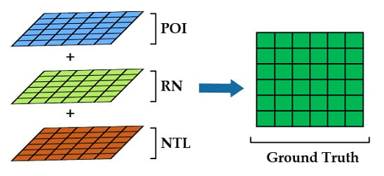
In this study, a general-purpose built-up area intelligent classification (BAIC) system that supports various types of data and classifiers was developed. Seven types of input data; namely, Point of Interest (POI), Road Network (RN), nighttime light (NTL), a combination of POI and RN data (POI_RN), a combination of POI and NTL data (POI_NTL), a combination of RN and NTL data (RN_NTL), and a combination of POI, RN, and NTL data (POI_RN_NTL), and five classifiers, namely, Logistic Regression (LR), Decision Tree (DT), Random Forests (RF), Gradient Boosted Decision Trees (GBDT), and AdaBoost, were tested in the BAIC. Training sample test samples are independent in the BAIC. Additionally, 30 m × 30 m pixel accuracy metrics were used to evaluate the performance of the BAIC. The research results can provide a reference for local urban planning and urban management departments. In the future, BAIC is expected to be used to provide large-scale maps of urban built-up areas.

2. Materials and Methods

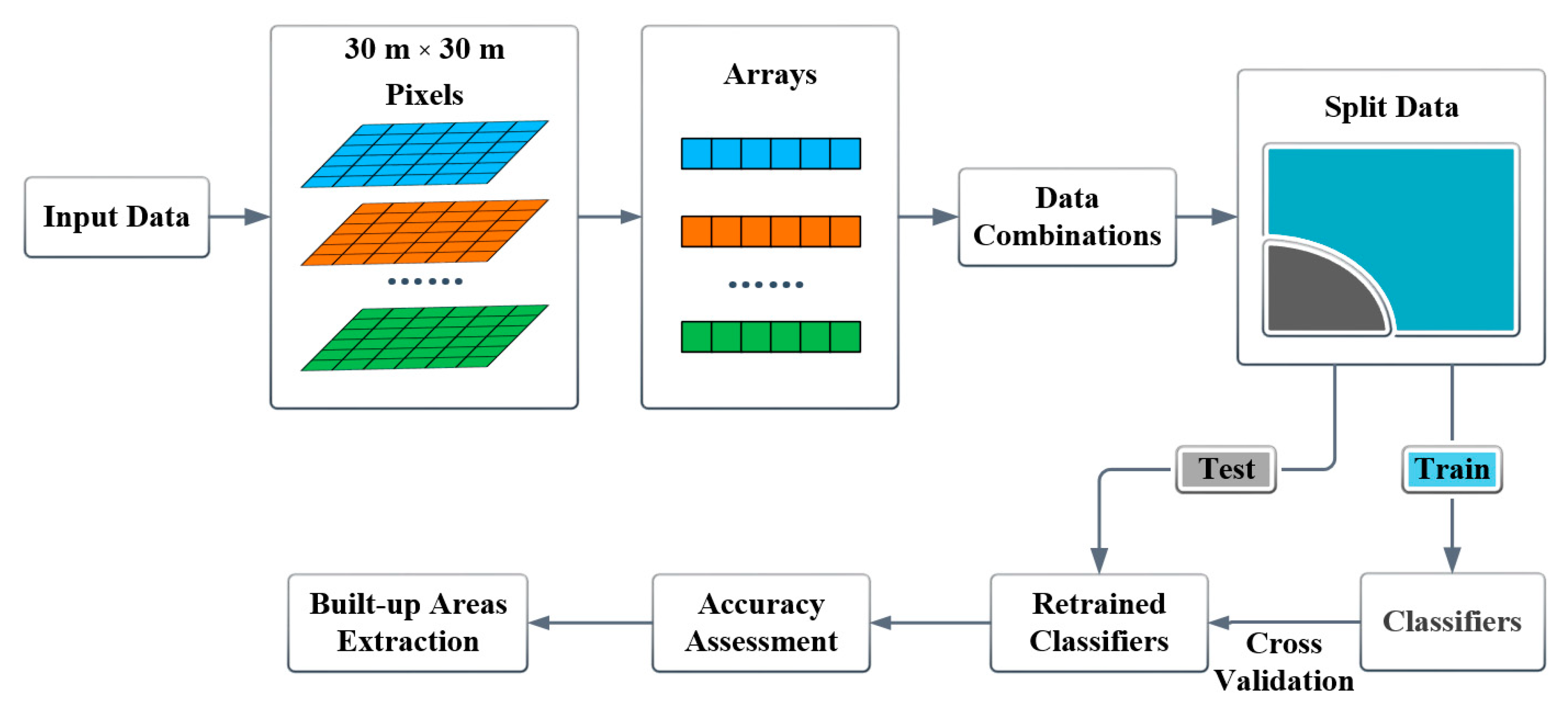
In this study, a BAIC system was developed using seven types of input data (i.e., POI, RN, NTL, POI_RN, POI_NTL, RN_NTL, and POI_RN_NTL) and five classifiers (i.e., LR, DT, RF, GBDT, and AdaBoost) to achieve intelligent extraction of urban built-up areas on a finer scale. The framework of the BAIC includes data preprocessing, image digitization (raster to arrays), data combinations, classifiers construction, accuracy assessment, and the extraction of built-up areas (Figure 1). The basic principle of BAIC is to translate the process of extracting urban built-up areas into the recognition of “1” (urban built-up areas) and “0” (non-built-up areas) of individuals 30 m × 30 m pixels. The initial classification results of BAIC were divided into four types (

Table 1. The four types of classification results.

Predicted Category
		1	0
Actual category	1	TP (True Positive)	FN (False Negative or Omission Error)
	0	FP (False Positive or Commission Error)	TN (True Negative)

TP: True Positive; that is, areas that were correctly classified as urban built-up areas. FP: False Positive; that is, areas that were incorrectly classified as urban built-up areas. FN: False Negative; that is, areas that were incorrectly classified as non-built-up areas. TN: True Negative; that is, areas that were correctly classified as non-built-up areas.

).

2.1. Study Area

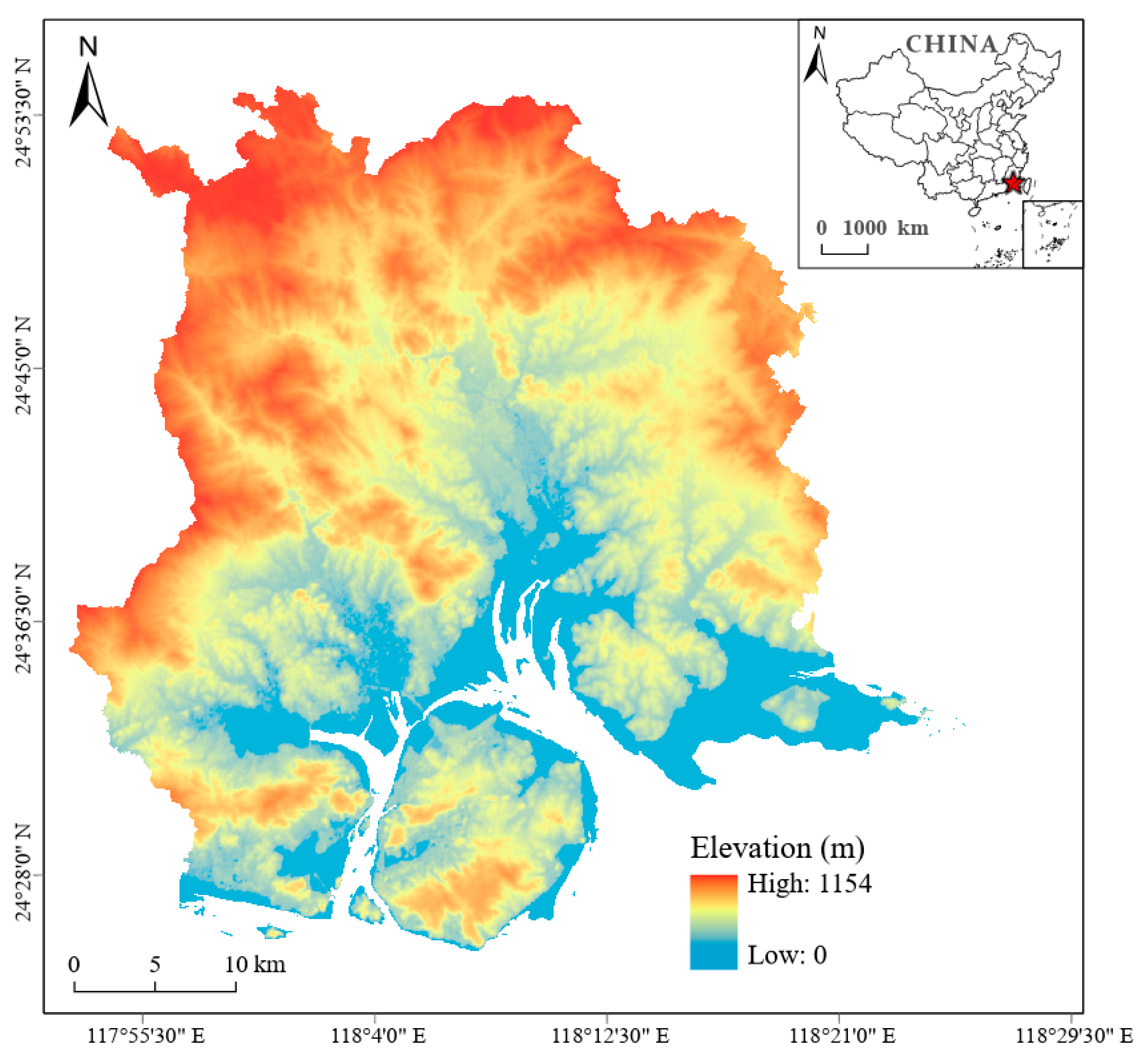
In this study, Xiamen City, Southeastern China, was selected as the research area. The city is located in southeastern Fujian Province and covers a land area of 1699 km² (Figure 2). Geographically, the city is composed of in-island areas and out-island areas. In this city, differences in the spatial distribution of natural resources, population, and economic growth have a significant influence on the structure of urban built-up areas. Therefore, Xiamen is a representative sample for research on extracting urban built-up areas. Additionally, there is spatial independence between in-island areas and out-island areas, which is favorable for splitting the training set and the test set.

2.2. Data Sources

2.2.1. Point-of-Interest (POI) Data

The POI data that were used in this study were obtained from the Gaode open platform web service in May 2019 (https://lbs.amap.com/api/webservice/summary) via a manually written Python program. A total of 62,501,795 POI records were obtained, covering the whole of China. A brief introduction to the data acquisition steps is given as follows: (1) divide the administrative boundary range of China into grids of an appropriate size and use each grid as the polygon of the query; and (2) construct bulk URLs for POI data for all primary categories through a polygon search mechanism and send an HTTP request to the Application Programming Interface (API) of Gaode’s search service. The API returns all data in JavaScript Object Notation (JSON) format inside the corresponding polygon, and the returned data are stored on a Structured Query Language (SQL) server.

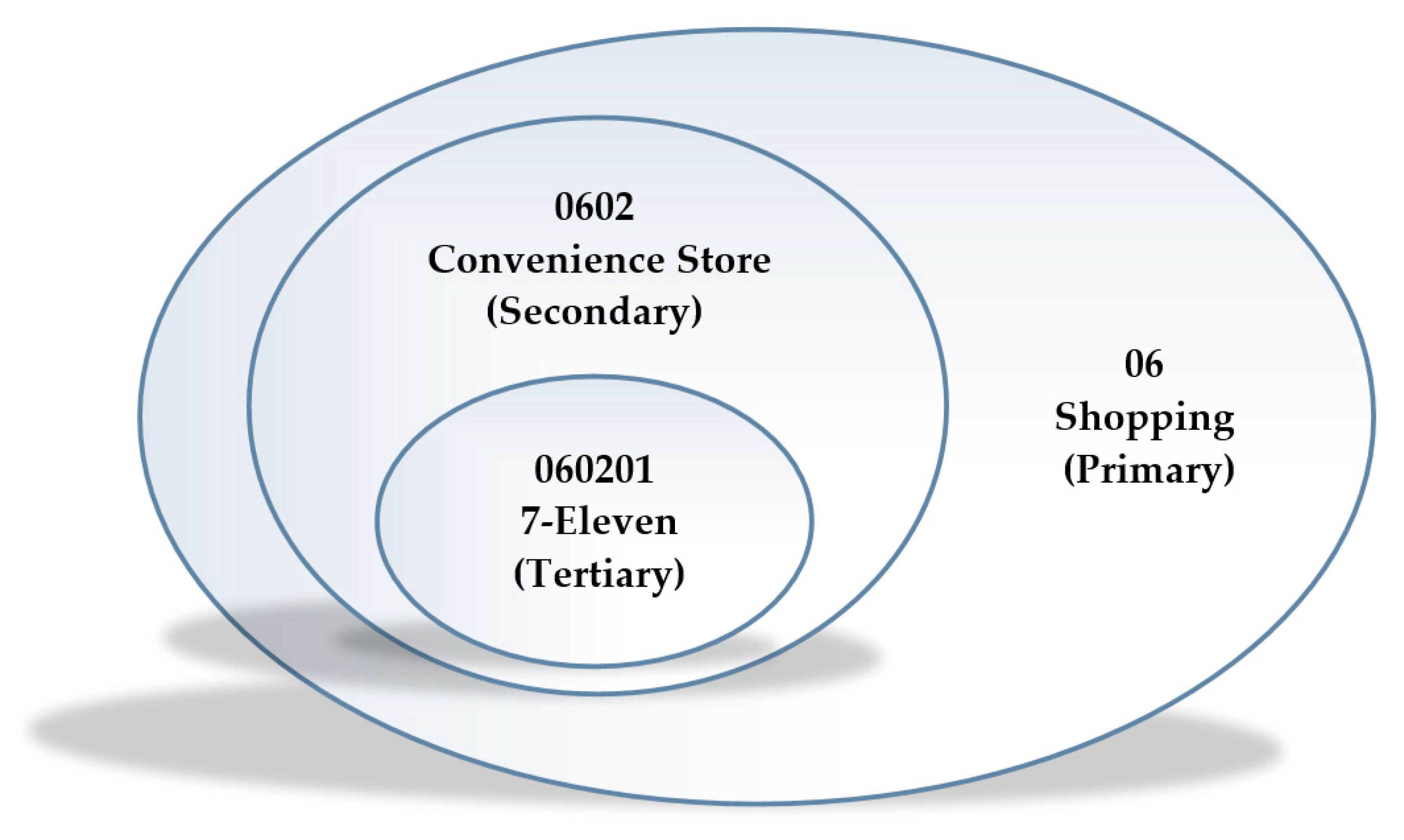
The Gaode map uses a three-level classification system for POI data (Figure 3). The category code for each POI datum consists of a six-digit decimal number; the first two digits of the category code represent the primary category; the middle two digits represent the secondary category, and the last two digits represent the tertiary category. The higher the classification of the category, the more detailed the classification of the data. The Gaode POI data have 23 primary categories, 264 secondary categories, and 869 tertiary categories. This study focuses on the primary category of Gaode POI data.

A typical Gaode POI record, such as the Bird’s Nest, is: {“id”: “B000A7GWO5”, “name”: “National Stadium”, “type”: “Sports and Recreation Service; Sports Venue; Comprehensive Gymnasium”, “typecode”: “ 080101”,”address”: “National Stadium South Road No. 1 Olympic Park”, “location”: “116.395777, 39.993427”, “citycode”: “010”, “cityname”: “Beijing”, “alias”: “Bird’s Nest “, …}. The “adname” field records the name of the county-level administrative region of the POI data. In the naming rules for the division of county-level administrative districts in China, the names of all administrative divisions include the following suffixes (in Chinese characters): “Zone”, “City”, “Domain”, “Flag”, “County”, “Island”, and “Administration”. Among these, the administrative division units whose names are suffixed with “district” and “city” are mostly distributed inside the urban built-up area. The administrative divisions whose names are suffixed with “domain”, “flag”, “county”, “island”, and “administration” are mostly distributed in the non-built-up areas. Based on the different suffixes of the “adname” field, a search for the “adname” field was conducted from more than 60 million POI data records for China. Then, the Transact SQL (T-SQL) statement in the SQL server was used to calculate the proportions of the various categories POI data that represent urban built-up areas and non-built-up areas (see result in Section 3.1).

Based on the proportional difference between urban built-up areas and non-built-up areas, six types of POI data (commercial house, enterprises, indoor facilities, pass facilities, public facilities, and transportation services) with a relatively high proportion in urban built-up areas were selected from the raw POI dataset (which contains 23 types of POI) and used to construct a combined POI dataset. A detailed description of these selected category tags and the non-selected category tags is shown in Appendix A.

2.2.2. RN and NTL

The RN data used in this study were obtained in February 2019 from the OpenStreetMap (OSM) website (https://www.openstreetmap.org/; data are available free of charge). The NTL data used in this study were monthly synthetic Visible Infrared Imaging Radiometer Suite (VIIRS) data acquired using the Day/Night Band (DNB) of the Suomi National Polar-Orbiting Partnership (S-NPP) satellite. The data can be downloaded directly from the website of the National Oceanic and Atmospheric Administration (NOAA) National Geophysical Data Center (NGDC) (https://ngdc.noaa.gov/eog/index.html).

2.3. Preprocessing

2.3.1. Kernel Density Estimation (KDE)

The KDE method is a non-parametric density estimation (NPDE) method that estimates the possible distribution of an indicator without assuming a density distribution or characteristic parameter. The method has been widely used in landscape ecology, engineering, medicine, and many other fields [27,28,29]. In the KDE method, it is assumed that a kernel function is characterized by adding the density of the $\mathrm{j}-\mathrm{th}$ sample point, and the kernel function is given by the following expression [30]:

$${\hat{\mathrm{f}}}_{\mathsf{\beta }}\left(\mathrm{X}\right)=(\mathrm{n}\cdot \mathsf{\beta }{)}^{-1}{\displaystyle \sum }_{\mathrm{j}=1}^{\mathrm{n}}\mathrm{K}\left(\left(\mathrm{X}-{\mathrm{X}}_{\mathrm{j}}\right)/\mathsf{\beta }\right))$$

(1)

where $K\left(x\right)$ is the symmetric probability density function, ${\mathrm{X}}_1,{\mathrm{X}}_2,\dots ,{\mathrm{X}}_{\mathrm{n}}$ is an observation sample selected from the n-dimensional population, and $\beta$ is the bandwidth.

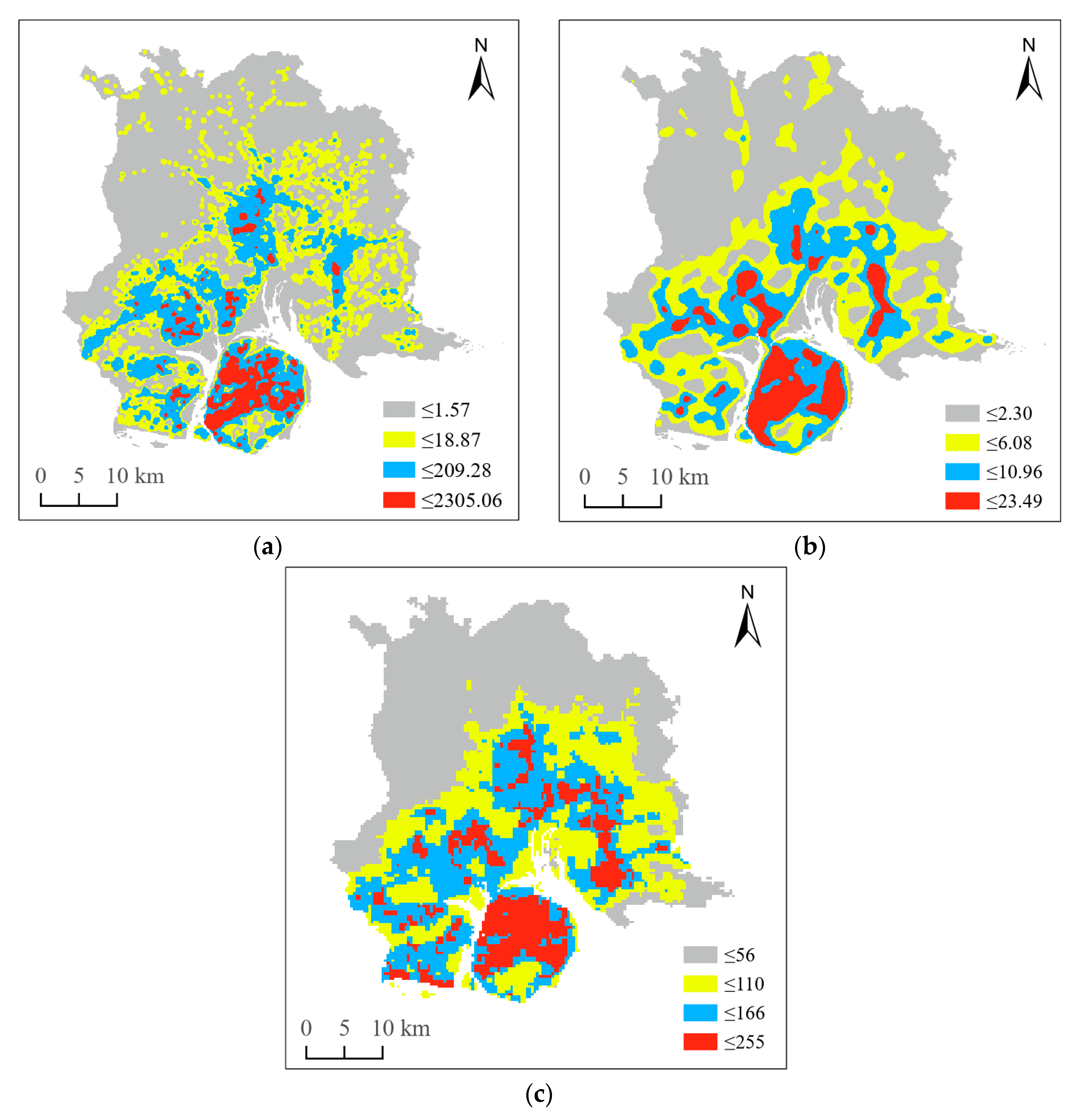
In order to transform POI and RN datasets into input format of the same scale suitable for the classifiers, KDE was used to convert the datasets into intensity maps (Figure 4a,b). A map of the NTL data was also generated (Figure 4c).

2.3.2. Rasterization and Combination

POI, RN, NTL, and ground truth were all transformed to the same coordinate system by projection transformation. All of the data were rasterized to 30 m × 30 m pixel data by resampling. Therefore, 30 m × 30 m pixel data are standard inputs in the BAIC. Seven data inputs, namely POI, RN, NTL, POI_RN (a combination of POI and RN data), POI_NTL (a combination of POI and NTL data), RN_NTL (a combination of RN and NTL data), and POI_RN_NTL (a combination of POI, RN, and NTL data) were generated from the three original inputs of POI, RN, and NTL.

2.4. Classification Algorithms

2.4.1. Logistic Regression

Logistic regression is a basic and common linear model used to solve classification problems [31]. It is also known as a log-linear classifier or logit regression. This model uses a logistic function to model the probabilities of the possible outcomes of the classification result.

2.4.2. Decision Tree (DT)

The DT method is a non-parametric supervised learning classification method that predicts the value of a target variable by learning specific decision rules from data features. The DT method has a simple structure that is easy for people to interpret, and it has therefore been widely used to solve classification problems in the field of remote sensing [32,33,34]. However, the DT method is unstable, since a small change in the train data may lead to a completely different tree structure, and individual DTs typically tend to cause overfitting and have low generalization ability. Using an ensemble of DTs such as RF or AdaBoost can mitigate this problem.

2.4.3. Ensemble Methods

Ensemble methods are usually placed into one of two categories: averaging methods or boosting methods. The basic principle of averaging methods is to independently build multiple estimators and then take the average of their predictions. The combined estimator usually achieves a reduced variance and has a better performance than the individual single-base estimator (e.g., a DT). Random Forests—an ensemble classification method composed of a large number of DTs which was first proposed by Breiman [35]—is a representative member of this category. In RF, each tree is built from a bootstrap sample from the training set. By taking the average of the predictions from diverse trees, RF can achieve a reduced variance and can remove some errors in individual decision trees.

By contrast, the driving principle of boosting methods is to built base estimators sequentially and to attempt to make the bias of the post-build estimator lower than that of the previously constructed estimator. Thus, a powerful ensemble is produced by combining several weak models. Gradient Boosted Decision Trees and AdaBoost are two representative members of this category. The former is a generalization of boosting to arbitrary differentiable loss functions; it is an effective and accurate off-the-shelf method that can be used for classification problems in a variety of areas including early warning of natural disasters and physical particle identification [36,37]. Meanwhile, AdaBoost, which was first introduced by Freund and Schapire in 1995 [38], is a very popular boosting method that has been widely used in classification problems [39,40].

Both averaging and boosting ensemble methods are insensitive to noise and outliers. In the proposed BAIC system, the three ensemble methods of RF, GBDT, and AdaBoost were combined.

2.5. Training and Validation

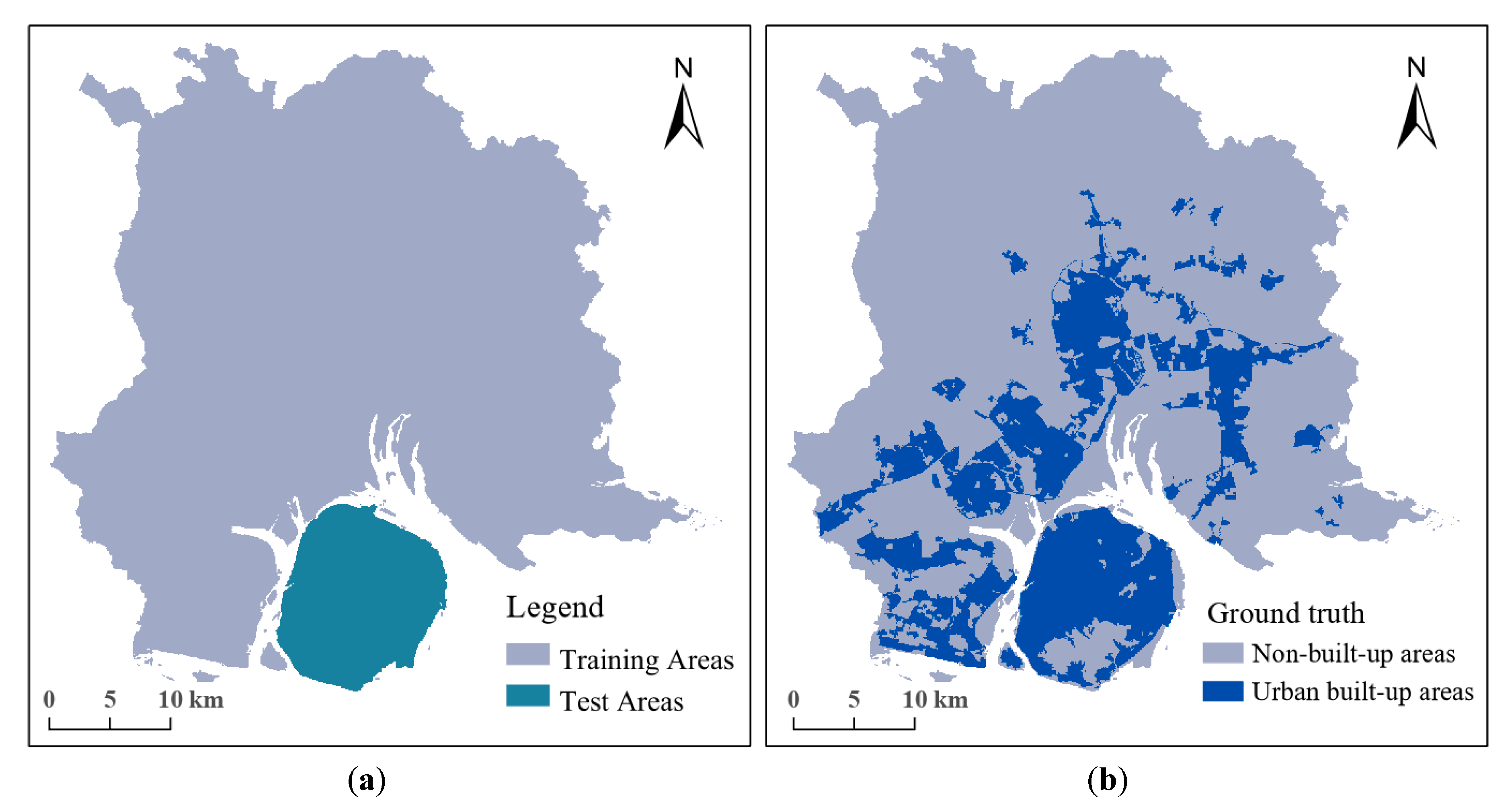
The in-island and out-island areas of Xiamen were selected as training and test areas, respectively (Figure 5a). In order to avoid overfitting, k-fold cross-validations were performed on the data in training areas to optimize the parameters of different classifiers or estimators in the training procedure. The principle of cross-validation is that the parameter with the largest average F₁-score was returned after k-times validation. Then, data in the test areas were used to measure the generalization performance of the classifiers in the validation procedure.

The ground truth which was used consisted of a collection of maps of the distribution of real urban built-up areas in Xiamen City provided by the Xiamen Municipal Natural Resources and Planning Bureau (Figure 5b). These maps were binarized, with a value of 1 being used for the urban built-up areas and a value of 0 being used for the non-built-up areas.

2.6. Accuracy Assessment

To assess the classification results for built-up areas, the F₁-score was calculated based on 30 m × 30 m grids in test areas. The F₁-score is a harmonic average of recall and precision; its value ranges from 0 to 1; the greater the value, the higher the accuracy. The F₁-score is given as:

$$F_1=\left(\frac{2}{{\mathrm{recall}}^{-1}+{\mathrm{precision}}^{-1}}\right)=2\cdot \frac{ \mathrm{precision} \cdot \mathrm{recall} }{ \mathrm{precision} + \mathrm{recall} }$$

(2)

where precision is also known as the user’s accuracy, and recall as the producer’s accuracy [41].

In this study, we considered the F₁-score to be a more important evaluation metric than the overall accuracy (OA) and Kappa statistic since the study area contains imbalanced land cover types [42,43]. We calculated OA in order to compare the results of this study with those of others that used only OA. Additionally, in order to determine the generalization ability of the BAIC, we plotted the receiver operating characteristic (ROC) curve and calculated the area under the ROC curve (AUC) [44]. The ROC curve was generated by plotting the True Positive Rate (TPR) against the False Positive Rate (FPR). TPR is a synonym for recall, and FPR is defined as follows:

$$FPR=\frac{FP}{FP+TN}$$

(3)

The ROC curve was used to evaluate the performance of the classification model at different classification thresholds. AUC is defined as the area enclosed by the coordinate axis under the ROC curve. AUC shows the average performance value of a classifier, which can be used to compare different classifiers. Additionally, AUC can be used to solve the problem of class imbalance. Both the ROC curve and AUC have been widely used in the evaluation of classification performance for classifiers [45,46,47].

3. Results

3.1. Distribution of POI within and outside of Urban Built-up Areas

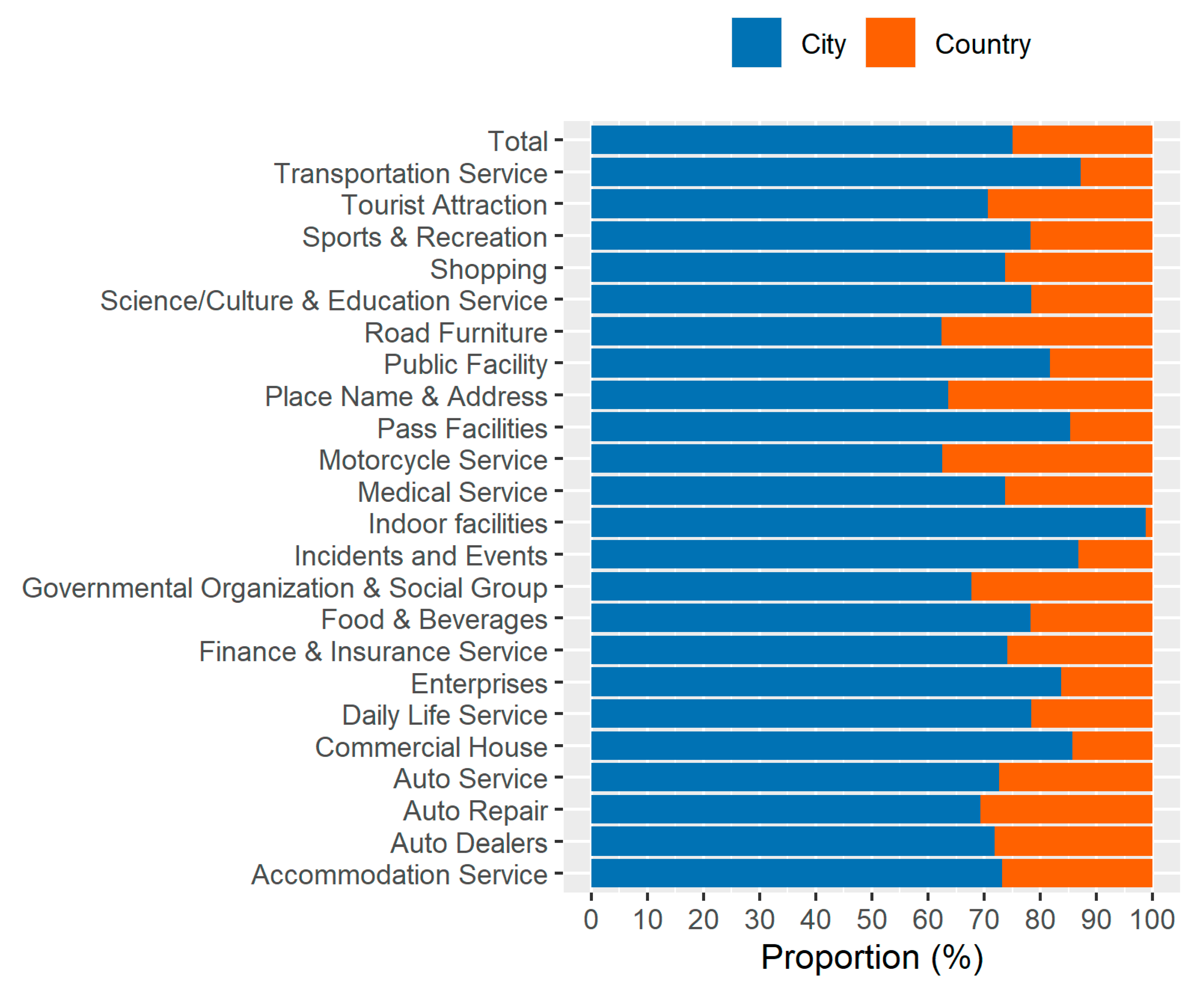
The results showed that there is a difference between the distributions of POI data in urban built-up areas and in non-built-up areas (Figure 6). POI data distributed in urban built-up areas accounted for about 75% of the total amount of POI data, almost three times the proportion of POI data distributed in non-built-up areas (25%).

Of the 23 separate categories of POI data, there were data from 18 categories in the urban built-up areas, accounting for more than 70% of the total number of categories, and data from five categories in the non-built-up areas, accounting for less than 30%.

3.2. Parameters Selection

The bandwidth of KDE has no significant effect on the results. At a gradient of 250–2500 m at 250 m intervals, the range of POI cross-validation scores differs among the five classifiers, however all of the scores are less than 0.07; similarly, the range of RN cross-validation scores differs among the five classifiers, however, all are less than 0.02. As a result, the bandwidths of POI and RN in KDE were selected as 250 m and 500 m, respectively.

Other key parameters obtained from the k-fold cross-validation results for the training set are as follows: the maximum depths of DT and RF were selected to be 2 and 4, respectively, and the learning rates of AdaBoost and GDBC were selected to be 1 and 0.1, respectively. The other parameters were set to the default values given in the scikit-learn Python library.

3.3. Extraction of Built-up Areas

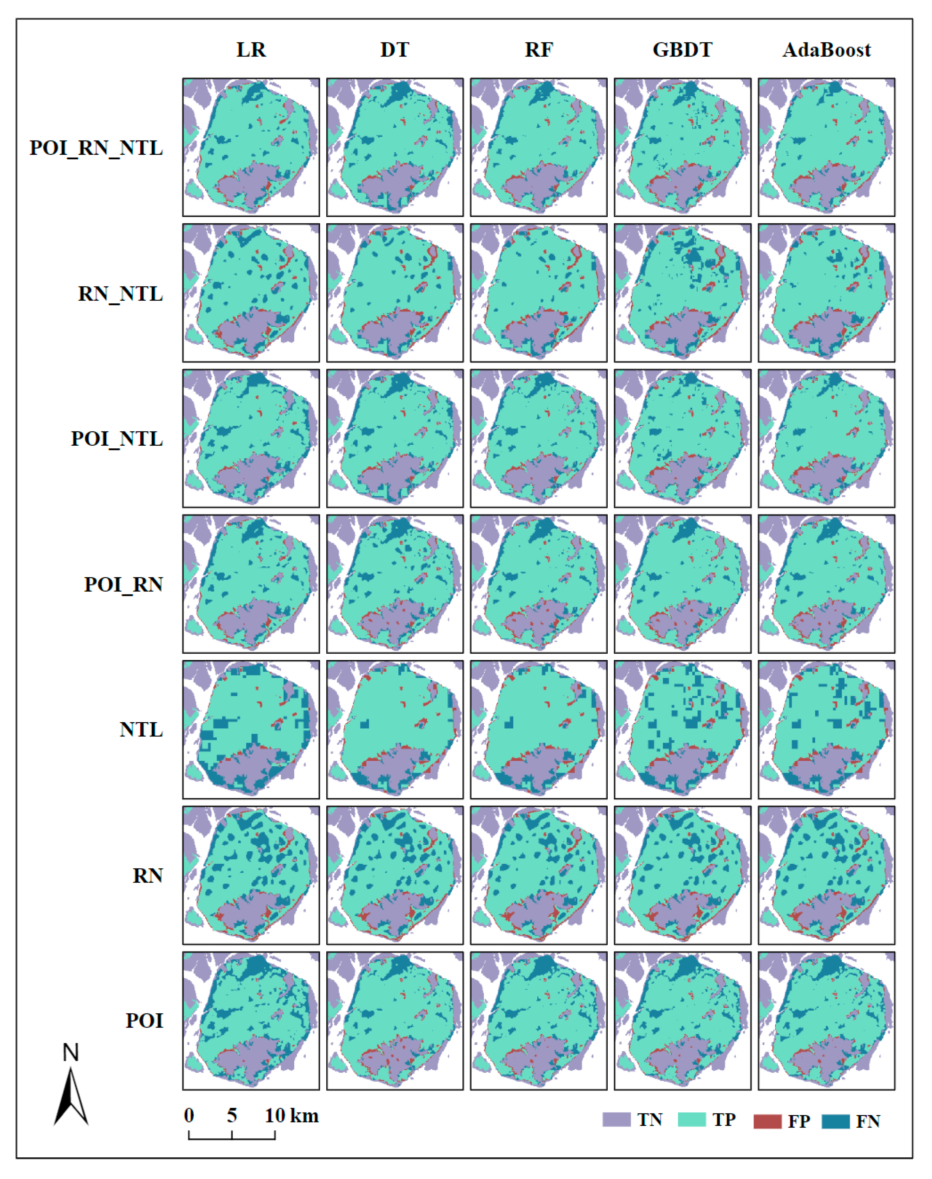
A total of 35 combination results were generated by BAIC using five classifiers and seven types of input data (Figure 7). Overall, there were more false negatives (FNs) than false positives (FPs) in the two situations where BAIC failed. Of all the data types, RN data clearly had the largest variance in spatial morphology because a large number of massive block urban built-up areas inside the test area were incorrectly identified as non-built-up areas. The combinations of two or three types of data had a lower spatial variance compared to single-input data. Of all the classifiers, the ensemble methods of RF, AdaBoost, and GBDT achieved a more stable classification performance than the traditional methods of LR and DT.

3.4. Accuracy Assessment

3.4.1. Overall Accuracy

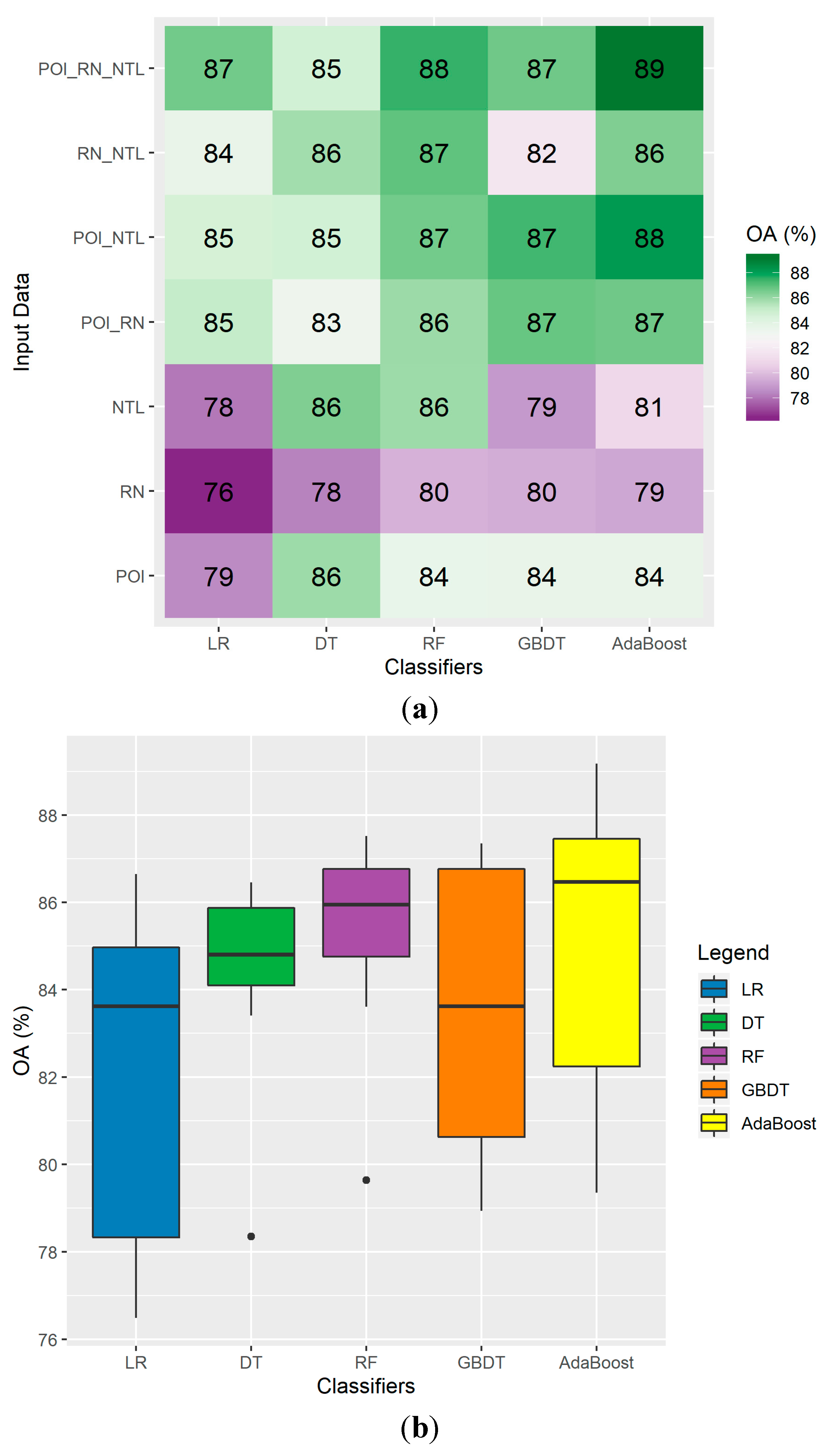
Among the 35 combinations between the five classifiers and seven types of input data, OA ranged from 76 to 89% (Figure 8). Overall, the largest OA was obtained using the POI_RN_NTL data and AdaBoost, while the smallest OA was obtained using RN data and LR. Most of the combinations of two or three types of data achieved a higher OA than single-input data.

3.4.2. F₁-score

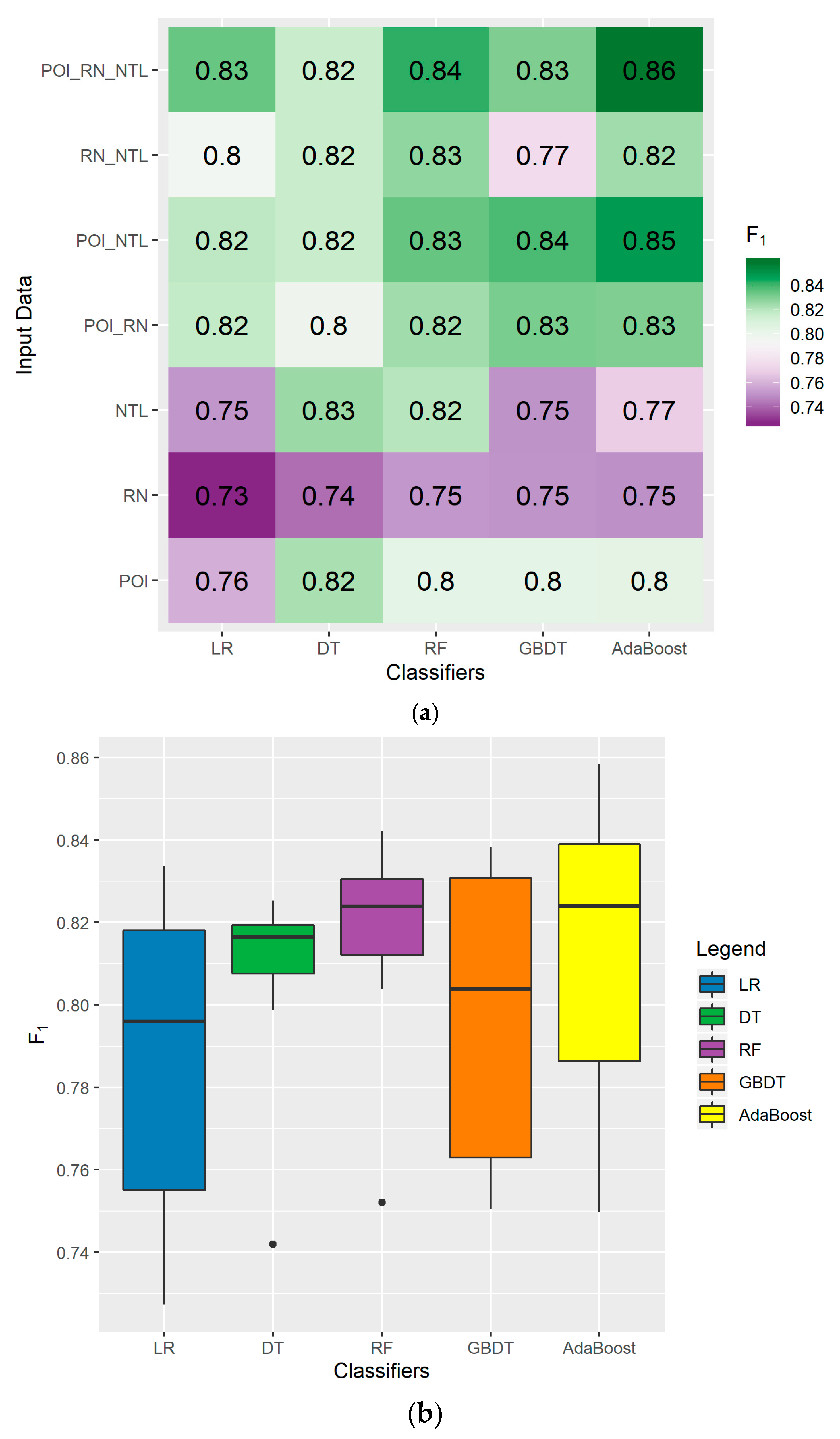
Among the 35 combinations between the five classifiers and seven types of input data, F₁ values ranged from 0.73 to 0.86 (Figure 9). Overall, the largest F₁ value was obtained using the POI_RN_NTL data and AdaBoost, while the smallest F₁ value was obtained using RN data and LR. Similar to the accuracy metric of OA, most of the combinations of two or three types of data achieved a higher F₁ value than single-input data.

3.4.3. AUC and ROC Curve

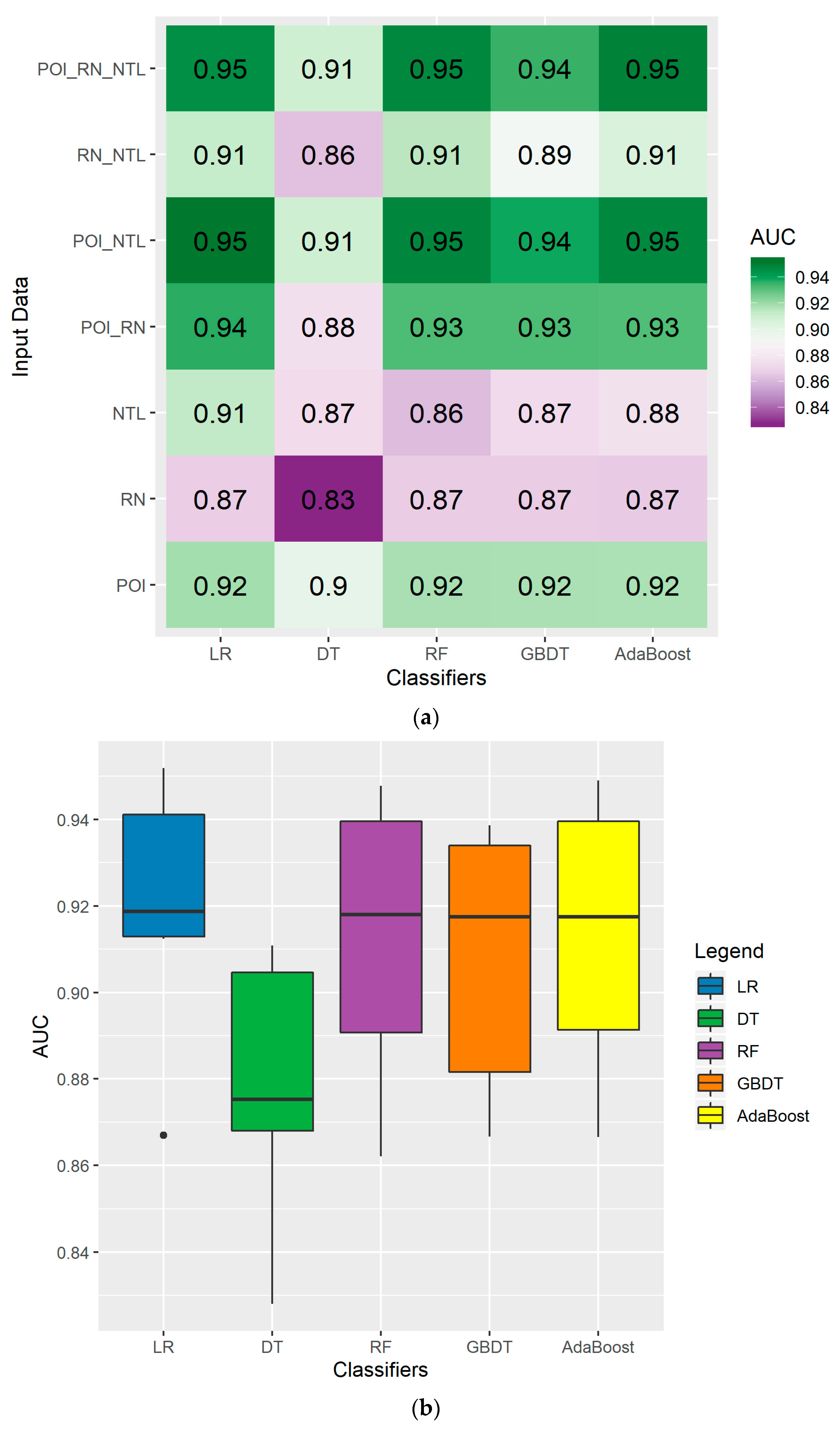
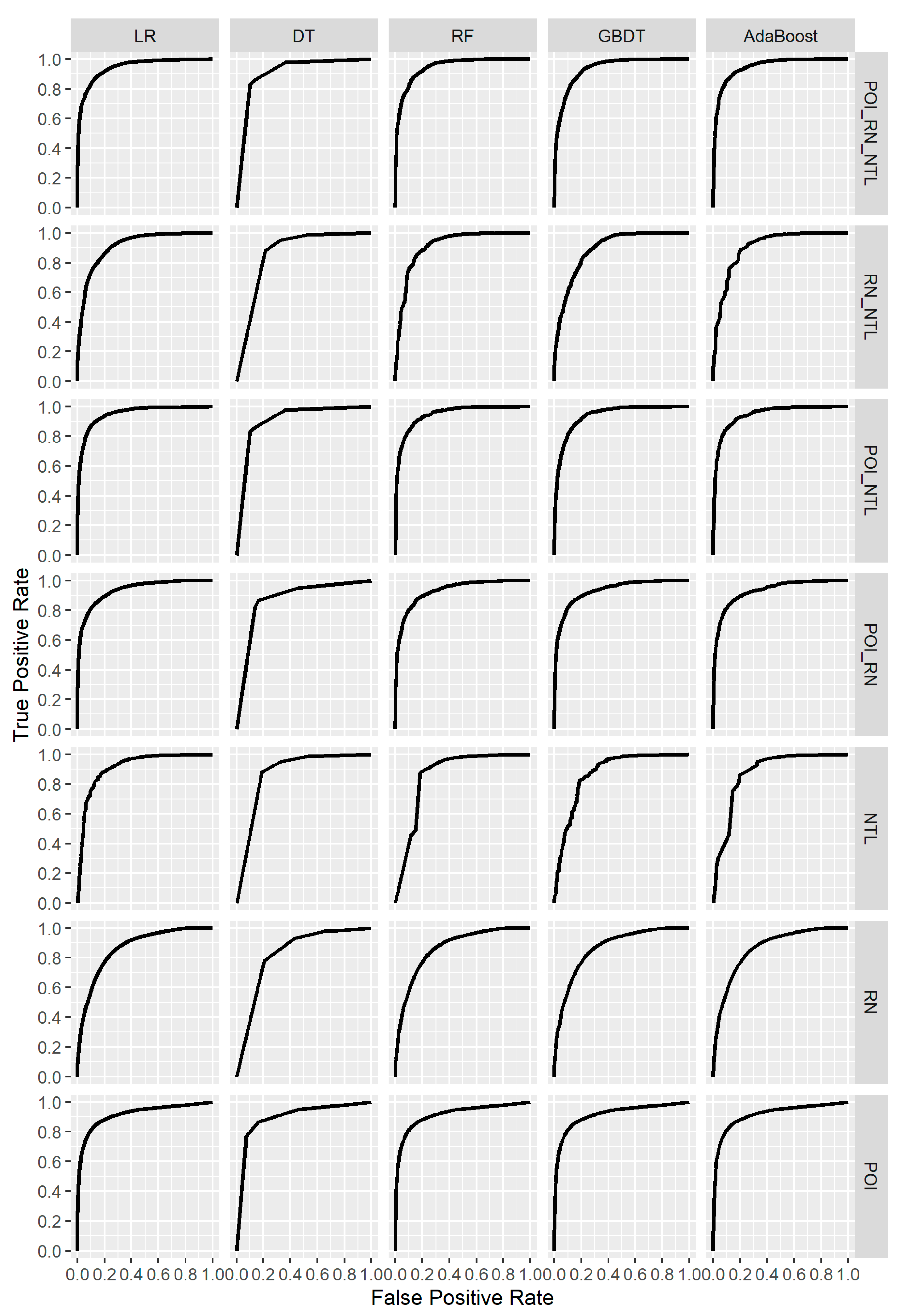
Among the 35 combinations between the five classifiers and seven types of input data, UC ranged from 0.83 to 0.95 (Figure 10). Overall, the largest AUC was obtained using POI_RN_NTL and POI_NTL data against AdaBoost, LR, and RF, while the smallest AUC was obtained using the RN data and DT. The ROC curves for the 35 combinations are shown in Figure 11.

4. Discussion

The BAIC has many distinct characteristics compared with previous classification systems. The first characteristic is the spatial independence of the test samples. Some studies that get final accuracy based on random sampling had mixed the training and test set in space, which will cause overfitting [19,24]. Similarly, other studies calculate accuracy by generating some random points and calculating the proportion of the number of correctly classified points in the same training area to the total number of points to obtain a final accuracy without testing in new areas, which may also cause overfitting [11,20,22]. The evaluation method of the BAIC is significantly different from that of similar studies. In BAIC, the use of k-fold cross-validation to optimize parameters in the training procedure does not mix the data between folds, therefore the test samples were spatially independent of the training samples. Furthermore, in the BAIC, the test areas used to calculate the 30 m × 30 m pixel-based accuracy were spatially independent of the training area. The spatial independence of test samples reduces the degree of overfitting and achieves a stronger generalization ability compared to validation procedures in similar studies. However, future study is needed to consider the spatial independence between test and training sets in the validation procedure. Additionally, for test sets, validation sample points should be collected from new test areas where no training sample points were collected from.

The second distinct characteristic of the BAIC is the final accuracy based on 30 m × 30 m grids is calculated in test areas independent of training areas. Compared to studies that calculate accuracy based on random sampling points [12,26], our pixel-based accuracy evaluation method is more objective and comprehensive, and additionally allows the comparison of the accuracy of different studies at the same scale.

The third distinct characteristic of the BAIC is that it allows the visualization of the spatial distribution of TPs, TNs, FPs, and FNs.

Furthermore, the fact that the BAIC uses three different types of open-source input data (POI, RN, and NTL) means that it is cheaper compared to classification methods that use commercial data. Moreover, the use of seven types of input data and five classifiers means that the BAIC is more robust than classifiers that only use one type of input data or classifier.

Grids of 30 m × 30 m were used in the data preprocessing. The reason that smaller grids were not used is that it would increase the running time of the BAIC, which would limit the application of the model on a large scale. Additionally, selecting a unit greater than 30 m would increase the resolution error (e.g., if 100 m was chosen, the error would be greater than or equal to 100 m).

In this study, the cross-validation of bandwidth for KDE showed that the classification results are insensitive to changes in bandwidth. Different cross-validation gradients will produce different optimal parameters. In the future, it would be meaningful to explore the impact of parameter optimization using different cross-validation gradients on the classification results.

5. Conclusions

In this study, a general-purpose built-up area intelligent classification (BAIC) system was developed supporting various types of data and classifiers. Additionally, a 30 m × 30 m pixel accuracy evaluation method that takes into account the spatial independence of test samples was proposed for the first time and used to evaluate the classification results. All of the steps in the BAIC were implemented using Python modules including Numpy, Pandas, matplotlib, and scikit-learn. Seven types of input data, namely, POI, RN, NTL, POI_RN, POI_NTL, RN_NTL, and POI_RN_NTL, and five classifiers, namely, LR, DT, RF, GBDC, and AdaBoost, were used in the proposed BAIC, and the results for each were compared.

The results show that, among the 35 combinations between the five classifiers and seven types of input data, the best classification performance was achieved using POI_RN_NTL as input data and AdaBoost as the classifier. Moreover, a lower variance was achieved using the combinations of two or three types of data. More robust classification results were obtained using ensemble methods of RF, GBDT, and AdaBoost compared to the traditional methods of LR and DT.

The advantages of using the BAIC include its multi-source input, more objective and comprehensive accuracy evaluation method, better generalization performance, lower cost, and strong robustness. Therefore, the proposed BAIC provides a new research avenue and an effective reference for the intelligent extraction of urban built-up areas using open-access RN, NTL, and POI data. This method can efficiently realize the automatic identification of urban built-up areas at a very low cost and can be easily applied to other urban areas in the world that have any kind of POI, RN, or NTL data coverage. The results of the present study are expected to provide timely and effective reference information for urban planning and urban management departments.

References

- Pendall, R.; Martin, J.; Fulton, W.B. Holding the Line: Urban Containment in the United States; Center on Urban and Metropolitan Policy, The Brookings Institution: Washington, DC, USA, 2002. [Google Scholar]
- Wentz, E.A.; Anderson, S.; Fragkias, M.; Netzband, M.; Mesev, V.; Myint, S.W.; Quattrochi, D.; Rahman, A.; Seto, K.C. Supporting Global Environmental Change Research: A Review of Trends and Knowledge Gaps in Urban Remote Sensing. Remote Sens. 2014, 6, 3879–3905. [Google Scholar] [CrossRef]
- Imhoff, M.; Lawrence, W.T.; Stutzer, D.C.; Elvidge, C.D. A technique for using composite DMSP/OLS “City Lights” satellite data to map urban area. Remote Sens. Environ. 1997, 61, 361–370. [Google Scholar] [CrossRef]
- Henderson, M.; Yeh, E.T.; Gong, P.; Elvidge, C.; Baugh, K. Validation of urban boundaries derived from global night-time satellite imagery. Int. J. Remote Sens. 2003, 24, 595–609. [Google Scholar] [CrossRef]
- Shi, K.; Huang, C.; Yu, B.; Yin, B.; Huang, Y.; Wu, J. Evaluation of NPP-VIIRS night-time light composite data for extracting built-up urban areas. Remote Sens. Lett. 2014, 5, 358–366. [Google Scholar] [CrossRef]
- Yu, B.; Tang, M.; Wu, Q.; Yang, C.; Deng, S.; Shi, K.; Peng, C.; Wu, J.; Chen, Z. Urban Built-Up Area Extraction from Log-Transformed NPP-VIIRS Nighttime Light Composite Data. IEEE Geosci. Remote Sens. Lett. 2018, 15, 1279–1283. [Google Scholar] [CrossRef]
- Gamba, P.; Lisini, G. Fast and Efficient Urban Extent Extraction Using ASAR Wide Swath Mode Data. IEEE J. Sel. Top. Appl. Earth Obs. Remote Sens. 2013, 6, 2184–2195. [Google Scholar] [CrossRef]
- Li, N.; Liu, F.; Chen, Z. A Texture Measure Defined Over Intuitionistic Fuzzy Set Theory for the Detection of Built-Up Areas in High-Resolution SAR Images. IEEE J. Sel. Top. Appl. Earth Obs. Remote Sens. 2014, 7, 4255–4265. [Google Scholar] [CrossRef]
- Xiang, D.; Tang, T.; Hu, C.; Fan, Q.; Su, Y. Built-up Area Extraction from PolSAR Imagery with Model-Based Decomposition and Polarimetric Coherence. Remote Sens. 2016, 8, 685. [Google Scholar] [CrossRef]
- Bhatti, S.S.; Tripathi, N.K. Built-up area extraction using Landsat 8 OLI imagery. GISci. Remote Sens. 2014, 51, 445–467. [Google Scholar] [CrossRef]
- Wang, L.; Zhu, J.; Xu, Y.; Wang, Z. Urban Built-Up Area Boundary Extraction and Spatial-Temporal Characteristics Based on Land Surface Temperature Retrieval. Remote Sens. 2018, 10, 473. [Google Scholar] [CrossRef]
- Zhou, Y.; Tu, M.; Wang, S.; Liu, W. A Novel Approach for Identifying Urban Built-Up Area Boundaries Using High-Resolution Remote-Sensing Data Based on the Scale Effect. ISPRS Int. J. Geo Inf. 2018, 7, 135. [Google Scholar] [CrossRef]
- Bogucki, R.; Cygan, M.; Khan, C.B.; Klimek, M.; Milczek, J.K.; Mucha, M. Applying deep learning to right whale photo identification. Conserv. Biol. 2019, 33, 676–684. [Google Scholar] [CrossRef] [PubMed]
- Cecconi, F.R.; Moretti, N.; Tagliabue, L. Application of artificial neutral network and geographic information system to evaluate retrofit potential in public school buildings. Renew. Sustain. Energy Rev. 2019, 110, 266–277. [Google Scholar] [CrossRef]
- Chaudhuri, T.; Soh, Y.C.; Li, H.; Xie, L. A feedforward neural network based indoor-climate control framework for thermal comfort and energy saving in buildings. Appl. Energy 2019, 248, 44–53. [Google Scholar] [CrossRef]
- Zhang, F.; Zhou, B.; Liu, L.; Liu, Y.; Fung, H.H.; Lin, H.; Ratti, C. Measuring human perceptions of a large-scale urban region using machine learning. Landsc. Urban Plan. 2018, 180, 148–160. [Google Scholar] [CrossRef]
- Zhang, H.; Li, J.; Wang, T.; Lin, H.; Zheng, Z.; Li, Y.; Lu, Y. A manifold learning approach to urban land cover classification with optical and radar data. Landsc. Urban Plan. 2018, 172, 11–24. [Google Scholar] [CrossRef]
- Wu, Q.; Lane, C.R.; Li, X.; Zhao, K.; Zhou, Y.; Clinton, N.; Devries, B.; Golden, H.E.; Lang, M.W. Integrating LiDAR data and multi-temporal aerial imagery to map wetland inundation dynamics using Google Earth Engine. Remote Sens. Environ. 2019, 228, 1–13. [Google Scholar] [CrossRef]
- Zhang, J.; Li, P.; Wang, J. Urban Built-Up Area Extraction from Landsat TM/ETM+ Images Using Spectral Information and Multivariate Texture. Remote Sens. 2014, 6, 7339–7359. [Google Scholar] [CrossRef]
- Ma, X.; Tong, X.; Liu, S.; Luo, X.; Xie, H.; Li, C. Optimized Sample Selection in SVM Classification by Combining with DMSP-OLS, Landsat NDVI and GlobeLand30 Products for Extracting Urban Built-Up Areas. Remote Sens. 2017, 9, 236. [Google Scholar] [CrossRef]
- Bramhe, V.S.; Ghosh, S.K.; Garg, P.K. Extraction of built-up areas from Landsat-8 OLI data based on spectral-textural information and feature selection using support vector machine method. Geocarto Int. 2019. [Google Scholar] [CrossRef]
- Forget, Y.; Linard, C.; Gilbert, M. Supervised Classification of Built-Up Areas in Sub-Saharan African Cities Using Landsat Imagery and OpenStreetMap. Remote Sens. 2018, 10, 1145. [Google Scholar] [CrossRef]
- Sun, Z.; Meng, Q.; Zhai, W. An Improved Boosting Learning Saliency Method for Built-Up Areas Extraction in Sentinel-2 Images. Remote Sens. 2018, 10, 1863. [Google Scholar] [CrossRef]
- Zhang, T.; Tang, H. A Comprehensive Evaluation of Approaches for Built-Up Area Extraction from Landsat OLI Images Using Massive Samples. Remote Sens. 2019, 11, 2. [Google Scholar] [CrossRef]
- Xu, T.; Coco, G.; Gao, J. Extraction of urban built-up areas from nighttime lights using artificial neural network. Geocarto Int. 2019. [Google Scholar] [CrossRef]
- Zhang, P.; Sun, Q.; Liu, M.; Li, J.; Sun, D. A Strategy of Rapid Extraction of Built-Up Area Using Multi-Seasonal Landsat-8 Thermal Infrared Band 10 Images. Remote Sens. 2017, 9, 1126. [Google Scholar] [CrossRef]
- Cai, X.; Wu, Z.; Cheng, J. Using kernel density estimation to assess the spatial pattern of road density and its impact on landscape fragmentation. Int. J. Geogr. Inf. Sci. 2013, 27, 222–230. [Google Scholar] [CrossRef]
- Ferracuti, F.; Giantomassi, A.; Iarlori, S.; Ippoliti, G.; Longhi, S. Electric motor defects diagnosis based on kernel density estimation and Kullback–Leibler divergence in quality control scenario. Eng. Appl. Artif. Intell. 2015, 44, 25–32. [Google Scholar] [CrossRef]
- Zhou, Z.; Si, G.; Zhang, Y.; Zheng, K. Robust clustering by identifying the veins of clusters based on kernel density estimation. Knowl. Based Syst. 2018, 159, 309–320. [Google Scholar] [CrossRef]
- Chiu, S.T. Bandwidth Selection for Kernel Density Estimation. Ann. Stat. 1991, 19, 1883–1905. [Google Scholar] [CrossRef]
- Hosmer, D.W., Jr.; Lemeshow, S.; Sturdivant, R.X. Applied Logistic Regression; John Wiley & Sons: Hoboken, NJ, USA, 2013. [Google Scholar]
- Friedl, M.; Brodley, C. Decision tree classification of land cover from remotely sensed data. Remote Sens. Environ. 1997, 61, 399–409. [Google Scholar] [CrossRef]
- Pal, M.; Mather, P.M. An assessment of the effectiveness of decision tree methods for land cover classification. Remote Sens. Environ. 2003, 86, 554–565. [Google Scholar] [CrossRef]
- Xu, M.; Watanachaturaporn, P.; Varshney, P.K.; Arora, M.K. Decision tree regression for soft classification of remote sensing data. Remote Sens. Environ. 2005, 97, 322–336. [Google Scholar] [CrossRef]
- Breiman, L. Random forests. Mach. Learn. 2001, 45, 5–32. [Google Scholar] [CrossRef]
- Lombardo, L.; Cama, M.; Conoscenti, C.; Maerker, M.; Rotigliano, E. Binary logistic regression versus stochastic gradient boosted decision trees in assessing landslide susceptibility for multiple-occurring landslide events: application to the 2009 storm event in Messina (Sicily, southern Italy). Nat. Hazards. 2015, 79, 1621–1648. [Google Scholar] [CrossRef]
- Roe, B.P.; Yang, H.J.; Zhu, J.; Liu, Y.; Stancu, I.; McGregor, G. Boosted decision trees as an alternative to artificial neural networks for particle identification. Nucl. Instrum. Methods Phys. Res. Sect. A Accel. Spectrometers Detect. Assoc. Equip. 2005, 543, 577–584. [Google Scholar] [CrossRef]
- Freund, Y.; E Schapire, R. A Decision-Theoretic Generalization of On-Line Learning and an Application to Boosting. J. Comput. Syst. Sci. 1997, 55, 119–139. [Google Scholar] [CrossRef]
- Hastie, T.; Rosset, S.; Zhu, J.; Zou, H. Multi-class adaboost. Stat. Its Interface 2009, 2, 349–360. [Google Scholar] [CrossRef]
- Rätsch, G.; Onoda, T.; Müller, K.R. Soft margins for AdaBoost. Mach. Learn. 2001, 42, 287–320. [Google Scholar] [CrossRef]
- Congalton, R.G.; Green, K. Assessing the Accuracy of Remotely Sensed Data: Principles and Practices, 3rd ed.; CRC Press: Boca Raton, FL, USA, 2019. [Google Scholar]
- Shao, G.; Wu, J. On the accuracy of landscape pattern analysis using remote sensing data. Landsc. Ecol. 2008, 23, 505–511. [Google Scholar] [CrossRef]
- Shao, G.; Tang, L.; Liao, J. Overselling overall map accuracy misinforms about research reliability. Landsc. Ecol. 2019, 34, 2487–2492. [Google Scholar] [CrossRef]
- Fawcett, T. An introduction to ROC analysis. Pattern Recognit. Lett. 2006, 27, 861–874. [Google Scholar] [CrossRef]
- Bradley, A.P. The use of the area under the ROC curve in the evaluation of machine learning algorithms. Pattern Recognit. 1997, 30, 1145–1159. [Google Scholar] [CrossRef]
- Hand, D.J. Measuring classifier performance: A coherent alternative to the area under the ROC curve. Mach. Learn. 2009, 77, 103–123. [Google Scholar] [CrossRef]
- Hajian-Tilaki, K. Receiver Operating Characteristic (ROC) Curve Analysis for Medical Diagnostic Test Evaluation. Casp. J. Intern. Med. 2013, 4, 627–635. [Google Scholar]
© 2019 by the authors. Licensee MDPI, Basel, Switzerland. This article is an open access article distributed under the terms and conditions of the Creative Commons Attribution (CC BY) license (http://creativecommons.org/licenses/by/4.0/).