Abstract
Temporal delays and spatial randomness between ground-based data and satellite overpass involve important deviations between the empirical model output and real data; these are factors poorly considered in the model calibration. The inorganic matter-generated turbidity in Lake Chapala (Mexico) was taken as a study case to expose the influence of such factors. Ground-based data from this study and historical records were used as references. We take advantage of the at-surface reflectance from Landsat-8, sun-glint corrections, a reduced NIR-band range, and null organic matter incidence in these wavelengths to diminish the physical phenomena-related radiometric artifacts; leaving the spatio-temporal relationships as the principal factor inducing the model uncertainty. Non-linear correlations were assessed to calibrate the best empirical model; none of them presented a strong relationship (<73%), including that based on hourly delays. This last model had the best predictability only for the summer-fall season, explaining 71% of the turbidity variation in 2016, and 59% in 2017, with RMSEs < 24%. The instantaneous turbidity maps depicted the hydrodynamic complexity of the lake, highlighting a strong component of spatial randomness associated with the temporal delays. Reasonably, robust empirical models will be developed if several dates and sampling-sites are synchronized with more satellite overpasses.
1. Introduction
The aquatic environments sustain great biodiversity and regulate a large number of physical, chemical and biological processes around them [1,2,3,4]; their preservation in the short term would be essential to face the strong impacts of the environmental transformation in large areas [5]. In the context of climate change, aquatic ecosystems such as shallow lakes acquire greater relevance due to their intrinsic fragility, but also their ability to regulate the regional climate; particularly, in the tropical strip which is considered as an extremely vulnerable region where the climate could be drier causing deep changes in the medium term [6].
The understanding of aquatic ecosystems demands more spatial and temporal resolution information; however, there are many difficulties to obtain analytical data from the water, especially when the body water has large dimensions. In this sense, satellite data has become an important source of information; remarkable advances in the development of satellite-based models have facilitated the water quality measurements with high frequency. This kind of model has been developed under two different methodologies: analytical and empirical approaches. The analytical models involve the measurement of Inherent Optical Properties (IOPs,) and the Apparent Optical Properties satellite reflectance measurement (AOPs), based on the Radiative Transfer Model (RTM) [7,8,9,10]. Unfortunately, the analytical method demands the use of infrastructure and equipment which is difficult to obtain in many cases.
Besides, the empirical models have been described as an alternative and easy method to recognizing the water quality status based on several optical properties, exploiting their computational simplicity; nevertheless, they have some disadvantages which should be taken into account in the final evaluation [11]. These models are technical and practically dependent on the AOPs retrieved from the Visible-Near Infrared spectrum (VIS-NIR); and the ground-based water measurements, together with the in-situ optical response; therefore, there are interference factors that reduce their certainty, inducing major complexity to the model construction. These complications have been partially overcome since the early studies in the 80s, using the optical response of several or specific sections of the electromagnetic spectrum [12,13,14]. Unfortunately, many of these models often have lacked critical image corrections to obtain a more accurate estimation [11]; other works have considered radiometric corrections to remove the optical effects and to retrieve a better water signal [15,16,17,18,19], although their methods entails more complex procedures for the satellite imagery management.
Another complication affecting the empirical model calibration is the strong dependence on the simultaneous (quasi-synchronous) satellite reflectance and ground-based data measurements (surface reflectance and water quality parameters) with the satellite overpass; these temporary delays could have implicit deviations derived from the water mass movement (spatial variations), decreasing the model certainty. Previous studies advise of such temporary variations, solving them with the data synchronization [13,20], others admit at least 1-day temporal delay [21,22,23,24,25]; however, the uncertainty level associated with the spatio-temporal relationship is not accentuated in the most cases. Few studies consider these factors in the model calibration; however, environmental and operational factors such as cloudy sky, low quantifications of water compounds (no representative events), or a reduced number of samples induce some model weakness [26,27].
The research related to shallow lakes has allowed an understanding of the interrelations among their natural components, and their connectivity to the basin system, establishing the water quality profile and its repercussions on the aquatic system. The discharge and displacement of sediments into shallow lakes have been considered as the most important factors contributing to its ecosystem balance; particularly, when the sediment resuspension is among the main regulatory process [5]. Two mechanisms determine this process depending of the lake zone: (1) Along the coast, the action of the waves mobilize the material deposited at the bottom of the water column; while (2) in the deeper areas, currents induced by seiche oscillations represent the most important factor that controls that sediment circulation through the water column [28,29,30]. Both mechanisms induce water turbidity, a physical property that affects other natural processes. The turbidity in water diminishes the transparency by the effect of light-scattering caused by organic or inorganic particulate material (e.g., phytoplankton and mineral sediments, respectively), producing great impacts on river and lake ecosystems [1,31]. Therefore, the turbidity has special attention on programs of monitoring carried out by international communities and institutions [32,33,34,35].
The present study aims to evaluate the effects of the temporal delays on the empirical model certainty for turbidity, considering the advantages of the Landsat-8 images, its NIR-bandwidth reduction, and the null organic matter incidence in these wavelengths. Daily and hourly delays were assessed in the calibration process to estimate the output model prediction-related error. The models were calibrated with the ground-data taken from this study; while the official measurements of the National Water Council (NWC) help to evaluate the model response. These results were compared with the ground-based measurements modeled through geostatistical analysis; highlighting the instantaneous horizontal turbidity configuration, and the high spatial resolution of the satellite-based empirical model. Lake Chapala was used as a study case because of its ecological importance to the west of Mexico. The results obtained in this study emphasize the importance of the data source synchronization to obtain better model predictions.
2. Methods
2.1. Lake Chapala
Lake Chapala is the largest inland lake in Mexico, covering an area of ~1100 km2, with a length of 75 km and a width of 5.5 km approximately in the western sector and up to 20 km to the east (Figure 1). The lake reaches its maximum capacity at the 1523.8 masl (relative level of 97.8 m established by the Water Council of the State of Jalisco), it has an average and maximum depth of 4.5 and ~8 meters, respectively; and a maximum volume of ~7900 Mm3 [36]. The lake was classified as one of the largest and shallowest tropical-lakes in the world [37,38]. This lake has a hydrodynamic complexity that favors the horizontal scrolling of long internal flows, with currents reaching average speeds between 2 and 30 cm s−1 caused by winds of 5 to 8 m s−1 [39,40,41], which are capable to move water masses along some tens of meters or even more than 1 km per hour. The lake hydrodynamic involves a strong component of spatial randomness associated with the temporal delays between satellite overpass and in-situ information, which would affect the development of empirical models.
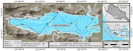
Figure 1.
Map of Lake Chapala. Abbreviations: National Water Council (NWC); Shuttle Radar Topography Mission (SRTM); National Aeronautics and Space Administration (NASA); and The Land Processes Distributed Active Archive Center (LPDAAC).
The Lerma river is the main source of sediments and turbidity of the Lake Chapala. The river belongs to one of the largest basins in the country, which has a surface of 47,116 km2 and a mean annual surface runoff of 4742 Hm3 [42]. The Lerma river carries a great amount of solids generated by erosive processes, mainly caused by poor management of soil resources [43,44]. The river also transports contaminants from upstream towns to the lake due to the agricultural, livestock and industrial activities; many of these effluents are not treated and constitute a potential threat to the ecosystem of the lake and further downstream [45,46]. La Pasión Creek is another important source of sediment, which causes turbidity in the lake [47]. In its river catchment, extensive deforestation contributes to large-scale soil erosion [48], producing large amounts of sediment to enter the lake.
Previous studies have characterized the clay turbid waters along the Lake Chapala, where the high Total Suspended Solids (TSS) concentrations range between 13 and 420 mg L−1 [37,47,49]. It is a medium where the phytoplankton typically are light-limited, with low to moderate Chlorophyll a (Chl a) concentrations, which commonly range in the order of 0.9 to 33.5 µg L−1 (11 µg L−1 on average) [36,49,50,51]. Given these properties and taking the lake’s classification based on the biological activity described by Chapman [1], Lake Chapala could be classified with a low to moderate eutrophic degree, usually related to the presence of nutrients such as nitrates and phosphates.
2.2. Ground-Based Data
2.2.1. Information Sources
Two different data sources were used in this study. The ground data taken in this study helps to calibrate the model approach; while, the dataset of NWC was used to evaluate the model estimations. The council manages the national water monitoring network in Mexico, their Laboratory Consortium measures a set of water quality parameters in 34 sites inside the lake (Table 1), having the Chl a, TSS, and turbidity among the parameters of interest for this study. The NWC follows national and international standards to the parameter determinations; in this sense, the Chl a measurement derived from the extraction method 10200-H described in the American Public Health Association, APHA [52]; the TSS are determinate under the Mexican standard NMX-AA-034-SCFI-2015 procedures; while, the turbidity determination follows the nephelometry method referred in the NMX-AA-038-SCFI-2001.

Table 1.
Sampling sites in Lake Chapala.
These parameters are measured at least two times in the year and the average values are published since 2006 in the water quality website (http://sina.conagua.gob.mx/sina/); however, the most complete and continuous time series have been identified only in the recent period (2012–2018). This data source exploration together with previous studies [36,38,47,51] helped to understand the most common spatial distribution of the water turbidity in Lake Chapala.
Besides in this study, two sampling campaigns were conducted to obtain information from Lake Chapala. Two brigades simultaneously covered two different routes in Lake Chapala to measure the properties of the water (Figure 1). The first sampling was carried out during the wet season of 2016 (September 6); while the second was held in the dry-warm season of 2017 (April 24). The field trip in both campaigns had an approximate duration of 7 hours (between 10 a.m. to 5 p.m., local time). The sampling was systematized obtaining a homogeneous spatial distribution of the sites; all the fifteen sampling sites were close to another established by the NWC (Table 1), therefore both data sources similarly describe the spatial variations of the water parameters.
In Lake Chapala, the water transparency is attenuated at 30 to 50 cm depth [50], although it could occur at 80 cm depth in some areas [51]. Since the water transparency decreases due to the matter contents, the sampling depth becomes an important subject in the remote sensing of the water. In this sense, all the samples were taken at 1 m depth to retrieve the greatest possible amount of energy reflected coming from the upper level of the water column. The water samples were stored in 1-liter amber bottles previously upgraded under laboratory conditions; during its translation, the samples were isolated at a temperature <4 °C to preserve the in-situ properties of the water. The water samples were measured by triplicate, and the mean value was taken for each parameter in all the sites.
The TSS was determined according to the standardized method for the water examination described in section 2540-D (Physical and aggregate properties) of the APHA [52]. The water samples were filtered by a 1.2 μm glass-fiber (Whatman GF/C, diameter: 21 mm) previously weighted and dried, obtaining a residual mass of 200 mg; the residual matter was dried at ~103 to 105 °C during 1 h with a lab oven (Quincy Lab. Inc, 40-GC model). The turbidity was determined using an optical method and calibrated in terms of the Nephelometric Turbidity Unit (NTU); a scanner (Hach 2100AN-SI) measured the light dispersion in the interval of 860 ± 10 nm taken into account the standard ISO 7027-1:2016. This study assumes low Chl a concentrations only based on historical data.
The method used in this study for the TSS is the same as that used for the NWC, therefore, minimal differences were assumed between datasets. On the other hand, the method used for the turbidity in both cases follows the same optical technique, although the range of measurement (400–600 nm) employed by the NWC implicates the spectral signal of some organic compounds.
2.2.2. Statistical Tests
The parameters of TSS, Chl a, and turbidity were subjected to a statistical evaluation to know their distribution type. This step helps to conduct appropriated statistical tests to determine the primary turbidity source in Lake Chapala. The water parameters were analyzed using the Shapiro-Wilks test, this is one of the most strict tests to probe the normal distribution [53,54]. It was found that all parameters lacked normal distribution; therefore, non-parametric tests were used to measure the correlation degree among variables (Spearman’s ranks, r2), as well as the heterogeneity among dataset (Mann-Whitney U, MWU). All the statistical tests were carried out with a significance of <0.05 referred by the p-value.
2.2.3. Geostatistical Evaluation
These datasets also were subjected to a geostatistical analysis following Johnston et al. [55]. The ordinary kriging was used as an interpolator for the map prediction given that this offered a better approach; this model takes advantage of the spatial autocorrelations to estimate the effects of local and regional behavior of the variable [56]. The map predictions were based on an empirical semi-variogram, a linear estimator, and the unknown weights calculations. This unbiased predictor also lets us estimate the probability and accuracy of the water parameters in the lake. Specifically, the quality of all the prediction models was evaluated using two statistical parameters: the root means square standard error (RMSE) help us to compare and choose the best fit model; while, the mean error (ME) evaluates the accuracy of the model prediction. The probability to overcome the average values of every statistical variable was estimated for the water parameters; while, the standard error (SE) was used to estimates the spatial prediction uncertainty.
2.3. Satellite Imagery
2.3.1. Turbidity and NIR Reflectance Relationships
The turbidity is mainly caused by particles of solid matter suspended in water; however, some dissolved light-absorbing substances affect its quantification in the region of the visible spectrum (VIS) [57,58]. Therefore, high-accuracy optical methods such the standard ISO 7027-1:2016 have been implemented to quantify the analytical turbidity approach [59]; the method suggests the turbidity quantification at the NIR wavelengths (860 ± 10 nm) to avoid the interference effects derived from dissolved compounds in the water, recovering a sharper turbidity response.
On the other hand, the Landsat program developed by the National Aeronautics and Space Administration (NASA) had assessed the status and evolution of natural resources. It has been a data source for the remote sensing of the water and its constituents, including turbidity. The Landsat-8 satellite generates images of moderate spatial resolution (30 m), this platform has had several changes that make it better than the previous versions; one of the most important for the turbidity analysis is the bandwidth reduction in the NIR, from 772–898 nm (TM and ETM+) to 851-879 nm [60]. This change implicates great advantages in the remote sensing of turbidity due to the adjustment to the standard measuring range established by the ISO 7027-1:2016.
2.3.2. Surface Reflectance
The USGS uses the Landsat-8 Surface Reflectance Code (LaSRC) to generate Top of Atmosphere (TOA) reflectance and Brightness Temperature (BT) images based on the calibration parameters of the images and mathematical models [60]. The code proposed by Vermote et al. [61] also removes the atmospheric and topographic effects based on the auxiliary data taken from MODIS and GTOPO5 to improve the surface reflectance images (Collection 1 Level 2: C1L2, on-demand products); Additionally, the LaSRC also reduces the bidirectional effect associated to the geometric relationships between the Sun and sensor angles [62,63,64]. These images offer accurate measurements of the surface reflectance held above the Earth’s surface, increasing the consistency and comparability between images taken at different times [65]; therefore, their quality is much better than the conventional Landsat-8 level-1 images. Having this advantages, fourteen (C1L2) Landsat-8 multispectral images available to the Lake Chapala (Table 2) were used to detect the water-leaving irradiance reflectance between March 2016 and September 2017 (Collection 1 Level 2, on-demand products from earthexplorer.usgs.gov); the standardization of these products help us to carry out a temporal analysis with higher certainty.
Table 2.
List of Landsat-8 images.
2.3.3. Spectral Improvement
Inland surface-waters absorb high proportions of solar energy, reflecting negligible quantities to space; the energy reflected typically represents less than 10% of the total incoming energy [66]. The low-reflectance of the water involves important challenges to recover the optical response of its constituents, even when the image contains the Earth’s surface reflectance corrected by atmospheric and topographic effects. Therefore, additional to the implicit corrections of the LaSRC products, two complementary processes were used to improve the remote sensing of the water.
The first post-processing was focused on the delineation and confirmation of the water surface, removing the clouds and cloud-shadows interferences. It is a simple pixel subtraction based on the aerosol and pixel-quality assessment bands generated by the LaSRC; which identify the surfaces where the physical and chemical aerosols-properties could produce strong perturbations on the VIS-NIR surface reflectance [61]. The second post-processing was related to the sun-glint effect correction, corresponding to the specular reflection from the upper side of the air-water interface to the satellite detector; this effect is considered as one of the greatest factors affecting the quality and accuracy of the water optical response after the atmospheric interference [67]. The sun-glint effect on the Landsat-8 images was attenuated with the use of a statistical method [17]. This method removes the noise manifested at the VIS-wavelengths supporting on the NIR band. They assumed that water has a high energy absorption capacity in the NIR, which produces a negligible light dispersion coming from different levels of the water column or the signal from the bottom.
In this study, the NIR band used by Lyzenga et al. [17] was replaced by the SWIR-2 band (2107–2294 nm). It has proved that the NIR-reflectance is not the best band to carry out the sun-glint effect correction, given its capacity for retrieving the optical response of suspended matter in turbid waters [67,68,69]; where a noise signal caused by moderate concentrations could produce major uncertainties or the light-saturation effect in the NIR-reflectance during the correction process [15]. Instead, the SWIR reflectance has been proposed as a better way to reduce the backscattering light effect [70]; where the extinction coefficient of the water (clear or turbid) is the highest and its refraction index is lower than other wavelength regions within the solar spectrum of ~400–2500 nm [71]. Previous studies have used the spectral response of the water in the ranges of 1240 to 2130 to improve the radiometric analysis upon coastal zones or rivers, allowing good approaches [72,73]. Given such advances, the Lyzenga’s method based on the Landsat-8 SWIR-2 band has also improved the sun-glint correction in the NIR band, which was used to retrieve the water turbidity.
3. Results
3.1. TSS-Turbidity Correlations
3.1.1. Factor Assessment
A multiple-variable analysis was carried out to identify the parameter (TSS or Chl a) which drives the variability of the water turbidity. A set of 218 paired samples from 34 NWC-sites exposed that the turbidity-TSS covariate better than the turbidity-Chl a ones. Both, TSS and Chl a had a significant relationship with the turbidity (p = 0.0 in both cases); however, the Spearman’s coefficient indicated that the TSS had a moderate correlation with the turbidity (r2 = 0.49), better than the Chl a (r2 = 0.31) (Figure 2). Based on these results, the TSS was recognized as the main factor controlling the water turbidity in Lake Chapala.
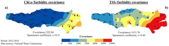
Figure 2.
Geostatistical analysis in Lake Chapala, (a) covariance between Chl a and turbidity, (b) covariance between TSS and turbidity.
Consequently, a sharp geostatistical analysis was focused on the TSS and turbidity to evaluate their spatial behavior, considering their mean and maximum values. The quality of the TSS and turbidity spatial predictions were sustained on the best fit model forecaster, ensuring their high quality through RMSSE close to the reference value (1.0) (Figure 3 and Figure 4). The accuracy of the obtained models was very close to the reference value (ME = 0.0), except for the maximum TSS concentrations, which showed a high value (0.402). While, the model prediction uncertainty was the lowest among the mean values of both water parameters (SE < 8%) in almost all the lake; opposite to the maximum values with uncertainties higher than 30% up to 100% for TSS, and 10 to 30% for turbidity.

Figure 3.
Geostatistical analysis of the total suspended solids (TSS) in Lake Chapala. Concerning to the mean TSS concentrations: (a) Prediction map, (b) Probability to overcome the average values, and (c) Spatial distribution of the standard error. Concerning to the maximum TSS concentrations: (d) Prediction map, (e) Probability to overcome the average values, and (f) Spatial distribution of the standard error.
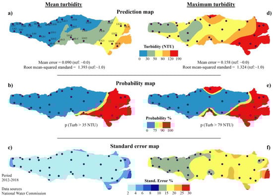
Figure 4.
Geostatistical analysis of the turbidity in Lake Chapala. Concerning to the mean turbidity quantifications: (a) Prediction map, (b) Probability to overcome the average values, and (c) Spatial distribution of the standard error. Concerning to the turbidity quantifications: (d) Prediction map, (e) Probability to overcome the average values, and (f) Spatial distribution of the standard error.
3.1.2. Geostatistical Analysis
The basic statistics of the 34 sites reveal that the annual mean TSS concentrations during the period 2012–2018 were in the range of 11 to 262 mg L−1 (average: 48 mg L−1); while the annual maximum values were between 11 and 475 mg L−1 (average: 140 mg L−1). The concentrations were in the same order to those reported by the official sources to the period 1974–1997 when the mean values ranged between 23 and 144 mg L−1 (average: 41 mg L−1) and the maximum reaching up to 402 mg L−1 [47]. The analysis indicates the mean TSS concentrations increase to the eastern end of the lake; in these areas, the probability to overcome the annual average values indicates that it would be higher than 90% in the coming short-term (Figure 3a–c). The maximum TSS values have been higher along the eastern shoreline and the center of the lake, where the probability to overcome the annual average values is higher than 90%. The general spatial distribution indicates that the punctual concentrations have remained higher in the eastern side, at least during the recent years. Notwithstanding, the natural high-statistical scattering of the maximum TSS values produced spatial randomness, inducing a biased model-prediction with a ME much higher than the expected value (~0.0). Such deviations had affected the model certainty manifested by high SE-values along the lake (SE > 30%), which increases as we move away from the sampling site (Figure 3d–f).
On the other hand, the annual mean turbidity quantifications were in the range of 11 to 147 NTU (average: 35 NTU), and the maximums between 32 and 190 NTU (average: 79 NTU); all in accordance with previous studies [50,74]. The geostatistics reveals that the mean and maximum values of turbidity have a gradient increasing to the eastern side (similar to the mean TSS). The maximum turbidity has been higher in some places along the south and northern shoreline, where the probability to overcome the average value is higher than the 90%; unfortunately, the SE has been of the order of 15–25%, higher than the expected value; reducing the model certainty at the eastern side of the lake (Figure 4).
3.2. Analysis of the Ground-Based Measurements
The NWC-dataset confirms the TSS concentrations represent the primary turbidity source in Lake Chapala in recent years. Therefore, the TSS and turbidity ground-based data obtained in this study were analyzed to establishing direct relationships with the water-leaving irradiance reflectance from the lake, necessary to the empirical model development. Then, a previous statistical assessment was carried out to identify seasonal or spatial variations, this is to ensure major certainty for the model calibration.
Spatial and Seasonal Behavior
The MWU-test was used to compare datasets between seasons and zones of the lake. The TSS concentrations observed in both season range between 135 and 342 mg L−1. The MWU-test showed no significant differences (p = 0.130) between the median values of the seasons (spring and summer-fall); however, it was found that the TSS were highest on the eastern side considering the total samples (p = 0.00002) or taking into account the samples separated by season (p = 0.001) (Figure 5a). On the other hand, the turbidity ranges between 18.9 and 163.0 NTU; the MWU-test showed no significant differences (p = 0.29) between the median values of the spring and summer-fall seasons, suggesting the turbidity levels were similar for both seasons. The same analysis was conducted to identify differences among zones; considering the data of both seasons, the turbidity quantifications were higher on the eastern side (p < 0.001). However, the test applied for each season showed significant differences (p = 0.007) among zones in the summer-fall season; while in the spring season, the differences were absent (p = 0.105), despite the great turbidity quantifications observed in some eastern sites (Figure 5b).
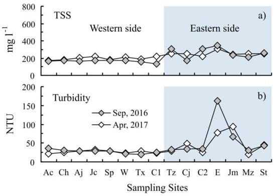
Figure 5.
Ground-based data taken in this study. (a) Total suspended solids (TSS) and, (b) turbidity quantifications (locations shown in Figure 1).
Taking into account the non-normal data distribution, similarities of the TSS and turbidity variations between seasons or areas of the lake were explained by the level association determined by the Spearman’s test (r2 = 0.51, p < 0.5). They were in accordance with the NWC dataset, which suggests a direct relationship between TSS and turbidity; but also highlighting the eastern side of the lake as the area of the major TSS concentrations and turbidity quantifications. Given these results, the fifteen sites considered in this study were used to calibrate the remote sensing-based model for turbidity; therefore, second-order polynomial regressions were employed to the model calibration between the NIR-reflectance and turbidity, obtaining a seasonal approach of the water turbidity in Lake Chapala. On the other hand, the NWC dataset was used to evaluate the model response.
3.3. Spectral Analysis
3.3.1. Sun-Glint Effect Removal
The sun-glint correction (SGC) applied to the fourteen Landsat-8 images enhanced the response from the water-leaving irradiance reflectance in Lake Chapala. From this dataset, two images corresponding to the survey dates were used to show the advantages of spectral improvement. The first was taken during the summer-fall season (06 September 2016), it was acquired the same day of the field sampling; while, the other was taken at the spring season (18 April 2017), six days before the second sampling date. This procedure allowed the balance of radiometric data in the VIS-NIR region, attenuating the reflectance surplus of the sun-glint effect from the water surface described by Kay et al. [67]. The removal of the sun-glint effect was statistically manifested in the histogram redistribution; the typical negative-skewness or bimodal frequency arrangement observed in Lake Chapala before the SGC was adjusted to a quasi-normal distribution, equalizing all data (Figure 6a–d).
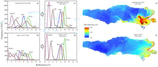
Figure 6.
Spectral histograms of the VIS-NIR-SWIR surface reflectance from Landsat-8: (a) corresponds to 6 September 2016, (b) corresponds to 18 April 2017. Histograms after the sun-glint correction (SGC) procedure: (c) for image taken on 6 September 2016 and (d) for image taken on 18 April 2017; water-leaving reflectance after the SGC: (e) 6 September 2016, and (f) corresponds to 18 April 2017.
Special attention deserves the NIR and Red bands of the two contemporaneous Landsat-8 images with the ground-based data. After the SGC, the image on 6 September 2016, exposed skewed histograms of the bands with a benched form along with the higher values, opposite to the image taken on 18 April 2017. These graphical benches corresponded to the water response related to sediment discharge events into the south and eastern side of the lake (Figure 6e,f).
3.3.2. Reflectance Retrieved from the Turbid Water
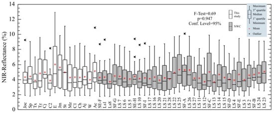
After the SGC, the water-leaving irradiance reflectance obtained from NIR-band of the fourteen Landsat-8 images was assessed taking into account the geographical position of the 34 sites from the NWC and 15 sites from the present study. It was found that the bulk of the reflectance values varied in the range of 2.5 to 8.5% (almost all into the first order). The analysis of variance of the reflectance showed that there were no significant differences among the medians of the 49 sites (p = 0.947) (Figure 7). Despite such similarities, the reflectance was slightly higher and more variable besides the Lerma River and La Pasión Creek (Tz. Jm, St, E, LS 22, LS 25, LS 26).
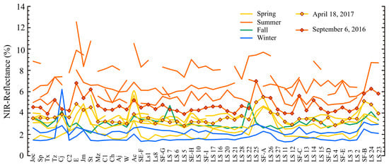
On the other hand, temporal changes of the NIR-reflectance showed an inter-annual variation. The statistical analysis indicates significant differences among the NIR-reflectance at distinct dates (p = 0), highlighting seasonal contrasts (Figure 8). The highest reflectance values of the summer season exceed the maximum limit of ~5% observed in the other seasons (Figure 9), becoming heterogeneous and more variable measurements among sites. They are opposite to the lowest reflectance values of the winter.
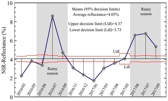
Figure 8.
NIR-reflectance inter-annual variation, highlighting the seasonal contrasts between summer and winter seasons.
3.4. Empirical Models for Turbidity
3.4.1. Calibration
Given the seasonal variations of the water-leaving-irradiance reflectance from the sub-surface level of the lake, wide ranges of values are required to consider all the possible values in the process of the model calibration; unfortunately, the coverage of the ground data was limited to a pair of sampling dates per year, restricting the temporal analysis to the sampling dates. In this sense, the model calibration was based on correlation functions between the NIR-reflectance and turbidity to obtain a seasonal approach of the water turbidity in the lake. Several functions were carried out to looking for the best empirical model, five images in the period March-2016 to September-2017 were identified close to the dates of the NWC and this study on-field data; six models were established between the contemporary data sources (Table 3). Almost all models followed a non-linear form (second-order polynomial), except for those carried out with the image taken on 4 May 2017 (linear).
Table 3.
Elements and criteria to carry out the model calibration.
The analysis of variance indicates that the functions based on the NWC data had a statistically significant relationship (except for June 2016); nevertheless, their relationships were the weakest among all (r2 < 0.63) (Table 3). The relationship between the image taken on May 4 and the NWC-survey data of 24 April 2016, stands out as the better relationship (r2 = 0.92); unfortunately, the models associated with this image were omitted of the model-construction process, due to after the SGC process only a limited lake surface was free of the sun-glint effect; consequently, a small number of sampling sites had a good correspondence with the NIR-reflectance estimations. Instead, the functions based on this study had strong relationships (r2 > 0.70), explaining a non-linear behavior between the NIR-reflectance and turbidity (Figure 10).
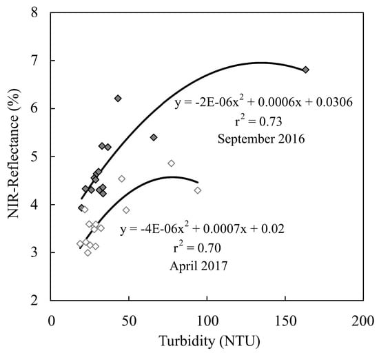
Figure 10.
Functions of correlation between the NIR-reflectance and turbidity.
Important differences were found between the correlation strength of this study and the NWC-derived models; the temporal delays appear as the main difference factor after the radiometric image improvements. Particularly, our samplings were conducted in one day (every one of them) with hourly temporal differences to the satellite overpass time during September 2016 and six days in the case of April 2017; while the NWC samplings were carried out during several days (even more than one week) and the temporal differences respect to the satellite-overpass were from 4 to 12 days. Additionally, the measurement range (400–600 nm) performed by the NWC was a factor that implicitly induced important deviations associated with organic matter; therefore, temporal delays and methodological approach have affected the relationships between the NIR reflectance and NWC turbidity measurements. After these considerations, the functions associated with our datasets were chosen to calibrate the empirical models for turbidity (Equation (1) for the summer-fall season, Equation (2) for the spring season).
The equations take the coefficients derived from the non-linear functions, considering the NIR reflectance (ρNIR) as the variable which determines the turbidity estimation.
3.4.2. Validation
The model validation was carried out to know their prediction capacity; therefore, the Equations (1) and (2) were applied to the Landsat-8 images taken close to the NWC surveys dates (9 September 2017, and 4 May 2017, respectively, Table 3). It was found that the turbidity estimations derived from Equation (1) and Equation (2), explained the 59 and 70% of the NWC-turbidity variation respectively (Figure 11a).
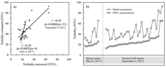
Figure 11.
(a) Turbidity-prediction empirical models; (b) absolute model deviations.
The model for the spring season estimated the water turbidity with the major prediction capacity (70%). These values were acceptable; however, such results were limited to a small lake surface, leaving them linked to a high dependence on the limited number of sampling sites. Otherwise, the model for the summer-fall season estimates the turbidity in a larger surface based on a major number of sampling sites (31 of 34). Its prediction capacity on the image taken in 2017 (September 9) was low to moderate (~60%) with a root mean square error (RMSE) of 23.6%; a similar RMSE (21.6%) obtained from the prediction carried out on the image taken on 6 September 2016.
Independently of the model adjustment, the location, the magnitude, the turbidity deviations between the model and the NWC and this study measurement were manifested as important model overestimations, which were of the order of two times itself turbidity value in some sites (Figure 11b).
4. Discussion
4.1. The Principal Turbidity Sources
The historical NWC data have shown TSS is the primary source of turbidity instead of the Chl a in Lake Chapala; such results led us to evaluate the TSS-turbidity relationships. The TSS and turbidity expose a similar spatial distribution; especially the mean values, which in both cases are sustained by the low standard error (less than 8%) in almost all the lake. The high certainty-percentage in the mean values of TSS and turbidity gives strong support to their spatial behavior; which explains the predominant sediment contribution of the Lerma river at the eastern side [36,74]. On the other side, the maximum values of both parameters exposed moderate to high uncertainties of the model prediction. Despite the high SE, it could be interpreted as normal spatial uncertainty due to the maximum values are related to low-frequency events which become especial cases, but also possible in the medium term, like in the case of the concentrations measured on 6 September 2016, and 24 April 2017.
4.2. Advantages and Challenges
The development of empirical models was based on the conventional methodology described by Matthews [11]. Two field surveys carried out in this study exposed spatial and seasonal conformity respect to the NWC turbidity quantifications on the same seasons; such similarities were fundamental to provide support to the model assessment, especially when the model validation was based on both datasets.
Otherwise, the Landsat-8 images represent the other data source; they were reviewed before the calibration procedure. The scientific community has improved methodologies to overcome the atmospheric interference at different satellite platforms [15,18,19,68,69,75]; nevertheless, the individual efforts do not ensure the image standardization to generate spectral analysis with comparable satellite scenes through the time, such as the surface reflectance approach of the Landsat constellation. The LaSRC proposed by Vermote et al. [61] and applied to the Landsat products involves great advantages for improving the surface reflectance measurements (with minimal environmental interference) but also facilitating the data management. This becomes an invaluable resource that we used to carry out a better approach in the turbidity estimations.
A secondary post-processing procedure was applied in fourteen Landsat-8 images (period March 2016 to September 2017) to enhance the retrieval of the water turbidity. The SGC method described by Lyzenga et al. [17] further improved the quality of the LaSRC surface reflectance images respect to optical artifacts at the water surface, normalizing the water-leaving irradiance reflectance response. This method cleared the way to carry out subsequent stages of processing to monitoring the permanent water turbidity that predominates in the lake [74], or the assessment of eventual clay discharges to the lake without the sun-glint.
These methodological improvements contribute to enhance the model response, but other factors are affecting the model construction. The LaSRC has solved geometrical artifacts [64,65] related to the bidirectional reflectance effects; however, the NIR-reflectance showed temporary variations, which are most likely associated with the incoming solar energy. In this case, the water-leaving irradiance reflectance showed an annual cyclical-pattern through the period 2016–2017, with higher percentages of reflectance during the rainiest months, and the lowest reflectance in the winter season. Particularly, the water-leaving irradiance reflectance in the spring and summer-fall seasons would be interpreted as the same; however, every season has different climatic conditions. The seasonal variations and similarities of the NIR-reflectance follow a normal behavior that matches with the incoming solar irradiation temporal pattern in this region, which is characterized by normal increases in the summer season [76]; nevertheless, the temporal randomness of the rain and cloud cover distribution affects the normality of the solar irradiation availability on the water surface. Therefore, each turbidity model was limited and probed upon image taken in the own season and close to the ground-sampling dates.
4.3. Time Delays Implications
The empirical models tend to have a limited ability to distinguish the signal of different covariant water parameters [11]; however, in the case of water turbidity, the optical interferences among organic and inorganic compounds in the NIR range become minimal or null [59]. This approach gives us the advantage to retrieve the water response without the absorption effect produce by the Colored Dissolved Organic Matter (CDOM); nevertheless, the findings derived from this study lead us to suggest the temporal delays as the main factor inducing the model uncertainty. Since the empirical model construction strongly depends on the high level of synchronization between the sampling and satellite overpass, as well as a great number of ground-based data to the calibration, it is reasonable to understand the moderate model approach, even when the calibration was related to hourly temporal delays.
In light of the findings, we can say that temporary variations (seasonal, daily or hourly) become a determining factor, indicating that a single empirical model would be deficient to explains the turbidity variations along the year, especially when limited number of dates were considered to its construction. Instead, an empirical model seems to be a reasonable alternative to explain the water turbidity in a particular season. More important is the fact of having synchronized satellite and field measurements to reduce the model calibration uncertainties. The obtaining of the broadest range of possible synchronized turbidity measurements into the lake would lead us to build a robust empirical model, enough to improve accurate turbidity diagnoses.
4.4. Model Interpretations
The empirical model turbidity for the summer-fall season (Equation (1)) offers a great opportunity to understand the hydrocyanic complexity in Lake Chapala. Despite its uncertainty, the empirical model applied to the images corresponding to September of 2016 and 2017 showed detailed spatial turbidity changes better than the geostatistical approach (Figure 12). The two model approaches draw a similar spatial distribution of the turbidity. Nevertheless, their estimations are exposed to different spatial resolutions, giving two different perspectives about this water parameter.
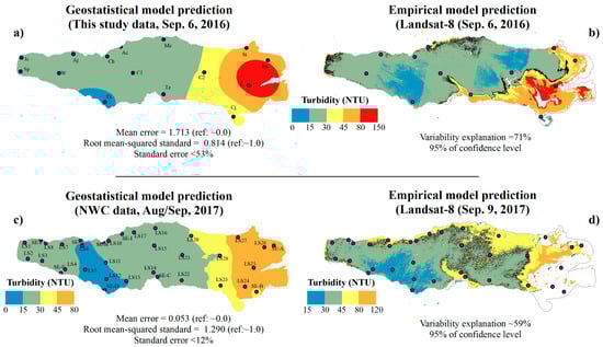
Figure 12.
Comparison between models, turbidity predictions during the summer-fall season. (a) Geostatistical model prediction based on this study measurements, (b) Empirical model estimated with Equation (1) and Landsat-8 for 6 September 2016, (c) Geostatistical model prediction based on NWC measurements, and (d) Empirical model estimated with Equation (1) and Landsat-8 for 9 September 2017.
The geostatistical models expose great surfaces without significant changes along to large distances; these models characterize a low horizontal gradient among the normal and atypical turbidity quantifications, hiding the steeped changes of turbidity in short distances, its sources, and the pathway through the lake. While the empirical model offers an instantaneous perspective of the continuous medium, allowing the recognition of the turbidity horizontal-changes every 30 m. These model-advantages helped us to identify the sharp turbidity change above the 30 NTU in a strip extended along the east, southeast and northeast areas of the lake (Figure 12b,d). This spatial feature identifies a transitional boundary where the horizontal gradient of turbidity abruptly begin to increase in the east direction; dividing the lake turbidity in two great areas, the first at the center and western side with low turbidity (less than 30 NTU), and the second with high turbidity values (up to ~150 NTU) along the shoreline and the deltaic structure of the Lerma river in the eastern side of the lake. Particularly in the last area, the model highlights the clay sediments-related turbidity from discharges of the main rivers, as well as increases in the water turbidity along the shoreline adjacent to the largest population centers, which are located around the lake where important industrial, agricultural or tourism activities are very common (Figure 1).
The causes of the high turbidity in the eastern side of the lake are beyond the aims of this study; however, our preliminary result would provide some insights to understand the water dynamics and the factors inducing turbidity in Lake Chapala. We could say the high turbidity values on the eastern side mainly appears to be determined by river discharges. Several sediment plumes were detected with the empirical model, arising hydrodynamic features of the lake. The model exhibits the origin of currents from the Santiago river, highlighting changes in the natural direction of the water flow explained by Fernex et al. [77]. Other currents were detected from the Lerma River and La Pasión Creek, evidencing the extensive erosion processes generated in their catchments and the sediment transport to the lake [45,46,47]. However, the finding of the spatial strip along the eastern side of the lake suggests that high turbidity values in this area furthermore respond to other factors that produce a sudden increase in the horizontal rate of turbidity values at short distances. The shallow waters enclosed into a couple of cove beside the Lerma-outlet house the higher turbidity values; their shoreline morphology and the bathymetry related to the deltaic structure in this area appears to be an appropriate environment in which the water column height, physical phenomena such as the vertical temperature gradient, internal waves movement and the wind shear-stress [39,40] induce the higher turbidity into the lake.
The satellite approach and the improvement of empirical models become complementary alternatives to monitoring the water turbidity; in this case, the satellite-based model contributes to display an instantaneous image of the spatial pattern of turbidity in Lake Chapala. Nevertheless, more research should be done to improve more robust empirical models to get major predictability on the water assessment; and consequently, to reach a better capacity to elucidate the influence of environmental factors on the turbidity into the lake, such as the lake morphology or water hydrodynamic.
5. Conclusions
The high quality of the LaSCR surface reflectance images from Landsat-8 further was improved with a statistical algorithm to remove the sun-glint contamination in the VIS-NIR region. These image improvements lead us to retrieve the water turbidity from the lake with greater accuracy. A set of fourteen images taken along the inter-annual cycle 2016–2017 were processed to develop a suitable empirical model for turbidity in Lake Chapala (Mexico). Several models were tested on the water-leaving irradiance reflectance from the NIR band and in-situ turbidity relationships. It was expected a strong empirical model calibration based on the field information; however, most of the relationships were weak. All of them were associated with daily delays and a small number of sampling sites; while, few functions showed an appropriate adjustment, among them a model based on hourly data, exposing the better empirical approach to predict the turbidity only for the summer-fall season.
Some interpretations derived from this model suggest that in addition to the river discharges, the hydrodynamic and morphologic features induce remarkable turbidity in the eastern side of the lake, all following the historical records. Moreover, the instantaneous images derived from the model depict the complexity of the water movement patterns in the lake, which involve a strong component of spatial randomness inherently associated with the temporal delays, contributing to the model deviation. Therefore, a strong empirical model should be based on a great number of sampling sites and dates synchronized with the satellite overpass to explain the turbidity and its impacts in dynamic and shallow aquatic environments of subtropical zones such as Lake Chapala.
Author Contributions
P.O.: Conceptualization, Investigation, Methodology, Software, Formal analysis, Writing. R.V.-R.: Resources, Formal analysis, Validation, Writing, Funding acquisition, Project administration. S.K.: Supervision, Writing. E.L.-B.: Project administration, Writing. J.d.A.: Resources, Writing. L.H.-M.: Methodology, Formal analysis, Writing. J.d.R.-O.: Writing. J.d.J.D.-T.: Conceptualization, Investigation, Methodology, Resources, Software, Formal analysis, Validation, Visualization, Writing, Project administration. All authors have read and agreed to the published version of the manuscript.
Funding
This research was funded by the National Council of Science and Technology of Mexico (Consejo Nacional de Ciencia y Tecnología, CONACYT by its acronym in Spanish), grant number 248408-PDCPN2014-01.
Acknowledgments
We would like to thank the National Water Council by the water quality data, to the National Meteorological Survey in Mexico by the meteorological data; to the State Water Council in Jalisco by bathymetrical information; as well as the United States Geological Survey by the Landsat-8 and SRTM-topography data. We also want to thanks the students Leonardo Martínez by their support in the field sampling and laboratory activities.
Conflicts of Interest
The authors declare no conflict of interest. The funders had no role in the design of the study; in the collection, analyses, or interpretation of data; in the writing of the manuscript, or in the decision to publish the results.
References
- Chapman, D.V. Water Quality Assessments: A Guide to the Use of Biota, Sediments and Water in Environmental Monitoring, 2nd ed.; University Press: Cambridge, UK, 1996. [Google Scholar]
- Chapin, F.S., III; Zavaleta, E.S.; Eviner, V.T.; Naylor, R.L.; Vitousek, P.M.; Reynolds, H.L.; Hooper, D.U.; Lavorel, S.; Sala, O.E.; Hobble, S.E.; et al. Consequences of changing biodiversity. Nature 2000, 405, 234. [Google Scholar] [CrossRef]
- Williams, P.; Whitfield, M.; Biggs, J.; Bray, S.; Fox, G.; Nicolet, P.; Sear, D. Comparative biodiversity of rivers, streams, ditches and ponds in an agricultural landscape in Southern England. Biol. Conserv. 2004, 115, 329–341. [Google Scholar] [CrossRef]
- Oertli, B.; Biggs, J.; Céréghino, R.; Grillas, P.; Joly, P.; Lachavanne, J.B. Conservation and monitoring of pond biodiversity: Introduction. Aquat. Conserv. Mar. Freshw. Ecosyst. 2005, 15, 535–540. [Google Scholar] [CrossRef]
- Wetzel, R.G. Limnology: Lake and River Ecosystems, 3rd ed.; Elsevier Academic Press: Amsterdam, The Netherlands, 2001; p. 1006. ISBN -13: 978-0-12-744760-5. [Google Scholar]
- Bastin, J.F.; Clark, E.; Elliott, T.; Hart, S.; Van den Hoogen, J.; Hordijk, I.; Ma, H.; Majumder, S.; Manoli, G.; Maschler, J.; et al. Understanding climate change from a global analysis of city analogues. PLoS ONE 2019, 14, e0217592. [Google Scholar]
- Zaneveld, J.R.V. A theoretical derivation of the dependence of the remotely sensed reflectance of the ocean on the inherent optical properties. J. Geophys. Res. Ocean 1995, 100, 13135–13142. [Google Scholar] [CrossRef]
- Dekker, A.G.; Hoogenboom, H.J.; Goddijn, L.M.; Malthus, T.J.M. The relation between inherent optical properties and reflectance spectra in turbid inland waters. Remote Sens. Rev. 1997, 15, 59–74. [Google Scholar] [CrossRef]
- Dekker, A.G.; Vos, R.J.; Peters, S.W.M. Comparison of remote sensing data, model results and in situ data for total suspended matter (TSM) in the southern Frisian lakes. Sci. Total Environ. 2001, 268, 197–214. [Google Scholar] [CrossRef]
- Doxaran, D.; Ehn, J.; Bélanger, S.; Matsuoka, A.; Hooker, S.; Babin, M. Remote sensing the dynamics of suspended particles in the Mackenzie river plume (Canadian Arctic Ocean). Biogeosci. Discuss. 2012, 9, 5205–5248. [Google Scholar] [CrossRef]
- Matthews, M.W. A current review of empirical procedures of remote sensing in inland and near-coastal transitional waters. Int. J. Remote Sens. 2011, 32, 6855–6899. [Google Scholar] [CrossRef]
- Lathrop, R.G.; Lillesand, T.M. Monitoring water quality and river plume transport in Green Bay, Lake Michigan with SPOT-1 imagery. Photogramm. Eng. Remote Sens. 1989, 55, 349–354. [Google Scholar]
- Harrington, J.A., Jr.; Schiebe, F.R.; Nix, J.F. Remote sensing of Lake Chicot, Arkansas: Monitoring suspended sediments, turbidity, and Secchi depth with Landsat MSS data. Remote Sens. Environ. 1992, 39, 15–27. [Google Scholar] [CrossRef]
- Härmä, P.; Vepsäläinen, J.; Hannonen, T.; Pyhälahti, T.; Kämäri, J.; Kallio, K.; Eloheimo, K.; Koponen, S. Detection of water quality using simulated satellite data and semi-empirical algorithms in Finland. Sci. Total Environ. 2001, 268, 107–121. [Google Scholar] [CrossRef]
- Doxaran, D.; Froidefond, J.M.; Lavender, S.; Castaing, P. Spectral signature of highly turbid waters: Application with SPOT data to quantify suspended particulate matter concentrations. Remote Sens. Environ. 2002, 81, 149–161. [Google Scholar] [CrossRef]
- Hedley, J.D.; Harborne, A.R.; Mumby, P.J. Simple and robust removal of sun glint for mapping shallow-water benthos. Int. J. Remote Sens. 2005, 26, 2107–2112. [Google Scholar] [CrossRef]
- Lyzenga, D.R.; Malinas, N.P.; Tanis, F.J. Multispectral bathymetry using a simple physically based algorithm. IEEE Trans. Geosci. Remote Sens. 2006, 44, 2251–2259. [Google Scholar] [CrossRef]
- Nechad, B.; Ruddick, K.G.; Park, Y. Calibration and validation of a generic multisensor algorithm for mapping of total suspended matter in turbid waters. Remote Sens. Environ. 2010, 114, 854–866. [Google Scholar] [CrossRef]
- Dogliotti, A.I.; Ruddick, K.G.; Nechad, B.; Doxaran, D.; Knaeps, E. A single algorithm to retrieve turbidity from remotely-sensed data in all coastal and estuarine waters. Remote Sens. Environ. 2015, 156, 157–168. [Google Scholar] [CrossRef]
- Kallio, K.; Attila, J.; Härmä, P.; Koponen, S.; Pulliainen, J.; Hyytiäinen, U.M.; Pyhälahti, T. Landsat ETM+ images in the estimation of seasonal lake water quality in boreal river basins. Environ. Manag. 2008, 42, 511–522. [Google Scholar] [CrossRef]
- Kloiber, S.M.; Brezonik, P.L.; Bauer, M.E. Application of Landsat imagery to regional-scale assessments of lake clarity. Water Res. 2002, 36, 4330–4340. [Google Scholar] [CrossRef]
- Vincent, R.K.; Qin, X.; McKay, R.M.L.; Miner, J.; Czajkowski, K.; Savino, J.; Bridgeman, T. Phycocyanin detection from LANDSAT TM data for mapping cyanobacterial blooms in Lake Erie. Remote Sens. Environ. 2004, 89, 381–392. [Google Scholar] [CrossRef]
- Tyler, A.N.; Svab, E.; Preston, T.; Présing, M.; Kovács, W.A. Remote sensing of the water quality of shallow lakes: A mixture modelling approach to quantifying phytoplankton in water characterized by high-suspended sediment. Int. J. Remote Sens. 2006, 27, 1521–1537. [Google Scholar] [CrossRef]
- Hicks, B.J.; Stichbury, G.A.; Brabyn, L.K.; Allan, M.G.; Ashraf, S. Hindcasting water clarity from Landsat satellite images of unmonitored shallow lakes in the Waikato region, New Zealand. Environ. Monit. Assess. 2013, 185, 7245–7261. [Google Scholar] [CrossRef] [PubMed]
- Barrett, D.C.; Frazier, A.E. Automated method for monitoring water quality using Landsat Imagery. Water 2016, 8, 257. [Google Scholar] [CrossRef]
- Barbosa, C.C.F.; Novo, E.M.L.M.; Martinez, J.M. Remote sensing of the water properties of the Amazon floodplain lakes: The time delay effects between in-situ and satellite data acquisition on model accuracy. In International Symposium on Remote Sensing of Environment: Sustaining the Millennium Development Goals; International Center for Remote Sensing of Environment (ICRSE): Tucson, AZ, USA, 2009; Volume 33. [Google Scholar]
- Song, K.; Wang, Z.; Blackwell, J.; Zhang, B.; Li, F.; Zhang, Y.; Jiang, G. Water quality monitoring using Landsat Themate Mapper data with empirical algorithms in Chagan Lake, China. J. Appl. Remote Sens. 2011, 5, 053506. [Google Scholar] [CrossRef]
- Sheng, Y.P.; Lick, W. The transport and resuspension of sediments in a shallow lake. J. Geophys. Res. 1979, 84, 1809–1826. [Google Scholar] [CrossRef]
- Bloesch, J. Mechanisms, measurement and importance of sediment resuspension in lakes. Mar. Freshw. Res. 1995, 46, 295–304. [Google Scholar] [CrossRef]
- Chung, E.G.; Bombardelli, F.A.; Schladow, S.G. Sediment resuspension in a shallow lake. Water Resour. Res. 2009, 45. [Google Scholar] [CrossRef]
- United State Environmental Protection Agency (USEPA). Monitoring Water Quality, Volunteer Stream Monitoring: A Methods Manual; Office of Water 841-B-97-003; United State Environmental Protection Agency (USEPA): Washington, DC, USA, 1997; 214p.
- Secretary of Health in Mexico (Secretaría de Salud). Diario Oficial de la Federación. NOM-127-SSA1-1994. 1995. Available online: http://www.salud.gob.mx/unidades/cdi/nom/127ssa14.html (accessed on 25 December 2019).
- World Health Organization (WHO). Guidelines for Drinking-Water Quality Criteria and Other Supporting Information International Programme on Chemical Safety, 2nd ed.; World Health Organization (WHO): Geneva, Switzerland, 1996; Volume 2, 94p. [Google Scholar]
- Eurpoean Union. Directive 2008/56/EC of the European Parliament and of the Concil of 17 June 2008 establishing a Framework for Community Action in the Field of Marine Environmental Policy (Marine Estrategy Framework Directive). Off. J. Eur. Union 2008, 164, 19–40. [Google Scholar]
- USEPA. Federal Water Pollution Control Act Amendments of, Part 125―Criteria and Standards for the National Pollutant Discharge Elimination System; Code of Federal Regulations, Title 40; United State Environmental Protection Agency (USEPA): Washington, DC, USA, 1972; Volume 21, Chapter I, Sub-Chapter D (Water Programs). [Google Scholar]
- Lind, O.T.; Doyle, R.; Vodopich, D.S.; Trotter, B.G.; Limón, J.G.; Davalos-Lind, L. Clay turbidity: Regulation of phytoplankton production in a large, nutrient-rich tropical lake. Limnol. Oceanogr. 1992, 37, 549–565. [Google Scholar] [CrossRef]
- Limón-Macías, J.G.; Lind, O.T. The management of Lake Chapala (Mexico): Considerations after significant changes in the water regime. Lake Reserv. Manag. 1990, 6, 61–70. [Google Scholar] [CrossRef]
- Lind, O.T.; Davalos-Lind, L.O. Interaction of water quantity with water quality: The Lake Chapala example. Hydrobiologia 2002, 467, 159–167. [Google Scholar] [CrossRef]
- Filonov, A.E.; Tereshchenko, I.E. Thermal lenses and internal solitons in Chapala Lake, Mexico. Chin. J. Oceanol. Limnol. 1999, 17, 308–314. [Google Scholar] [CrossRef]
- Filonov, A.E. On the dynamical response of Lake Chapala, Mexico to lake breeze forcing. Hydrobiologia 2002, 467, 141–157. [Google Scholar] [CrossRef]
- Ávalos-Cueva, D.; Filonov, A.; Tereshchenko, I.; Monzón, C.; Pantoja-González, D.; Velázquez-Muñoz, F. The level variability, thermal structure and currents in Lake Chapala, Mexico. Geofísica Int. 2016, 55, 175–187. [Google Scholar]
- Comisión Nacional del Agua (CONAGUA). Atlas del Agua en México; Secretaría de Medio Ambiente y Recursos Naturales: Mexico City, Mexico, 2016; 138p. [Google Scholar]
- Aparicio, J. Hydrology of the Lerma-Chapala Watershed. In The Lerma-Chapala Watershed; Hansen, A.M., van Afferden, M., Eds.; Springer: Boston, MA, USA, 2001. [Google Scholar] [CrossRef]
- De León-Mojarro, B.; Medina-Mendoza, R.; González-Casillas, A. Natural Resources Management in the Lerma-Chapala Basin. In The Lerma-Chapala Watershed; Hansen, A.M., van Afferden, M., Eds.; Springer: Boston, MA, USA, 2001. [Google Scholar] [CrossRef]
- Hansen, A.M.; van Afferden, M. Toxic Substances. In The Lerma-Chapala Watershed; Hansen, A.M., van Afferden, M., Eds.; Springer: Boston, MA, USA, 2001. [Google Scholar] [CrossRef]
- Jay, J.A.; Ford, T.E. Water Concentrations, Bioaccumulation, and Human Health Implications of Heavy Metals in Lake Chapala. In The Lerma-Chapala Watershed; Hansen, A.M., van Afferden, M., Eds.; Springer: Boston, MA, USA, 2001. [Google Scholar] [CrossRef]
- De Anda, J.; Shear, H.; Maniak, U.; Zárate del Valle, P.F. Solids distribution in Lake Chapala, Mexico. J. Am. Water Resour. Assoc. 2004, 40, 97–109. [Google Scholar] [CrossRef]
- Keesstra, S.; Nunes, J.P.; Saco, P.; Parsons, T.; Poeppl, R.; Masselink, R.; Cerdà, A. The way forward: Can connectivity be useful to design better measuring and modelling schemes for water and sediment dynamics? Sci. Total Environ. 2018, 644, 1557–1572. [Google Scholar] [CrossRef]
- Schalles, J.F. Optical remote sensing techniques to estimate phytoplankton, chlorophyll a concentrations in coastal. In Remote Sensing of Aquatic Coastal Ecosystem Processes; Richardson, L.L., LeDrew, E.F., Eds.; Springer: Dordrecht, The Netherlands, 2006; pp. 27–79. [Google Scholar]
- Rodríguez-Padilla, J.J. Desarrollo de un Sistema de Información Geográfica para el Análisis de Datos de Calidad de Agua del Lago de Chapala (México). Master’s Thesis, Instituto Tecnológico de Estudios Superiores de Monterrey, Guadalajara, Mexico, 2000; 112p. [Google Scholar]
- Membrillo-Abad, A.S.; Torres-Vera, M.A.; Alcocer, J.; Prol-Ledesma, R.M.; Oseguera, L.A.; Ruiz-Armenta, J.R. Trophic State Index estimation from remote sensing of lake Chapala, México. Rev. Mex. Cienc. Geol. 2016, 33, 183–191. [Google Scholar]
- APHA (American Public Health Association). Standard Methods for the Examination of Water and Wastewater, 22nd ed.; American Public Health Association; American Water Works Association; Water Environmental Federation: Washington, DC, USA, 2005. [Google Scholar]
- Peat, J.; Barton, B. Medical Statistics: A Guide to Data Analysis and Critical Appraisal; John Wiley & Sons: Hoboken, NJ, USA, 2008. [Google Scholar]
- Steinskog, D.J.; Tjøstheim, D.B.; Kvamstø, N.G. A cautionary note on the use of the Kolmogorov—Smirnov test for normality. Mon. Weather Rev. 2007, 135, 1151–1157. [Google Scholar] [CrossRef]
- Johnston, K.; Ver Hoef, J.M.; Krivoruchko, K.; Lucas, N. Using ArcGIS Geostatistical Analyst; ESRI: Redlands, CA, USA, 2001; Volume 380. [Google Scholar]
- Clark, I. Practical Geostatistics; Applied Science Publishers: London, UK, 1979; Volume 3, p. 129. [Google Scholar]
- Hongve, D.; Åkesson, G. Comparison of nephelometric turbidity measurements using wavelengths 400–600 and 860 nm. Water Res. 1998, 32, 3143–3145. [Google Scholar] [CrossRef]
- Mylvaganam, S.; Jakobsen, T. Turbidity sensor for underwater applications. In Proceedings of the OCEANS’98 Conference Proceedings, Nice, France, 28 September–1 October 1998; Volume 1, pp. 158–161. [Google Scholar]
- International Organization for Standards (ISO). International Standard ISO 7027—Water Quality—Determination of Turbidity—Part 1: Quantitative Methods; International Organization for Standards (ISO): Geneva, Switzerland, 2016. [Google Scholar]
- USGS (United States, Geological Survey). Landsat 8 Surface Reflectance Code (LaSRC) Product Guide; Earth Resources Observation and Science (EROS) Center: Sioux Falls, SD, USA, 2019; 98p.
- Vermote, E.; Justice, C.; Claverie, M.; Franch, B. Preliminary analysis of the performance of the Landsat 8/OLI land surface reflectance product. Remote Sens. Environ. 2016, 185, 46–56. [Google Scholar] [CrossRef]
- Morel, A.; Gentili, B. Diffuse reflectance of oceanic waters. III. Implication of bidirectionality for the remote-sensing problem. Appl. Opt. 1996, 35, 4850–4862. [Google Scholar] [CrossRef] [PubMed]
- Park, Y.J.; Ruddick, K. Model of remote-sensing reflectance including bidirectional effects for case 1 and case 2 waters. Appl. Opt. 2005, 44, 1236–1249. [Google Scholar] [CrossRef] [PubMed]
- Doerffer, R.; Schiller, H. The MERIS Case 2 water algorithm. Int. J. Remote Sens. 2007, 28, 517–535. [Google Scholar] [CrossRef]
- USGS. Landsat Surface Reflectance Data; USGS: Sioux Falls, SD, USA, 2015; Fact Sheet 2015–3034; 1p. Available online: https://doi.org/10.3133/fs20153034 (accessed on 25 June 2019).
- Chuvieco, E. Teledetección Ambiental, 3rd ed.; Editorial Ariel: Barcelona, Spain, 2010. [Google Scholar]
- Kay, S.; Hedley, J.D.; Lavender, S. Sun glint correction of high and low spatial resolution images of aquatic scenes: A review of methods for visible and near-infrared wavelengths. Remote Sens. 2009, 1, 697–730. [Google Scholar] [CrossRef]
- Stumpf, R.P.; Arnone, R.A.; Gould, R.W.; Martinolich, P.M.; Ransibrahmanakul, V. A partially coupled ocean-atmosphere model for retrieval of water-leaving radiance from SeaWiFS in coastal waters. NASA Tech. Memo. 2003, 206892, 51–59. [Google Scholar]
- Lavender, S.J.; Pinkerton, M.H.; Moore, G.F.; Aiken, J.; Blondeau-Patissier, D. Modification to the atmospheric correction of SeaWiFS ocean colour images over turbid waters. Cont. Shelf Res. 2005, 25, 539–555. [Google Scholar] [CrossRef]
- Wang, M.; Shi, W. The NIR-SWIR combined atmospheric correction approach for MODIS ocean color data processing. Opt. Express 2007, 15, 15722–15733. [Google Scholar] [CrossRef]
- Hale, G.M.; Querry, M.R. Optical constants of water in the 200-nm to 200-μm wavelength region. Appl. Opt. 1973, 12, 555–563. [Google Scholar] [CrossRef]
- Shi, W.; Wang, M. An assessment of the black ocean pixel assumption for MODIS SWIR bands. Remote Sens. Environ. 2009, 113, 1587–1597. [Google Scholar] [CrossRef]
- Lobo, F.L.; Costa, M.P.; Novo, E.M. Time-series analysis of Landsat-MSS/TM/OLI images over Amazonian waters impacted by gold mining activities. Remote Sens. Environ. 2015, 157, 170–184. [Google Scholar] [CrossRef]
- Lind, O.T.; Chrzanowski, T.H.; Dávalos-Lind, L. Clay turbidity and the relative production of bacterioplankton and phytoplankton. Hydrobiologia 1997, 353, 1–18. [Google Scholar] [CrossRef]
- Shi, W.; Wang, M. Detection of turbid waters and absorbing aerosols for the MODIS ocean color data processing. Remote Sens. Environ. 2007, 110, 149–161. [Google Scholar] [CrossRef]
- Díaz-Torres, J.J.; Hernández-Mena, L.; Murillo-Tovar, M.A.; León-Becerril, E.; López-López, A.; Suárez-Plascencia, C.; Aviña-Rodriguez, E.; Barradas-Gimate, A.; Ojeda-Castillo, V. Assessment of the modulation effect of rainfall on solar radiation availability at the Earth’s surface. Meteorol. Appl. 2017, 24, 180–190. [Google Scholar] [CrossRef]
- Fernex, F.; Zárate-del Valle, P.; Ramírez-Sánchez, H.; Michaud, F.; Parron, C.; Dalmasso, J.; Barci-Funel, G.; Guzman-Arroyo, M. Sedimentation rates in Lake Chapala (western Mexico): Possible active tectonic control. Chem. Geol. 2001, 177, 213–228. [Google Scholar] [CrossRef]


© 2019 by the authors. Licensee MDPI, Basel, Switzerland. This article is an open access article distributed under the terms and conditions of the Creative Commons Attribution (CC BY) license (http://creativecommons.org/licenses/by/4.0/).