Analyzing Space–Time Coherence in Precipitation Seasonality across Different European Climates


Abstract
1. Introduction
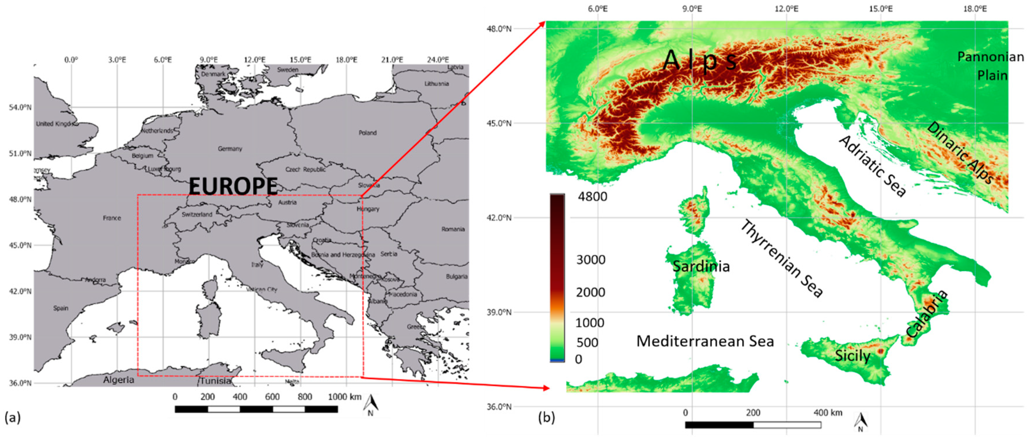
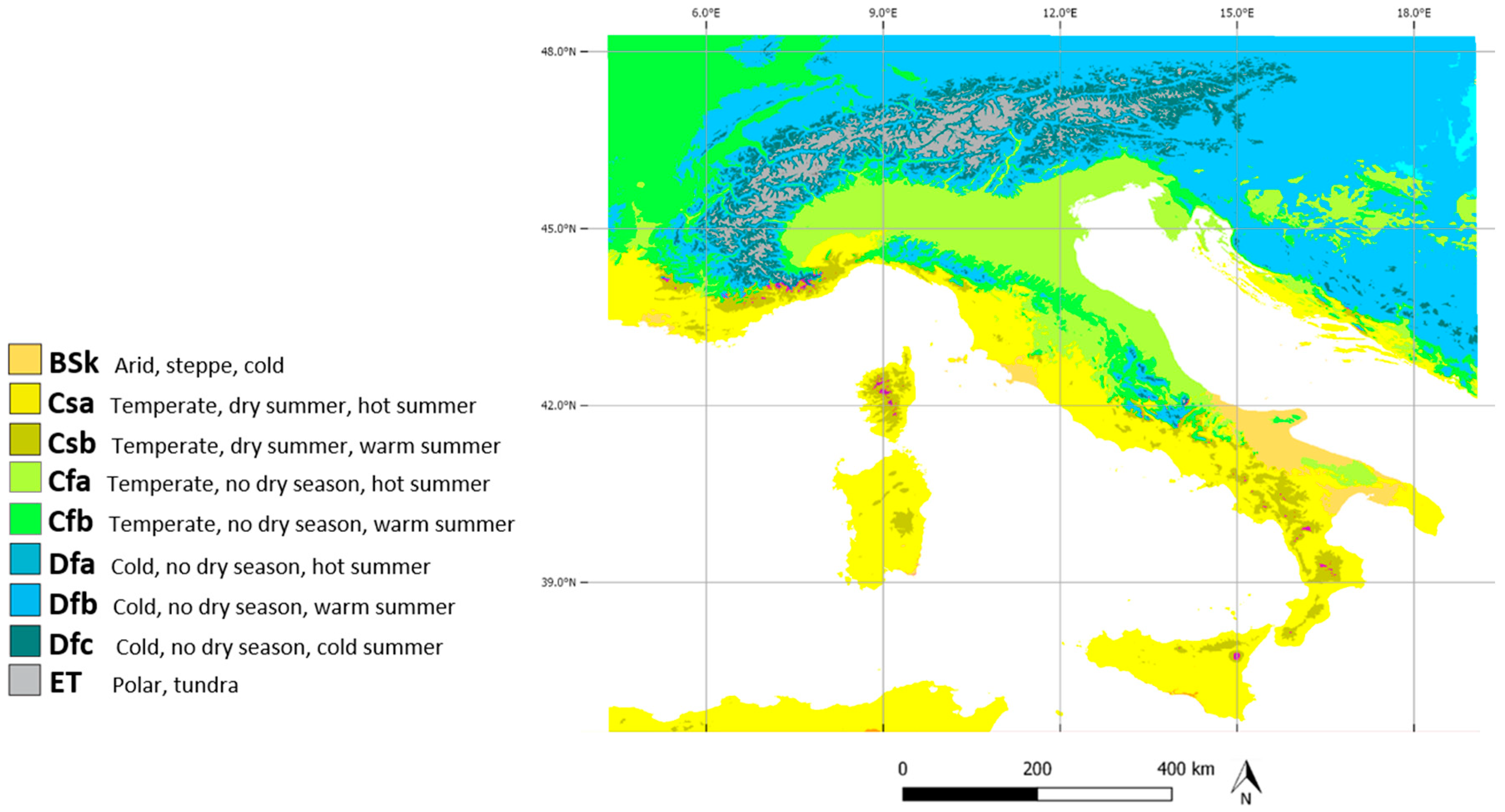
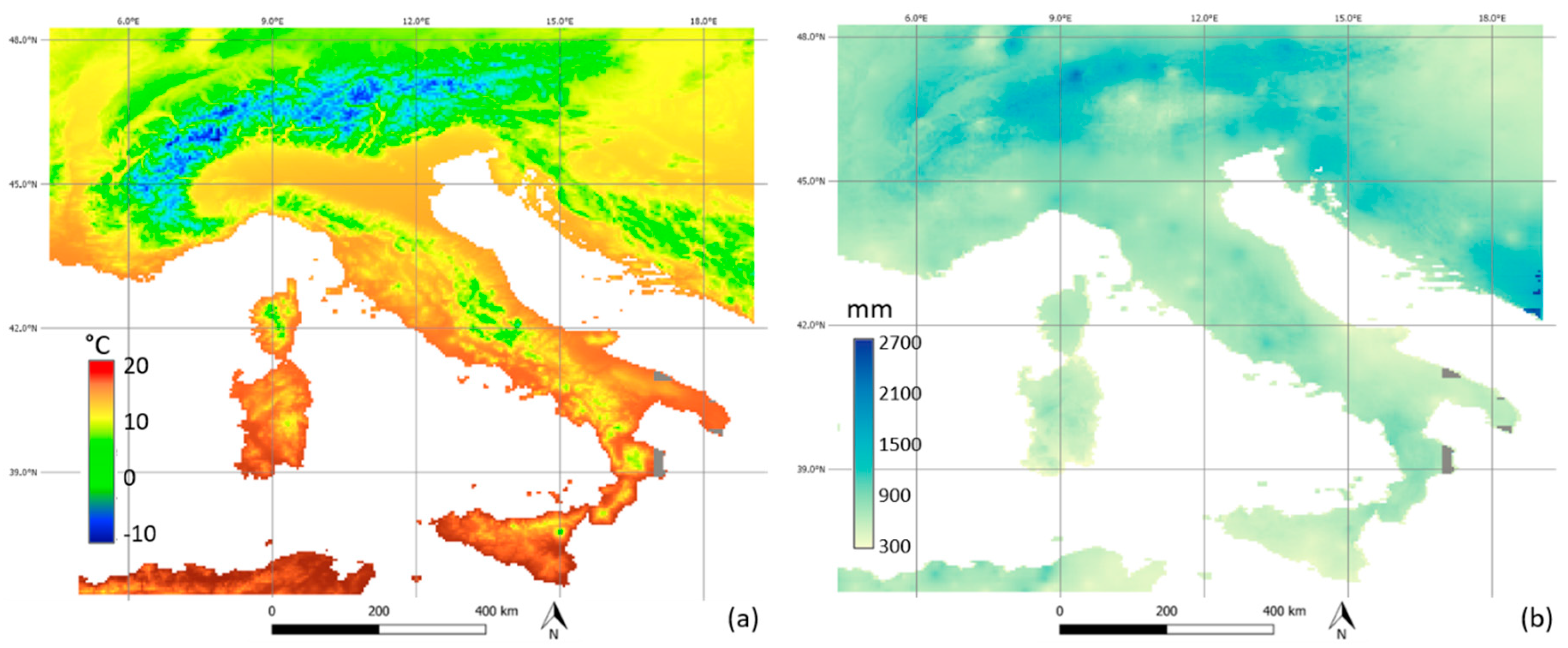
2. Study Area
3. Materials and Methods
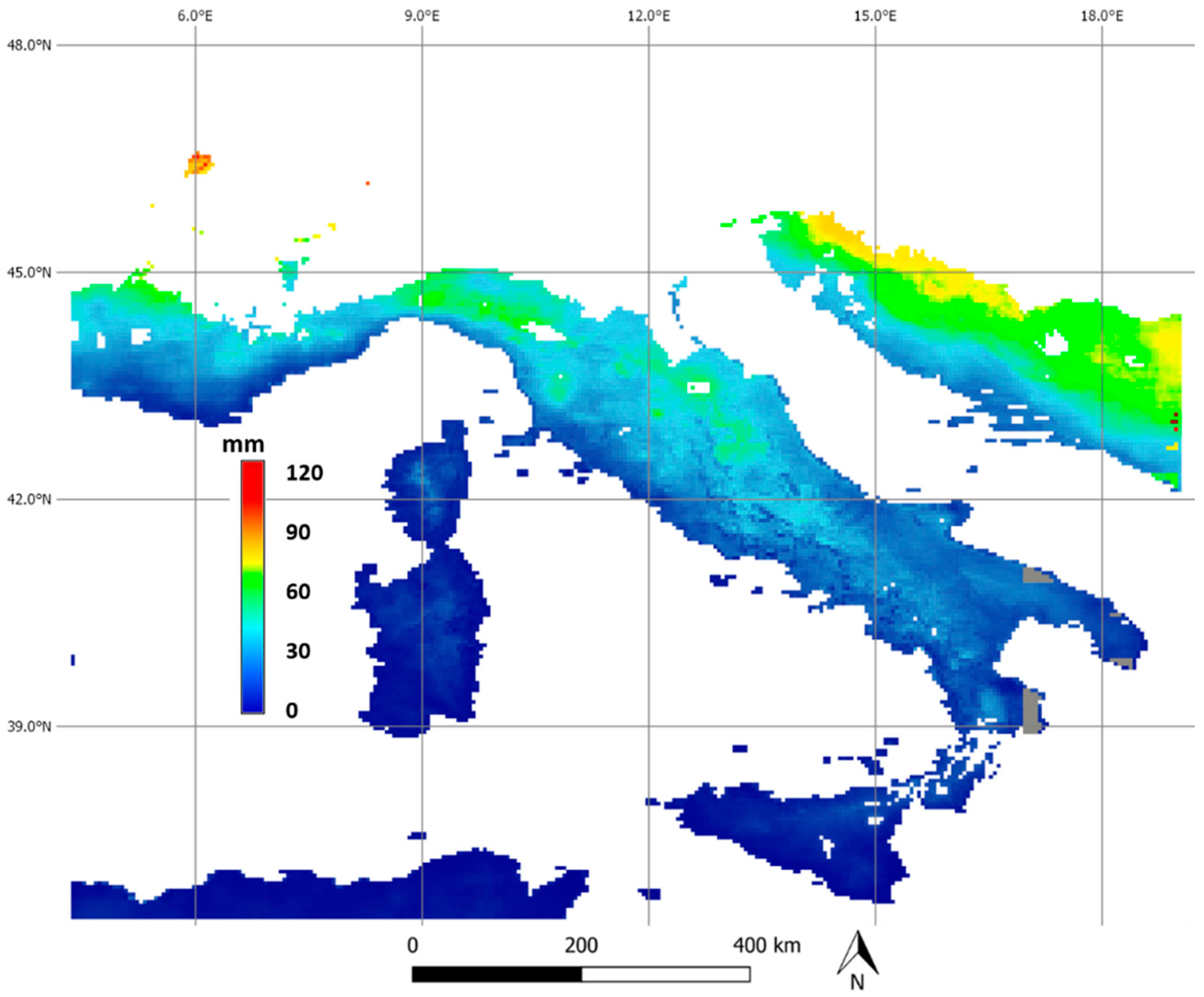
3.1. CHIRPS Data
- the monthly precipitation climatology, Climatology Climate Hazards Precipitation (CHPClim) [14];
- the in situ precipitation observations obtained from a variety of sources including national and regional meteorological services.
- rainfall from satellite data is estimated as the percentage of time during the pentad that the IR observation is lower than 235° K (cold cloud tops); this value is converted into millimeters of precipitation by means of previously determined local regression with TRMM 3B42 precipitation pentads. The IR pentads are then expressed as percent values of normal by dividing the values by their long-term (1981–2012) means.
- percent values of normal IR pentad are multiplied with the CHPClim in each pentad. Finally, this adjusted IR-retrieved precipitation is blended with surface gauges to produce the final product CHIRPS. Missing values due to incomplete satellite coverage are filled with CFSv2 data.
3.2. Cluster Analysis of Average Seasonal Patterns by K-means
4. Results and Discussion
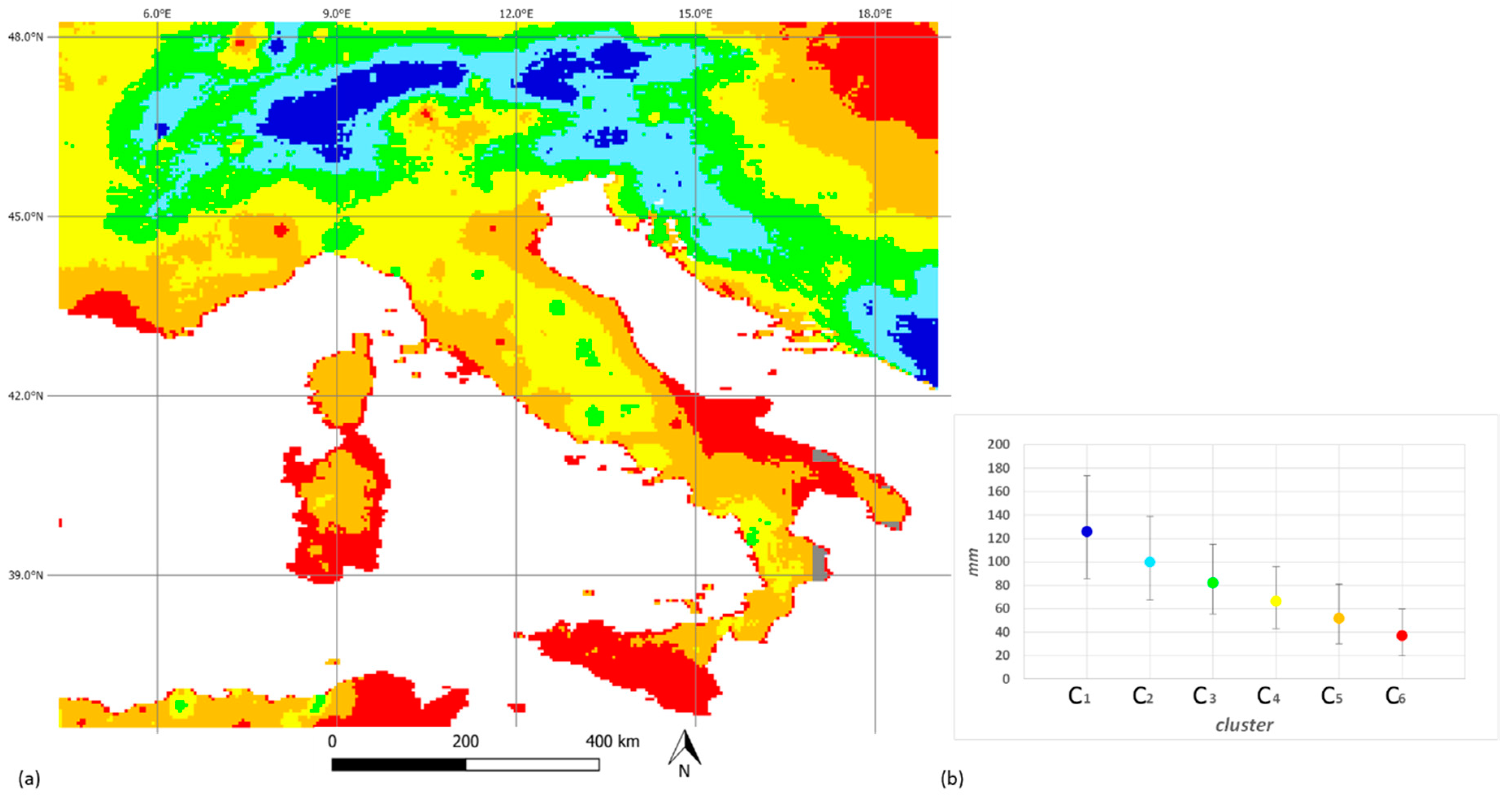
4.1. Cluster Analysis of Sample Time Distributions
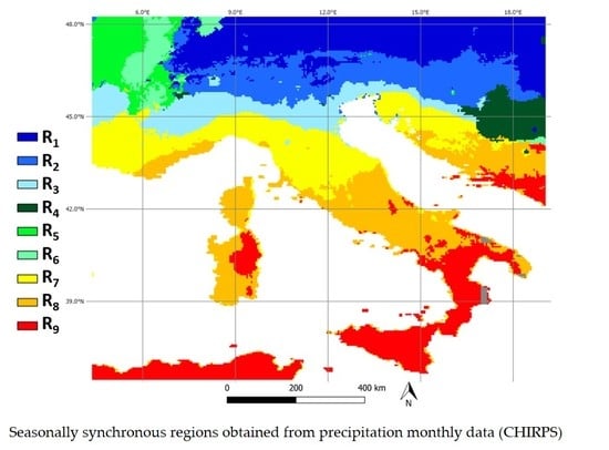
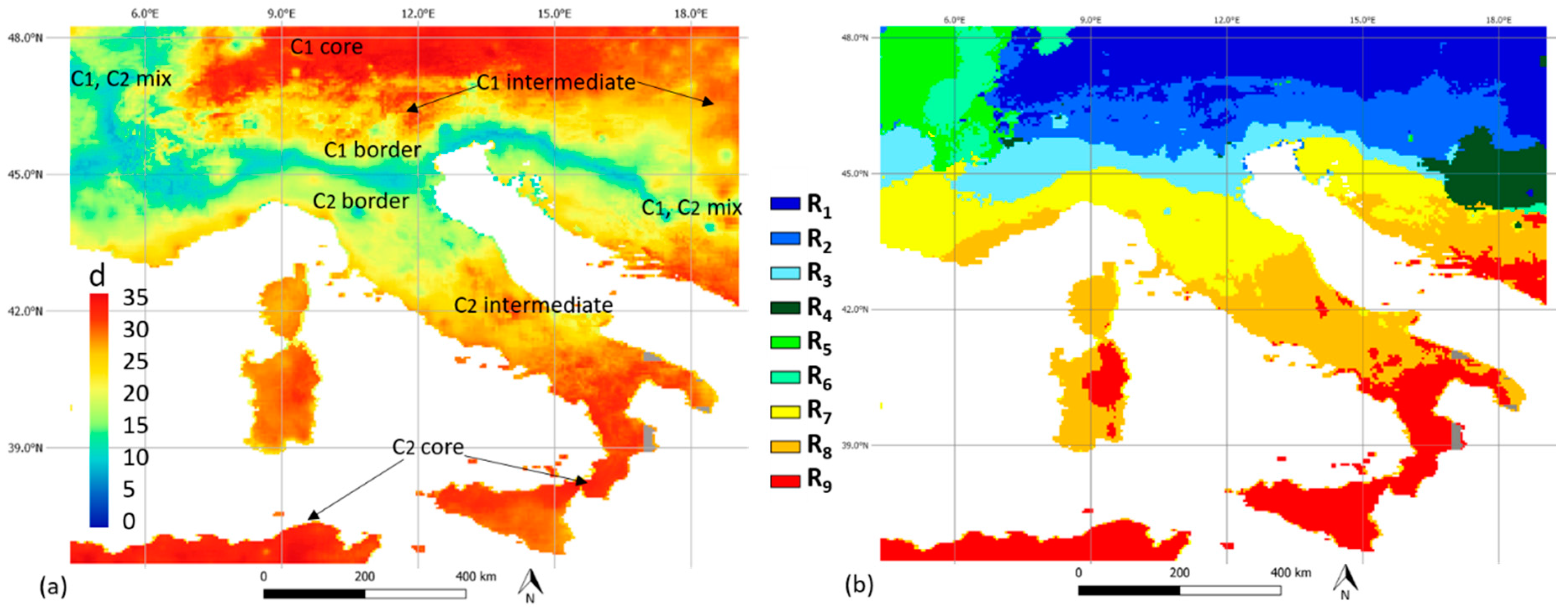
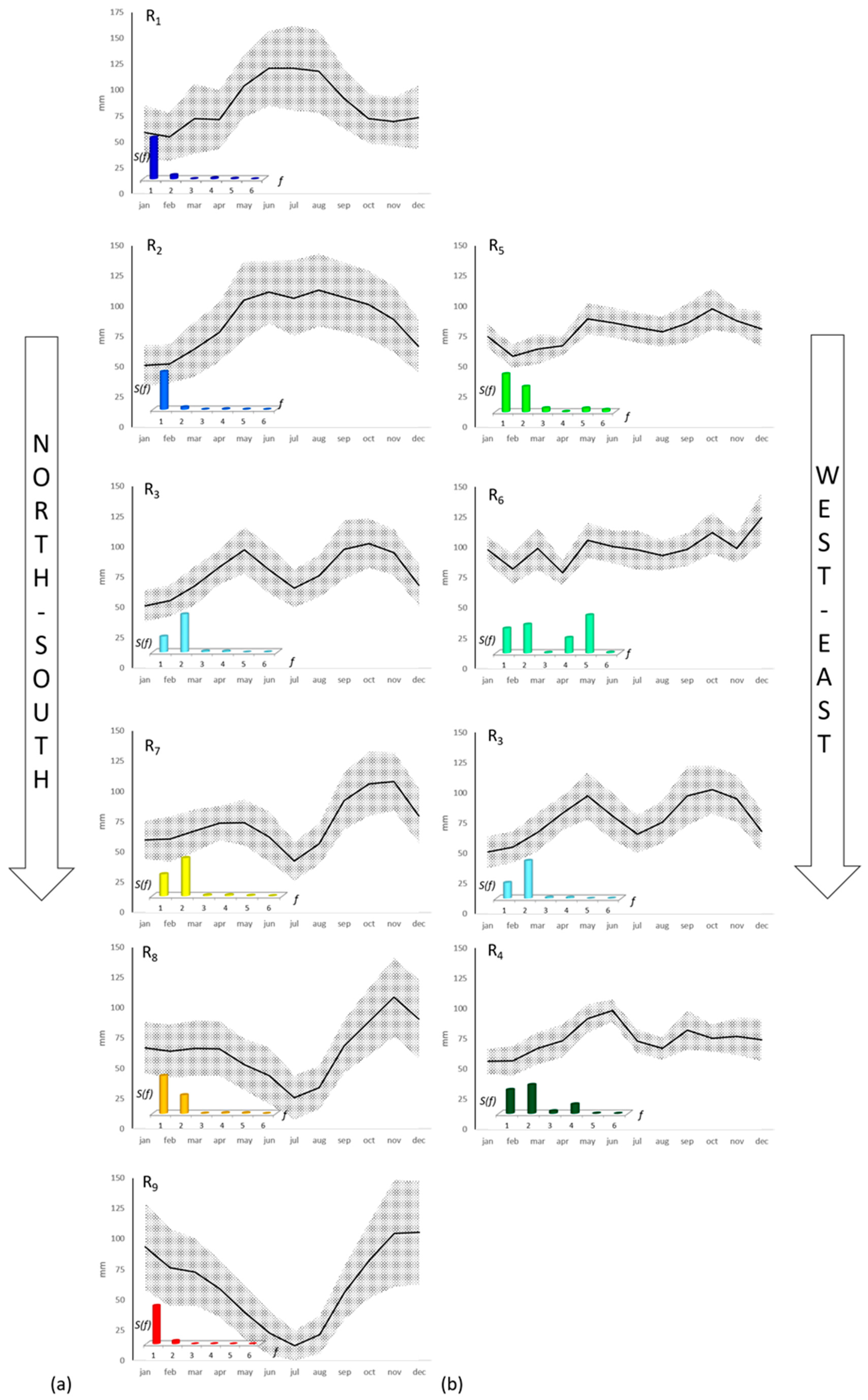
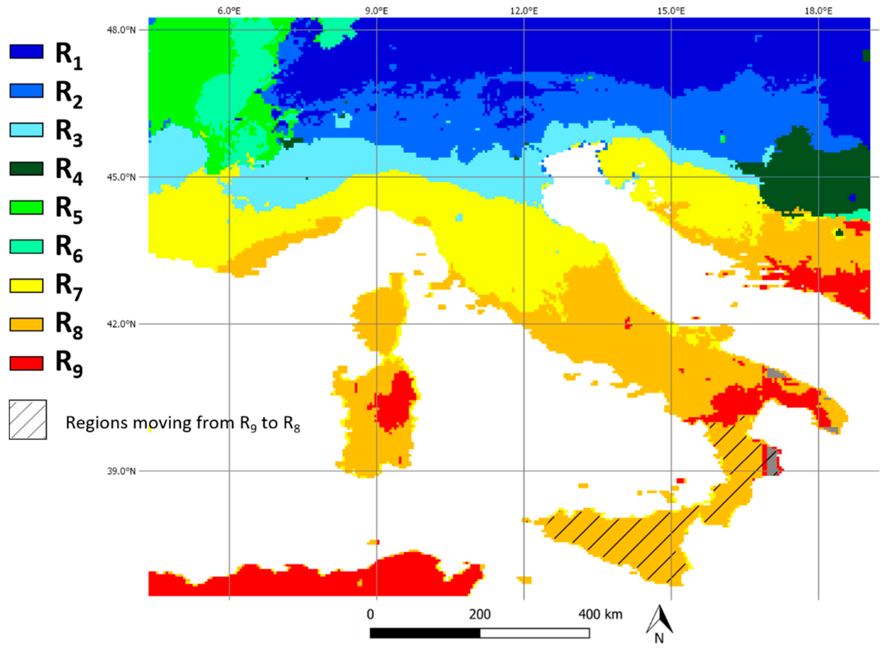
4.2. Cluster Analysis of Average Seasonal Patterns
4.3. Detection of Seasonally Asynchronous Climate Change in a Simulation-Based Scenario
5. Conclusions
Author Contributions
Funding
Acknowledgments
Conflicts of Interest
References
- Köppen, W.P. Das Geographische System der Klimate; Gebrüder Borntraeger: Berlin, Germany, 1936. [Google Scholar]
- Thornthwaite, C.W. An Approach toward a Rational Classification of Climate. Soil Sci. 1948, 66, 77. [Google Scholar] [CrossRef]
- Takemoto, K.; Kanamaru, S.; Feng, W. Climatic seasonality may affect ecological network structure: Food webs and mutualistic networks. Biosystems 2014, 121, 29–37. [Google Scholar] [CrossRef] [PubMed]
- Varpe, Ø. Life History Adaptations to Seasonality. Integr. Comp. Biol. 2017, 57, 943–960. [Google Scholar] [CrossRef] [PubMed]
- Ulijaszek, S.J.; Strickland, S.S. Seasonality and Human Ecology. Available online: https://www.beck-shop.de/ulijaszek-strickland-seasonality-human-ecology/product/630299?product=630299 (accessed on 14 May 2019).
- Senner, N.R.; Stager, M.; Cheviron, Z.A. Spatial and temporal heterogeneity in climate change limits species’ dispersal capabilities and adaptive potential. Ecography 2018, 41, 1428–1440. [Google Scholar] [CrossRef]
- Barros, V.R. Climate Change 2014—Impacts, Adaptation and Vulnerability: Part B: Regional Aspects: Volume 2, Regional Aspects: Working Group II Contribution to the IPCC Fifth Assessment Report: Amazon. It: Intergovernmental Panel on Climate Change: Libri in Altre Lingue; IPCC—Intergovernmental Panel on Climate Change/Cambridge University Press: Cambridge, UK; New York, NY, USA, 2014; p. 688. [Google Scholar]
- Mbow, H.O.P.; Reisinger, A.; Canadell, J.; O’Brien, P. Special Report on Climate Change, Desertification, Land Degradation, Sustainable Land Management, Food Security, and Greenhouse Gas Fluxes in Terrestrial Ecosystems (SRCCL)|11.06.2018|Notizia|Scienze Naturali Svizzera; IPCC—Intergovernmental Panel on Climate Change/Cambridge University Press: Cambridge, UK; New York, NY, USA, 2019; p. 32. [Google Scholar]
- Li, Q.; Lu, W.; Yang, J. A Hybrid Thresholding Algorithm for Cloud Detection on Ground-Based Color Images. J. Atmos. Ocean. Technol. 2011, 28, 1286–1296. [Google Scholar] [CrossRef]
- Bontemps, S.; Herold, M.; Kooistra, L.; Groenestijn, A.; van Hartley, A.; Arino, O.; Moreau, I.; Defourny, P. Revisiting land cover observation to address the needs of the climate modeling community. Biogeosciences 2012, 9, 2145–2157. [Google Scholar] [CrossRef]
- Coluzzi, R.; Imbrenda, V.; Lanfredi, M.; Simoniello, T. A first assessment of the Sentinel-2 Level 1-C cloud mask product to support informed surface analyses. Remote Sens. Environ. 2018, 217, 426–443. [Google Scholar] [CrossRef]
- Yang, J.; Gong, P.; Fu, R.; Zhang, M.; Chen, J.; Liang, S.; Xu, B.; Shi, J.; Dickinson, R. The role of satellite remote sensing in climate change studies. Nat. Clim. Chang. 2013, 3, 875–883. [Google Scholar] [CrossRef]
- World Meteorological Organization (WMO); United Nations Educational Scientific and Cultural Organization (UNESCO); United Nations Environment Programme (UNEP); International Council for Science (ICSU); World Meteorological Organization (WMO). GCOS, 154. Systematic Observation Requirements for Satellite-Based Products for Climate Supplemental Details to the Satellite-Based Component of the Implementation Plan for the Global Observing System for Climate in Support of the UNFCCC: 2011 Update; WMO: Geneva, Switzerland, 2011. [Google Scholar]
- Funk, C.; Peterson, P.; Landsfeld, M.; Pedreros, D.; Verdin, J.; Shukla, S.; Husak, G.; Rowland, J.; Harrison, L.; Hoell, A.; et al. The climate hazards infrared precipitation with stations—A new environmental record for monitoring extremes. Sci. Data 2015, 2. [Google Scholar] [CrossRef]
- Shukla, S.; McNally, A.; Husak, G.; Funk, C. A seasonal agricultural drought forecast system for food-insecure regions of East Africa. Hydrol. Earth Syst. Sci. 2014, 18, 3907–3921. [Google Scholar] [CrossRef]
- Beck, H.E.; Zimmermann, N.E.; McVicar, T.R.; Vergopolan, N.; Berg, A.; Wood, E.F. Present and future Köppen-Geiger climate classification maps at 1-km resolution. Sci. Data 2018, 5. [Google Scholar] [CrossRef] [PubMed]
- Mahlstein, I.; Daniel, J.S.; Solomon, S. Pace of shifts in climate regions increases with global temperature. Nat. Clim. Chang. 2013, 3, 739–743. [Google Scholar] [CrossRef]
- Zveryaev, I.I. Seasonality in precipitation variability over Europe. J. Geophys. Res. 2004, 109. [Google Scholar] [CrossRef]
- Weiss, M.; Banko, G. Ecosystem Type Map v3.1–Terrestrial and Marine Ecosystems; European Environment Agency (EEA)—European Topic Centre on Biological Diversity; ETC/BD: Paris, France, 2018; p. 79. [Google Scholar]
- Lanfredi, M.; Coppola, R.; D’Emilio, M.; Imbrenda, V.; Macchiato, M.; Simoniello, T. A geostatistics-assisted approach to the deterministic approximation of climate data. Environ. Modell. Softw. 2015, 66, 69–77. [Google Scholar] [CrossRef]
- Kotzeva, M. Eurostat Regional Yearbook-2018 Edition; General and Regional Statistics; Publications Office of the European Union: Brussels, Belgium, 2018; ISBN 978-92-79-87878. [Google Scholar]
- Imbrenda, V.; Coluzzi, R.; Lanfredi, M.; Loperte, A.; Satriani, A.; Simoniello, T. Analysis of landscape evolution in a vulnerable coastal area under natural and human pressure. Geomat. Nat. Hazards Risk 2018, 9, 1249–1279. [Google Scholar] [CrossRef]
- Lanfredi, M.; Coppola, R.; Simoniello, T.; Coluzzi, R.; D’Emilio, M.; Imbrenda, V.; Macchiato, M. Early Identification of Land Degradation Hotspots in Complex Bio-Geographic Regions. Remote Sens. 2015, 7, 8154–8179. [Google Scholar] [CrossRef]
- Imbrenda, V.; D’emilio, M.; Lanfredi, M.; Macchiato, M.; Ragosta, M.; Simoniello, T. Indicators for the estimation of vulnerability to land degradation derived from soil compaction and vegetation cover. Eur. J. Soil Sci. 2014, 65, 907–923. [Google Scholar] [CrossRef]
- Caloiero, T.; Veltri, S.; Caloiero, P.; Frustaci, F. Drought Analysis in Europe and in the Mediterranean Basin Using the Standardized Precipitation Index. Water 2018, 10, 1043. [Google Scholar] [CrossRef]
- Greco, S.; Infusino, M.; De Donato, C.; Coluzzi, R.; Imbrenda, V.; Lanfredi, M.; Simoniello, T.; Scalercio, S. Late Spring Frost in Mediterranean Beech Forests: Extended Crown Dieback and Short-Term Effects on Moth Communities. Forests 2018, 9, 388. [Google Scholar] [CrossRef]
- Hanel, M.; Rakovec, O.; Markonis, Y.; Máca, P.; Samaniego, L.; Kyselý, J.; Kumar, R. Revisiting the recent European droughts from a long-term perspective. Sci. Rep. 2018, 8, 9499. [Google Scholar] [CrossRef]
- Hoerling, M.; Eischeid, J.; Perlwitz, J.; Quan, X.; Zhang, T.; Pegion, P. On the Increased Frequency of Mediterranean Drought. J. Clim. 2011, 25, 2146–2161. [Google Scholar] [CrossRef]
- Nolè, A.; Rita, A.; Ferrara, A.M.S.; Borghetti, M. Effects of a large-scale late spring frost on a beech (Fagus sylvatica L.) dominated Mediterranean mountain forest derived from the spatio-temporal variations of NDVI. Ann. For. Sci. 2018, 75, 83. [Google Scholar] [CrossRef]
- Spinoni, J.; Naumann, G.; Vogt, J.; Barbosa, P. Meteorological Droughts in Europe: Events and Impacts: Past Trends and Future Projections; Publications Office of the European Union: Luxembourg, 2016; p. 134. [Google Scholar]
- Cassardo, C.; Loglisci, N.; Paesano, G.; Rabuffetti, D.; Qian, M.W. The Hydrological Balance of the October 2000 Flood in Piedmont, Italy: Quantitative Analysis and Simulation. Phys. Geogr. 2006, 27, 411–434. [Google Scholar] [CrossRef]
- Duclos, P.; Vidonne, O.; Beuf, P.; Perray, P.; Stoebner, A. Flash flood disaster-nîmes, France, 1988. Eur. J. Epidemiol. 1991, 7, 365–371. [Google Scholar] [CrossRef]
- Grieser, J.; Beck, C.; Rudolf, B. The Summer Flooding 2005 in Southern Bavaria—A Climatological Review; Selbstverlag: Offenbach am Main, Germany, 2006; pp. 168–173. [Google Scholar]
- Massari, C.; Camici, S.; Ciabatta, L.; Brocca, L. Exploiting Satellite-Based Surface Soil Moisture for Flood Forecasting in the Mediterranean Area: State Update versus Rainfall Correction. Remote Sens. 2018, 10, 292. [Google Scholar] [CrossRef]
- Peruccacci, S.; Brunetti, M.T.; Gariano, S.L.; Melillo, M.; Rossi, M.; Guzzetti, F. Rainfall thresholds for possible landslide occurrence in Italy. Geomorphology 2017, 290, 39–57. [Google Scholar] [CrossRef]
- Rickenmann, D.; Badoux, A.; Hunzinger, L. Significance of sediment transport processes during piedmont floods: The 2005 flood events in Switzerland. Earth Surf. Processes Landf. 2016, 41, 224–230. [Google Scholar] [CrossRef]
- Saunders, M.A. Central and Eastern European Floods of July 1997; Benfield Greig Hazard Research Centre: London, UK, 1998. [Google Scholar]
- Silvestro, F.; Gabellani, S.; Giannoni, F.; Parodi, A.; Rebora, N.; Rudari, R.; Siccardi, F. A hydrological analysis of the 4 November 2011 event in Genoa. Nat. Hazards Earth Syst. Sci. 2012, 12, 2743–2752. [Google Scholar] [CrossRef]
- Janowiak, J.E.; Joyce, R.J.; Yarosh, Y. A Real-Time Global Half-Hourly Pixel-Resolution Infrared Dataset and Its Applications. Bull. Am. Meteorol. Soc. 2001, 82, 205–218. [Google Scholar] [CrossRef]
- Knapp, K.R.; Ansari, S.; Bain, C.L.; Bourassa, M.A.; Dickinson, M.J.; Funk, C.; Helms, C.N.; Hennon, C.C.; Holmes, C.D.; Huffman, G.J.; et al. Globally Gridded Satellite Observations for Climate Studies. Bull. Am. Meteorol. Soc. 2011, 92, 893–907. [Google Scholar] [CrossRef]
- Huffman, G.J.; Bolvin, D.T.; Nelkin, E.J.; Wolff, D.B.; Adler, R.F.; Gu, G.; Hong, Y.; Bowman, K.P.; Stocker, E.F. The TRMM Multisatellite Precipitation Analysis (TMPA): Quasi-Global, Multiyear, Combined-Sensor Precipitation Estimates at Fine Scales. J. Hydrometeorol. 2007, 8, 38–55. [Google Scholar] [CrossRef]
- Huffman, G.J.; Adler, R.F.; Bolvin, D.T.; Nelkin, E.J. The TRMM Multi-Satellite Precipitation Analysis (TMPA). In Satellite Rainfall Applications for Surface Hydrology; Gebremichael, M., Hossain, F., Eds.; Springer: Dordrecht, The Netherlands, 2010; pp. 3–22. ISBN 978-90-481-2915-7. [Google Scholar]
- Saha, S.; Moorthi, S.; Pan, H.-L.; Wu, X.; Wang, J.; Nadiga, S.; Tripp, P.; Kistler, R.; Woollen, J.; Behringer, D.; et al. NCEP Climate Forecast System Version 2 (CFSv2) 6-Hourly Products; National Center for Atmospheric Research: Boulder, CO, USA, 2011; pp. 1015–1058. [Google Scholar]
- Saha, S.; Moorthi, S.; Pan, H.-L.; Wu, X.; Wang, J.; Nadiga, S.; Tripp, P.; Kistler, R.; Woollen, J.; Behringer, D.; et al. The NCEP Climate Forecast System Reanalysis. Bull. Am. Meteorol. Soc. 2010, 91, 1015–1058. [Google Scholar] [CrossRef]
- Mac Queen, J. Some Methods for Classification and Analysis of Multivariate Observations; University of California: Berkeley, CA, USA, 1967; Volume 1, pp. 281–297. [Google Scholar]
- Rousseeuw, P.J. Silhouettes: A graphical aid to the interpretation and validation of cluster analysis. J. Comput. Appl. Math. 1987, 20, 53–65. [Google Scholar] [CrossRef]
- Jenkins, G.M.; Watts, D.G. Spectral Analysis and Its Applications; Holden-Day Series in Time Series Analysis; Holden-Day: London, UK, 1969. [Google Scholar]
- Kovats, R.S.; Valentini, R.; Bouwer, L.M.; Georgopoulou, E.; Jacob, D.; Martin, E.; Rounsevell, M.; Soussana, J.F. Climate Change 2014—Impacts, Adaptation and Vulnerability: Part B: Regional Aspects: Volume 2, Regional Aspects: Working Group II Contribution to the IPCC Fifth Assessment Report: Amazon.it; Intergovernmental Panel on Climate Change: Cambridge, UK; New York, NY, USA, 2014; pp. 1267–1326. [Google Scholar]
- Kjellström, E.; Nikulin, G.; Hansson, U.; Strandberg, G.; Ullerstig, A. 21st century changes in the European climate: Uncertainties derived from an ensemble of regional climate model simulations. Tellus A 2011, 63, 24–40. [Google Scholar] [CrossRef]


| Cluster | Number of Pixels |
|---|---|
| C1 | 1713 |
| C2 | 4862 |
| C3 | 6828 |
| C4 | 9854 |
| C5 | 8681 |
| C6 | 5532 |
| Region | Number of Pixels |
|---|---|
| R1 | 7031 |
| R2 | 5090 |
| R3 | 3266 |
| R4 | 1332 |
| R5 | 1833 |
| R6 | 1216 |
| R7 | 6000 |
| R8 | 6492 |
| R9 | 5210 |
© 2020 by the authors. Licensee MDPI, Basel, Switzerland. This article is an open access article distributed under the terms and conditions of the Creative Commons Attribution (CC BY) license (http://creativecommons.org/licenses/by/4.0/).
Share and Cite
Lanfredi, M.; Coluzzi, R.; Imbrenda, V.; Macchiato, M.; Simoniello, T. Analyzing Space–Time Coherence in Precipitation Seasonality across Different European Climates. Remote Sens. 2020, 12, 171. https://doi.org/10.3390/rs12010171
Lanfredi M, Coluzzi R, Imbrenda V, Macchiato M, Simoniello T. Analyzing Space–Time Coherence in Precipitation Seasonality across Different European Climates. Remote Sensing. 2020; 12(1):171. https://doi.org/10.3390/rs12010171
Chicago/Turabian StyleLanfredi, Maria, Rosa Coluzzi, Vito Imbrenda, Maria Macchiato, and Tiziana Simoniello. 2020. "Analyzing Space–Time Coherence in Precipitation Seasonality across Different European Climates" Remote Sensing 12, no. 1: 171. https://doi.org/10.3390/rs12010171
APA StyleLanfredi, M., Coluzzi, R., Imbrenda, V., Macchiato, M., & Simoniello, T. (2020). Analyzing Space–Time Coherence in Precipitation Seasonality across Different European Climates. Remote Sensing, 12(1), 171. https://doi.org/10.3390/rs12010171