Abstract
A regional zenith tropospheric delay (ZTD) empirical model, referred to as SHAtropE (SHanghai Astronomical observatory tropospheric delay model—Extended), is developed and provides tropospheric propagation delay corrections for users in China and the surrounding areas with improved accuracy. The SHAtropE model was developed based on the ZTD time series of the continuous GNSS sites from the Crustal Movement Observation Network of China (CMONOC) and GNSS sites of surrounding areas. It combines the exponential and periodical functions and is provided as regional grids with a resolution of 2.5° × 2.0° in longitude and latitude. At each grid point, the exponential function converts the ZTD from the site height to the ellipsoid, and the periodical terms, including both annual and semi-annual periods, describe ZTD’s temporal variation. Moreover, SHAtropE also provides the predicted ZTD uncertainty, which is valuable in Precise Point Positioning (PPP) with ZTD being constrained for faster convergence. The data of 310 GNSS sites over 7 years were used to validate the new model. Results show that the SHAtropE ZTD has an accuracy of 3.5 cm in root mean square (RMS) quantity, which has a mean improvement of 35.2% and 5.4% over the UNB3m (5.4 cm) and GPT3 (3.7 cm) models, respectively. The predicted uncertainty of SHAtropE ZTD shows seasonal variations, where the values are larger in summer than in winter. By applying the SHAtropE model in the static PPP, the convergence time of GPS-only and BDS-only solutions are reduced by 8.1% and 14.5% respectively compared to the UNB3m model, and the reductions are 6.9% and 11.2% respectively for the GPT3 model. As no meteorological data are required for the implementation of the model, the SHAtropE could thus be a refined tropospheric model for GNSS users in mainland China and the surrounding areas. The method of modeling the ZTD uncertainty can also be used in further global tropospheric delay modeling.
1. Introduction
Through the path that radio signals traverse the troposphere, the signals are delayed to a magnitude of meters with respect to free-space propagation [1]. This delay, referred to as tropospheric delay, is a function of the tropospheric refractive index, and is dependent on the local temperature, pressure, and relative humidity. Tropospheric delay is one of the main error sources in space geodesy techniques, i.e., Global Navigation Satellite System (GNSS), Very Long Baseline Interferometry [2], satellite altimetry [3,4], etc. Tropospheric delay is usually modeled as the sum of a hydrostatic and a non-hydrostatic (wet) part, where the hydrostatic delay (referred as ZHD at zenith) accounts for 90% of the zenith total delay (ZTD), while the wet delays (referred as ZWD at zenith) contributes to the precipitable water vapor are hard to model since the water vapor varies a lot [5]. Consequently, wet delays are usually estimated as unknown parameters in GNSS data analysis. On the other hand, using the precise a priori tropospheric delay in GNSS data processing with proper constraint can improve the convergence time and the short-term precision [6,7,8,9,10,11].
The discrete tropospheric delays can be derived from radiosonde observations and Numerical Weather Model (NWM), e.g., European Centre for Medium-Range Weather Forecasts (ECMWF). The latter one has a global coverage and a ZTD accuracy of 1–2 cm can be achieved [12,13]. On the other hand, the empirical tropospheric delay models are widely used, as they provide real-time data and do not need any external information. The empirical models could be determined using discrete ZTD data from radiosonde, NWM, and GNSS products. The radiosonde observations are used for the early-stage models, e.g., the Hopfield model [14], the Saastamoinen [15], the UNB series models (UNB1 through UNB4) [16,17] and EGNOS model [18], etc. The Global Pressure and Temperature (GPT) [19,20] model is determined using the ECMWF, and provides the pressure and temperature at any location of the earth surface using the spherical harmonic function. The improved version of GPT, i.e., GPT2 [21], GPT2w [22], and GPT3 [23], all use a global grid with better accuracy and more tropospheric information. All these models determine the global meteorological parameters, e.g., pressure, temperature, water vapor, and then they are used as inputs of other models, e.g., the Saasamoinen and the Askne and Nordius [24] models to calculate tropospheric delays. Recently, some new models have provided tropospheric delay directly, such as the IGGtrop [25,26] and GZTD [27,28], where the ZTD time series from NWM are directly modeled. It has been demonstrated that by appropriately constraining the tropospheric parameter using the empirical models, the PPP convergence time could be accelerated [7,9].
With the expanding of GNSS ground tracking network, precise ZTD products have been derived with improved temporal and spatial resolutions. Covering the whole area of mainland China, the GNSS network of the Crustal Movement Observation Network of China (CMONOC) consists of around 260 well-distributed continuous sites. The GNSS analysis center at Shanghai Astronomical Observatory (abbreviated as SHA, [29]) has been providing the precise ZTD time series since 2011. By using the precise ZTD products of SHA in mainland China and the precise ZTD products of surrounding GNSS sites from the Nevada Geodetic Laboratory [30], we develop a regional tropospheric delay empirical model, namely SHAtropE (SHanghai Astronomical observatory tropospheric delay model—Extended), for China and surrounding areas. More importantly, for the first time we provide the a priori predicted uncertainty of the empirical ZTD at any time and any location, which can be used as a priori constraint in GNSS PPP to accelerate its convergence. The accuracy of other empirical models is available in several studies about the model assessment, but none of these models provide the epoch-wise location-specified ZTD uncertainty, which is achieved in this study.
This paper presents the details of the empirical SHAtropE ZTD model and its application in the PPP. Section 2 introduces the input ZTD data, where 7 years of data from January 2012 to December 2018 of 310 sites are used and their spatial and temporal characteristics are analyzed. Section 3 describes the method for the determination of SHAtropE model. Section 4 validates the SHAtropE model, where ZTD values of the 6 years are used for inner-consistency validation and the ZTDs in the year of 2018 are used for the validation of the predicted period [31], and one-month data are used for PPP assessment. Section 5 summaries the main conclusions.
2. Input Data
The CMONOC GNSS network starts full operation since 2011, and the SHA GNSS Analysis Center includes this regional network into its routine global GNSS network data analysis [29,32], providing site-wise ZTD products together with other precise products, e.g., site coordinates, satellite orbits and clocks, etc. The left panel in Figure 1 shows the distribution of these sites, including 223 sites from CMONOC and 87 sites from the local GNSS networks and IGS (http://www.igs.org/network). The sites have a good coverage over this region except for the Tibetan Plateau. The precise ZTD estimates from January 2012 to December 2018 of all CMONOC GNSS sites and other surrounding GNSS sites are used, where data of the first 6 years are used for the SHAtropE model determination and the data of the whole 7 years are used for the model assessment. The right panel in Figure 1 shows the ZTD usable days at each site during January 2012–December 2017, of which most sites have a period of valid data of more than 1500 days, and a minimum time of more than 2 years.
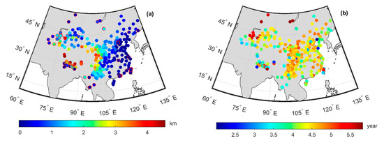
Figure 1.
(a) Distribution of sites used and (b) the valid days of each site. The non-Crustal Movement Observation Network of China (CMONOC) site in panel (a) are marked with red edge, the color bar in (a) shows the site height in km.
The SHA GNSS analysis center follows the IGS data analysis strategies using a zero-difference approach based on 5-min sampling data of selected global GNSS network [29,32]. SHA provides a precise ZTD product with a resolution of 1 h. The ZTD product has an agreement of around 4 mm compared to the IGS ZTD products [33], thus it is reliable to be used in the empirical ZTD modeling. The ZTD products of the Non-CMONOC sites are from the Nevada Geodetic Laboratory (NGL, http://geodesy.unr.edu/). For details regarding these sites we refer to Blewitt et al. [30]. All precise ZTD products from SHA and NGL are referred to as RAW ZTD in the following text.
Temporal Variation of RAW ZTD Time Series
The ZTD of a specific site at a specific day could be expressed as the combination of an empirical model and the residuals at this day [34]:
where is the RAW ZTD, is the modeled ZTD and is the fitting residual; is the average annual ZTD; A1 and d1 are the amplitude and initial phase of the annual component; A2 and d2 are the amplitude and the initial phase of the semi-annual component.
The residual cannot be precisely modeled due to the high variable water vapor component and the atmosphere pressure fluctuation. It is for this reason that the empirical tropospheric delay suffers from accuracy loss. The residual variation, however, is highly related to the weather condition, e.g., the fluctuation in summer is much larger than that in winter, thus, the empirical model suffers a larger error in summer than in winter. The absolute value of the residuals can be modeled as:
where is the absolute value of the RAW ZTD residuals, is the modeled absolute value of the ZTD residuals and is the fitting residual; B0 is the average annual absolute value of empirical ZTD residual; B1 and f1 are the amplitude and initial phase of annual component; B2 and f2 are amplitude and initial phase of semi-annual component. By definition, the term presents the uncertainty of the above-defined empirical tropospheric delay, and it can be used to predict the uncertainty of the empirical model, thus provides better a priori constraint of troposphere delays when applying the model in positioning.
Using 6 years of data, we first derive the empirical temporal ZTD variations model for each site. Figure 2 shows the model parameters and the fitting RMS of each site according to their geographical distribution. The fitting RMS values (panel (a)) show large differences among regions, where the largest RMS value is 7 cm and the smallest one is 1 cm. The fitting errors are generally smaller in western parts of the studied area and larger in east parts, where the content of water vapor and its variation is much larger. For the fitted parameters, each parameter shows spatial similarity, where the parameters are quite close for nearby sites. The spatial variation of the constant term A0 (panel (b)) for all sites is from 1.4 to 2.5 m, where nearby sites show large similarity, and a rough linear regression between the value and the site height could be observed. The annual amplitude A1 (panel (c)) ranges from −2 to −14 cm, where the maximum (absolute value) is in the vicinity of (25°N, 80°E) and the minimum is near (40°N, 65°E). The semi-annual amplitude A2 (panel (e)) ranges from 1 to −5 cm, where the maximum is in the vicinity of (25°N, 80°E).
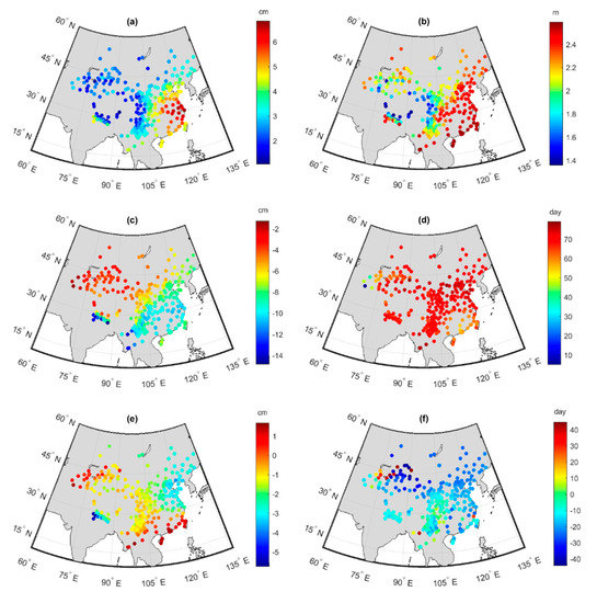
Figure 2.
Parameters of the empirical temporal zenith tropospheric delay (ZTD) variations model of each site. (a) fitting root mean square (RMS); (b) the constant term A0; (c) annual amplitude A1; (d) initial phase of annual term d1; (e) semi-annual amplitude A2; (f) initial phase of semi-annual term d2. It should be noted that the amplitudes are modified to make the phase terms continuous and in the range of (0, 90) and (−45, 45) for the annual and semi-annual terms, respectively.
The fitted parameters of the absolute ZTD residuals using Equation (2) are presented in Figure 3. The annual average value of the absolute biases B0 (panel (b)) ranges from 1 to 6 cm, and the maximum value is in the vicinity of (30°N, 120°E). This is consistent with Figure 2a, where the largest value of fit RMS is in the same area. The annual amplitude B1 (panel (c)) could be as large as 2 cm, while the semi-annual amplitude B2 (panel (e)) could be as large as 1.5 cm. The initial phases of annual and semi-annual terms (panel (d) and (f)) both show a similar pattern for nearby sites.
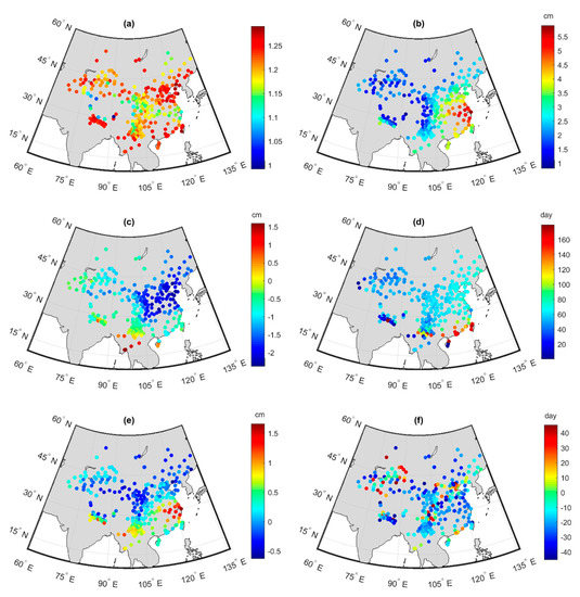
Figure 3.
The fit parameters of the absolute ZTD fit residuals. (a) the ratio between the RMS of RAW ZTD fit residuals and the RMS of modeled residuals; (b) the constant term B0; (c) annual amplitude B1; (d) initial phase of annual term f1; (e) semi-annual amplitude B2; (f) initial phase of semi-annual term f2.
It should be noted that the RAW and modeled ZTD residuals, i.e., and are different in terms of RMS statistics. The ratio between the RMS of RAW ZTD fit residuals and the RMS of modeled residuals could be defined as: , which is shown in Figure 3a. The modeling of residuals introduces a down-scale of the RMS statistics in a magnitude of about 1.2, showing the modeled residuals account for about 80% of the real residuals. Thus, to keep the consistency of modeled residuals and the RAW residuals, this ratio value is used for further model determination.
3. Model Determination of SHAtropE
It is widely acknowledged that ZTD is highly correlated with site height; thus, it should be carefully considered in the empirical ZTD model determination. There are two main approaches to account for the influence of the height difference on ZTD modeling. The first is to set up fitting models with site heights as input [26], and the other one is to correct the ZTD difference according to the site height difference with respect to a reference surface [35]. In the modeling of the SHAtropE, we choose the ellipsoid as the reference plane and the empirical temporal ZTD variations model of all sites are covert to this plane. The convert model functional parameters of each site are then interpolated to derive the functional parameters at pre-defined grids.
3.1. ZTD with the Ellipsoid as Reference Surface
Considering the site height shown in Figure 1a and the constant term A0 in Figure 2b, the annual average ZTD is reversely proportional to site height. Figure 4 shows the relation of the annual average ZTD and ellipsoidal height of each site, where sites are separated into five groups according to site latitudes and each group is represented by different color, and all the sites are defined as the sixth group. For each group, the relation between annual average ZTD at the site ellipsoidal height (), and the annual average ZTD on the ellipsoid surface (), can be expressed as an exponential formula [36]:
where is Euler’s number, is the tropospheric scale height.
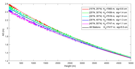
Figure 4.
Annual average ZTD w.r.t. site ellipsoidal height and the exponential fitting curves. The scaled height and the fit RMS are also presented in the figure.
The fitted exponential curves for each group are shown in Figure 4, where the tropospheric scale height for each group is also presented (as in Table 1). As shown in Figure 4, the RMS values of fit residuals are (0.6, 1.4, 1.6, 1.3, 1.1, 5.5) cm for the six groups, respectively. The fit RMS value (5.5 cm) of all the sites together is much larger than that of all other five separated groups. Therefore, by dividing the sites into different groups according to the latitude, the fitting result shows a significant improvement.

Table 1.
The fitted tropospheric scale height for different latitude groups.
3.2. ZTD Temporal Variations on the Ellipsoid
Equation (3) coverts the ZTD from site ellipsoidal height to the ellipsoid, and the ZTD variation due to the site height differences is thus removed. Combining Equations (1) and (3), the empirical ZTD model for each site can thus be written as:
where A0,e, A1,e and A2,e are the mean ZTD, ZTD annual amplitude and ZTD semi-annual amplitude of the site on ellipsoid. With the tropospheric scale height from Table 1 (also Figure 4), A0,e, A1,e, and A2,e can be directly calculated using the fitted parameters A0, A1, and A2 in Section 2, through the following equations:
The parameters of A0,e, A1,e, and A2,e of all the sites are plotted in Figure 5. The spatial variation of the term A0,e (panel (a)) for all sites is from 2.4 to 2.6 m, where its variation range is much smaller than that of A0 in Figure 2. The annual amplitude A1,e (panel (b)) ranges from 2 to 14 cm, and the semi-annual amplitude A2,e ranges from 1 to 5 cm (panel (c)).
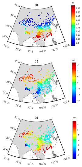
Figure 5.
(a) The constant term A0,e, (b) the annual amplitude term A1,e, and (c) the semi-annual term A2,e of ZTD scaled on the ellipsoid of each site.
3.3. Gridded ZTD Modeling of SHAtropE
As shown in the previous section, the parameters of empirical temporal ZTD variations model are rather close for nearby sites. Thus, we set up a spatial-correlated grid model, i.e., SHAtropE, for the study areas. The modeling steps are as follows:
- For each site, RAW ZTD from SHA (CMONOC sites) and NGL (Non-COMONC sites) are used to derive the five functional parameters A0, A1, d1, A2, d2 and the five ZTD uncertainty functional parameters B0, B1, f1, B2, f2, based on Equations (1) and (2), respectively.
- For each site, the five ZTD functional parameters of empirical model are converted to the ellipsoid using the exponential function and the constants in in Table 1, and the related parameters on the ellipsoid, i.e., A0,e, A1,e, and A2,e are derived.
- Divide the study areas [70°E–135°E, 18°N–54°N] as grids with a resolution of 2.5° and 2.0° on longitude and latitude, respectively. The 5 ZTD functional parameters on the ellipsoid of each grid point is derived by the inverse distance weighted (IDW) function [37] using the parameters of nearby sites. And the ZTD uncertainty functional parameters B0, B1, f1, B2, f2 for each grid could also be derived by the IDW approach.
The exponential constants of latitude groups, the ten ZTD/uncertainty functional parameters of each grid point are the basic components of the SHAtropE. The characteristics of the data sets used in this study are summarized in Table 2.
Table 2.
Characteristics of the data used in this study.
4. Assessment of SHAtropE
SHAtropE provides users with ten ZTD/uncertainty functional parameters of each grid point in an ASCII-file (30 KB with the resolution of 2.5° (Longitude) × 2.0° (Latitude). On the user side, the calculation of the ZTD and its uncertainty using the SHAtropE model requires the input of site location (longitude, latitude, ellipsoidal height) and the day of the year. In the first step, the user calculates the five ZTD functional parameters (A0,e, A1,e, d1, A2,e, and d2) and uncertainty functional parameters (B0, B1, f1, B2, f2) at its location using the nearby grid points with the bilinear interpolation scheme. Then the ZTD at the user location is calculated according to Equation (4) in the second step. As for the uncertainty of SHAtropE ZTD, user first calculate the modeled value according to Equation (2), and this value is multiplied by 1.2 to derive the uncertainty value.
In the following, we use three methods to assess the performance of the SHAtropE model. The ZTD from SHAtropE model is called SHAtropE ZTD in the following text. Three methods are: (1) Comparisons between SHAtropE ZTD and RAW ZTD using data from January 2012 to December 2017 of all the used sites. This comparison shows inner-accuracy, as the ZTDs of each site during this period are used for the SHAtropE modeling. (2) Comparisons between SHAtropE ZTD and RAW ZTD using the whole year (2018) data of all sites. This comparison shows external-accuracy, because the predicted SHAtropE ZTD values are used and validated. (3) Precise Point Positioning using SHAtropE ZTD as the a priori input, where the ZTD is constrained using the predicted uncertainty of the model.
4.1. ZTD Accuracy of SHAtropE
For the ZTD comparisons, RAW ZTD is chosen as reference and the mean bias and RMS are calculated as follows:
where and are RAW ZTD and SHAtropE ZTD.
For comparison, the other two widely used models, e.g., UNB3m and GPT3, are also evaluated using the RAW ZTD products. UNB3m is a representative model based on radiosonde observations, and it uses a lookup table, where the different parameters are divided by latitude. GPT3 is the latest version of the tropospheric delay models developed by TU Wien. It is based on the numerical weather model, and the product is provided with a global grid. GPT3 model has two available resolutions, i.e., 1° × 1° and 5° × 5°. In this study the 1° × 1° grid product is used, as it has a better accuracy than the other one.
Figure 6 shows the RAW ZTD, SHAtropE ZTD and its uncertainty, and the differences between RAW/SHAtropE ZTD from January 2012 to December 2018 for sites NMER (at north-east China with low site altitude) and YNLJ (at south-west China with high site altitude). The RMS values of the ZTD differences between RAW ZTD and SHAtropE ZTD are 2.0 cm and 1.9 cm for the two sites, and that of the predicted uncertainty of SHAtropE (black line) are 1.8 cm and 2.1 cm, indicating a good agreement of the predicted uncertainty. Relative larger variations are observed in summer seasons for both sites. For site NMER with lower ellipsoidal height, the ZTD variation in summer season is so big that the residuals may even beyond ±2 times of the predicted uncertainty; while for site YNLJ with higher ellipsoidal height, the ZTD variation is almost all within ±1 times of the predicted uncertainty. As for the modeled uncertainty, apparent seasonal variation is observed. Comparing the results of the modeling and prediction periods, i.e., the 2012–2017 and 2018, respectively, no apparent divergence is observed, showing that SHAtropE is very reliable in both predicted ZTD and its uncertainty values.
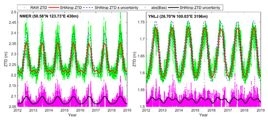
Figure 6.
RAW ZTD (green) and SHAtropE ZTD (red) for two sites: NMER (left) and YNLJ (right). The absolute value (magenta) of the differences between RAW ZTD and SHAtropE, and the predicted uncertainty provided by SHAtropE (black) are presented with an offset (2.05 m at NMER and 1.50 m at YNLJ) for better visualization.
Figure 7 shows the RMS and BIAS of the whole period from January 2012 to December 2018 for all sites. For comparisons, the same ZTD quantities are derived for UNB3m/GPT3 models. As shown in Figure 7 that SHAtropE has no significant bias for all sites, with the maximum bias of 2.9 mm and minimum one of −3.2 mm. It achieves the best accuracy with the RMS less than 3.5 cm for all sites, and the maximum RMS appears in the vicinity of (30°N, 120°E). UNB3m shows the worst accuracy with mean RMS of 5.4 cm, and the BIAS and RMS are apparently separated into two groups, where sites in lower latitude have much worse performance than those in higher latitude. GPT3 has a similar performance compared to SHAtropE, with a slightly larger RMS value of 3.7 cm.
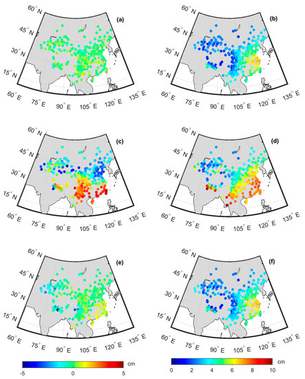
Figure 7.
Comparisons between RAW ZTD and empirical models during the period of 2012–2018. Left: mean value of ZTD biases for (a) SHAtropE, (c) UNB3m, and (e) GPT3; Right: RMS values of the ZTD biases for (b) SHAtropE, (d) UNB3m, and (f) GPT3.
Figure 8 shows the mean BIAS and RMS of all sites, arranged into the 2012–2017 and 2018 groups, where the first group represents the inner-accuracy and the latter for external-accuracy. For the mean BIAS, SHAtropE is of (0.0, 0.2) cm for inner-accuracy and external-accuracy, while they are of (0.4, 0.5) cm and (−0.2, 0.1) cm for UNB3m and GPT3, respectively. For the RMS, they are of (3.5, 3.6) cm, (5.4, 5.6) cm, and (3.7, 3.8) cm for SHAtropE, UNB3m and GPT3, respectively.
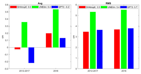
Figure 8.
Mean values (left panel) and RMS values (right panel) of the ZTD bias for the three different models: SHAtropE (red), UNB3m (green), and GPT3 (blue). The statistics of two periods: 2012–2017 and 2018 are presented separately, and the value of the whole period is presented in the legend.
4.2. The Predicted ZTD Uncertainty of SHAtropE
Unlike other empirical ZTD models, for the first time SHAtropE provides not only the ZTD model but also the ZTD uncertainty. In this section we evaluate the predicted ZTD uncertainty of SHAtropE by comparing it to the RMS statistics of the differences between SHAtropE ZTD and RAW ZTD.
As shown in Figure 6, the predicted SHAtropE ZTD uncertainty is time variable. Figure 9 shows the predicted uncertainty of SHAtropE ZTD (in left panels) and the differences between the uncertainty and the RMS value of ZTD biases (the value is Section 4.1). The left subplots of Figure 9 show the seasonal mean uncertainty quantities, where four seasons are defined according to activities of the ZTD variation. The predicted ZTD uncertainty of SHAtropE shows clear seasonal variation, where the largest values are demonstrated in Jun-Jul-Aug, especially for sites with longitude greater than 105°E, while it is less than 2 cm in the season of Dec-Jan-Feb for most sites. The right panels in Figure 9 show the differences between the predicted ZTD uncertainty and the actual RMS of SHAtropE (shown in Figure 7). In general, the predicted ZTD uncertainty of SHAtropE has a good agreement with the RMS value of SHAtropE ZTD, with mean difference of less than 5 mm, and they show no seasonal variation for all sites.
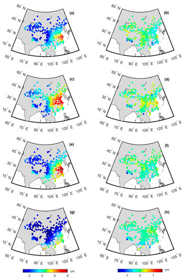
Figure 9.
Left: predicted ZTD uncertainty of SHAtropE during the period of 2012–2018 in different seasons: (a) Mar-Apr-May, (c) Jun-Jul-Aug, (e) Sep-Oct-Nov, and (g) Dec-Jan-Feb; Right: the difference between predicted uncertainty of SHAtropE and the RMS value of SHAtropE ZTD w.r.t. RAW ZTD during the period of 2012–2018 for different seasons: (b) Mar-Apr-May, (d) Jun-Jul-Aug, (f) Sep-Oct-Nov, and (h) Dec-Jan-Feb.
Figure 10 shows the statistics of the RMS and predicted uncertainty of SHAtropE of all sites during different seasons, separating into the 2012–2017 and 2018 groups. Again, the statistics show the overall divergence of these two quantities is less than 2 mm for both modeling and prediction.
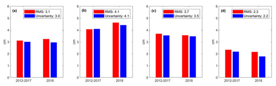
Figure 10.
RMS statistics of the SHAtropE ZTD RMS w.r.t. RAW ZTD, and the predicted ZTD uncertainty of the model during 2012–2017 (red) and 2018 (blue) in different seasons: (a) Mar-Apr-May, (b) Jun-Jul-Aug, (c) Sep-Oct-Nov, and (d) Dec-Jan-Feb. The average values of the whole period 2012-2018 are presented in the legend.
4.3. Precise Point Positioning Performance Improvement Using SHAtropE Model
To evaluate the effect of three types of tropospheric model (SHAtropE, UNB3m and GPT3) on the GNSS PPP performances, GPS and BDS observation datasets collected from 29 CMONOC sites for 1–28 February 2019 (DoY from 32 to 59) are selected and utilized for statistical analysis. All CMONOC sites are equipped with Trimble NetR9 receivers. Details of the models and strategies related to data processing for GPS/BDS static PPP are shown in Table 3. For the assessment of the PPP solution, the precise coordinate solution with an uncertainty of few millimeters from SHA analysis center is used as the reference.
Table 3.
Adopted models and strategies for multi-Global Navigation Satellite System (GNSS) static Precise Point Positioning (PPP).
Constraining the ZTD in PPP can speed up the ambiguity convergence process, especially for the vertical component. In the PPP tests, we define the convergence epoch for GPS PPP as the epoch, where the coordinate error is less than 10 cm in all the east (E), north (N) and up (U) components, while the convergence criterion of BDS PPP is set to 20 cm. This setting is according to the following two facts. One is that the accuracy of BDS precise orbit and clock offset is lower than that of GPS, the other point is that BDS-2 constellation consists mostly of GEO and IGSO satellites, resulting in a worse geometry of BDS observations compared to GPS [41]. Figure 11 shows the improvement of average convergence time of static PPP with SHAtropE model for GPS-only and BDS-only solutions compared to UNB3m and GPT3 models. The average convergence time of static GPS-only/BDS-only PPP with three tropospheric models for all test sites over one month is presented in Figure 12. For the GPS-only PPP with SHAtropE model, the convergence time of half of the test sites is shortened by more than 2 min and over 6 min for 5–6 sites. The average convergence time is reduced by 8.1% compared to the UNB3m model, and the reduction is 6.9% compared to the GPT3 model. In terms of BDS-only PPP, the improvement of convergence performance by applying the SHAtropE model is more obvious than the GPS-only solution, and the convergence time of most sites is reduced by 6–10 min. Compared with the UNB3m and GPT3 models, the time reduction of the SHAtropE model are up to 14.5% and 11.2%, respectively.

Figure 11.
The improvement of average convergence time of static PPP with SHAtropE model for GPS-only and BDS-only solutions compared to UNB3m and GPT3 models. (a) UNB3m—SHAtropE for GPS-only PPP, (b) UNB3m—SHAtropE for BDS-only PPP, (c) GPT3—SHAtropE for GPS-only PPP, (d) GPT3—SHAtropE for BDS-only PPP.
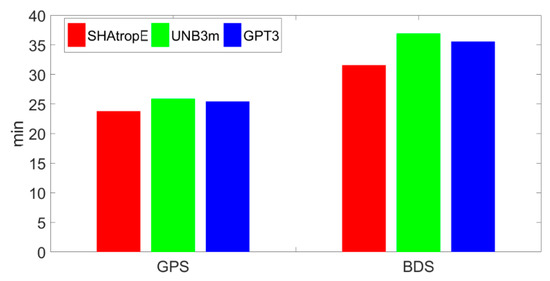
Figure 12.
Average convergence time of static PPP with three different tropospheric models (SHAtropE (red), UNB3m (green), and GPT3 (blue)) for the GPS-only and BDS-only solutions.
5. Conclusions
This study presents a regional ZTD empirical model, SHAtropE, for the regions of [70°E–135°E, 18°N–54°N]. The SHAtropE is a gridded model with a resolution of 2.5° × 2.0°, where at each grid SHAtropE provides users with five periodical ZTD functional parameters (A0,e, A1,e, d1, A2,e, d2) together with five uncertainty functional parameters parameters (B0, B1, f1, B2, f2). Users could derive their local functional parameters by bilinear interpolation and calculate the ZTD over ellipsoid. By applying the derived tropospheric scale height H0 in this study, the ZTD over ellipsoid can be coverted to the true ZTD over site height.
Using 7 years’ data of 310 GNSS sites, the new model is derived and comprehensively validated. Results show that the ZTD precision of SHAtropE is of 3.5 cm in RMS, which has a mean improvement of 35.2% and 5.4% over the UNB3m and GPT3 models, respectively. SHAtropE also provides the predicted ZTD uncertainty, which is valuable when constraining the ZTD in PPP for faster convergence. By applying the SHAtropE model in the static PPP, the convergence time of GPS-only and BDS-only solutions is reduced by 8.1%/14.5% compared to the UNB3m model, and the reduction is 6.9%/11.2% for the GPT3 model.
The input of the SHAtropE is site location (longitude, latitude, ellipsoidal height) and day of the year, and neither temperature and pressure nor humidity measurements are required for the implementation of the model. Thus, its implementation is rather convenient. It is provided in an ASCII-file (30 KB with resolution of 2.5° (Longitude) × 2.0° (Latitude)) containing 10 parameters for each grid and is available at the SHA webpage (www.shao.ac.cn/sha_gnss_ac).
Author Contributions
Conceptualization, J.C.; Funding acquisition, J.C.; Methodology, J.C. and J.W.; Project administration, J.C.; Software, J.W., A.W. and Y.Z.; Supervision, J.C.; Validation, J.W., A.W., J.D. and Y.Z.; Visualization, J.W., A.W. and J.D.; Writing—original draft, J.C.; Writing—review & editing, J.C., J.W., A.W., J.D. and Y.Z. All authors have read and agreed to the published version of the manuscript.
Funding
This research is supported by the National Natural Science Foundation of China (No.11673050); the Key Program of Special Development funds of Zhangjiang National Innovation Demonstration Zone (Grant No. ZJ2018-ZD-009); National Key R&D Program of China (No. 2018YFB0504300); and the Key R&D Program of Guangdong province (No. 2018B030325001).
Acknowledgments
We would like to thank IGS, NGL and CMONOC authorities for providing data for this study.
Conflicts of Interest
The authors declare no conflict of interest.
References
- Böhm, J.; Schuh, H. Atmospheric Effects in Space Geodesy; Böhm, J., Schuh, H., Eds.; Springer: Berlin, Germany, 2013; pp. XVII, 234. [Google Scholar]
- MacMillan, D.S.; Ma, C. Evaluation of very long baseline interferometry atmospheric modeling improvements. J. Geophys. Res. Solid Earth 1994, 99, 637–651. [Google Scholar] [CrossRef]
- Fernandes, M.J.; Lazaro, C.; Ablain, M.; Pires, N. Improved wet path delays for all ESA and reference altimetric missions. Remote Sens. Environ. 2015, 169, 50–74. [Google Scholar] [CrossRef]
- Wu, Z.; Wang, J.; Liu, Y.; He, X.; Liu, Y.; Xu, W. Validation of 7 Years in-Flight HY-2A Calibration Microwave Radiometer Products Using Numerical Weather Model and Radiosondes. Remote Sens. 2019, 11, 1616. [Google Scholar] [CrossRef]
- Bevis, M.; Businger, S.; Herring, T.A.; Rocken, C.; Anthes, R.A.; Ware, R.H. GPS Meteorology—Remote Sensing of Atmospheric Water Vapor Using the Global Positioning System. J. Geophys. Res. Atmos. 1992, 97, 15787–15801. [Google Scholar] [CrossRef]
- Hobiger, T.; Ichikawa, R.; Takasu, T.; Koyama, Y.; Kondo, T. Ray-traced troposphere slant delays for precise point positioning. Earth Planets Space 2008, 60, e1–e4. [Google Scholar] [CrossRef]
- Yao, Y.; Yu, C.; Hu, Y. A New Method to Accelerate PPP Convergence Time by using a Global Zenith Troposphere Delay Estimate Model. J. Navig. 2014, 67, 899–910. [Google Scholar] [CrossRef]
- Lu, C.; Li, X.; Zus, F.; Heinkelmann, R.; Dick, G.; Ge, M.; Wickert, J.; Schuh, H. Improving BeiDou real-time precise point positioning with numerical weather models. J. Geod. 2017, 91, 1019–1029. [Google Scholar] [CrossRef]
- Yao, Y.; Peng, W.; Xu, C.; Cheng, S. Enhancing real-time precise point positioning with zenith troposphere delay products and the determination of corresponding tropospheric stochastic models. Geophys. J. Int. 2017, 208, 1217–1230. [Google Scholar] [CrossRef]
- Zheng, F.; Lou, Y.; Gu, S.; Gong, X.; Shi, C. Modeling tropospheric wet delays with national GNSS reference network in China for BeiDou precise point positioning. J. Geod. 2017, 92, 545–560. [Google Scholar] [CrossRef]
- Wang, J.; Liu, Z. Improving GNSS PPP accuracy through WVR PWV augmentation. J. Geod. 2019. [Google Scholar] [CrossRef]
- Andrei, C.-O.; Chen, R. Assessment of time-series of troposphere zenith delays derived from the Global Data Assimilation System numerical weather model. GPS Solut. 2008, 13, 109–117. [Google Scholar] [CrossRef]
- Chen, Q.; Song, S.; Heise, S.; Liou, Y.-A.; Zhu, W.; Zhao, J. Assessment of ZTD derived from ECMWF/NCEP data with GPS ZTD over China. GPS Solut. 2011, 15, 415–425. [Google Scholar] [CrossRef]
- Hopfield, H.S. Two-quartic tropospheric refractivity profile for correcting satellite data. J. Geophys. Res. 1969, 74, 4487–4499. [Google Scholar] [CrossRef]
- Saastamoinen, J. Atmospheric Correction for the Troposphere and Stratosphere in Radio Ranging Satellites. In The Use of Artificial Satellites for Geodesy; Henriksen, S.W., Mancini, A., Chovitz, B.H., Eds.; American Geophysical Union: Washington, DC, USA, 1972; pp. 247–251. [Google Scholar]
- Collins, J.P.; Langley, R.B. A Tropospheric Delay Model for the User of the Wide Area Augmentation System; Department of Geodesy and Geomatics Engineering, University of New Brunswick: Fredericton, NB, Canada, 1997. [Google Scholar]
- Leandro, R.F.; Langley, R.B.; Santos, M.C. UNB3m_pack: A neutral atmosphere delay package for radiometric space techniques. GPS Solut. 2007, 12, 65–70. [Google Scholar] [CrossRef]
- Penna, N.; Dodson, A.; Chen, W. Assessment of EGNOS tropospheric correction model. J. Navig. 2001, 54, 37–55. [Google Scholar] [CrossRef]
- Boehm, J.; Heinkelmann, R.; Schuh, H. Short Note: A global model of pressure and temperature for geodetic applications. J. Geod. 2007, 81, 679–683. [Google Scholar] [CrossRef]
- Kouba, J. Testing of global pressure/temperature (GPT) model and global mapping function (GMF) in GPS analyses. J. Geod. 2009, 83, 199–208. [Google Scholar] [CrossRef]
- Lagler, K.; Schindelegger, M.; Bohm, J.; Krasna, H.; Nilsson, T. GPT2: Empirical slant delay model for radio space geodetic techniques. Geophys. Res. Lett. 2013, 40, 1069–1073. [Google Scholar] [CrossRef]
- Böhm, J.; Möller, G.; Schindelegger, M.; Pain, G.; Weber, R. Development of an improved empirical model for slant delays in the troposphere (GPT2w). GPS Solut. 2015, 19, 433–441. [Google Scholar] [CrossRef]
- Landskron, D.; Böhm, J. VMF3/GPT3: Refined discrete and empirical troposphere mapping functions. J. Geod. 2017, 92, 349–360. [Google Scholar] [CrossRef]
- Askne, J.; Nordius, H. Estimation of tropospheric delay for microwaves from surface weather data. Radio Sci. 1987, 22, 379–386. [Google Scholar] [CrossRef]
- Li, W.; Yuan, Y.; Ou, J.; Li, H.; Li, Z. A new global zenith tropospheric delay model IGGtrop for GNSS applications. Chin. Sci. Bull. 2012, 57, 2132–2139. [Google Scholar] [CrossRef]
- Li, W.; Yuan, Y.; Ou, J.; Chai, Y.; Li, Z.; Liou, Y.-A.; Wang, N. New versions of the BDS/GNSS zenith tropospheric delay model IGGtrop. J. Geod. 2014, 89, 73–80. [Google Scholar] [CrossRef]
- Yao, Y.; Hu, Y.; Yu, C.; Zhang, B.; Guo, J. An improved global zenith tropospheric delay model GZTD2 considering diurnal variations. Nonlinear Process. Geophys. 2016, 23, 127–136. [Google Scholar] [CrossRef]
- Yao, Y.; Zhang, B.; Xu, C.; He, C.; Yu, C.; Yan, F. A global empirical model for estimating zenith tropospheric delay. Sci. China Earth Sci. 2015, 59, 118–128. [Google Scholar] [CrossRef]
- Chen, J.; Wu, B.; Hu, X.; Li, H. SHA: The GNSS Analysis Center at SHAO. China Satell. Navig. Conf. (CSNC) 2012 Proc. 2012, 160, 213–221. [Google Scholar] [CrossRef]
- Blewitt, G.; Hammond, W.; Kreemer, C. Harnessing the GPS Data Explosion for Interdisciplinary Science. Eos 2018, 99. [Google Scholar] [CrossRef]
- Rzepecka, Z. Time series analysis of radio signal WET tropospheric delays for short-term forecast. Acta Geodyn. Geomater. 2015, 345–354. [Google Scholar] [CrossRef]
- Chen, J.; Zhang, Y.; Zhou, X.; Pei, X.; Wang, J.; Wu, B. GNSS clock corrections densification at SHAO: From 5 min to 30 s. Sci. China Phys. Mech. Astron. 2013, 57, 166–175. [Google Scholar] [CrossRef]
- Wang, J.; Junping, C.; Jiexian, W.; Jiejun, Z.; Lei, S. Assessment of Tropospheric Delay Correction Models over China. Geomat. Inf. Sci. Wuhan Univ. 2016, 41, 1656–1663. [Google Scholar]
- Jin, S.; Park, J.-U.; Cho, J.-H.; Park, P.-H. Seasonal variability of GPS-derived zenith tropospheric delay (1994–2006) and climate implications. J. Geophys. Res. 2007, 112. [Google Scholar] [CrossRef]
- Lou, Y.; Huang, J.; Zhang, W.; Liang, H.; Zheng, F.; Liu, J. A New Zenith Tropospheric Delay Grid Product for Real-Time PPP Applications over China. Sensors 2017, 18, 65. [Google Scholar] [CrossRef] [PubMed]
- Wang, J.; Wu, Z.; Semmling, M.; Zus, F.; Gerland, S.; Ramatschi, M.; Ge, M.; Wickert, J.; Schuh, H. Retrieving Precipitable Water Vapor From Shipborne Multi-GNSS Observations. Geophys. Res. Lett. 2019, 46, 5000–5008. [Google Scholar] [CrossRef]
- Janssen, V.; Ge, L.; Rizos, C. Tropospheric corrections to SAR interferometry from GPS observations. GPS Solut. 2004, 8, 140–151. [Google Scholar] [CrossRef]
- Boehm, J.; Niell, A.; Tregoning, P.; Schuh, H. Global Mapping Function (GMF): A new empirical mapping function based on numerical weather model data. Geophys. Res. Lett. 2006, 33. [Google Scholar] [CrossRef]
- Petit, G.; Luzum, B. IERS Conventions (2010) (IERS Technical Note No. 36); IERS: Frankfurt am Main, Germany, 2010. [Google Scholar]
- Wu, J.T.; Wu, S.C.; Hajj, G.A.; Bertiger, W.I.; Lichten, S.M. Effects of Antenna Orientation on GPS Carrier Phase. Manuscr. Geod. 1993, 18, 91–98. [Google Scholar]
- Guo, F.; Li, X.; Zhang, X.; Wang, J. Assessment of precise orbit and clock products for Galileo, BeiDou, and QZSS from IGS Multi-GNSS Experiment (MGEX). GPS Solut. 2016, 21, 279–290. [Google Scholar] [CrossRef]


© 2020 by the authors. Licensee MDPI, Basel, Switzerland. This article is an open access article distributed under the terms and conditions of the Creative Commons Attribution (CC BY) license (http://creativecommons.org/licenses/by/4.0/).