Article

Generating High Resolution LAI Based on a Modified FSDAF Model

Key Laboratory of Geographical Processes and Ecological Security in Changbai Mountains, Ministry of Education, School of Geographical Sciences, Northeast Normal University, Renmin Street No.5268, Changchun 130024, China
*
Author to whom correspondence should be addressed.
Remote Sens. 2020, 12(1), 150; https://doi.org/10.3390/rs12010150
Submission received: 29 November 2019 / Revised: 20 December 2019 / Accepted: 25 December 2019 / Published: 2 January 2020

Abstract

:
Leaf area index (LAI) is an important parameter for monitoring the physical and biological processes of vegetation canopy. Due to the constraints of cloud contamination, snowfall, and instrument conditions, most of the current satellite remote sensing LAI products have lower resolution that cannot satisfy the needs of vegetation remote sensing application in areas of high heterogeneity. We proposed a new model to generate high resolution LAI, by combining linear pixel unmixing and the Flexible Spatiotemporal Data Fusion (FSDAF) method. This method derived the input data of FSDAF by downscaling the MODIS (Moderate Resolution Imaging Spectroradiometer) data with a linear spectral mixture model. Through the improved input parameters of the algorithm, the fusion of MODIS LAI and LAI at Landsat spatial resolution estimated by Support Vector Regression model was realized. The fusion accuracy of generated LAI data was validated based on Sentinel-2 LAI products. The results showed that strong correlation between predicted LAI and Sentinel-2 LAI in sample sites was observed with higher correlation coefficients and lower Root Mean Square Error. Compared to the simulation results of FSDAF, the modified FSDAF model showed higher accuracy and reflected more spatial details in the boundary areas of different land cover types.

1. Introduction

Leaf Area Index (LAI) is defined as half of the total area of vegetation leaves per unit area [1,2]. As a key parameter to characterize the structural characteristics of vegetation canopy, LAI not only affects biophysical processes such as plant photosynthesis, soil respiration, surface evapotranspiration, and so forth, but completes the regulation of material and energy exchange between vegetation and atmosphere. Accurate LAI data is the prerequisite for understanding and evaluating vegetation growth and the carbon cycle, which is of great significance to maintain ecological balance and improve vegetation productivity.
Satellite remote sensing provides an important method to obtain large scale vegetation canopy LAI. With their diversity and practicability, the current LAI products, such as VEGETATION [3] and Moderate Resolution Imaging Spectroradiometer (MODIS) [4] are helpful to vegetation monitoring [5]. The MODIS LAI product has a high temporal resolution (8-day or 4-day composite), however, the low spatial resolution of 1 km or 500 m may not be conducive to quantifying small-scale ecological processes [6]. LAI data with fine spatial resolution can be obtained from the inversion of high resolution surface reflectance data (e.g., Landsat). After extracting LAI with both similar and high-quality from MODIS data, Gao et al. established a regression tree model between Landsat surface reflectance and LAI to generate 30-m resolution LAI [7]. Based on the radiative transfer model, PROSAIL, Li et al. took the vegetation index derived from Landsat data as an input parameter and used the look-up table (LUT) algorithm for LAI inversion [8]. Ganguly et al. proposed a physical inversion algorithm of LAI from Landsat surface reflectance, which parameterized the Bidirectional Reflectance Factor (BRF) as a function of spatial resolution and wavelength based on the canopy spectral invariants theory [6]. However, due to cloud contamination, the Landsat 16-day revisit cycle may be extended, which can be a major obstacle for monitoring continuous changes in vegetation LAI [9].
Data fusion provide an effective way to integrate satellite observations with various spatial and temporal resolution to obtain high-resolution continuous data. The spatial and temporal adaptive reflectance fusion model (STARFM) proposed by Gao et al. (2006) is one of the most widely used data fusion models, which blends MODIS daily surface reflectance data and the 16-day Landsat Enhanced Thematic Mapper Plus (ETM+) surface reflectance to generate a synthetic daily surface reflectance with spatial resolution of 30 m [10,11,12]. The STARFM algorithm is useful in detecting gradual changes in large areas, however, it has limitations when the changes are transient and not recorded in the base Landsat images. The Spatial Temporal Adaptive Algorithm for mapping Reflectance Change (STAARCH) spatiotemporal fusion algorithm [13] can identify the spatial and temporal variations of the landscape with more details. Since the STARFM might not be very sensitive in heterogeneous landscapes, Zhu et al. (2010) proposed the enhanced STARFM model (ESTARFM), which assumed the reflectance of an object linearly changed over a period of time and the value of the mixed pixel was the linear combination of the spectral reflectance of different objects. A conversion coefficient was introduced in the ESTARFM model so that the accuracy of data fusion in fragmental areas would improve [14]. Like the STARFM, the ESTARFM cannot predict the changes along the boundaries of different objects over time and requires more input data. In 2016, Zhu et al. proposed the Flexible Spatial and Temporal Adaptive Reflectance Fusion Model (FSDAF), which only required two low-resolution images and one high-resolution image to predict modifications and conversions of land cover [15]. The FSDAF model is suitable for heterogeneous landscapes and can maintain more spatial details [16]. It can not only capture the changes in reflectance caused by land cover types conversion, but increase the availability of high-resolution time series data. The FSDAF method can be used to detect rapid land surface changes and solve the problem of the low accuracy of fusion image caused by land feature changes to some extent. Yang et al. (2018) [17] used the FSDAF method to blend MODIS and Advanced Spaceborne Thermal Emission Reflection Radiometer (ASTER) data and generate high spatial and temporal resolution land surface temperature (LST) data with clear texture and high accuracy. Wang et al. (2017) [18] explored the relationship between vegetation coverage and vegetation index from Landsat Thematic Mapper (TM) images generated by the FSDAF method and obtained time series Normalized Differential Vegetation Index (NDVI) with high availability. Zhang et al. (2017) [19] fused Landsat and MODIS data with FSDAF method to predict dense time series NDVI and LST data, which could fill the data gaps caused by clouds, rainfall, etc. However, when big differences exist between two MODIS images for data fusion, the accuracy of the predicted data will decrease accordingly. Moreover, the problem of mixed pixels at the junction of different land cover types of low-resolution image cannot be well solved, thus affecting the accuracy of fusion results.
In the FSDAF model, the low-resolution images are resampled as input data, which lead to certain errors in areas of high heterogeneity. The downscaling of the input image may solve this problem. In the Spatio-Temporal Enhancement Method for medium resolution LAI (STEM-LAI) proposed by Houborg et al. [20], the STARFM model was used to blend a downscaled 250 m LAI and 30 m LAI to generate images with accuracy higher than 1km as input data. In this study, we present a data fusion method combining linear pixel unmixing and the FSDAF model. Based on MODIS LAI products (i.e., MOD15A2H) and the Landsat-8 Operational Land Imager (OLI) images, MODIS LAI data are downscaled through linear spectral mixture model. The downscaling LAI data are used to replace the resampled low-resolution data in the FSDAF, and then are fused with Landsat LAI data retrieved by support vector regression (SVR) model to generate high spatial and temporal resolution LAI data. Finally, the predicted LAI data by the proposed modified method and the FSDAF model were validated by using the synchronous Sentinel-2 LAI data and retrieved Landsat LAI as the real images. By comparison, this modified FSDAF model shows higher accuracy of fusion results and help obtain high spatial and temporal data for the high heterogenous landscape.

2. Methods

2.1. Downscaling of MODIS LAI Data Based on Linear Spectral Unmixing

A linear spectral mixture model was adopted to downscale MODIS LAI data in this study. Linear mixing is the special case of nonlinear mixing ignoring the multiple scattering. The linear model assumes that the reflectance of a mixed pixel is a linear combination of the reflectance of the pixel endmember and its proportion in the mixed pixel [21]. The ratio of the reflectance of each endmember in a pixel is determined by the area ratio (i.e., abundance) of the object in the pixel. Similarly, LAI of a mixed pixel may also be composed of LAI of different land cover categories and their proportions. Therefore, LAI of the mixed pixel can be expressed as
L A I i = j = 1 n ( f j ( i , j ) × l a i j ¯ ) + ε i
in which i is index of a mixed pixel, j is the categories which the endmember belongs to within the mixed pixel (j = 1,…, n), L A I i represents the LAI of the i t h mixed pixel, l a i j ¯ is the average LAI of class j within the mixed pixel, f j ( i , j ) is the abundance of class j , and ε i is the residual error, respectively. Since the adjacent pixels of the same category may have the same or similar LAI, we assume that the LAI of decomposed higher resolution homogeneous pixels belonging to class j ( l a i j ) are equal to l a i j ¯ . The abundance can be calculated by the land cover classification map of 30-m resolution [6]:
f j ( i , j ) = C S Constrained : j = 1 n f j ( i , j ) = 1 , 0 < f j ( i , j ) < 1
in which C is the number of land cover categories in a mixed pixel, and S is the total number of land cover categories in the whole MODIS image. In Equation (1), L A I i and f j ( i , j ) is known, and the constrained least square method is used to solve the linear equations to calculate the average LAI of the class j in the mixed pixels. Due to the needs of the least square theory, Equation (1) is carried out within a window of a certain size. The window can not only eliminate the effects of matching errors among high resolution images [22], but also reflect the spatial differences in similar surface objects [23]. The average LAI of different categories in the mixed pixels within the window are calculated and are assigned to the pixels of corresponding category according to land cover map, thereby the high resolution LAI data are obtained.

2.2. Retrieval of LAI from Landsat Images

In this study, the homogenous pure pixel filtering method proposed by Zhou et al. [24] was used to construct Support Vector Regression (SVR) model for LAI inversion, by taking high quality MODIS reflectance and LAI data as the training samples. We selected high-quality LAI data according to the following steps: (1) Masking MODIS LAI data with land cover classification products and extracting the pixels of cropland during the study period as the sample pixels; (2) Using MODIS LAI QC_Layer to ensure the retrieval of high quality LAI pixels from the main algorithm (i.e., look-up table algorithm); (3) Filtering the remaining LAI pixels through the variation coefficient (CV) and selecting the homogeneous pure pixels.
Support Vector Regression (SVR) is a machine learning method, which uses a finite sample to construct a decision function in a high dimensional feature space to implement linear regression. SVR intends to build an optimal spectral channel, which can not only provide as much data as possible within a given accuracy range ( ε ), but expect the distance between the sample points and the edge of the channel to be no greater than ε [25]. The regression equation can be expressed as Equation (3):
f ( x ) = ( ω , φ ( x , x i ) ) + b
where ω is the coefficient vector, x i represents the support vector, φ ( x , x i ) is the mapping function of x i , and b is the deviation of the function.
Since the selection of parameters has a great influence on the quality of the final model, the cross-validation method can be used to determine the optimal parameters for regression. SVR needs to select an appropriate kernel function according to data characteristics. In this study, Radial Basis Function (RBF) was adopted to map data into high-dimensional feature space and the nonlinear relationship between LAI and reflectance could be revealed better. The more training data are used, the closer the predicted values by SVR are to the true data. Therefore, we used the training samples to develop the conversion model between LAI and spectral reflectance through SVR. After that, Landsat reflectance was used as the input to estimate 30-m resolution LAI.

2.3. The Modified FSDAF Model

As a kind of spatio-temporal data fusion model, the input data of the original FSDAF method includes a pair of low-resolution images at the start time ( t 1 ) and the predicted time ( t 2 ) and a high-resolution image at the same start time ( t 1 ) . The FSDAF model requires the above images to be the same physical variable, such as land surface reflectance or apparent reflectance at the top of atmosphere. All images have the same projection. Taking a high-resolution image as the reference, the low-resolution image is resampled using nearest neighbor method to the same spatial resolution as the high-resolution images [26]. Furthermore, in order to reduce the differences between low and high resolution data derived from different sensors, the radiation normalization is implemented by assuming a linear relationship between the two kinds of data [12]. FSDAF mainly includes the following six steps: (1) Classifying the high-resolution images at time t 1 by Iterative Self-Organizing Data Analysis Technique Algorithm (ISODATA) method; (2) Detecting the changes of land cover types from t 1 to t 2 based on two low-resolution images; (3) Predicting the high-resolution image at time t 2 according to the temporal changes of each land cover type, and calculating the residuals of each low-resolution pixel; (4) Interpolating the low-resolution image at time t 2 to by the thin plate spline (TPS) function to predict the high-resolution image; (5) Distributing the calculated residual in step (3) to the predicted high-resolution image; (6) Assigning weight using neighborhood information to generate the high-resolution image at the time t 2 [15].
In this paper, the combining linear pixel unmixing and FSDAF fusion model with MODIS and Landsat OLI data was used to estimate high spatio-temporal LAI data. The model can be expressed as follows:
L A I ^ t 2 ( x i j , y i j ) = L A I t 1 ( x i j , y i j ) + k 1 n W k × Δ L A I ( x k , y k )
Δ L A I ( x i j , y i j ) = ε f i n e ( x i j , y i j ) + Δ L A I ( c )
in which i is index of a low-resolution pixel, j is index of a high-resolution pixel in the corresponding low-resolution pixel, and ( x i j , y i j ) is the coordinate index of the jth high resolution pixel within the ith low resolution pixel. k is the index of the similar pixel, which is the neighboring pixel with the same land cover type as the pixel at location ( x i j , y i j ) . L A I ^ t 2 ( x i j , y i j ) is the predicted high resolution LAI data at time t 2 , L A I t 1 ( x i j , y i j ) is the high resolution LAI data at time t 1 , and the weight of the k t h similar pixel is W k [14]. Δ L A I ( x k , y k ) represents the LAI changes between time t 1 and time t 2 of similar pixel. The change information of all similar pixels is weighted to obtain the total change value of the target pixel ( x i j , y i j ) . The final estimate of all change is added to the initial LAI observation at t 1 to obtain the final prediction of the target pixel value at t 2 . In Equation (5), Δ L A I ( c ) is the changed LAI of class c in high resolution data from time t 1 to time t 2 , and ε f i n e ( x i j , y i j ) is the residual assigned to the j t h high resolution pixel in the i t h low resolution pixel. The residual can be computed by the following Equations:
ε f i n e ( x i j , y i j ) = m × L ( x i , y i ) × W ( x i j , y i j )
L ( x i , y i ) = Δ L ( x i , y i ) 1 m [ j = 1 m L A I t 2 T P ( x i j , y i j ) j = 1 m L A I t 1 ( x i j , y i j ) ]
L W ( x i j , y i j ) = E h o ( x i j , y i j ) × H I ( x i j , y i j ) + E h e ( x i j , y i j ) × [ 1 H I ( x i j , y i j ) ]
E h o ( x i j , y i j ) = L A I t 2 S P ( x i j , y i j ) L A I t 2 T P ( x i j , y i j )
L A I t 2 S P ( x i j , y i j ) = f T P S b ( x i j , y i j )
in which m represents the number of the sub-pixels in one low resolution pixel, L ( x i , y i ) is the residual between the observed high resolution LAI and the predicted LAI, Δ L ( x i , y i ) is the changes in LAI of low resolution images from time t 1 to time t 2 , L A I t 2 T P ( x i j , y i j ) is the LAI at time t 2 predicted by temporal changes, and L A I t 2 S P ( x i j , y i j ) is the LAI of each pixel in high resolution image predicted by TPS interpolation function after optimizing the parameter. L W ( x i j , y i j ) is the weight of residual distribution, W ( x i j , y i j ) is the weight after normalizing L W ( x i j , y i j ) , E h o ( x i j , y i j ) is the temporal prediction error, E h e ( x i j , y i j ) is the equal error within a low resolution pixel when the landscape is heterogeneous, H I ( x i j , y i j ) is the homogeneous coefficient, and f T P S ( x i j , y i j ) is the TPS functions. The flowchart is shown in Figure 1.
t1 is the start time and t2 is the predict time of fusion process, TPS is the thin plate spline function.

3. Experiment and Results

3.1. Test Area

The algorithm was tested with agriculture land in Songyuan city, Jilin province, China, between 45°21′–44°55′N and 124°25′–125°1′E. It is characterized by a temperate continental semi-humid and semi-arid monsoon climate. The predominant land cover type is cropland. Other land cover types such as water body, forest, grassland, and built-up land can also be found, showing a high heterogeneity of landscape. In order to avoid the contingency of the experimental results, we selected two sample plots (14.4 km × 14.4 km) in the test Area. The main land cover type in Area A is cropland, interspersed with construction lands, especially several roads. In Area B, grassland and cropland had similar area ratio.

3.2. Data and Preprocessing

For this experiment, we selected MODIS product including LAI (MOD15A2H) and surface reflectance (MOD09A1) from June to September in 2018, 12 images (MODIS tile number: h26, v04) in total. These MODIS data provides 8-day composite data with a spatial resolution of 500 m. MODIS LAI product is estimated from the main algorithm, that is, the Look-up Table (LUT) method, which uses the reflectance of red (0.62–0.67 μm) and near-infrared (NIR) (0.841–0.876 μm) bands, and an alternative algorithm based on the empirical relationship between LAI and vegetation index as well [27]. The LAI quality and algorithm path of each pixel are recorded in the data quality control layer (QC_Layer). The latter three SCF_QC of the quality control field describe the algorithm used for LAI inversion [28]. When the value of SCF_QC is “000”, it indicates that this pixel uses the LUT algorithm and is not saturated.
Both MODIS and Landsat data were collected from the United States Geological Survey website (https://earthexplorer.usgs.gov/). Two cloud-free Landsat-8 OLI images on 1 July 2018 and 2 August 2018 (path 119, row 29) were used to estimate high resolution LAI at starting time. Table 1 shows the spectral wavelength of different sensors. We used green (0.53–0.59 μm), red (0.64–0.67 μm), and NIR (0.85–0.88 μm) bands derived from Landsat OLI, which were similar to the band widths of MODIS data. After radiation calibration and atmospheric correction, Landsat images were resampled to the same resolution as MODIS data.
The European Space Agency’s (ESA) Sentinel-2A mission with the MultiSpectral Instrument (MSI, ESA, Paris, France) onboard was launched in 2015. Sentinel-2A data comprises 13 bands with different spatial resolutions of 10 m, 20 m, and 60 m, which can reflect land surface information accurately. In this experiment, the dates of Sentinel-2A data acquisition were 3 July and 1 August in 2018 (N 0206, R 089), obtained from ESA SciHub website (https://scihub.copernicus.eu/dhus/#/home). Sentinel-2A’s Level-1C (L1C) data have been processed by geographical registration and radiation correction. Sen2Cor [29] atmospheric correction software is used to transform the atmospheric apparent reflectance into surface reflectance (Level-2A) [30]. The processed L2A data were used to estimate LAI by the biophysical module of Sentinel Application Platform (SNAP, ESA, Paris, France [31], and resampled to 30 m resolution. In this study, Sentinel-2A LAI was used to verify the accuracy of the retrieved 30 m resolution LAI from Landsat data and the fusion LAI from the improved FSDAF method.
30-m resolution global land-cover maps in the Finer Resolution Observation and Monitoring of Global Land Cover (FROM-GLC) project was collected from http://data.ess.tsinghua.edu.cn/. Land cover in FROM-GLC product is divided into 10 classes, including agriculture lands, grasslands, shrublands, and bare land, etc. In this study, the land cover map in the year of 2017 was used for the mixed pixels unmixing.

3.3. LAI Inversion from Landsat-8 Data by Support Vector Regression Model

Before performing the SVR analysis, high-quality MODIS LAI and the corresponding reflectance data were selected as training samples. Firstly, land cover data was resampled to the spatial resolution of MODIS data. Cropland LAI were obtained by the masking LAI data using land cover data. Secondly, the quality control layer (FparLai_QC Layer) of MOD15A2 was utilized to select the high-quality pixels by the main algorithm (SCF_QC = 000). At MODIS scale, the Landsat reflectance data were used to calculate the coefficient of variation (CV) (Equation (1)). According to the previous study [7], the pixels with CV value less than 0.15 were regarded as pure pixels. The high-quality pure LAI pixels of cropland were chosen. The same pixels were also selected from surface reflectance (MOD09A1). Finally, the SVR model was established using the selected training samples. Land surface reflectance of red, near-infrared, and green bands were used as input data of SVR model to estimate LAI of 30-m resolution. The quasi synchronization Sentinel-2A LAI data were applied to validate the inversion LAI.
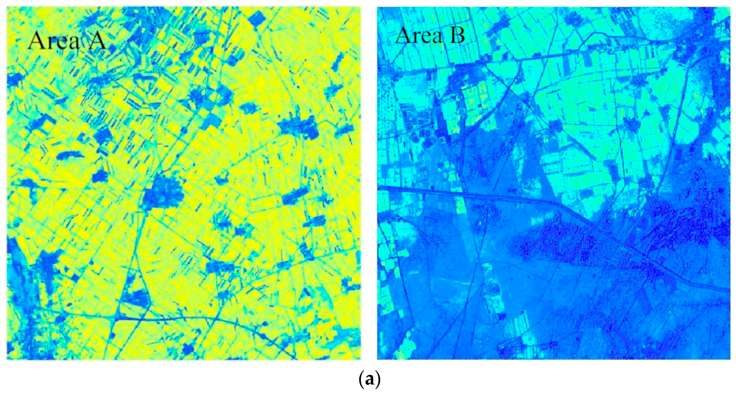
Taking the data on 2 August 2018 as an example (as shown in Figure 2), it can be seen that retrieved LAI from Landsat 8 OLI data and Sentinel-2 LAI showed same spatial distribution pattern. For Area A, estimated LAI varied between 0.2090 and 3.6464, with a mean value and standard deviation of 2.4802 and 1.2187, respectively. Sentinel-2A LAI ranged from 0.2090 to 6.7426 with an average value and standard deviation of 3.6178 and 0.7940, respectively. Compared with the true values, the LAI values retrieved by the SVR model might be somewhat underestimated in the pixels of high LAI. The inversion LAI in Area B ranged from 0.2178 to 3.5742, with mean LAI and its standard deviation of 1.8245 and 0.7702, respectively. In contrast, the Sentinle-2A LAI varied from 0.0016 to 5.8360, with average value and standard deviation of 1.8334 and 0.9821, respectively. The distribution of the observed LAI was more discrete than that of the predicted LAI.
Firstly, the MODIS LAI data were re-projected from the native Sinusoidal projection to the Universal Transverse Mercator (UTM)-WGS84 reference system. MODIS data were resampled to 480 m, making it a multiple of the resolution of Landsat data to perform the decomposition of mixed pixels. The ground control points (GCPs) were selected from Landsat image as the reference image for geometric correction. After that, the existing 30-m land classification data was used to calculate the class abundance. The abundance map and MODIS data were taken as known variables to unmixing the mixed pixels by using the constrained least square method to obtain 30 m MODIS LAI data. Finally, Landsat image and MODIS data were clipped to the same size (480 × 480 pixels) for subsequent fusion processing.
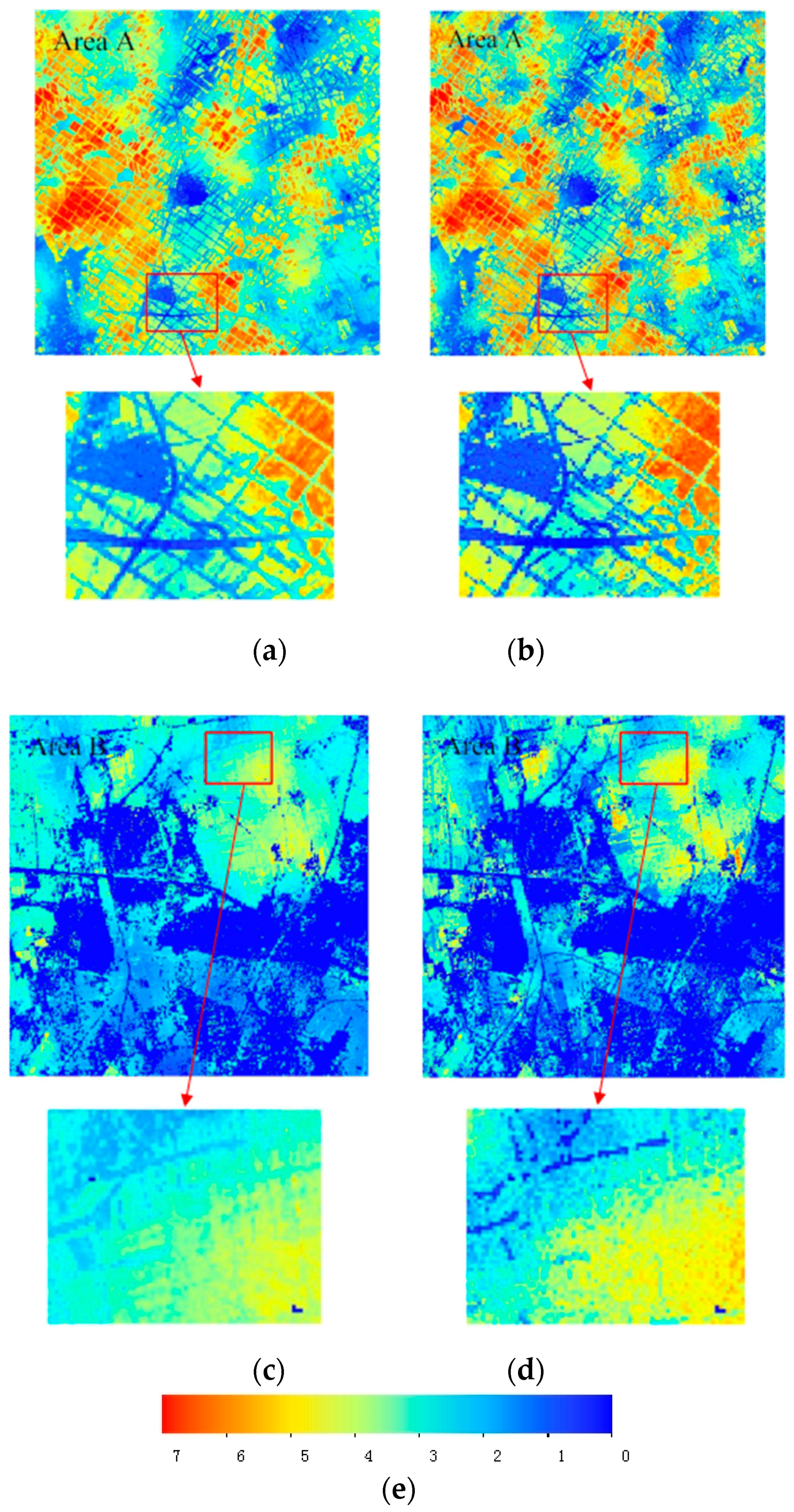
Using the combining linear pixel unmixing and FSDAF fusion model to deal with data, a high-resolution LAI image of prediction time was obtained. The predicted results were compared with the fusion image obtained by the FSDAF model. The MODIS LAI data on 4 July 2018 was taken as the low-resolution image of the starting date. We took the Landsat-8 LAI data on 1 July 2018 as the fine-resolution image of the starting date, and the MODIS LAI image on 5 August 2018 as the low-resolution image of the predicted date. As shown in Figure 3, the predicted images by the two methods could visually reflect spatial and temporal characteristics of LAI. From the enlarged map of the fusion images, LAI generated by the improved FSDAF model showed the internal details and texture information of land objects more clearly.
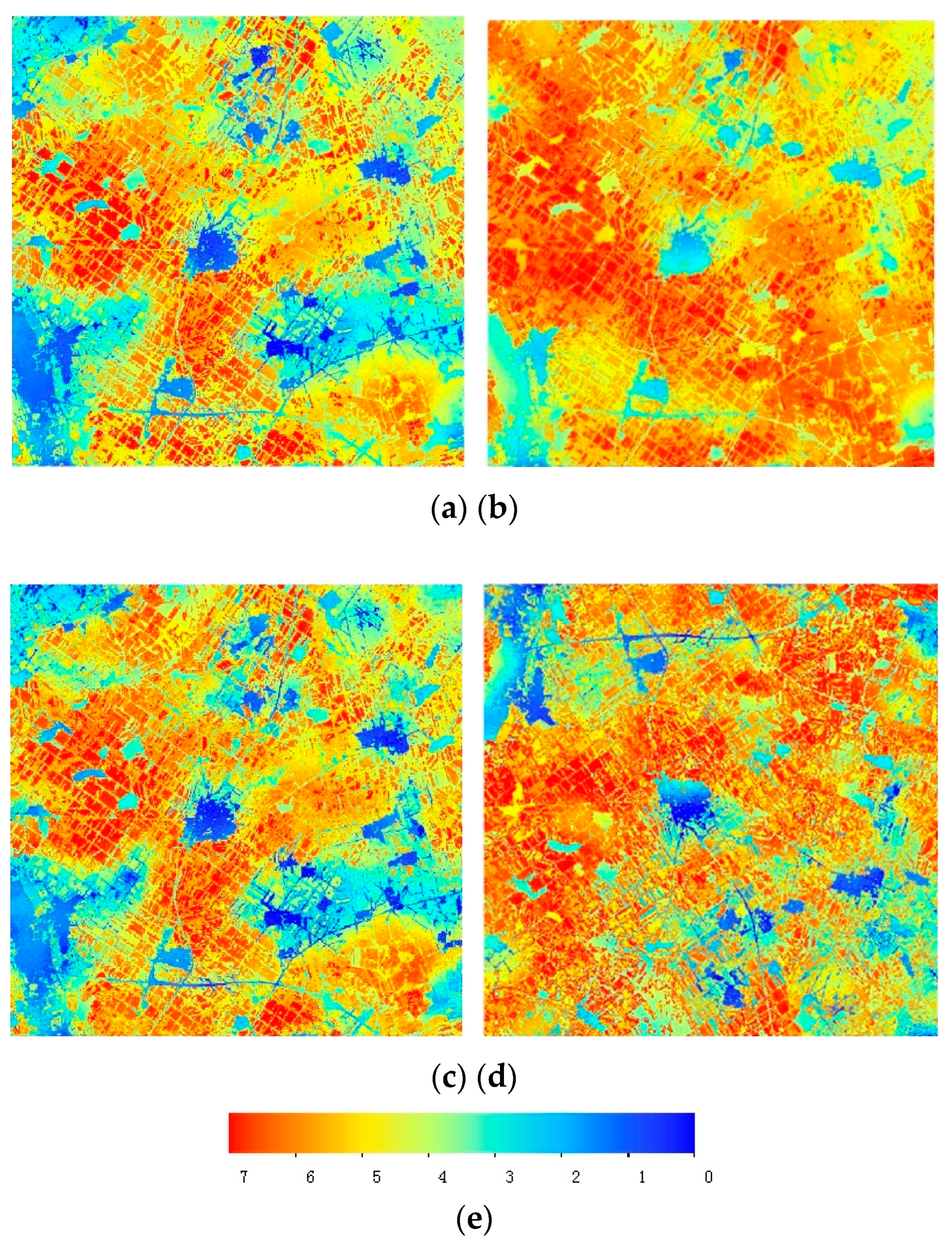
Figure 4 illustrates estimated 30-m resolution LAI of Area A on 20 July and 28 July using the above two models, respectively. The maximum LAI increased from 5.582 to 6.998 during the period, indicating that the predicted data by two fusion models could capture the LAI changes with time. From the LAI of the improved FSDAF model estimation, the regions with lower LAI changed more significantly (Figure 4b). The predicted data on July 28 showed different patterns in the upper left corner and lower middle areas of the study area. LAI of some pixels went up in the improved FSDAF image, but decreased in the original FSDAF image. The predicted high-resolution LAI using the improved FSDAF model showed the obvious temporal differences by decomposing mixed pixels.

4. Discussion

4.1. Analysis of the Accuracy of Landsat LAI Inversion

In order to evaluate the accuracy of inversion, we selected 1000 points randomly from the LAI images in Figure 2. The corresponding LAI values were extracted to establish the fitting relationship between the estimated LAI and true LAI values (Sentinel-2A LAI) (Figure 5). The determination coefficient (R2) and root mean square error (RMSE) were used to measure the similarity between the LAI inversion results and the real image. The greater the R2 and the smaller RMSE, the higher the degree of relevance.
As shown in Figure 5, R2 and the RMSE between Landsat inversion LAI and true LAI for Area A are 0.75347 and 0.89, respectively. The R2 of Area B is 0.88725 with the RMSE of 0.35. The conversion model established by using high-quality MODIS LAI data and the corresponding reflectance data selected by the pure pixel filtering algorithm was applicable to our experimental area and obtained relatively accurate LAI inversion results. It can be seen that most points of the scatter plots are distributed on both sides of y = x. When LAI value is greater than 3, some estimated LAIs are lower than the true values, which is consistent with the research results of Zhou et al. [2]. The retrieved LAI by the SVR model from Landsat images showed high accuracy. In this study, MODIS data at different times were selected as the training samples, which not only involved the characteristics of vegetation during the growing season, but also ensured the diversity and representativeness of the samples. In the process of retrieval, it may be not necessary to consider changed biological characteristics of vegetation due to its growth, thus facilitating the application of the model.

4.2. The Comparison of the Predicted LAI Using the Improved FSDAF and FSDAF Model

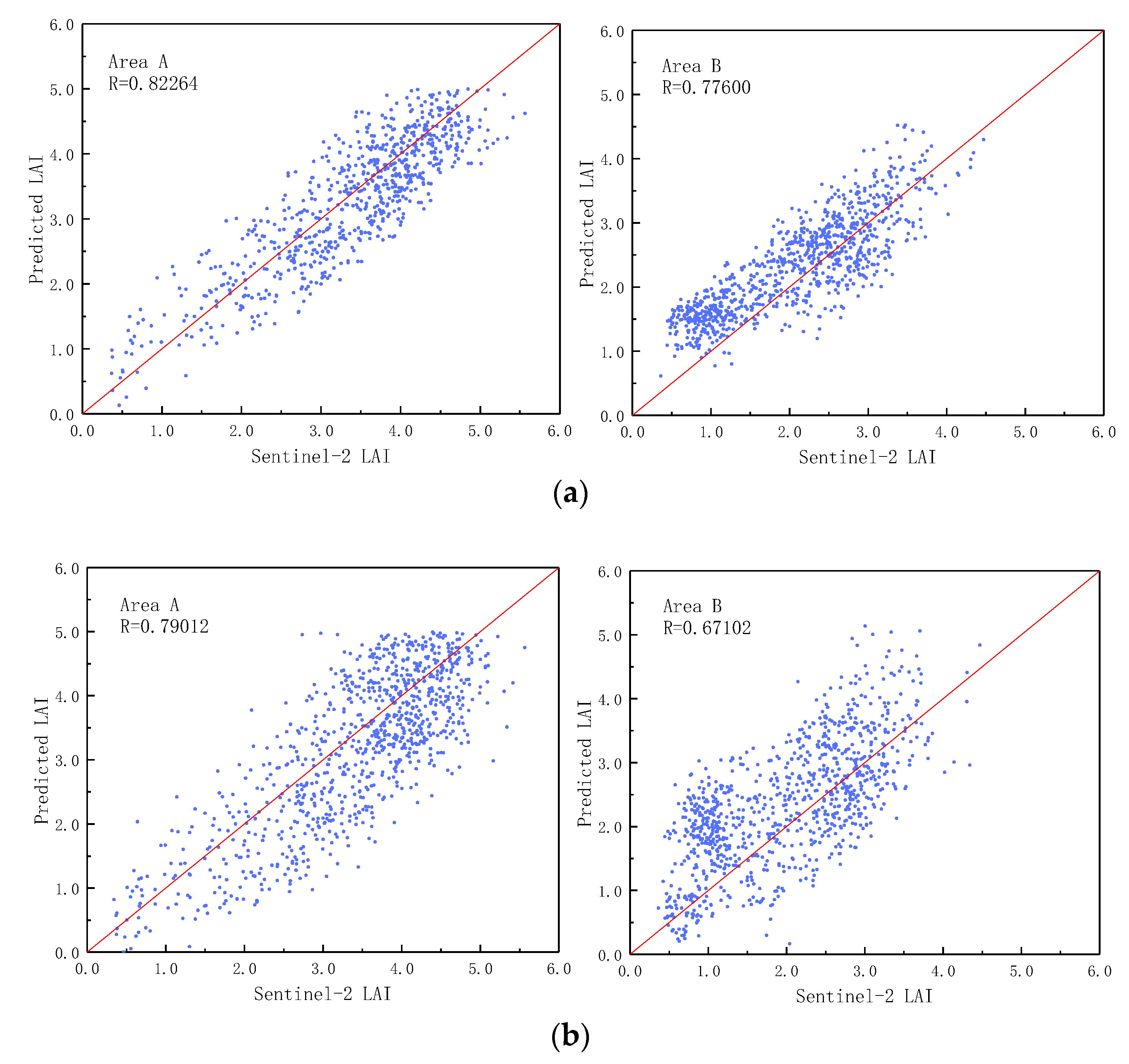
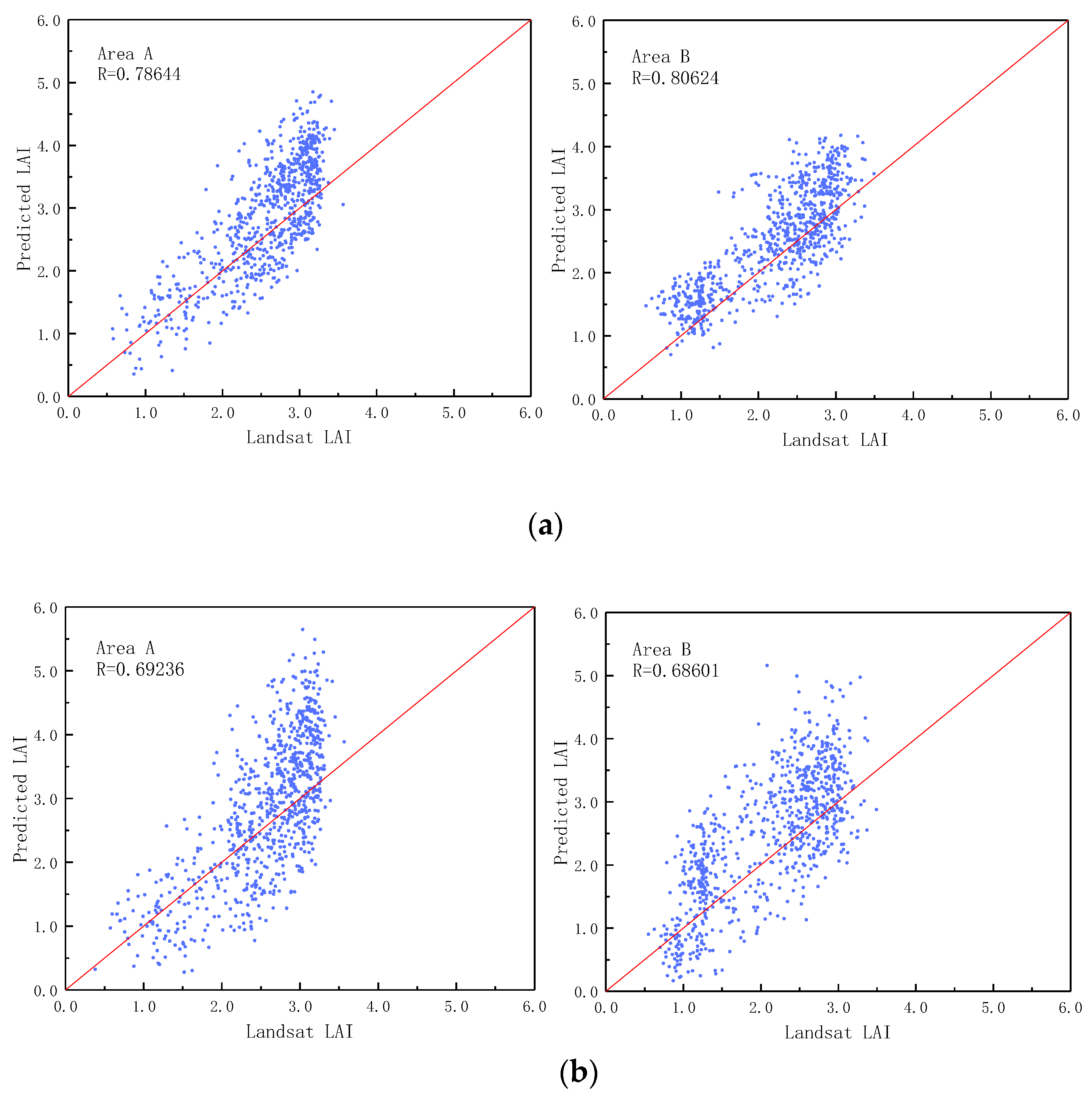
To discuss the validity and reliability of the improved FSDAF method, the predicted LAI were compared with the fusion image obtained by the FSDAF algorithm. Taking Sentinel-2A LAI on August 1 as the reference image, 1000 sample points were randomly selected from the LAI images generated by FSDAF, the improved FSDAF method and the Sentinel-2A data, respectively. The correlation coefficient (R) and RMSE were used to evaluate the effect of LAI fusion. The greater the R value, the better the fusion results. The lower RMSE value stands for the stronger the consistency between fusion result and truth value. Figure 6 illustrates the correlation between the predicted LAI on August 5 and Sentinel-2A LAI product. It can be found that R between the fusion LAI from the improved FSDAF method in Area A is 0.82644, which is higher than that of FSDAF model (0.79012). The RMSE of the improved FSDAF model and FSDAF algorithm are 0.65 and 0.87, respectively. For Area B, the R of the improved FSDAF method and original FSDAF are 0.77600 and 0.67102 with RMSE of 0.67 and 0.98, respectively. Similarly, the correlation between the predicted LAI on August 5 and Landsat LAI retrieved by SVR on August 2 was also shown in Figure 7. The R of the improved FSDAF method at Area A and Area B are 0.78644 and 0.80624, which are higher than those of the FSDAF model (0.69236 and 0.68601). The RMSE of the improved FSDAF model and FSDAF algorithm are 0.69, 0.90 for Area A, and 0.59, 0.92 for Area B, respectively. Table 2 shows the standard difference (SD) of these eight images which can reflect the dispersion of data set. Overall, the predicted LAIs from the improved FSDAF model are better than the fusion result of FSDAF model.
The MODIS data input in the FSDAF method is resampled to 30 m resolution by the nearest neighbor method, thus the value of these resample pixels which belong to the same coarse resolution pixels have strong homogeneity. In fact, there are certain differences between the values of adjacent pixels, especially at the border of different land cover types in the fragmental area. The FSDAF algorithm involves s, the spectral decomposition. The land classification data required for the decomposition is obtained from the fine resolution images by ISODATA method. In our experiment, when FSDAF was applied directly to LAI data fusion, the unsatisfactory effect of land classification might lead to a large error in the unmixing data and lower accuracy of the fusion results. In contrast, the improved FSDAF method performed mixed pixel decomposition on MODIS data at first, which could reflect land surface information more accurately and increase the number of pure pixels. Therefore, the FSDAF algorithm combined the downscaling method of mixed pixel decomposition would improve the accuracy of data fusion.
In the FSDAF proposed by Zhu et al. [15], they conducted two experiments using simulated images and real images, respectively. When the simulated reflectance images were used as input data, the correlation coefficient between the reflectance of fine resolution image and that of the true image on the predicted date was 0.9841, RMSE was 0.0256, and the average difference (AD) was 0.0001. There are two situations when using true images: when land cover types changes occurred on the predicted date, except for the mismatched bands of MODIS and Landsat data, the correlation coefficient of the reflectance of the rest of the six spectral bands (band 1–5, 7) ranged from 0.855 to 0.917 and RMSE varied from 0.01 to 0.04. For the heterogeneous study site, the correlation coefficient and RMSE varied from 0.872 to 0.903 and from 0.014 to 0.045. By contrast, the accuracy of the fusion results in this study was slightly lower. The possible reasons might be as follows: firstly, LAI at Landsat scale was estimated by SVR model. Though the accuracy of the inversion LAI was relatively high, some errors still existed; secondly, the FSDAF fusion model has been mainly used to predict the physical variables such as top of the atmosphere (TOA) reflectance or land surface reflectance so far. When the FSDAF method directly fuses MODIS and Landsat data for generating the biophysical parameters such as LAI, small errors might have been introduced.

4.3. Limitations

The accuracy of low-resolution input data (i.e., MODIS data) has a great influence on the fusion accuracy of the FSDAF model. The existence of mixed pixels is common due to the large field of view of MODIS. In this study, the MODIS data were downscaled using a linear spectral mixture model and then fusion was performed. The estimation accuracy of the improved FSDAF method relies on the accuracy of downscaled MODIS data to some extent. The downscaling method of higher accuracy may achieve better fusion results. In order to estimate LAI from Landsat 8 data, a similar training sample collection method to the previous studies was adopted to conduct support vector regression, which may affect the accuracy of LAI retrieval. The improved FSDAF model can reveal the gradual change of LAI and some transformations between land cover types through the data on starting and predicted dates. However, similar to the FSDAF method, the small transformations of land cover type recorded by low-resolution images of predicted date might not be estimated, which might influence the fusion accuracy. In addition, LAI of cropland decreases significantly after the harvest, thus the fusion algorithm could not obtain precise prediction results.

5. Conclusions

In this paper, an improved spatio-temporal data fusion model which combines FSDAF and linear pixel unmixing method was proposed to fuse Landsat 8 data with MODIS LAI to generate the 30-m resolution LAI data. The following conclusions were drawn:
(1)
A linear spectral mixture model was introduced to downscale the input MODIS data, which replaced the resampled low-resolution data in the FSDAF. This improved FSDAF method can generate high-precision predicted LAI data with high spatiotemporal resolution and is potentially extendable to other biophysical variables prediction.
(2)
The experiments were conducted on two sample sites to avoid the randomness of fusion results. The correlation coefficients between the predicted LAI generated by the data fusion methods and real data are high. The scatter plots of the improved FSDAF model showed a more concentered distribution than that of the FSDAF. The fusion LAI of the improved FSDAF algorithm showed higher accuracy.
(3)
The improved FSDAF method could be applied in highly heterogenous areas. The resultant imagery by the combining linear pixel unmixing and FSDAF model revealed better spatial details and the blurring of the boundaries among different ground objects could be improved.

Author Contributions

H.Z. and F.H. conceptualized the study and designed the research. H.Z. analyzed the data and wrote the paper. F.H. supervised the research and provided significant suggestions. H.Q. was involved in the data processing and the manuscript reviewing. All authors have read and agreed to the published version of the manuscript.

Funding

This research was funded by National Natural Science Foundation of China, grant number 41571405 and 41630749.

Acknowledgments

The authors would like to thank the reviewers and editors for their valuable comments and suggestions.

Conflicts of Interest

The authors declare no conflict of interest.

References

  1. Chen, J.M.; Black, T.A. Defining leaf-area index for non-flat leaves. Agric. For. Meteorol. 2010, 15, 421–429. [Google Scholar] [CrossRef]
  2. Weiss, M.; Baret, F.; Smith, G.J.; Jonckheere, I.; Coppin, P. Review of methods for in situ leaf area index (lai) determination: Part ii. Estimation of lai, errors and sampling. Agric. For. Meteorol. 2004, 121, 37–53. [Google Scholar] [CrossRef]
  3. Baret, F.; Hagolle, O.; Geiger, B.; Bicheron, P.; Miras, B.; Huc, M.; Berthelot, B.; Nino, F.; Weiss, M.; Samain, O.; et al. LAI, fAPAR and fCover CYCLOPES global products derived from VEGETATION—Part 1: Principles of the algorithm. Remote Sens. Environ. 2007, 110, 275–286. [Google Scholar] [CrossRef] [Green Version]
  4. Myneni, R.B.; Hoffman, S.; Knyazikhin, Y.; Privette, J.L.; Glassy, J.; Tian, Y.; Wang, Y.; Song, X.; Zhang, Y.; Smith, G.R.; et al. Global products of vegetation leaf area and fraction absorbed par from year one of modis data. Remote Sens. Environ. 2002, 83, 214–231. [Google Scholar] [CrossRef] [Green Version]
  5. Campos-Taberner, M.; Garcia-Haro, F.J.; Camps-Valls, G.; Grau-Muedra, G.; Nutini, F.; Crema, A.; Boschetti, M. Multitemporal and multiresolution leaf area index retrieval for operational local rice crop monitoring. Remote Sens. Environ. 2016, 187, 102–118. [Google Scholar] [CrossRef]
  6. Ganguly, S.; Nemani, R.R.; Zhang, G.; Hashimoto, H.; Milesi, C.; Michaelis, A.; Wang, W.L.; Votava, P.; Samanta, A.; Melton, F.; et al. Generating global leaf area index from landsat: Algorithm formulation and demonstration. Remote Sens. Environ. 2012, 122, 185–202. [Google Scholar] [CrossRef] [Green Version]
  7. Gao, F.; Anderson, M.C.; Kustas, W.P.; Wang, Y.J. Simple method for retrieving leaf area index from landsat using modis leaf area index products as reference. J. Appl. Remote Sens. 2012, 6. [Google Scholar] [CrossRef]
  8. Li, H.; Chen, Z.X.; Jiang, Z.W.; Wu, W.B.; Ren, J.Q.; Liu, B.; Hasi, T. Comparative analysis of gf-1, hj-1, and landsat-8 data for estimating the leaf area index of winter wheat. J. Integr. Agric. 2017, 16, 266–285. [Google Scholar] [CrossRef]
  9. Wu, M.Q.; Wu, C.Y.; Huang, W.J.; Niu, Z.; Wang, C.Y. High-resolution leaf area index estimation from synthetic landsat data generated by a spatial and temporal data fusion model. Comput. Electron. Agric. 2015, 115, 1–11. [Google Scholar] [CrossRef]
  10. Hilker, T.; Wulder, M.A.; Coops, N.C.; Seitz, N.; White, J.C.; Gao, F.; Masek, J.G.; Stenhouse, G. Generation of dense time series synthetic landsat data through data blending with modis using a spatial and temporal adaptive reflectance fusion model. Remote Sens. Environ. 2009, 1133, 1988–1999. [Google Scholar] [CrossRef]
  11. Emelyanova, I.V.; McVicar, T.R.; Van Niel, T.G.; Li, L.T.; van Dijk, A.I.J.M. Assessing the accuracy of blending landsat-modis surface reflectances in two landscapes with contrasting spatial and temporal dynamics: A framework for algorithm selection. Remote Sens. Environ. 2013, 133, 193–209. [Google Scholar] [CrossRef]
  12. Gao, F.; Masek, J.; Schwaller, M.; Hall, F. On the blending of the landsat and modis surface reflectance: Predicting daily landsat surface reflectance. IEEE Trans. Geosci. Remote 2006, 44, 2207–2218. [Google Scholar]
  13. Hilker, T.; Wulder, M.A.; Coops, N.C.; Linke, J.; McDermid, G.; Masek, J.G.; Gao, F.; White, J.C. A new data fusion model for high spatial- and temporal-resolution mapping of forest disturbance based on landsat and modis. Remote Sens. Environ. 2009, 113, 1613–1627. [Google Scholar] [CrossRef]
  14. Zhu, X.L.; Chen, J.; Gao, F.; Chen, X.H.; Masek, J.G. An enhanced spatial and temporal adaptive reflectance fusion model for complex heterogeneous regions. Remote Sens. Environ. 2010, 114, 2610–2623. [Google Scholar] [CrossRef]
  15. Zhu, X.L.; Helmer, E.H.; Gao, F.; Liu, D.S.; Chen, J.; Lefsky, M.A. A flexible spatiotemporal method for fusing satellite images with different resolutions. Remote Sens. Environ. 2016, 172, 165–177. [Google Scholar] [CrossRef]
  16. Xie, F.D.; Zhang J, H.; Sun P, J.; Pan Y, Z.; Yun, Y.; Yuan Z M, Q. Remote sensing data fusion by combining starfm and downscaling mixed pixel algorithm. J. Remote Sens. 2016, 20, 62–72. [Google Scholar]
  17. Yang, M.; Yang, G.; Chen, X.; Zhang, Y.; You, J.; Agency, S.E. Generation of land surface temperature with high spatial and temporal resolution based on fsdaf method. Remote Sens. Land Resour. 2018, 30, 54–62. [Google Scholar]
  18. Jie, W.; Li, W. Research on relationship between vegetation cover fraction and vegetation index based on flexible spatiotemporal data fusion model. Pratacultural Sci. 2017, 2, 8. [Google Scholar]
  19. Zhang, L.; Weng, Q.H.; Shao, Z.F. An evaluation of monthly impervious surface dynamics by fusing landsat and modis time series in the pearl river delta, China, from 2000 to 2015. Remote Sens. Environ. 2017, 201, 99–114. [Google Scholar] [CrossRef]
  20. Houborg, R.; McCabe, M.F.; Gao, F. A spatio-temporal enhancement method for medium resolution lai (stem-lai). Int. J. Appl. Earth Obs. 2016, 47, 15–29. [Google Scholar] [CrossRef] [Green Version]
  21. Settle, J.J.; Drake, N.A. Linear mixing and the estimation of ground cover proportions. Int. J. Remote Sens. 1993, 14, 1159–1177. [Google Scholar] [CrossRef]
  22. Wu, M.Q.; Niu, Z.; Wang, C.Y.; Wu, C.Y.; Wang, L. Use of modis and landsat time series data to generate high-resolution temporal synthetic landsat data using a spatial and temporal reflectance fusion model. J. Appl. Remote Sens. 2012, 6. [Google Scholar] [CrossRef]
  23. Zhang, W.; Li, A.N.; Jin, H.A.; Bian, J.H.; Zhang, Z.J.; Lei, G.B.; Qin, Z.H.; Huang, C.Q. An enhanced spatial and temporal data fusion model for fusing landsat and modis surface reflectance to generate high temporal landsat-like data. Remote Sens. 2013, 5, 5346–5368. [Google Scholar] [CrossRef] [Green Version]
  24. Zhou, J.M.; Zhang, S.; Yang, H.; Xiao, Z.Q.; Gao, F. The retrieval of 30-m resolution lai from landsat data by combining modis products. Remote Sens. 2018, 10, 1187. [Google Scholar] [CrossRef] [Green Version]
  25. Chang, C.C.; Lin, C.J. Libsvm: A library for support vector machines. ACM Trans. Intell. Syst. Technol. 2011, 2, 27. [Google Scholar] [CrossRef]
  26. Gevaert, C.M.; Garcia-Haro, F.J. A comparison of starfm and an unmixing-based algorithm for landsat and modis data fusion. Remote Sens. Environ. 2015, 156, 34–44. [Google Scholar] [CrossRef]
  27. Ranga Myneni. Modis Collection 6 (c6) Lai/Fpar Product User’s Guide. Available online: https://lpdaac.usgs.gov/sites/default/files/public/product_documentation/mod15_user_guide.pdf (accessed on 1 August 2018).
  28. Yang, W.Z.; Huang, D.; Tan, B.; Stroeve, J.C.; Shabanov, N.V.; Knyazikhin, Y.; Nemani, R.R.; Myneni, R.B. Analysis of leaf area index and fraction of par absorbed by vegetation products from the terra modis sensor: 2000–2005. IEEE Trans. Geosci. Remote 2006, 44, 1829–1842. [Google Scholar] [CrossRef]
  29. Louis, J.; Debaecker, V.; Pflug, B.; Main-Knorn, M.; Gascon, F. Sentinel-2 sen2cor: L2a processor for users. In Proceedings of the Living Planet Symposium, Prague, Czech Republic, 9–13 May 2016. [Google Scholar]
  30. Roy, D.P.; Li, J.; Zhang, H.K.K.; Yan, L.; Huang, H.Y.; Li, Z.B. Examination of sentinel 2a multi-spectral instrument (msi) reflectance anisotropy and the suitability of a general method to normalize msi reflectance to nadir brdf adjusted reflectance. Remote Sens. Environ. 2017, 199, 25–38. [Google Scholar] [CrossRef]
  31. Yang, B.; Li, D.; Wang, L. Retrieval of surface vegetation biomass information and analysis of vegetation feature based on sentinel-2a in the upper of minjiang river. Sci. Technol. Rev. 2017, 35, 74–80. [Google Scholar]
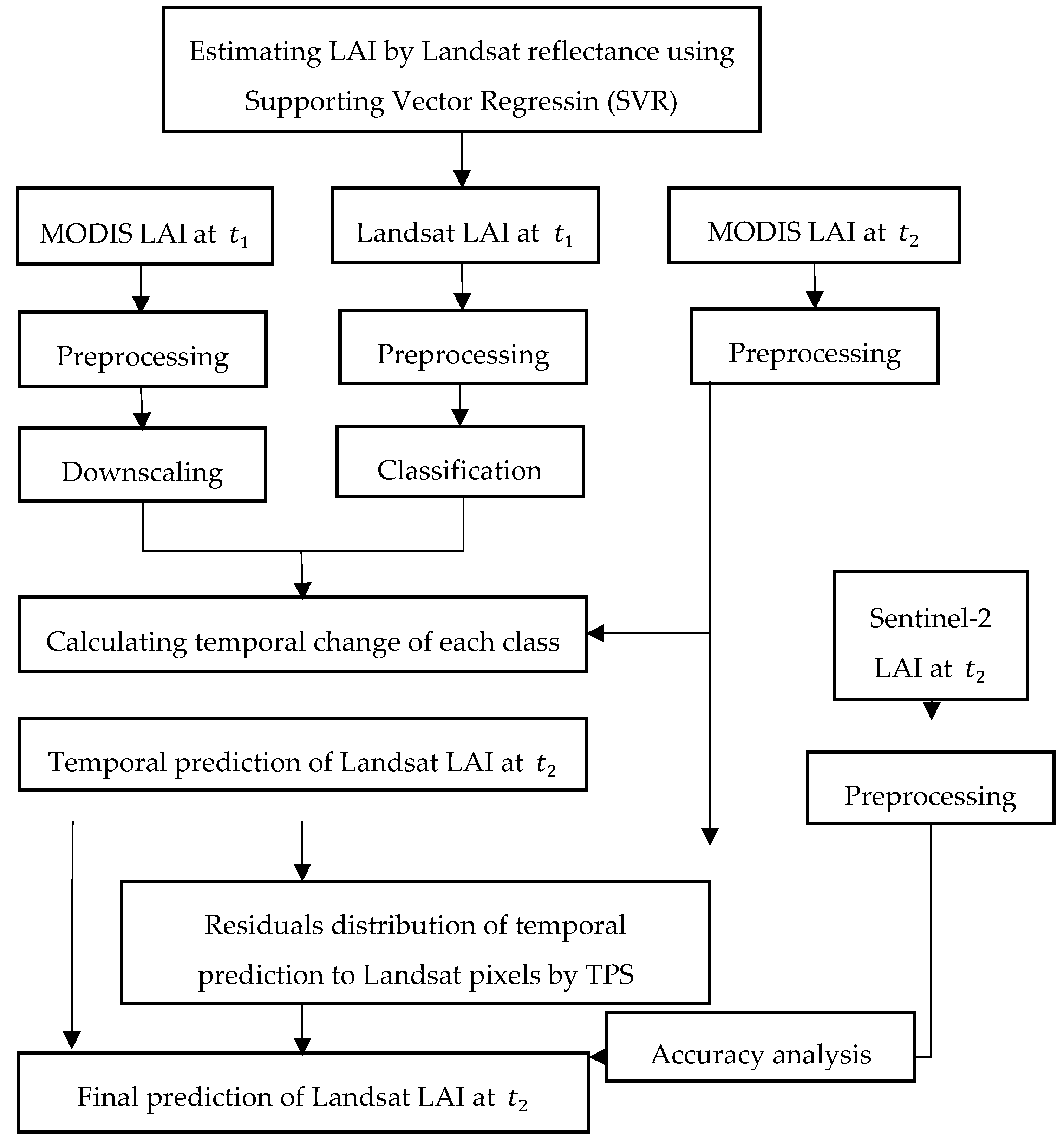
Figure 1. Flowchart of the modified Flexible Spatiotemporal Data Fusion (FSDAF) model.
Remotesensing 12 00150 g001
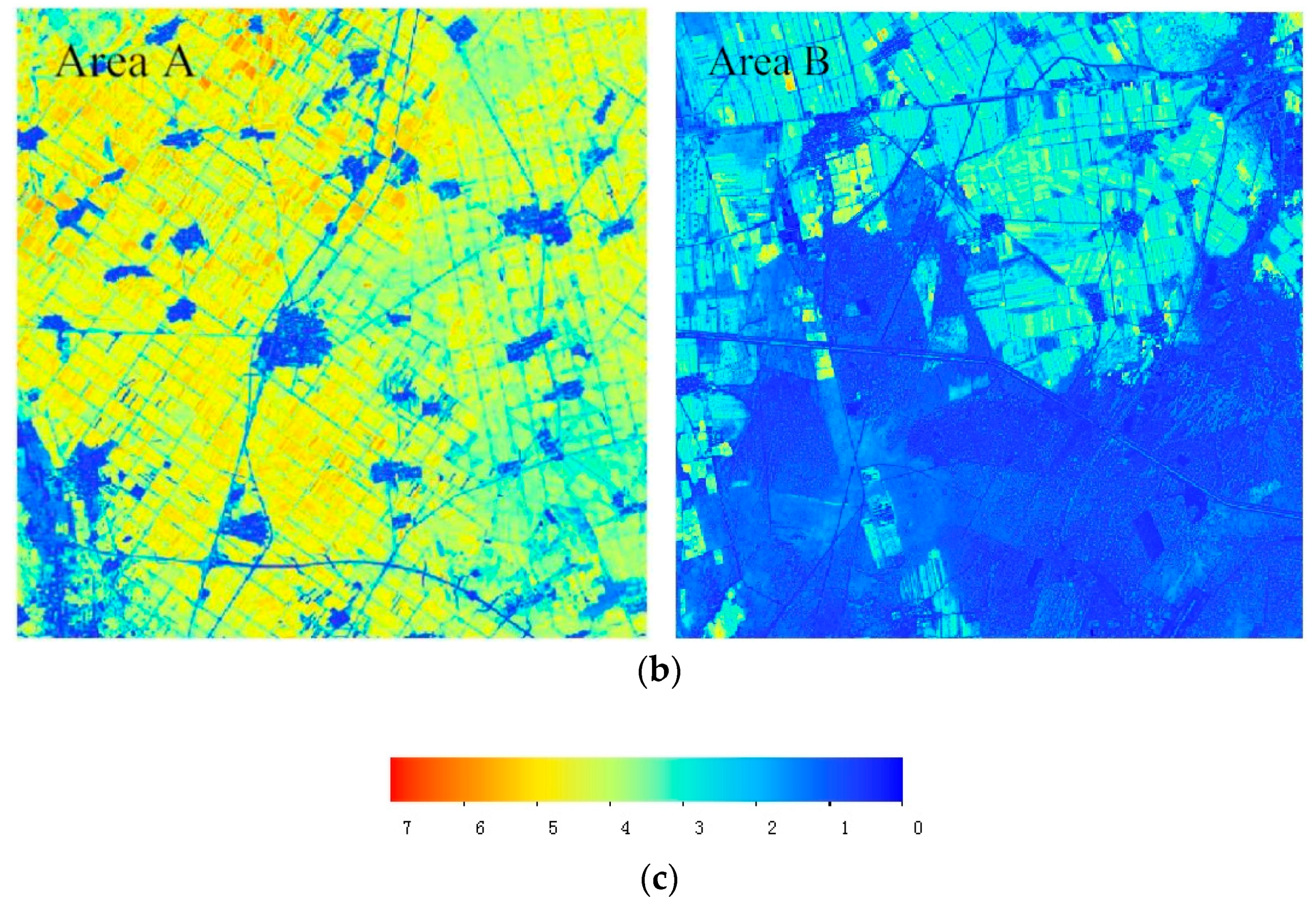
Figure 2. Comparison of Sentinel-2A Leaf Area Index (LAI) data and inversed LAI from Landsat 8 Operational Land Imager (OLI) data. (a) LAI retrieved by support vector regression (SVR) model on 2 August 2018; (b) LAI product of Sentinel-2A on 1 August 2018; (c) the legend of the maps.3.4. Estimation of LAI Using the Improved FSDAF Model.
Remotesensing 12 00150 g002aRemotesensing 12 00150 g002b
Figure 3. Comparison of 30 m LAI on August 5 generated by the improved FSDAF model and the FSDAF method: (a,c) LAI predicted by the improved FSDAF; (b,d) LAI generated from the FSDAF model; (e) the legend of the maps.
Remotesensing 12 00150 g003
Figure 4. The estimated 30 m LAI for Area A on 20 July 2018 and 28 July 2018. (a,b) LAI obtained from the improved FSDAF; (c,d) LAI predicted by FSDAF; (e) the legend of the maps.
Remotesensing 12 00150 g004
Figure 5. The scatter plots of Landsat LAI inversion and Sentinel-2A LAI for different sites. (a) Area A; (b) Area B. (red line is the 1:1 line).
Remotesensing 12 00150 g005
Figure 6. Correlation between the predicted LAI using different fusion models and Sentinel-2 LAI. (a) Improved FSDAF method; (b) FSDAF method. (red line is the 1:1 line).
Remotesensing 12 00150 g006
Figure 7. Correlation between the predicted LAI using different fusion models and Landsat LAI. (a) Improved FSDAF method; (b) FSDAF method. (red line is the 1:1 line).
Remotesensing 12 00150 g007
Table 1. Comparison of band width among different sensors.
BandMODIS(μm)TM(μm)ETM(μm)OLI(μm)
Red0.62–0.670.63–0.690.63–0.690.64–0.67
NIR0.841–0.8760.76–0.900.76–0.900.85–0.88
Blue0.459–0.4790.45–0.520.45–0.520.45–0.51
Green0.545–0.5650.52–0.600.52–0.600.53–0.59
SWIR1.628–1.6521.55–1.751.55–1.751.57–1.65
Table 2. Comparison of the standard difference (SD) of LAI data from different images.
Test AreaLandsat by SVR(SD)Sentinel-2 (SD)Improved FSDAF(SD)FSDAF(SD)
Area A0.650521.057790.982521.18621
Area B0.762160.912510.734850.99363