Article

Along-Track Multistatic Synthetic Aperture Radar Formations of Minisatellites

1
Dipartimento di Ingegneria Elettrica e Informazione-Politecnico di Bari, via Orabona, 4-70125 Bari, Italy
2
Dipartimento di Ingegneria Elettronica, Informazione e Bioingegneria-Politecnico di Milano, P.zza Leonardo da Vinci, 32-20132 Milan, Italy
3
Aresys s.r.l., Via Flumendosa, 16-20132 Milan, Italy
4
ESA ESTEC, Keplerlaan 1, 2201 AZ Noordwijk, The Netherlands
*
Author to whom correspondence should be addressed.
Remote Sens. 2020, 12(1), 124; https://doi.org/10.3390/rs12010124
Submission received: 15 November 2019 / Revised: 21 December 2019 / Accepted: 25 December 2019 / Published: 1 January 2020

Abstract

:
The paper analyses an along-track multistatic Synthetic Aperture Radar (SAR) formation. The formation aims at achieving a high azimuth resolution maintaining at the same time a large swath width. The case with one transmitting sensor and all receiving is analyzed (Single Input Multiple Output, SIMO). An effective and novel reconstruction, in the two-dimensional frequency domain is introduced that is able to keep low the azimuth ambiguity and achieve a recombination gain close to the theoretical one. Degradation of the system performance due to the loss of the control of formation position is analyzed using probabilistic considerations. Moreover, some innovative methods to mitigate the loss of optimality are introduced and evaluated using simulations. Finally, considerations on the impact of the across-track non zero baseline are discussed.

Graphical Abstract

1. Introduction

In the last few years, the advent of commercial spaceflight companies has created new ways to build satellites to observe the Earth [1]. One of the notable innovations has been the introduction of cheaper systems with the intention to shift the complexity from the space segment to software. The availability of lower cost COTS (Commercial Off-the-Shelf) components or micro-electromechanical systems (MEMS) pushed in this direction too [2].
In this regard, constellations and formations of small satellites fly together with a moderate degree of coordination to provide equivalent or superior performances compared to the current state-of-the-art systems with a minor budget and higher robustness towards failure, at the cost of a major complexity in the control of the formation and ground processing.
Along-track formations of small satellites mounting SAR are an interesting case of such a systems since they can solve the well-known contradiction between the increasing requirement of coverage and azimuth resolution [3]. Feasibility of multiple receivers has been widely investigated in the case of multichannel antennas mounted on a single platform (monostatic SAR) [4,5,6,7,8]. For these systems, the generalized sampling theorem allows the reduction of the Pulse Repetition Frequency (PRF) by a factor N since a proper algorithm (the displaced phase center technique) provides the reconstruction of the full spectrum without ambiguities.
In this paper, we focus on multistatic small SAR systems for which higher advantages can be achieved in terms of robustness, flexibility, and reduced costs [8,9], keeping the advantage of the coherent formation in fractionating the power with N 2 gain. Small satellites are a novel category of systems developed to get faster and cheaper access to space by shifting the complexity from the space to the ground segment. Their weight/size range from the 100–500 kg for small satellites to the 10 kg of the nanosatellites named CubeSAT of size 1–10 U (1 U = 1 L) (https://www.nasa.gov/mission_pages/cubesats/overview).
One of the key points in the design of such systems is the matrix inversion implied by the Digital Beam Forming reconstruction [6,7]. A perfect inversion is achieved if the Phase Centers (PC) are spaced by a distance that is exactly 1 / N of the Pulse Repetition Interval (PRI = 1 / P R F ) in transmission:
d x = 2 v · P R I N ,
with v the orbital speed and d x the phase center distance (each phase center is mid-way between the transmitter and each receiver). For multichannel monostatic systems, d x and v are under design control and fixed and the PRF can be programmed to achieve very good performances in terms of ambiguity suppression and recombination gain, i.e., the gain in SNR with respect to a single platform that is due to the coherent summation of the signal and incoherent summation of the thermal noise. For a multistatic SAR formation, the previous equation, even in the ideal case, must be properly changed to account for many 2 v / P R F space intervals:
d x i = 2 v · P R I ( i 1 N + k i ) ,
with k i integers that account for the higher distance between the PC.
Discussion in literature on formations of SAR satellites has been faced with different purposes such as geolocation, moving target indication, and single-pass interferometric SAR [10]. Among the different examples of use, anyway, Aguttes [9] seems the most similar to the concept proposed. In [9], the along-track formations of flying satellites are claimed to gain a factor N on both SNR and ambiguity suppression compared to the single sensor, if properly displaced along orbit. For this reason, Aguttes identified as critical points the width of the tube containing the satellites trajectories (to avoid unknown phase terms in the response) and the control of the sensor position along the track without providing, however, a solution to the problem.
Some methods for reconstruction for multichannel SAR have been proposed in literature that could be used, in principle, also for SIMO SAR constellation. In one of these [11,12], analysis of reconstruction quality with PRF and sampling conditions is provided while in [13] or in [14] the authors propose some reconstruction methods based on pseudo-inversion, maximum likelihood and minimum-mean squared error filters to mitigate the bad conditioning due to non uniform sampling. Irregular sampling position is investigated also in [15] where the authors suggest to adjust with proper weightings the reconstruction filter by looking at the Vandermonde part of the reconstruction matrix, without going, however, into details.
In this work, we propose the design of a multistatic along-track formation of small SAR satellites. The novelty of the paper consists in:
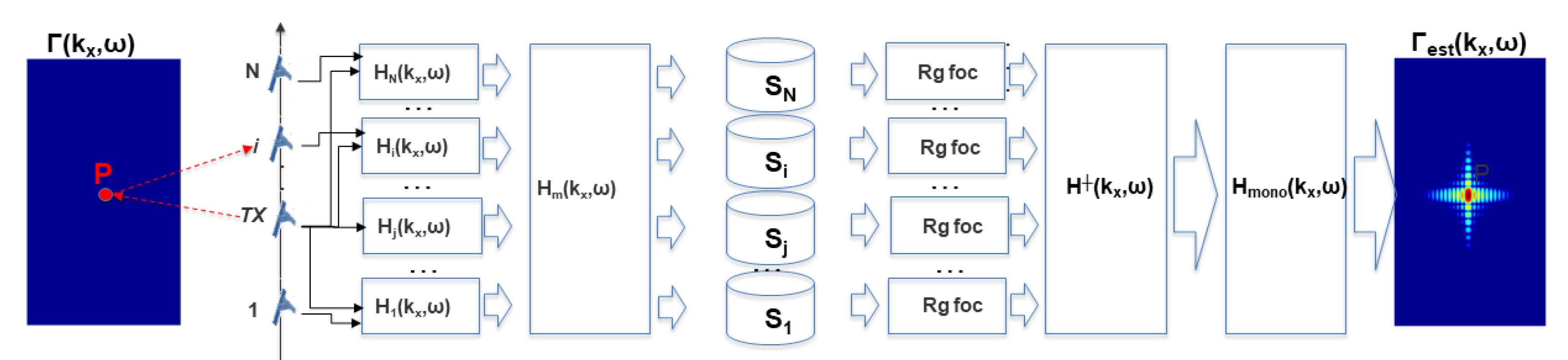
  • A 2D frequency domain spectrum reconstruction method. The effects of noise and bad-conditioned matrix inversion are mitigated by means of a Wiener inversion, similarly to the Minimum Mean Squared Error (MMSE) in [13,14], and considered an optimum compromise between matched and ML filters. The reconstruction in frequency domain is used to account for range migration, as demonstrated also in [16].
  • Two practical methods to mitigate the degradation of system performance due to the loss of position control: a dynamic tuning of PRF and the split of the antenna. Both of the methods that can act together aim at modifying the phase centers towards optimal positions.
  • A systematical study of the degradation in phase shift and volume decorrelation, as a consequence of a realistic non zero across-track baseline, leading to the estimation of a critical tube width for the formation to avoid recombination problems.
Notably, the recombination is invariant with the along the track baseline for typical formations extents (few hundreds of meters), so there is no need to resort to the analysis of residual phase corrections as in [17]. One of the important results in the discussion is that, for formations of satellites irregularly spaced, even with a significant effort to improve the signals recombination with a tunable PRF or displacing the phase centers using the antenna splitting, optimal results in all situations cannot be achieved. For this reason, the efficiency of the recombination is analyzed by resorting to probabilistic considerations, differently from what proposed was in [14,15,18].
The paper is organized as follows: in Section 2, the system is described and the Impulse Response Function (IRF) derived. In Section 3, the recombination algorithm is described. In Section 4, the consequence on system performance of a random positioning of the sensors is analyzed and the methods to mitigate degradation are described and illustrated with simulation results. In Section 5, the effects of a non zero across-track baseline and the possibilities of tomographic formation are discussed. The limits of the system and the conclusions in Section 6 close the paper.

2. SIMO SAR Formation

Let us assume to have N SAR antennas, each put on an independent platform deployed along the track at given positions (known with reasonable accuracy). We also suppose, for now, that all the satellites fly on the same orbit, i.e., the formation has no real-time interferometric or tomographic capabilities. The formation is a Single Input Multiple Output system, one satellite transmits the waveform and each sensor of the formation collects the return backscattered in the common imaged area. The multiple transmitters case (Multiple Input Multiple Output, MIMO) can easily be extended from the model below, but it is beyond the purpose of the study. Initially, we suppose the sensors at a nominal and uniformly spaced distance d x , multiples of 2·PRI apart. In Figure 1, we show the geometry of the formation.

2.1. Design Bounds

System requirements to the formation bring to bound some design parameters.
For a larger swath to be imaged, the Pulse Repetition Frequency (PRF) must be properly lowered to allow the received echoes not to conflict with the transmitted ones. On the other hand, if δ is the output (wanted) azimuth resolution, the Doppler bandwidth must be set accordingly:
B d o p = 0.886 v δ ,
where no distinction has been done between orbital and ground speed v, to avoid confusion (The equations are strictly valid for a rectilinear orbit and flat Earth, but can easily be extended to curvilinear orbit and spherical Earth). The correction factor 0.886 comes from the −3 dB width of a sinc-shaped IRF.
The well-known conflicting requirement for High Resolution and Wide Swath (HRWS) SAR systems comes just from the previous two conditions since a high Doppler bandwidth is possible, without aliasing, only in case of high PRF, which is not the case. However, using the generalized version of the sampling theorem, an aliased Doppler band can still be reconstructed correctly if we have a sufficient number of acquisitions of the same area—in detail, to assure the correct reconstruction, it is necessary that
B d o p R · P R F ,
with R an integer factor describing the ambiguities that must be canceled in the reconstruction, plus one (the ambiguity that is indexed with 0 in the paper is the part of the spectrum to save). Of course, R N , since no more than N ambiguities can be recombined by using N acquisitions.
The PRF is limited below by the achievable azimuth resolution of the monostatic system. In detail, said L a the antenna length, the monostatic azimuth resolution δ m L a / 2 [19]. After reconstruction, we want to improve the azimuth resolution of a factor up to N. For this reason δ = δ m / N . Combining Equation (3) with previous conditions we have:
P R F 2 v N · L a
For the current study this may become a tight inferior bound for PRF since micro- or nano-satellites are not expected to mount long antennas. As an example, in case of micro-satellite of mass 100 kg, a deployable antenna array of L a = 3.5 m is permitted with the current technology, so that with N = 5 satellites and, with v = 7500 m/s, we have P R F 850 Hz.
Finally, an upper bound for the along-track formation extent exists to assure the needed azimuth resolution. The synthetic aperture related to the output resolution δ is:
F S A = v B d o p | F M | = 0.886 2 · λ h δ cos θ ,
where | F M | = 2 v 2 / λ r 0 is the Doppler rate, λ is the wavelength, h is the formation altitude, r 0 a reference slant range, and θ is the incidence angle at r 0 . For a given antenna size, the physical footprint on ground is:
F = λ h L a cos θ .
The maximum extension of the formation is then limited by the condition for all the satellites to look at a common area, at the same time, large at least F S A (see Figure 1b). This means that the inter-satellite distance, in case of equally spaced formation is limited by:
d x F F S A N 1
This bound limits the formation extension and must be evaluated in the orbit control of the system. As an example, for an X-band formation of N = 5 satellites at h = 500 km of altitude, with an incidence angle of 30° and L a = 2 m, if a final resolution of 1 m is required, satellites must be closer than 250 m, which is a safe requirement.

2.2. The Model of the Received Signal

Without loss of generality, let us suppose the formation to illuminate a single point target on ground. We neglect radiometric considerations (i.e., the radar equation and the scattering of the target) and just focus on antenna amplitude and phase response due to the path. Moreover, we neglect synchronization errors between receivers, i.e., the range window alignment among the different response is supposed to be already solved with residual error to be included into a sensitivity analysis (which is beyond the purpose of the paper). The signal transmitted by the master sensor (in the j-th position) bounces on a ground target and is received by each antenna of the formation. After the carrier is removed and the pulse compressed, we have:
h b , i ( t , η ) = A i ( η ) A j ( η ) exp ȷ 2 π λ r i ( η ) + r j ( η ) · sinc B c h 1 c r i ( η ) + r j ( η ) ,
where A i ( η ) and A j ( η ) are the antenna patterns of the i-th receiver and the transmitter, function of the slow time η ; λ is the wavelength; c the light speed, and B c h the chirp bandwidth. r i and r j are the sensor-target distances, function of the slow time and the target position ξ . In case of simple geometry, the slant range distances have a simple formulation:
r i ( η ; ξ ) = r 0 2 + v η d x i ξ 2
and similarly for r j ( η ; ξ ) , with r 0 the minimum approach of the formation center to the target position (We suppose to focus with respect to the formation center, which is also the relative zero for the sensors’ distances and slow time, regardless of the transmitter or any other sensor position.) and d x i the distance of the i-th sensor from the formation center.
In the previous formulation, the rank extent, i.e., the movement of the receiver sensor during the flight of the sequence from transmitter to the target and back to the receiver, has not been considered. It has little effect and shall not be included to avoid useless confusion. The received signals, as expected, are a non separable function of ( t , η ) because SAR impulse response for curved trajectories is range variant.
Likewise, for the traditional monostatic SAR systems, the range migration effect can be efficiently corrected in the two-dimensional wavenumber domain [20], where the convolution of the system function by the target backscattering response is transformed into a multiplication and the reconstruction of the unambiguous spectrum becomes an inversion problem. This is the reason why we perform spectrum reconstruction in a 2D transformed domain.

2.3. The Model in the Frequency Domain

As widely shown in literature [21], representation of the transfer function of a bistatic system is a very hard task. Usually, an equivalent monostatic approximation is adopted for a reasonable distance between the transmitter and receiver. This assumption can be considered valid for a formation extent but not for constellation of satellites [17]. At least, some phase correction can be added in the focusing, as demonstrated in [22].
In the equivalent monostatic approximation and neglecting the antenna terms, the Impulse Response Function (IRF) in Equation (9) can be written as [7]:
h b , i ( t , η ) exp ȷ 4 π λ r 0 · exp ȷ 2 π λ v 2 ( η ( d x i + d x j ) / ( 2 v ) ) 2 r 0 · exp ȷ π 2 λ ( d x i d x j ) 2 r 0 .
In the monochromatic approximation, i.e., when λ c / f c (valid for relative narrow band), the first term is constant w.r.t. η and a function of the minimum formation-target distance; the second term is the phase of an equivalent monostatic SAR [7] delayed of ( d x i + d x j ) / 2 , i.e., halfway between the transmitter and receiver; the third term is a pure bistatic term and it is constant too.
The previous approximation can be adopted to write the 2D signal spectrum in a sampled context. Supposing a backscattering field Γ ( x , r ) acquired by the bistatic sytstem i j (receiver-transmitter couple). The 2D spectrum of the received signal is:
S i ( k x , ω ) = r Γ ( k x + r · k x , s , ω ) · H b , i ( k x + r · k x , s , ω ) ,
where S i ( k x , ω ) is the spectrum of the signal observed by the i-th receiver, k x is the azimuth wavenumber, ω the range pulse, and the repetition in the wavenumber domain k x , s is 2 π · P R F / v .
This signal spectrum is the summation (in principle endless) of the aliased versions of the spectra of the target reflectivity Γ ( k x , ω ) passed through the (aliased) transfer function of the bistatic SAR system. The transfer function of the bistatic SAR is the 2D-Fourier transform of Equation (11):
H b , i ( k x , ω ) = exp ȷ 4 π λ r 0 · F exp ȷ 2 π λ ( v η ) 2 r 0 · exp ȷ k x d x i + d x j 2 · exp ȷ π ( d x i d x j ) 2 2 λ r 0 .
In the previous transfer function, the first two terms correspond to the transfer function of the equivalent monostatic SAR:
H m ( k x , ω ) = exp ȷ 4 π λ r 0 · F exp ȷ 2 π λ ( v η ) 2 r 0 .
The third and fourth terms are specific to the bistatic acquisition:
H i ( k x , ω ) = exp ȷ k x d x i + d x j 2 · exp ȷ π ( d x i d x j ) 2 2 λ r 0 .
A block scheme of the acquisition steps, where bistatic and monostatic acquisition are conceptually divided, and of the corresponding recombination and focusing of the N received signals, is in Figure 2.

3. Reconstruction of the Scene

3.1. Matrix Discrete Formulation

We reformulate the previous equations in a discrete context. A target on ground in position ξ l is acquired by the formation observing the scene for T o b s seconds. M observations are acquired by each receiver, where M = T o b s · P R F . The acquired data can be set in a matrix S collecting the signals acquired by all the receivers whose size is [ N M × P ] with P the number of range samples within a narrow strip in range (We remember that, formally, the SAR impulse response is time variant and the transfer function is different range by range. See Section 3.3).
Using the approximation in Equations (14) and (15), the formulation in Equation (12) can be written in a compact form:
S = H D + N ,
where H (of size [ N M × R ] ) is the (bistatic) combination matrix filled by contributions in Equation (15) and having N · M rows (the number of receivers times the Doppler wavenumber bins) and R columns, with R being the number of frequency sets of width PRF we want to unfold (in principle, infinite, in practice, we can disentangle up to N replicas). The matrix D (of size [ R M × P ] ) is the wavenumber domain support of the signal observed by a monostatic equivalent SAR system. It is the multiplication, element-wise, of two matrices: D = H m Γ , where H m (of size [ R M × P ] ) is a matrix including the contributions of Equation (14), i.e., the equivalent monostatic SAR system put at the center of the formation and Γ (of size [ R M × P ] ) the ground backscattering, both sampled R times denser than each bistatic term, i.e., at nominal positions v / ( R · P R F ) . N is finally the noise matrix.

3.2. Recombination

Reconstruction of the unfolded spectrum of width R · P R F is achieved by minimizing the distance between the true D and the reconstructed D ^ signal, in some norm. In case of white noise added, the 2 -minimization (MMSE in [14]) is performed that corresponds to the pseudo-inverse of H in case of diagonal covariance matrix of data:
D ^ = H S ,
where H = ( H * H ) 1 H * is the Moore–Penrose inverse of matrix H and the apex * means Hermitian (i.e., conjugate of the transpose). Pseudo-inversion may increase the level of noise, especially if the final sampling step is consistently lower than the target resolution since in that case part of the frequency set [ R · P R F / 2 , R · P R F / 2 ] has just noise. For this reason, or when correlated noise is present, the general inversion (also called Wiener inversion) that accounts for data and noise covariance matrices is preferred:
D ^ = H s * S = H C D H * + C N 1 H C D * S ,
with H s = H C D H * + σ n 2 · I 1 H C D and C D and C N the covariance matrix of the acquisition and of noise, respectively.
Estimated inversion, D ^ of size [ R M × P ] is, for each range bin p, the value of the spectrum in the R frequency sets each of width P R F put in positions [ R , , R ] · P R F . Inversion is performed bin-wise for each k x and for a total of M times, to fill the spectrum in the unfolded frequency interval.
The gain of the multistatic formation can be evaluated by estimating the increase of SNR due to recombination. In case of pseudo-inversion, the noise covariance matrix after inversion is:
E H N N * ( H ) * = ( H * H ) 1 C N = σ n 2 · ( H * H ) 1 .
In the last step, we supposed uncorrelated noise and diagonal covariance matrix with power σ n 2 . The signal to noise ratio is then:
S N R = tr C D σ n 2 · tr ( H * H ) 1 .
After some algebra, we achieve the SNR in the general case:
S N R = tr H s * C D H s σ n 2 · tr ( H s * H s ) ,
which of course collapses into Equation (20) in case of the diagonal covariance matrix of the acquired signal C D . Compared to the SNR of the monostatic single sensor, a gain of:
G = 1 tr ( H * H ) 1
is achieved in an ideal condition and the diagonal covariance matrix of the signal. In case of perfect inversion, the gain is N, which is the upper bound for the recombination gain in power and corresponds to what is expected by theory (the signal sums in coherent way, gaining N 2 , the noise in incoherent way, gaining only N) [7].

3.3. Focusing of Equivalent Monostatic SAR

The focusing of the equivalent monostatic system, can be performed with any efficient SAR focusing algorithm. In practice, since, after recombination, data are in the double wavenumber domain, the most easy way to proceed is using a wavenumber focusing method such as the Ω -K algorithm [23]. The wavenumber to build the Ω -K operator is now large 2 π · R · P R F / v and includes R · M bins.
In principle, since SAR impulse response is range-variant, the Ω -K algorithm is exact only at range r 0 and the reconstruction should be repeated for each slant range of the received signal. In practice, anyway, the monochromatic assumption is a good approximation for SAR focusing and a sufficient accuracy can be achieved also by processing narrow slant range strips at a time, using the central range as reference. The width of these strips must be large enough to include the range migration cells of a synthetic aperture for the central target. For LEO orbit SAR, we found that processing few hundreds of range bins produces sufficient accurate results.
A point target focused using N = R = 5 sensor at 500 km of altitude with L a = 3.5 m, PRF = 880 Hz, λ = 0.055 m and formation extent 500 m is shown in Figure 3. Uniform and optimal spacing between sensors has been supposed. As can be seen, the azimuth ambiguities have been reduced to less than −70 dB and, at the same time, the azimuth resolution has been improved to about 2 m. In these optimal conditions, the estimated gain is 13.56 dB, very close to the ideal value 13.98 dB (i.e., 10 log 10 5 2 ).

4. Control of Sensor Position

4.1. Relation between Formation Distance, PRF, and System Performance

Equation (2) provides the conditions for optimal spacing of output samples in a formation, according to a given value of PRF. In case of not uniform output sampling, a degradation of performance is expected as explained in [6,7,8]. In the limit conditions, some output samples coincide, and the corresponding rows of the design matrix H are linearly dependent. In this case, the inversion is not possible unless such rows are discarded, reducing this way the reconstruction capability of the formation to the case R < N .
In SAR design, it is common to select PRF within definite intervals to avoid the returning echoes to collide with nadir returns or with transmitting pulses [19]. The interval of existence of valid PRFs is then a function of the acquisition geometry, in particular of the incidence angles. Once the geometry of acquisition and the swath width is chosen, only some intervals of PRF values are possible. Ideal formation distance must be set according to Equation (2) and such constraint.
In a realistic context, however, the sensor distance cannot be controlled with infinite precision. More commonly, sensors are uniformly set (i.e., nominally in ideal positions, for a given PRF) but, for a uncontrolled extent, δ x that is often modeled as a zero-mean random variable Gaussian distributed with standard deviation of few meters:
d x i = i · d x + δ x .
From Equation (2), it is easy to infer that the minimum distance between a good sensor separation and the next bad separation is as little as N / ( N 1 ) · 2 v / ( N · P R F ) . For a practical system with a PRF under 1000 Hz and N = 5 , this distance amounts to about 3.5 m. It means that the physical separation existing between a good phase center positioning of two consecutive sensors and the closest bad positioning is of the same order of the antenna length. The sensor position in orbit should be controlled within a small fraction of such value, let us say better than 0.3 m. Currently, such a tight control of the sensors position is hardly reachable. Moreover, due to the chaotic behavior of satellites along the orbit, the goal positions, even if reached, could not be guaranteed for a long time, unless the frequent maneuver is adopted, with consequent decreasing of the life span of the mission.
Of course, due to the duality of sensor position and PRF, it is possible to mitigate the degradation due to the loss of the control of sensor position by tuning the PRF.

4.2. Mitigation of System Performance Degradation

PRF tuning to mitigate the effect of system performance degradation due to an unequal sensor position is not a new idea since already investigated in [11] or in [18]. Here, we implement such method in a formation, together with a novel way to further displace the phase centers: the twin antenna concept.
In the next subsections, it shall be clear, however, that mitigation implicitly includes a different definition of quality for random formation of small satellites. In practice, with a small probability, the results may be insufficient for any application. With loose formations, less cost means passing from a deterministic system to a probabilistic one in which performance can be assured within a given degree of reliability. The probability with which any mitigation method may fail is analyzed in Appendix A.
In the following, just two exemplary cases are presented in which the improvement of the performance are shown after the application of the proposed mitigations. In the shown cases, the sensors are in a total random positions. Moreover, the maximum formation extent is fixed, to have a common imaged area large enough to assure the output azimuth resolution. The minimum sensor distance is fixed too, to keep the satellites safe from collisions, let us say three times the standard deviation of the control position plus three times the standard deviation of the knowledge position. According to the current technology, the minimum distance has been set to 30 m.

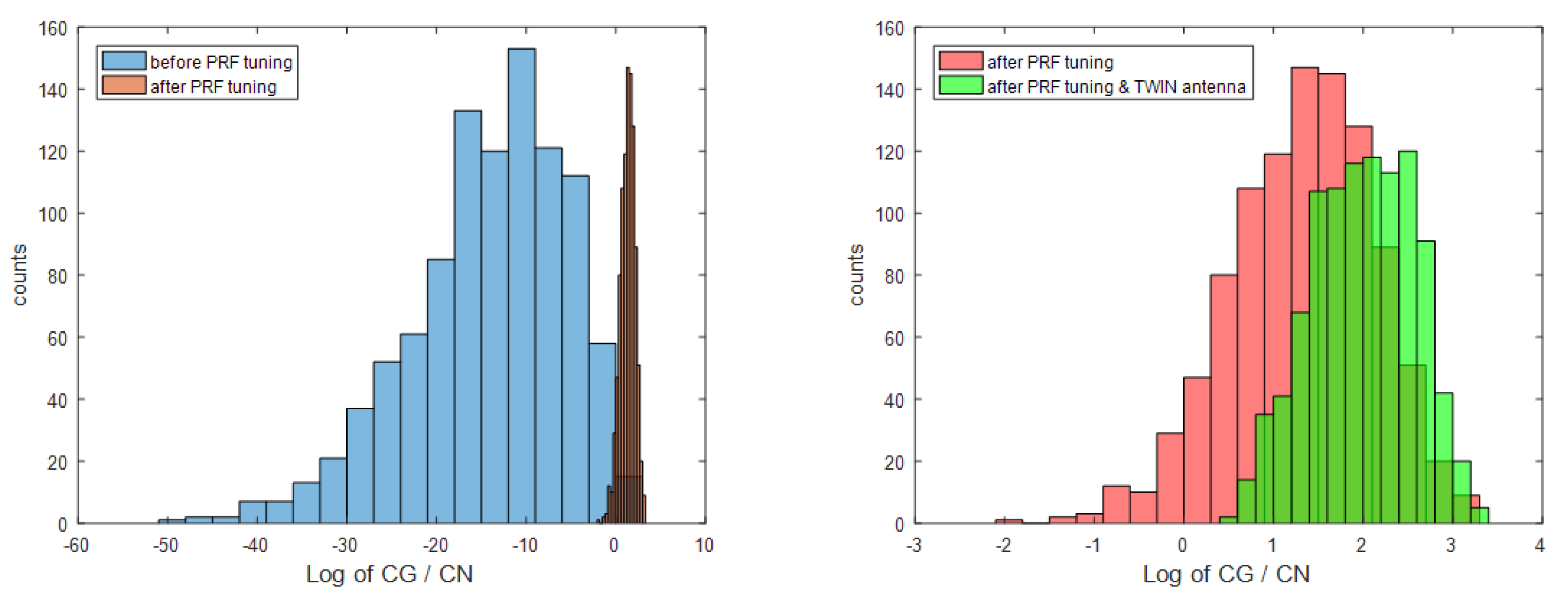
4.2.1. Tuning the PRF
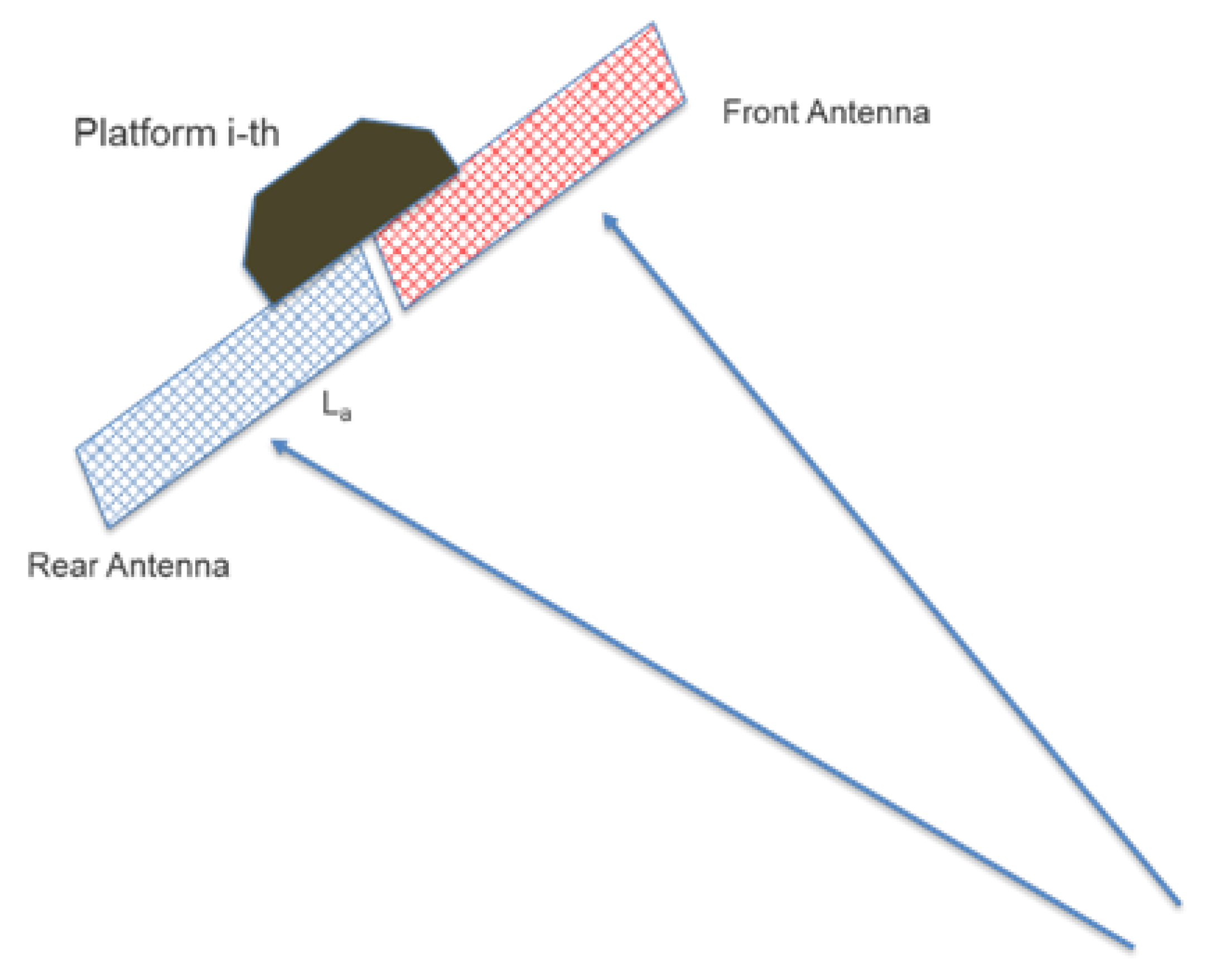
According to Equation (2), the ideal position of sensors even in a not equally spaced formation is given by the choice of proper integers k i , once a PRF is selected. The sensibility of this solution to sensor position is, however, very high: change of the i-th sensor position of δ x implies an adjustment of the corresponding PRF of:
P R F ^ P R F 2 v d x i 2 δ x .
For an LEO orbit, with v = 7500 m/s and a d x i = 50 m, 1 m of uncontrolled shift brings to a PRF adjustment of 6 Hz. This means that the degradation of the formation performance is very sensible to little shifts of a sensor’s position and that PRF must be accurately tuned accordingly. Of course, it may not exist a single value of PRF able to satisfy Equation (2) with integers k i , i = 1 , , N 1 so a sub-optimal PRF must be found in practice.
For a given formation, the true recombination performance is evaluated through the IRF quality (resolution, PSLR, ISLR) and the reduction of azimuth ambiguities. However, it is very difficult to relate such values to the research of a sub-optimal PRF (there is not a simple closed-form expression relating satellite distance, PRF, and performance). For this reason, we adopted an exhaustive research of the optimal PRF according to the quality of recombination, simply measured through the ratio between the recombination gain, given by Equation (22) and the condition number of H * H :
F = 1 tr ( H * H ) 1 · max eig H * H min eig H * H .
The recombination gain is related to the peak gain, the condition number to the quality of the matrix inversion (and so to the reduction of ambiguities). The two quantities are related each other, but they do not express the same thing since the recombination gain is the harmonic mean of the eigenvalues of H * H , while the condition number is the ratio of the maximum and minimum eigenvalues and provides a measure of the matrix conditioning.
The optimization has been applied in a practical case with N = 5, v = 7500 m/s, L a = 3.5 m, λ = 0.055 m, sensor altitude 500 km and d x = [−250 −96.52 20.95 166.55 250] m. The starting value of the figure of performance (the ratio of the reconstruction gain and the condition number), is: 9.2 × 10 7 ( G = −17.64 dB, cond numb = 1.87 × 10 4 ) for a PRF = 880 Hz, so a bad result is expected for ambiguity ratio (PTAR) and IRF main lobe (see Figure 4a,b). After an exhaustive search of the optimum PRF in the frequency set [880,1500] Hz (geometrical constraints have been ignored here), a solution has been found at 1376.33 Hz, for which the figure of performance increased to 3.39 ( G = 12.55 dB, cond numb = 5.31). The corresponding results, shown in Figure 4c,d, are visually better.
The stochastic nature of the mitigation method is better illustrated by evaluating the number of successes achieved through the PRF tuning for many different formation with random sensors’ location. In Figure 5a, the histograms of the figure F before and after the optimization show the wide beneficial effect even when satellites start from purely random position, but that bad cases may still exist and can not be corrected.

4.2.2. Twin Antenna

The second mitigation scheme consists of using a new concept: the twin antenna (see Figure 6). Splitting the antenna consists in using just one half of the antenna as in the multichannel case and, if technologically feasible, enlarging the two halves using some kind of boom.
The twin antenna concept may be exploited in two different ways:
  • Use both rear and front parts, as there were 2 N receivers,
  • Use a proper combination of rear or front that assures the best recombination scheme.
The general principle on which grounds the first possibility is doubling the number of receivers, which is expected to produce beneficial effects as shall be shown in Appendix A. However, it is costly since it requires more satellites or, even in a multichannel case, it generates a doubled data volume. In the second possibility, the use of the front or the rear part of the antenna has a relevant impact on the phase terms in the reconstruction matrix, allowing substantial change in its structure since L a is comparable with the final azimuth resolution. The adoption of a proper combination of the first or of the second halves of the antenna of the various receivers may increase the figure of performance allowing for a better recombination. The advantage with respect to the first solution is to guarantee the same data volume at the cost of reducing to half the total antenna area. This method is expected to produce an improvement in case of displacement of sensors from their optimal positions.
As for the PRF tuning, the pre-computation of the figure of performance for a formation for which we accurately know the sensors location is a feasible task to be done before a programmed acquisition and for all the possible combinations of rear-front of the receivers that are 2 N . The best combination, i.e., the one providing the highest F , is then programmed onboard.
In a practical example, we considered a formation with the same parameters as in Section 4.2.1 but N = 7 and the sensors set in: dx = [−200, −147.776, −91.902, −20.398, 43.245, 115.746, 200] m. In Table 1, the performance of the two mitigation schemes used separately and jointly are compared. As can be seen, although the tuning of PRF produces already acceptable performance (second row), using both the mitigation scheme further improves the recombination gain (i.e., increasing of SNR), despite of half of the antenna area being used and a better reduction of the first azimuth ambiguity and an improved azimuth resolution.
Adoption of a twin antenna further improves the system performance, as shown in Figure 5b, where the figure of performance with PRF tuning only and PRF tuning-twin antenna are compared for a large number of a random positions’ formation.

4.2.3. System Sensibility

As shown in Equation (24), a little change in the PRF may produce large displacement in the phase center locations with a consequent change of the system performance that can be optimized by choosing the best PRF for the current situation. This optimization, however, needs a perfect knowledge of the satellite positions. In the following, we have analyzed the variation of the system performance, increasing the PRF interval values within which the PRF value can be optimized, once given the locations of the satellites. The system performance is measured by the probabilities (in the abscissae) of the losses of SNR (in dB, ordinates).
Figure 7 addresses the probabilities of the losses of SNR for a formation with N = 4 satellites randomly spaced, with a reconstruction multiple equal to R = 2, 3, and 4 (corresponding to the full reconstruction capability). In each figure, the cases with no twin antenna or multiple twin antennas have also been presented. As it can be seen, the case with R = 4 is the most difficult to treat and three out of four possible double antennas are needed to achieve reasonable performances. As an alternative, a larger deviation of the PRF or a larger formation can be used but with more problems of across-track baseline, as to be discussed in the next section.

5. System Limitations

5.1. Across-Track Baseline Effects

For an along-track formation concept, a non zero across-track baseline is an impairment, since even a slight off-track of a sensor provides a received contribution changed by the interferometric phase due to the baseline between the actual and the ideal tracks. This interferometric phase results in a spectral shift and a volumetric decorrelation.
The case of a sensor shifted off-track with respect to the formation, assumed in straight orbit, is shown in the geometry of Figure 8a in the along the track, range reference and in Figure 8b in the reference orthogonal to the orbit. This second figure shows how two or more targets, located in the same iso-range with respect to the non-shifted track (the shaded satellite), contribute with different distances, and then different phases to the shifted sensor imagery. This case resembles an interferometric SAR [24], with the major difference that, in the unfocused images, the number of targets that contribute to the same raw data pixel are spread over a wide azimuth aperture.
This fact is better shown in Figure 9, where it is shown in a rough topography that the effective baseline created by the shift causes a fringe pattern that impacts as a multiplicative phase screen in the raw data. The compensation that requires a precise knowledge of the Digital Elevation Model (DEM) is not easy and may be even not possible.
In the case of a constant sloped terrain, the impact of an off-track shift of the sensor is a spectral shift [25] whose amount depends on the normal baseline, B n , the incidence angle, θ , and the local slope, α :
Δ f = f 0 B n r 0 · tan ( θ α ) .
The impact of the shift can be mitigated by filtering the common spectral contributions: the ones that would be imaged in both on-track and off-track position. The filtering removes any uncorrelated spectral contributions that would act like clutter noise but reduces the total bandwidth by the same amount, Δ f . In a general case, where each sensor has its own shift, the normal baseline B n should be replaced by the total tube, normal to range, in which the formation is kept. For a rough estimation, let us assume the C-band, an incidence angle θ = 30 ° , flat terrain α = 0 and range r 0 = 600 km (reasonable for an altitude of 500 km). If we assume 100 MHz bandwidth, and tolerate a total spectral shift that is 10%—leading to a proportional range resolution loss, we would get an orbital tube:
B n T Δ f f 0 · r 0 · tan ( θ α )
that amounts to about 640 m. This is not so hard requirement to keep, although the presence of a moderate slope of 10 ° would reduce it to 400 m. In the rough topography shown in Figure 9, the compensation should be performed on a local base that in turn would require to implement the SIMO image processing in a back-projection framework. This would possibly solve the problem, although, being the SIMO recombination dependent on wavelength λ , it could be possible, for very large frequency shifts, to get different performance from the combination.
However, the worst case is the one shown in Figure 8b, where multiple targets at different height contribute to the same range with different phase. In fact, even if we were able to perform an adaptive SIMO recombination that integrates a local spectral shift filtering [26], we still would get noise from multiple contributions within a single resolution cell. The impact on the random phase combination that would result can be evaluated in terms of coherence between the ideal data d 0 and the actually acquired one, d B , and relates coherence to SNR:
γ = E d B d 0 * d B d 0 = 1 1 + S N R 1 .
The coherence can be evaluated in terms of the statistics of the target’s height dispersion. For a uniform dispersion in a box of elevation Δ q [24,27], γ = sinc Δ q / q 2 π , where the elevation ambiguity is inversely proportional to baseline:
q 2 π = λ r 0 sin θ 2 B n
Assuming to tolerate a slight signal to noise ratio degradation, we can approximate Equation (28):
γ 1 S N R 1 1 π 2 6 Δ q q 2 π q 2 π 1.6 · S N R · Δ q .
This means that, if we assume a dispersion of target in a box of Δ q = 50 m, like, for rough topography, mostly urban, and we tolerate an SNR no worse than 10 dB, the elevation of ambiguity should be q 2 π > 4 Δ q = 200 m. In turn, the maximum offset normal to range should not exceed B n = 40 m. This is indeed the most stringent requirement to be fulfilled.
If the across track baselines of the satellites are supposed to be perfectly known, the unique unknown affecting the cancellation of the R ambiguities is the height of the target. The phases with which the target contributes to the R ambiguities are also related to the baselines.
In order to approximately evaluate this effect, let us consider the decrease of ambiguity cancellation when the height error q h is very small, so that it is possible to linearize. Then, instead of the perfect closure of the phases that would allow for annihilate the interfering ambiguity, a noise component is added to the data. We can briefly approximate the impact of the dispersion of the cross-track baselines on the ambiguity suppression AASR. To do so, we will suppose that the azimuth ambiguity has already been canceled and the receivers are exactly at their optimal positions, so that we will consider only the impact of the cross-track baselines. In this case, the residual ambiguity affecting another pixel at the ambiguity distance will be:
y = x N n = 1 N exp j 2 π n N + j 2 π Δ q H n ,
where Δ q is the height error, N is the number of the receiving satellites with returns to be combined to remove the ambiguity, x is the local reflectivity, and Q n :
Q n = r λ sin θ 2 B n
are the altitudes of ambiguity of the n = 1 ,   ,   N satellites, with positive and negative cross track baselines B n , θ is the incidence angle, r is the distance.
Obviously, if Δ q is zero, the ambiguity is canceled. However, just supposing Δ q small and linearizing it, we have
y = j x 4 π Δ q N r λ sin θ n = 1 N B n .
Representing with σ h the dispersion of the height error, the total power of the ambiguity is:
R · E y 2 = R · x 2 4 π σ h N r λ sin θ 2 N σ β 2
as there are R ambiguities to be removed.
Hence, we have:
A A S R = 4 π r λ sin θ 2 R N σ h 2 σ β 2 .
Considering as an example, L band, r = 600 km, N = 4 , R = 3 , θ = 30 ° , we have:
A A S R = 4 π 600000 0.24 0.5 2 3 4 σ h 2 σ β 2 = 2.28 × 10 8 σ h 2 σ β 2 .
If we wish to keep the AASR better than 20 dB:
σ h σ β < 0.01 2.28 × 10 8 = 662 .
If σ h = 10 m, then σ b < 66 m that appears to be indeed very difficult unless we mitigate the effect recurring to autofocus methodologies to unmix, as to be briefly discussed in the following.
If the DEM has lower resolution, then the number of unknown heights would decrease and one could try to estimate them with unmixing but still, as common to all unmixing problems [22,28], any solution would be acceptable unless the higher order moments of the amplitude statistics are used. Furthermore, in the case of full resolution, two degrees of freedom only (the real and imaginary part of the reflectivity) are available for each unknown (the height error) and thus hardly sufficient for any reliable estimate of the height. For lower and lower resolution of the DEM (say just a slope), a solution might be found but only in the case of a very active texture of the data. The obvious cure is to keep q high, the cross track baselines small and thus the formation short. However, then, if the positions of the satellites are random and the adaptation of the PRF becomes insufficient, the additional antennas become mandatory to reduce the ambiguities. For small height errors, hypothetically, an autofocusing code could be considered that maximize the contrast in each one of the R affected positions by modifying the height of the contributing target. However, then, the targets in the affected positions would already be disturbed by the other R 1 ambiguities. The solution would only be obtained with a code that considers M points mutually ambiguous and thus distanced of a footprint, and finds their M heights by maximizing the M contrasts and /or their reciprocal independence. It is not impossible that such a code could work, but indeed highly unlikely, also because the maximum contrast need not to be the correct solution. Furthermore, in the case of targets with Gaussian distributions with the same variance, the unmixing would be utterly impossible. Still, as said, things get easier and maybe doable if the DEM is lowpass.

5.2. Tomographic Formations

The previous analysis indicates that the main difficulty for using loose formations for a proficient SAR design comes from the narrowness of the orbital tube needed, as seen in the previous section. Indeed, lower frequency bands like S or L would lead to lesser prerequisites, but then the dimensions of the antennas would grow making less likely the hypothesis of nanosatellites. Still, the selection of S band for the nanosatellites CIRES [29] indicates that these solutions should not be discarded at all.
Then, one could extremize the message coming from the previous considerations, and hint that formations of small satellites could best fit for tomographic applications, i.e., enhancing the role of the unwanted across track baseline, rather than reducing it at most. In other words, an interesting application for these formations could be derived from the availability of simultaneous multi-baseline data that would substantially abate the temporal decorrelation effects. In this view, the formation could be used for another purpose, renouncing to the extended swath and improved resolution, and exploiting the multeplicity of the satellites to analyze a layered medium, provided that the frequency used allows that penetration. Supposing that N receivers are available, N H N layered medium could be studied.
Let the across track baseline be B i j , and D i j the distance between the midpoint of the transmitter j and the receiver i and the formation center and with x h , H h the complex amplitude of the return and the height of the h t h layer. n i j is the noise. The returns are
y i j = i . j , h x h exp j 4 π λ B i , j H h R sin θ + j k D i j 2 + n i j .
The model matrix A is:
Y = y 1 y N ; X = x 1 x N H A = N × N H ; Y = A X + N , a i , j , h = m exp j 4 π λ B i , j H h R sin θ + k D i j 2 ,
A = m exp j 4 π λ B m , 1 H 1 R sin θ + k D m 1 2 m exp j 4 π λ B m , 1 H N H R sin θ + k D m 1 2 m exp j 4 π λ B m , N H 1 R sin θ + k D m N 2 m exp j 4 π λ B m , N H N H R sin θ + k D m N 2 .
The eigenvalues of the matrix A with a random distribution of the B’s and D’s are shown in Figure 10 in an example where the diameter of the formation is between 100 and 1000 m, H max = 50 m and N H = 4. We see that we have good conditioning as soon as the diameter is beyond 700 m.

6. Conclusions

Loose formations of small satellites open new paths towards higher performances allowing major scalability, less exposure to single point failure and reduced costs. In this paper, it has been shown that along the track formation of small satellites, even loosely controlled in their position, can provide high resolution and SNR, wide swath coverage, and good ambiguity suppression. Simulations have been used to demonstrate the goodness of the recombination and mitigation methods since, currently, data from formations of mini-satellites are not available yet. To show results on real data, it would need to make modification of real datasets, in order to emulate the acquisition by the different viewpoints of a formation. This requires a very detailed software simulator and will be a matter of successive work.
Degradation of performance when sensors lose their optimal position along the track has been analyzed also from a probabilistic point of view. PRF tuning, especially when combined with antenna splitting, have been shown to offer superior performance, avoiding a too frequent control of the sensors’ position in order to increase the operative lifetime of the mission. Anyway, for few configuration cases and longer formation extents, the mitigation methods may not guarantee a sufficient recover of the performances.
It appears that formations are better fit for lower frequencies, whereas, for higher frequencies, constellations of small independent satellites would be simpler to adopt. In fact, the ambiguities suppression necessary for a wider swath that would motivate the formation is limited by the very narrow orbital tube needed. In this view and according to the needs, the same formation may be alternatively used for one-pass tomographic applications exploiting the non-zero across-track baseline. A phase term correction, derived from a possible autofocus method, could be considered as a mitigation scheme to counteract the baselines effect. This topic may be a matter of future investigation.
We finally remark that, since such formations are stochastic in nature, design them to achieve always predictable and optimal results would lead to costs likely higher than those encountered with large satellites, contradicting the initial motivations. Rather, these systems are adaptive in nature, yielding quite interesting results, but never guaranteeing perfection and working at all times. The definition of quality of SAR images could be revised to explore costs and benefits of these stochastic solutions. The next step should be a thorough analysis of the propulsion technologies to be used that indeed could determine the possibilities and the limits of this concept, now ready to be explored in practice.

7. Patents

The concepts of multistatic MIMO SAR for formation of small satellites and the twin antenna are currently (15 November 2019) under patent evaluation.

Author Contributions

Conceptualization: P.G., A.M.G., and F.R.; Methodology: P.G. and A.M.G.; software: P.G.; Validation: P.G. and D.G.; writing: P.G., A.M.G., and F.R.; editing and supervision: A.M.G., D.G., and N.G. All authors have read and agreed to the published version of the manuscript.

Funding

This research was funded by European Space Agency, under the Earth Observation Program: # EOP- Φ MM/2018-01-2060/NG/ng.

Acknowledgments

The work has been carried out in the framework of an ESA Earth Observation Program. The authors are deeply indebted to the anonymous reviewers who contributed to the improvement of the paper.

Conflicts of Interest

The authors declare no conflict of interest.

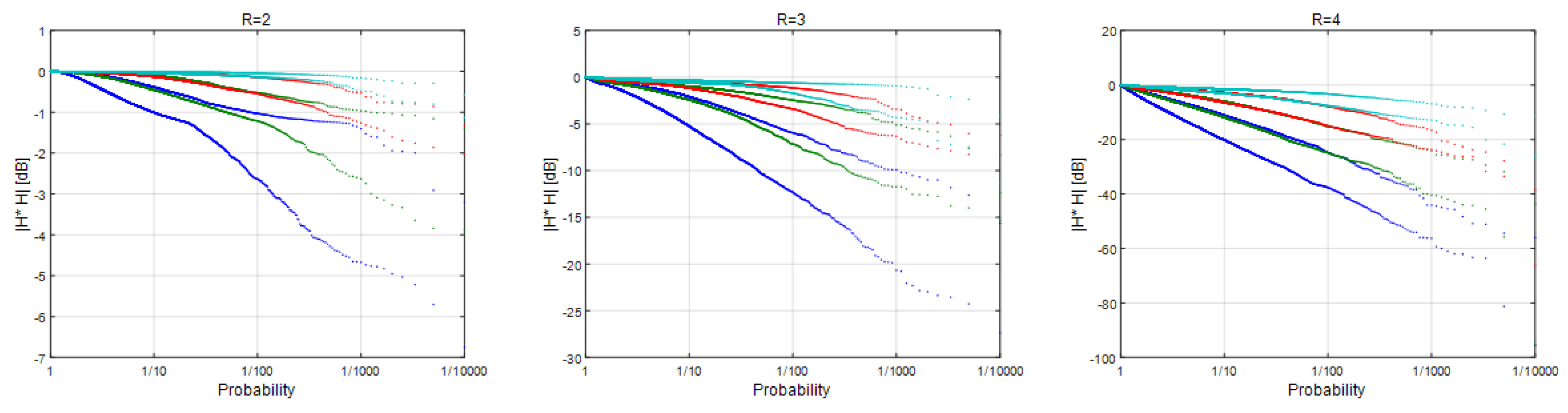
Appendix A. Probabilistic Approach to Matrix Inversion

In Section 4, it has been shown that a SAR formation with a random distribution of sensors position may yield insufficient results. For this reason, a different definition of quality can be proposed, dependent on the application. Optical sensors are limited by night and clouds, and are accepted with their drawbacks. HRWS SAR formations are closer to optical systems, in some way. The additional costs of the methodologies that have been proposed to compensate for the uneven distribution of the sensors, i.e., adaptive PRF and/or twin antenna, may or may not balance the improvements in the probability of correct reception, depending on the available technology. The calculation of the probabilities of failure becomes then a necessary step.
Let us rewrite the recombination matrix H in Equation (14) normalizing the midpoint corresponding to the equivalent monostatic position between the transmitter and a receiver i, i.e., ( d x i + d x j ) / 2 , by relating it to the ground resolution of the current PRF, δ m :
( d x i + d x j ) / 2 = μ i · δ m .
Since the on board antenna is shorter than 2 δ m , R 1 ambiguities will appear in the focused image, positioned at locations indexed by r:
ξ r = ξ + r λ r 0 2 δ m .
The corresponding backscattered radiation, within the monostatic approximation, will rotate by r (the ambiguity index) cycles in the interval δ m . Previously, ξ is the position of the illuminated target and r 0 its slant range. The signal backscattered from the position ξ has phase:
ϕ = ξ 4 π λ δ m μ i 2 r 0 = π ξ μ i F ,
with F given by Equation (7).
The r-th aliased phase will be then:
ϕ r = ξ + r F 4 π δ m μ i 2 λ R 0 = ξ F + r π μ i .
Using the simplified form in Equation (A2) and posing ξ / F = q , the recombination matrix is a Vandermonde matrix, similarly to what already achieved in [15]:
H = exp j μ 1 q exp j π μ 1 R 1 + q exp j π μ N q exp j π μ N R 1 + q .
For a purely random position of the receivers, this matrix assumes the form of a total random complex matrix whose behavior in terms of inversion, can be described by the Marchenko–Pastur theory [30]. There, the probability density function of the distribution of the eigenvalues of H * H is limited in an interval that is a function of the ratio between the number of rows divided by the number of columns. In Figure A1, there is an example of such distribution for different ratios. As shown in the figure, to limit the condition number of H * H to 10 dB (a reasonable value for the matrix conditioning), it is necessary this ratio to be at least 3. In a contrary case, the probability that the inversion is bad-conditioned becomes significant.
This fact leads the project towards a number of satellites N (the number of matrix rows) considerably higher than the number of ambiguities to remove, R (the number of the matrix columns). In the example of Section 3.3, in case of purely random position, to get a reconstruction of similar quality of Figure 3 with R = 4 , it would have been necessary to increase the number of satellites to three times as least, i.e., N = 12. The mitigation methods proposed in Section 4 mitigate the performance degradation saving at the same time resources, since displacing the phase center by PRF tuning or by twin antenna may be as effective as increasing the number of satellites.
Figure A1. Probability Density Function of the eigenvalue distribution for matrix H * H . The different curves refer to the ratio between the number of rows divided by the number of columns. The case 0.5 cannot occur and it is put just as reference, since in this case replicas could not be solved.
Remotesensing 12 00124 g0a1
In practical formations, it is possible to visualize the direct effect of a bad conditioning by looking at the increment of the ambiguity level. In Figure A2, a cube is shown corresponding to the distribution of the positions, relative to the transmitter, of three other receivers (the case N = 4 is then shown). All the points in the cube have the same probability to occur in order to explore the full space of random positions among the four satellites. The optimal positions of the receivers are indicated with black spheres. There are six, corresponding to the six permutations of the receivers in the positions δ m / 4 ; δ m / 2 ; 3 δ m / 4 . The surface identifying the part of the volume of the cube where the determinant of the matrix H * H is between the maximum and −10 dB below (which is just an indicative bound for the ambiguity increasing) is indicated with cyano ( R = 4 ), light-orange ( R = 3), or red ( R = 2) isosurfaces. The probability of a good conditioning is acceptable only for R = 2 , i.e., when the reconstructed replicas are consistently lower than the number of sensors. In practice, the figure visually provides a way to evaluate the precision needed for the positioning, which is approximately 10% of the sampling interval. From the figure, it is possible to appreciate the advantages that can be obtained by letting the antennas to slide along the orbit, or equivalently changing the sampling interval, namely adapting the PRF to the actual positions of the sensors.
Figure A2. Isosurfaces of the value of the determinant of H * H at −10 dB with respect to its maximum value. The case N = 4 satellites with the transmitter as a reference and the remaining three free to move in the space [ 0 , δ m ] × [ 0 , δ m ] × [ 0 , δ m ] has been considered. The black spheres are the in location where the maximum of the determinant is achieved; the isosurface in cyano, light-orange, and red correspond to the R = 4 , R = 3 , R = 2 cases, respectively.
Remotesensing 12 00124 g0a2

References

  1. What is Space 4.0? Available online: http://www.esa.int/About_Us/Ministerial_Council_2016/What_is_space_4.0 (accessed on 28 December 2019).
  2. Yuen, B.; Sima, M. Low Cost Radiation Hardened Software and Hardware Implementation for CubeSats. Arb. Rev. 2018, 9, 46–62. [Google Scholar] [CrossRef]
  3. Currie, A.; Brown, M.A. Wide-swath SAR. IEE Proc. F-Radar Signal Process. 1992, 139, 122–135. [Google Scholar] [CrossRef]
  4. Younis, M.; Fischer, C.; Wiesbeck, W. Digital Beamforming in SAR Systems. Geosci. Remote Sens. IEEE Trans. 2003, 41, 1735–1739. [Google Scholar] [CrossRef]
  5. Mittermayer, J.; Runge, H. Conceptual studies for exploiting the TerraSAR-X dual receiving antenna. Geosci. Remote Sens. Symp. 2003, 3, 2140–2142. [Google Scholar]
  6. Krieger, G.; Gebert, N.; Moreira, A. Unambiguous SAR Signal Reconstruction from Nonuniform Displaced Phase Center Sampling. Geosci. Remote Sens. Lett. IEEE 2004, 1, 260–264. [Google Scholar] [CrossRef] [Green Version]
  7. Gebert, N.; Krieger, G.; Moreira, A. Digital Beamforming on Receive: Techniques and Optimization Strategies for High-Resolution Wide-Swath SAR Imaging. IEEE Trans. Aerosp. Electron. Syst. 2009, 45, 564–592. [Google Scholar] [CrossRef] [Green Version]
  8. Gebert, N.; Krieger, G.; Moreira, A. Multichannel Azimuth Processing in ScanSAR and TOPS Mode Operation. Geosci. Remote Sens. IEEE Trans. 2010, 48, 2994–2998. [Google Scholar] [CrossRef] [Green Version]
  9. Aguttes, J.P. The SAR train concept: Required antenna area distributed over N smaller satellites, increase of performance by N. In Proceedings of the IGARSS 2003, 2003 IEEE International Geoscience and Remote Sensing Symposium, Toulouse, France, 21–25 July 2003; IEEE Cat. No.03CH37477. Volume 1, pp. 542–544. [Google Scholar] [CrossRef]
  10. Burns, R.; McLaughlin, C.A.; Leitner, J.; Martin, M. TechSat 21: Formation design, control, and simulation. In Proceedings of the 2000 IEEE Aerospace Conference, Big Sky, MT, USA, 25 March 2000; (Cat. No.00TH8484). Volume 7, pp. 19–25. [Google Scholar] [CrossRef]
  11. Cerutti-Maori, D.; Sikaneta, I.; Klare, J.; Gierull, C.H. MIMO SAR Processing for Multichannel High-Resolution Wide-Swath Radars. IEEE Trans. Geosci. Remote Sens. 2014, 52, 5034–5055. [Google Scholar] [CrossRef]
  12. Li, Z.; Wang, H.; Su, T.; Bao, Z. Generation of wide-swath and high-resolution SAR images from multichannel small spaceborne SAR systems. IEEE Geosci. Remote Sens. Lett. 2005, 2, 82–86. [Google Scholar] [CrossRef]
  13. Sikaneta, I.; Gierull, C.H.; Cerutti-Maori, D. Optimum Signal Processing for Multichannel SAR: With Application to High-Resolution Wide-Swath Imaging. IEEE Trans. Geosci. Remote Sens. 2014, 52, 6095–6109. [Google Scholar] [CrossRef]
  14. Goodman, N.; Sih Chung, L.; Rajakrishna, D.; Stiles, J. Processing of Multiple-Receiver Spaceborne Arrays for Wide-Area SAR. Geosci. Remote Sens. IEEE Trans. 2002, 40, 841–852. [Google Scholar] [CrossRef]
  15. Cheng, P.; Wan, J.; Xin, Q.; Wang, Z.; He, M.; Nian, Y. An Improved Azimuth Reconstruction Method for Multichannel SAR Using Vandermonde Matrix. IEEE Geosci. Remote Sens. Lett. 2017, 14, 67–71. [Google Scholar] [CrossRef]
  16. Cerutti-Maori, D.; Klare, J.; Sikaneta, I.; Gierull, C. Signal Reconstruction with Range Migration Correction for High-Resolution Wide-Swath SAR Systems. In Proceedings of the 10th European Conference on Synthetic Aperture Radar, EUSAR 2014, Berlin, Germany, 3–5 June 2014; pp. 1–4. [Google Scholar]
  17. Sakar, N.; Rodriguez-Cassola, M.; Prats-Iraola, P.; Reigber, A.; Moreira, A. Analysis of Geometrical Approximations in Signal Reconstruction Methods for Multistatic SAR Constellations with Large Along-Track Baseline. IEEE Geosci. Remote Sens. Lett. 2018, 15, 892–896. [Google Scholar] [CrossRef]
  18. Krieger, G.; Gebert, N.; Moreira, A. SAR signal reconstruction from non-uniform displaced phase centre sampling. In Proceedings of the 2004 IEEE International Geoscience and Remote Sensing Symposium, IGARSS 2004, Anchorage, AK, USA, 20–24 September 2004; Volume 3, pp. 1763–1766. [Google Scholar] [CrossRef] [Green Version]
  19. McDonough, R.N. Synthetic Aperture Radar: Systems and Signal Processing; Wiley Series in Remote Sensing; Wiley-Interscience: Hoboken, NJ, USA, 1991. [Google Scholar]
  20. D’Aria, D.; Monti Guarnieri, A. High-Resolution Spaceborne SAR Focusing by SVD-Stolt. IEEE Geosci. Remote Sens. Lett. 2007, 4, 639–643. [Google Scholar] [CrossRef] [Green Version]
  21. D’Aria, D.; Guarnieri, A.M.; Rocca, F. Focusing bistatic synthetic aperture radar using dip move out. IEEE Trans. Geosci. Remote Sens. 2004, 42, 1362–1376. [Google Scholar] [CrossRef]
  22. Kraus, T.; Krieger, G.; Gerhard, K.; Moreira, A.; Bachmann, M. Addressing the Terrain Topography in Distributed SAR Imaging. In Proceedings of the IET International Conference on Radar Systems (Radar), Toulon, France, 23–27 September 2019. [Google Scholar]
  23. Bamler, R. A comparison of range-Doppler and wavenumber domain SAR focusing algorithms. IEEE Trans. Geosci. Remote Sens. 1992, 30, 706–713. [Google Scholar] [CrossRef]
  24. Ferretti, A.; Monti Guarnieri, A.; Prati, C.; Rocca, F.; Massonnet, D. SAR Principles: Guidelines for SAR Interferometry Processing and Interpretation; Technical Report; ESA: Paris, France, 2017. [Google Scholar]
  25. Gatelli, F.; Monti Guamieri, A.; Parizzi, F.; Pasquali, P.; Prati, C.; Rocca, F. The wavenumber shift in SAR interferometry. IEEE Trans. Geosci. Remote Sens. 1994, 32, 855–865. [Google Scholar] [CrossRef] [Green Version]
  26. Fornaro, G.; Guarnieri, A.M. Minimum mean square error space-varying filtering of interferometric SAR data. IEEE Trans. Geosci. Remote Sens. 2002, 40, 11–21. [Google Scholar] [CrossRef]
  27. Bamler, R.; Just, D. Phase statistics and decorrelation in SAR interferograms. In Proceedings of the IGARSS ’93-IEEE International Geoscience and Remote Sensing Symposium, Tokyo, Japan, 18–21 August 1993; Volume 3, pp. 980–984. [Google Scholar] [CrossRef]
  28. Comon, P.; Jutten, C. Handbook of Blind Source Separation; Academic Press: Cambridge, MA, USA, 2010. [Google Scholar]
  29. Peral, E.; Wye, L.; Lee, S.; Tanelli, S.; Rahmat-Samii, Y.; Horst, S.; Hoffman, J.; Yun, S.; Imken, T.; Hawkins, D. Radar Technologies for Earth Remote Sensing From CubeSat Platforms. Proc. IEEE 2018, 106, 404–418. [Google Scholar] [CrossRef]
  30. Marchenko, V.A.; Pastur, L.A. Distribution of eigenvalues for some sets of random matrices. Mat. Sb. (N.S.) 1967, 72, 507–536. [Google Scholar]
Figure 1. (a) the concept scheme. r i , k and r j , k are achieved in Equation (10) by simple geometric considerations; (b) a simplified view of the acquisition on a common area. In orange, the antenna pattern; in blue the common area imaged by all the sensors (details are in Section 2.1).
Remotesensing 12 00124 g001
Figure 2. End-to-end model of the acquisition (left part) and focusing (right part). Bistatic transfer functions H i ( k x , ω ) are specific of each tx-rx couple; the monostatic transfer function H m ( k x , ω ) is common. The S i are the different raw received signals. After range compression, focusing consists of: (i) inversion of the recombination matrix (see Section 3.2), (ii) traditional SAR focusing at full azimuth sampling step (see Section 3.3).
Remotesensing 12 00124 g002
Figure 3. Focused IRF of a point target for N = R = 5 and uniform spacing of sensors. Left: 2D IRF power; center: azimuth cut at maximum range sample; right: interpolated main lobe.
Remotesensing 12 00124 g003
Figure 4. Focused IRF of a point target for N = R = 5 and sensors in random position. (a,c) Along-track cut of the focused IRF; (b,d) oversampling of the 2D focused IRF. Case (a,b): figure of performance 9.2 × 10 7 ; case; (c,d): figure of performance 3.39.
Remotesensing 12 00124 g004
Figure 5. Histogram of the logarithm of the figure of performance for different random positioning of the sensors in a formation of 400 m of extent, N = R = 5 and parameters as above. (Left) log F before (blue) and after (red) the PRF tuning. (right) log F with PRF tuning only (red) and with PRF and twin antenna optimization (green). Low values address a bad reconstruction.
Remotesensing 12 00124 g005
Figure 6. Concept scheme of the twin antenna.
Remotesensing 12 00124 g006
Figure 7. The probability that 10 log 10 | H * H | is lower than the ordinate is shown for N = 4, and R = 2 (left), R = 3 (center), R = 4 (right). The color of the dots indicates the number of antenna pairs: blue (none), green (one), red (two), cyan (three). The two graphs of the same color correspond to the two different PRF intervals considered, equivalent to adding one or three sample intervals in the full length of the formation.
Remotesensing 12 00124 g007
Figure 8. Geometry illustrating the off-track shift of a sensor in the formation in the along the track, range (a) and elevation, range (b) references.
Remotesensing 12 00124 g008
Figure 9. Impact of an off-track shift of the sensor on the raw data, in the presence of surface topography. (a) geometry, notice the wide azimuth antenna aperture represented in orange line; (b) topographic phase screen that is superposed to raw data. The green band defines a range resolution cell.
Remotesensing 12 00124 g009
Figure 10. Eigenvalues of A (in dB) for a tube diameter from 100 to 1000 m, with an H m a x = 50 m and N H = 4. Little tubes have the greatest dynamics between minimum and maximum eigenvalues.
Remotesensing 12 00124 g010
Table 1. Comparison of IRF performance parameters after recombination using different mitigation schemes.
OptimizPRF [Hz]Cond NumbGain [dB]Peak Power [dB]1s Ambig [dB]Az Resol [m]PSLR [dB]2D ISLR [dB]
N o n e 65077.9410.6316.051.301.882−17.81−9.47
P R F o p t 1337.6249.4611.4014.48−58.331.321−36.21−10.02
T w i n o p t 6501.9314.2415.57−27.611.778−16.46−9.03
B o t h o p t 1337.624.1915.0213.44−69.521.118−30.42−10.14

