Simulation Study of Moon-Based InSAR Observation for Solid Earth Tides

Abstract

The observation of solid earth tides (SET) provides an important basis for understanding the structure of the earth’s interior, and has long been the focus of research in geoscience. However, actually, there still exist some limitations in capturing its global-scale information only with ground stations. Remote sensing technology can realize large-scale deformation monitoring of high point density constantly. However, it is still difficult for the artificial satellite system to meet the requirements of SET monitoring in terms of field of view and temporal resolution now. In this work, the moon is hypothesized as a new platform for SET observation combined with interferometric synthetic aperture radar (InSAR) technology. Based on the tidal model and lunar ephemeris, the spatial and temporal characteristics of the SET from the lunar view were analyzed. Furthermore, the calculations demonstrate that more abundant SET information can be observed in this view. After comparing various observation modes, the single-station with repeat-pass differential InSAR was selected for this simulation. We mainly considered the restriction of observation geometry on moon-based InSAR under three signal bandwidths, thereby providing a reference for the sensor design. The results demonstrate that the moon-based platform offers the potential to become an optimal SET observation method.

1. Introduction

The solid earth tides (SET) is a global phenomenon which reflects periodic deformation of the earth’s interior and surface caused by the gravitation of the sun, moon, and other celestial bodies. It can cause radial undulations of 50 cm in low latitudes [1]. As an important interdisciplinary subject connecting astronomy, geodesy, and geophysics, the SET holds significant research value. There are many methods to calculate the tide-generating potential (TGP), and it can be used to predict the site displacement caused by the SET combined with the theoretical parameters of the earth’s internal medium, such as density, lame parameter, and Love number. Similarly, provided that the earth’s surface displacement can be observed with sufficient precision, the complex information on the earth’s internal medium can also be obtained. The observation of the SET is conducive to the study of the earth’s internal physical structure, which can further promote the development of geophysics [2].

The development of observation methods for the SET has included the tidal gauge, the horizontal pendulum, the gravimeter, and the strain gauge. Among them, the superconducting gravimeter has become an internationally recognized instrument with the highest accuracy, continuity, and stability [3]. However, these measurement methods show some inherent limitations. For example, they can only obtain tidal information at stations, which means that very dense ground stations are needed if we want to get global-scale information. This will consume a large amount of ground resources. Furthermore, the observation environments and conditions of different stations vary significantly, causing the observed tidal parameters to contain strong local environmental factors [4]. Therefore, it is difficult to capture the overall changes of the SET. If a large-scale surface deformation observation method was available, the distribution information of the earth’s internal attributes could be acquired. Moreover, if this observation method had a sufficient temporal resolution, the change of the earth’s interior could be monitored in real time.

The development and application of space geodesy technology have brought new possibilities for the observation of SET. Some space technologies such as very long baseline interferometry (VLBI), global positioning system (GPS), lunar laser ranging (LLR), and satellite laser ranging (SLR), have contributed to the observation of SET. For example, GPS technology is used to correct the asymmetric atmospheric residuals in the observation of gravity solid tides [5]. However, it is still difficult to directly observe the SET displacement through GPS networks. There is a need to improve the sampling density of GPS networks. The special texture features of displacement distribution can be easily hidden in various errors. Furthermore, in any geodetic analysis, it is important to consider how the displacement of SET may affect the instantaneous site position, and it is mainly through the SET model or the assumption that the average values of the unmodeled periodic ground displacement with approximate semidiurnal and diurnal periods are close to zero. [6,7]. This means that high-precision geodesy needs the theoretical displacement of SET. It is hard to distinguish the difference between the actual displacement and the theoretical displacement of SET from other types of surface displacement without combining the special texture information.

Interferometric synthetic aperture radar (InSAR) is a space technology that has been rapidly developed in recent years. InSAR extracts phase information from the complex radar data of the synthetic aperture radar (SAR). It also conducts interference processing to determine the three-dimensional (3D) information of the earth’s surface accurately [8], and effectively captures large areas of deformation [9]. This technique can be successfully applied to topographic surveys, seismic deformation measurements, land subsidence, volcano monitoring, landslide monitoring, and land cover applications [10,11,12,13,14,15]. Numerous research results have evidenced that the accuracy of the differential InSAR (D-InSAR) technique in measuring surface deformation, such as earthquakes, ground subsidence, and landslides, can reach or exceed centimeters [16,17,18,19,20]. Therefore, InSAR technology offers significant potential in the study of geodynamics. Compared to other space ranging methods, such as global navigation satellite system (GNSS), VLBI, and SLR, InSAR technology exhibits better deformation monitoring accuracy, spatial continuity, and point sampling density. More importantly, it is not limited by the number of ground stations [21]. These features of InSAR make it feasible to retain spatial texture, which is beneficial for SET observation. Of course, it also has some drawbacks in some applications, such as in crustal movements that occur over large areas. This is because it is difficult for the InSAR to recognize constant movements involving ground reference points, and its shortest monitoring interval is for a revisit period. Furthermore, atmospheric disturbances and phase decorrelation may have prevented this technique from achieving its full operational capability. We can carry out measurements on a subset of image pixels corresponding to permanent scatterers (PS) and make use of long temporal series of interferometric data to overcome these drawbacks. Moreover, the PS information can be compared and calibrated with other kinds of information such as the GNSS network. Great progress has been made in the development of a more detailed surface motion map by merging GNSS information with SAR datasets [22,23].

According to the theoretical displacement distribution characteristics of SET (usually with a gradient of less than 1 cm/100 km for vertical displacement and less than 2 mm/100 km for horizontal displacement, as shown in Figure 2), the deformation gradient in the field of view (FOV) is rather insignificant for low-orbit SAR satellite platforms. This is not only because of the limitation in the orbit height, but also the operation mode of the artificial satellite, which makes it hard to observe the significant displacement region of the SET most of the time. In addition, they have long revisit periods and the state of SET is constantly changing, which makes the SET information between adjacent swaths totally different. Given this, it is difficult to achieve the spatial continuity and temporal consistency required by global-scale SET observation. The inclined geosynchronous orbit satellite SAR has an orbital altitude of 36,000 km, and has essentially met the swath requirements. However, some features will limit the role of this platform in observing SET: (1) it requires a large antenna and a long integration time to generate a radar image (up to several hours) [24]. This will cause complex coupling of SET displacement; (2) its revisit period is approximately 24 h, which is similar to the revisit period of the moon-based radar (as defined in Section 2.2). This makes the SET state of the two observations similar, so the deformation obtained by differential measurement would be very small. Apart from this, it would be hard for a geosynchronous platform to always observe the region which has as significant displacement of the SET as the lunar platform (as analyzed in Section 3.1); (3) its large antenna and the power supply subsystem would be difficult to install in the artificial satellite, and the relevant technical problems have not been solved [25].

In this study, the moon is assumed to be a new remote sensing observation platform, and some geometric methods are used to simulate the ability of SET capturing from lunar view. To some extent, the platform may be able to make up for the shortcomings of other methods. With the rapid developments in space technology, various countries have developed their own moon landing plans. For example, following the Apollo 11 mission, the United States planned to return to the moon; the SMART-1 lunar probe of European Space Agency orbited the moon; and the Chinese Lunar Exploration Program began the missions known as the “Chang’e project” [26,27,28]. As the only natural satellite of the earth, the moon offers a unique view for continuously and comprehensively monitoring the earth on a global scale. It provides an ideal platform for observing large-scale geoscience phenomena [29].

Moon-based SAR observation exhibits unique advantages compared to traditional remote-sensing platforms. An orbital altitude of 384,000 km allows the implementation of one-day repeat-pass differential interferometry for large swath monitoring of tidal deformation. The longevity and stability of such a platform would enable collection of long-term time series data to compare with station data, which is also important in the SET research. All of these factors offer the potential to obtain improved data products [30].

The study aims to clarify the observation capability of a moon-based InSAR for SET based on observation geometry. The remainder of this paper is structured as follows. First, the SET model from the lunar view and the deformation simulation method are presented in Section 2. The model was obtained by combining the theoretical SET displacement with the Jet Propulsion Laboratory (JPL) ephemeris, and the deformation simulation was constrained by the space-time baseline. Second, in Section 3, we analyzed the characteristics of the SET displacement from lunar view. Then, the different observation modes were compared, and it was found that the repeat-pass with single station is more recommended for SET observation. Thereafter, the observable deformation was simulated with a consideration for the time point of the master image, and the observation effects at signal bandwidths of 100, 200, and 300 MHz were provided. Some related parameters suitable for SET observation geometry in this simulation work are summarized and discussed, as presented in Section 4. The conclusions of this study, which are presented in Section 5, could provide a scientific reference for the design of future moon-based observation systems.

2. Model and Simulation Methods

2.1. SET Model and Lunar View Displacement Distribution

In order to understand the spatial and temporal characteristics of the SET, and to study the conditions that need to be satisfied by the moon-based InSAR, we first established a theoretical model of the earth’s tidal displacement distribution. The traditional theoretical model of the SET can calculate three displacement components in the radius, longitude, and latitude directions at a certain time and at a certain position on the earth. Considering that radar acquires the line-of-sight deformation, we made a further treatment of this model. We combined the traditional model with the lunar trajectory information provided by the JPL ephemeris to obtain the spatial and temporal characteristics of the tidal displacement distribution from the view of a lunar sensor.

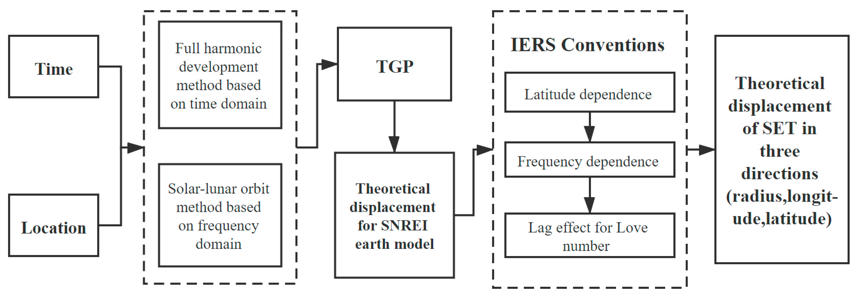
2.1.1. Tidal Displacement Model

The theoretical models of the SET, which are extensively used at present, take into account the influence of many complex factors, such as the earth’s ellipticity, rotation, inelasticity of the mantle, non-hydrostatic equilibrium, and lateral inhomogeneity. In this study, we refer to the principle of the DDW99 tidal model and the precise tidal correction parameters for the ground point displacement provided in the IERS Conventions [31,32]. The point displacement accuracy of the model can reach millimeter level [33]. The main process of the algorithm for the tidal displacement is demonstrated in Figure 1.

There exist two methods for calculating the TGP: the fully harmonic development method based on the frequency domain and the solar-lunar orbit method based on the time domain [34,35,36]. The fully harmonic development method exhibits high accuracy and is mainly used for precise SET observations, such as gravity tide observations. However, the displacement accuracy of this method exceeds that of the millimeter-level displacement model, resulting in substantial computational redundancy in calculating the high-density displacement distribution. The solar-lunar orbit method is based on the rules of celestial body movements and the laws of gravitation. The main factor affecting the accuracy of this method is the solution of the celestial calendar, which is less dependent on the correction of the ground station data. It is more suitable for macro-scale observation studies and analyses. Therefore, the time domain method was used to calculate the TGP in this work. The SET displacement in the SNREI earth can be obtained by:

$$\widehat{\delta r}={\displaystyle \sum }_{n=2}^3{h}_n\frac{W_n}{g_0}\widehat{e_r}+l_n\frac{\partial W_n}{g_0\partial \phi }\widehat{e_{\phi }}+l_n\frac{\partial W_n}{g_{0}cos\phi \partial \lambda }\widehat{e_{\lambda }},$$

(1)

where $n$ is the Legendre order, $W$ is the TGP, $h$ and $l$ are the Love number of the earth’s surface, $g_0$ is the mean surface gravity and $\widehat{e_r}$, $\widehat{e_{\phi }}$, and $\widehat{e_{\lambda }}$ are the three displacement components in the radius, latitude, and longitude directions, respectively.

Among them, the Love number consists of three parameters ($h$, $k$, and $l$) introduced in the early 20th century by Love and Shida T. It is used to characterize the elastic deformation of the earth’s interior materials. One of the main purposes of the SET research is to solve the Love number and study the elastic deformation characteristics of the earth’s interior. In this study, we used the theoretical values of the Love number from the IERS Conventions. The solid tidal displacement model was obtained by combining the displacement calculated in the SNREI earth with precise tidal correction. Considering the following factors, according to the requirements of the IERS Conventions, the accuracy of the tidal displacement model can reach the millimeter level:

• The latitude dependence and slight inter-band variations of Love number caused by the earth oblateness and the Coriolis force.
• The strong frequency dependence in the diurnal band and some other frequency dependence, owing to diurnal free oscillation resonance and inelastic mantle.
• The centrifugal force perturbation influenced by the inelastic mantle causing the Love number to lag behind the imaginary part of the TGP.

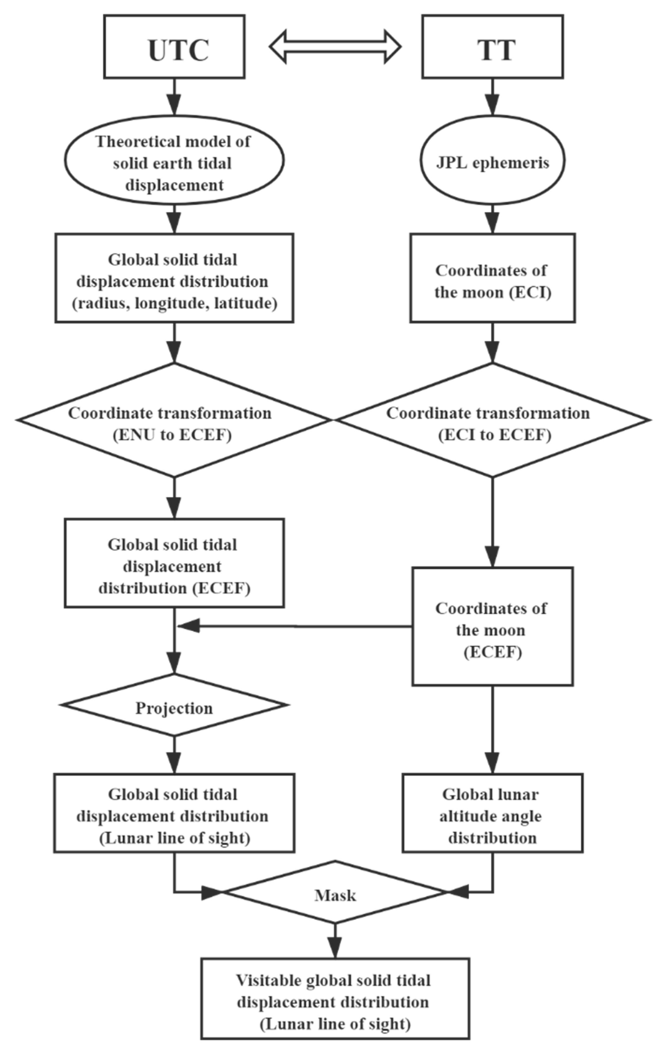
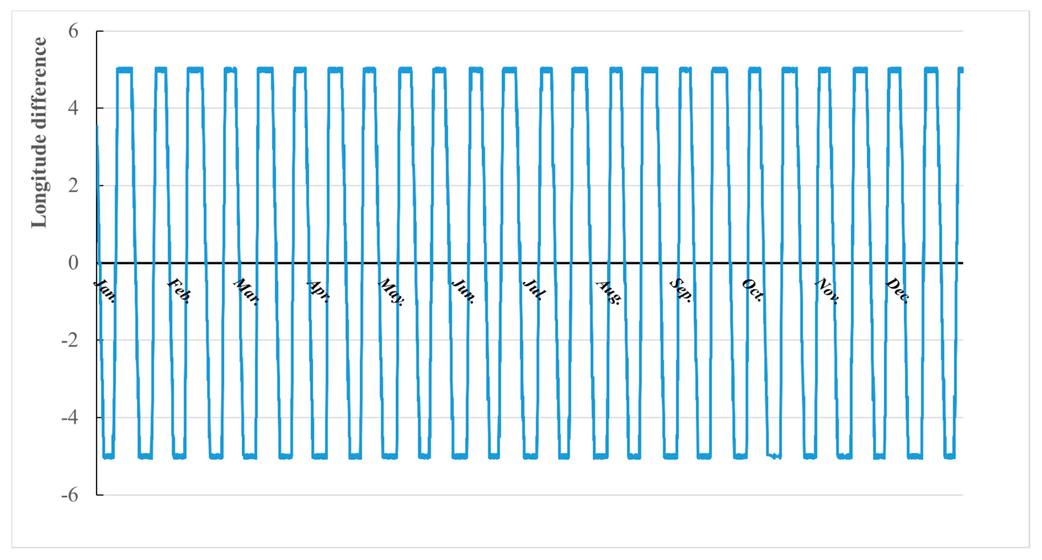
2.1.2. Lunar View Displacement Distribution

In order to determine the tidal displacement distribution from the lunar sensor’s view and ensure the visibility of the observation range, the key step is to obtain the lunar position information. The ephemeris can obtain the 3D rectangular coordinates (J2000 Earth Centered Inertial, ECI) of the sun, moon, and nine planets in the solar system via Fortran or C code provided by the JPL, which are available online at http://ssd.jpl.nasa.gov/. In this study, we used the DE430 ephemeris (created in 2013 covering the period from 1 January 1550 to 22 January 2650) of the JPL to obtain the trajectory of the moon. Then we combined it with the solid tidal model to obtain the spatial and temporal displacement characteristics from the lunar view [37]. The principal processes are presented in Figure 2.

When the displacement components are projected to the line-of-sight direction of the moon-based sensor, the influence of other factors on the observation geometry should also be considered, such as the specific position of the observation station on the moon, the axial precession, nutation, polar wandering, and free nutation of the earth. Therefore, we evaluated the magnitudes of these factors, as presented in

Table 1. Error of different influencing factors.

Factor	Error
Axial Precession	$\pm {10}^{-2}\mathrm{mm}$
Nutation	$\pm {10}^{-3}\mathrm{mm}$
Polar Wandering	$\pm {10}^{-4}\mathrm{mm}$
Free Nutation	$\pm {10}^{-4}\mathrm{mm}$
Position of Observation Station	$\pm 0.1\mathrm{mm}$

.

The error caused by the most significant factor in the table is 0.1 mm, which represents the projection difference of the observation platform location between the lunar center and the polar region. Previous studies have demonstrated that the establishment of a base in the low latitudes of the moon can better satisfy the observation geometry in remote sensing observation [38]. Therefore, neglecting the above factors in the calculation can also result in the simulation accuracy of millimeter levels. The position of the lunar center was used for the displacement projection in this simulation experiment.

The three directions of the tidal components are perpendicular to one another, and can be understood as a vector in the ENU coordinate system. Once the tidal displacement vector and lunar center position vector are unified into the ECEF coordinate system, the tidal displacement can be projected into the lunar direction according to the following formula:

$$x=|\overrightarrow{N}|cos\Theta ,$$

(2)

where $\overrightarrow{N}$ is the displacement vector, and $\Theta$ is the angle between the lunar center vector and displacement vector.

The lunar altitude angle at a certain point on the earth can be used as an indicator to judge whether or not the moon-based radar is visible. Additionally, the region with a positive altitude angle indicates that it is visible. The position vector of the lunar center $\widehat{r_{ENU}}$ can be obtained from the ECEF coordinate system, then the lunar altitude angle $\mathrm{Z}$ at any position on the earth’s surface can be calculated by Equation (3).

$$\mathrm{Z}=\arctan \left(\frac{\widehat{r_{ENU}}\left(3\right)}{\sqrt{\widehat{r_{ENU}}{\left(1\right)}^2+\widehat{r_{ENU}}{\left(2\right)}^2}}\right).$$

(3)

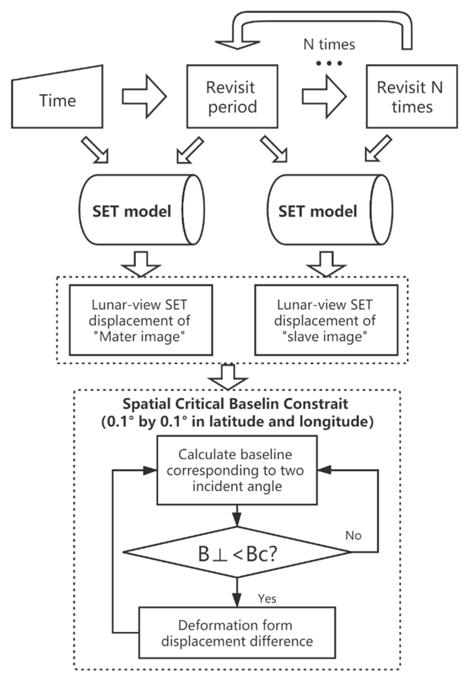
2.2. Simulation of Deformation Information

After comparing different interference measurement modes, we chose “single-station with repeat-pass” mode for the simulation experiment (the analyses are detailed in Section 3.2). InSAR is one kind of measurement technology which can extract the relative information of time and space. The measured deformation corresponds with the change of displacement between two time points. Therefore, the deformation measurement of SET we are discussing is obtained from the displacement difference between two time points. Additionally, the flowchart of its calculation is shown in Figure 3.

The revisit period was defined as the time difference in the same longitude of the subpoint (the annual average of the revisit period in 2018 was 24.84 h). With the change of the lunar declination in each revisit, the vertical baseline of moon-based InSAR will vary in the cross-track direction. The oversized vertical baseline is the main cause of geometrical decorrelation [39]. Additionally, the effective interference coverage needs to be screened through the critical baseline calculated by Equation (4) [40].

$$B_c=S_0\frac{B·\lambda }{c}tan\theta ,$$

(4)

where $\lambda$ is the wavelength, $B$ is the signal bandwidth, $c$ is the speed of light, $S_0$ is the distance between the radar and target, and $\theta$ is the average of incident angles. For lunar InSAR, the difference between the two incident angles is larger than that of the artificial satellite, which makes Equation (4) produce errors, and we compensated for them. The ratio of the vertical baseline to the critical baseline is related to the range resolution, and the range resolution can be defined by Equation (5) [41]. When the ratio $\mathsf{\alpha }$ reaches 0.99 with a 100 MHz of signal bandwidth, the corresponding range resolution is 150 m. It has a low impact on the observation of solid tide, so we took an infinite value of the ratio $\left(\mathsf{\alpha }=1\right)$ in this simulation work.

$${\rho }_{range}=\frac{c}{2\times B\left(1-\mathsf{\alpha }\right)}.$$

(5)

3. Simulation Results and Analyses

3.1. Tidal Displacement Characteristic

By comparing the three-direction displacement distribution at different time points, we found that the gradient of the solid tidal displacement distribution ranged from 0 mm/100 km to 10 mm/100 km in the vertical direction and 0mm/100 km to 2 mm/100 km in the horizontal direction. We selected a moment with a relatively larger gradient as a demonstration (Figure 4). The large gradient region tends to be concentrated near the maximum displacement (yellow region). It makes the SET in the swath of low-orbit SAR platforms always have no gradient. Additionally, this feature is very unfavorable for space observation.

Radar interferometry can capture the deformation information along the line-of-sight. When the range of radar incident angle is not considered, the SET displacement information from lunar view can be obtained by displacement projection and lunar altitude angle mask, as shown in Figure 5.

Taking the year 2018 as an example, we counted the displacement distribution from the lunar view in 8760 moments with a time interval of 1 h. From the displacement distribution and subpoint trajectory information, we determined the following spatial and temporal characteristics.

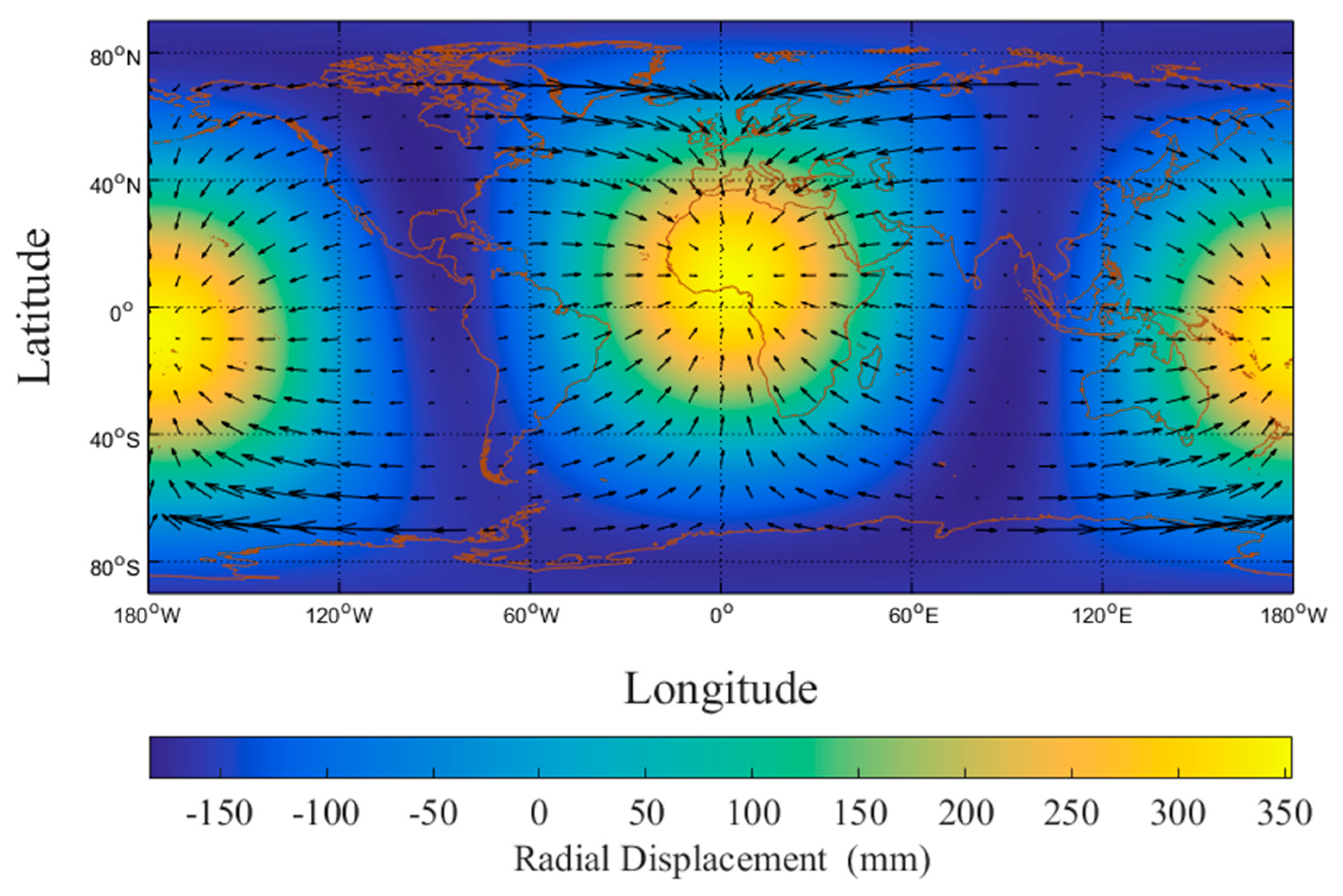
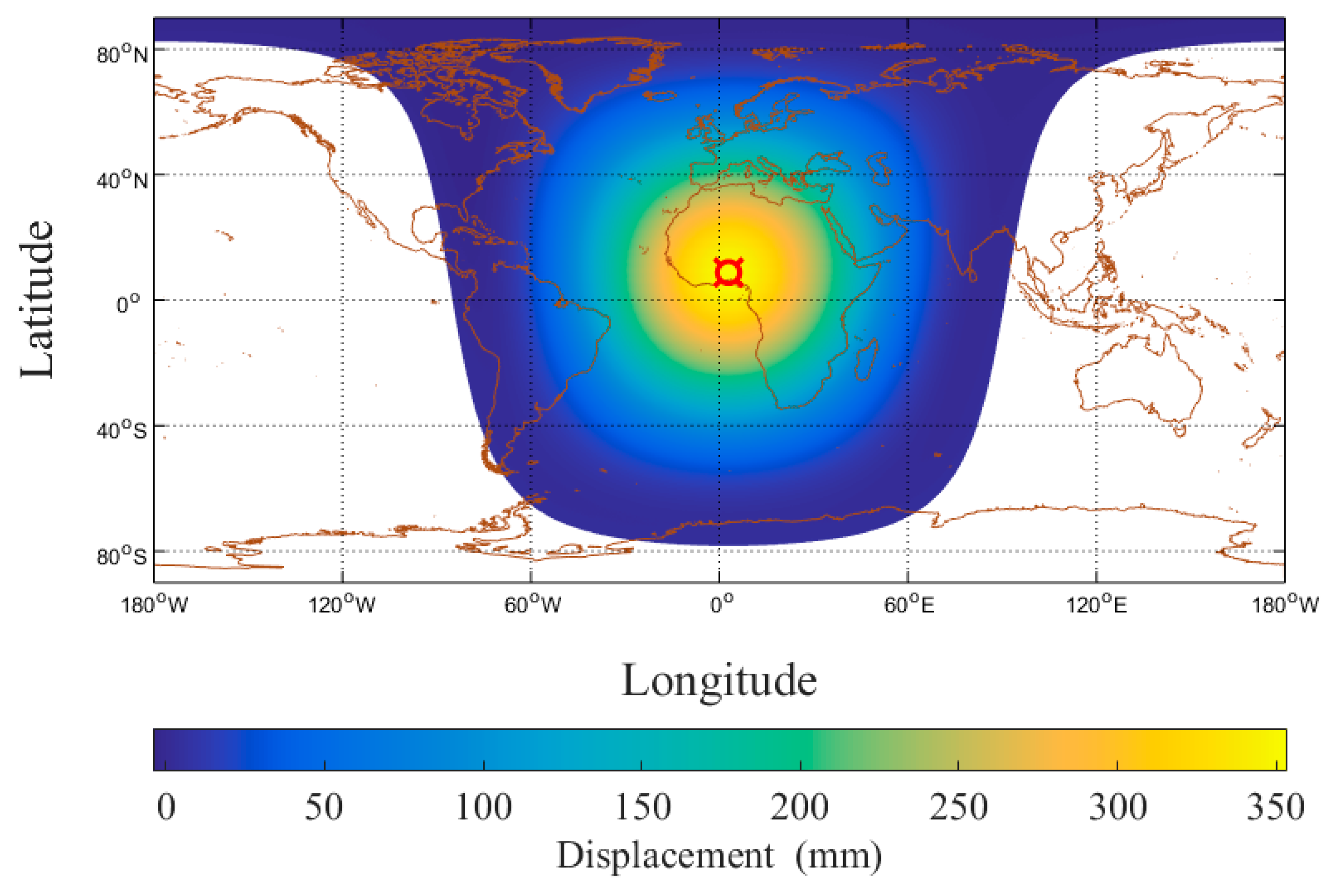
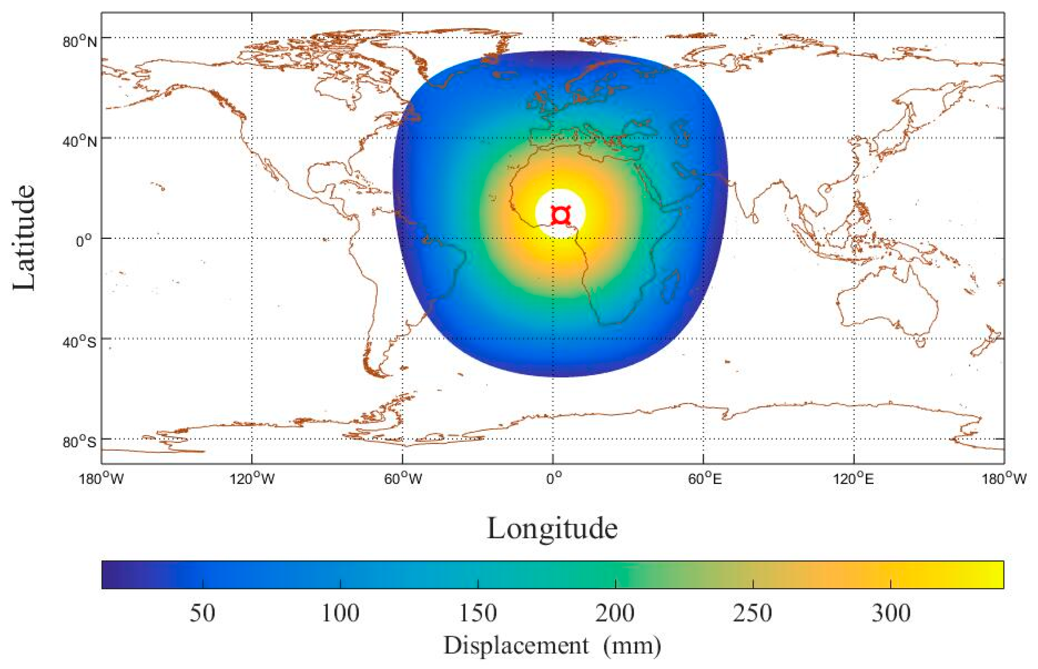
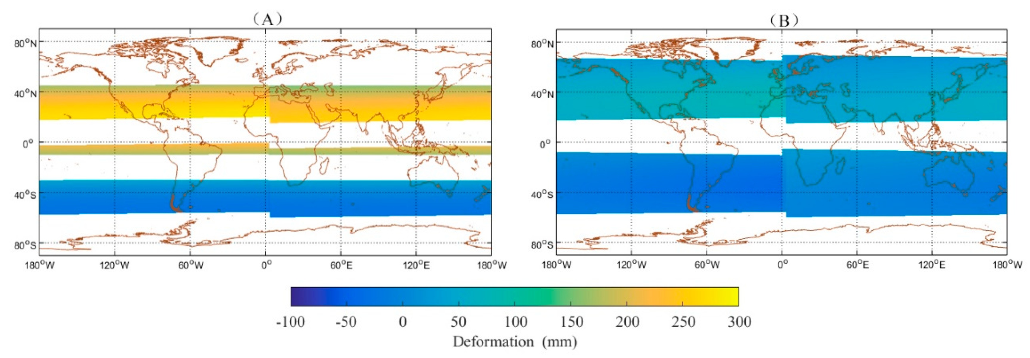
• The extreme point of the solid tidal displacement always appears near the lunar subpoint. Combined with the fact that there is always one side of the moon facing the earth, this feature makes the moon-based platform always have more abundant displacement information, which is not available on other artificial space satellite platforms. Although the difference calculation in interferometry can eliminate some of the displacement information, the change of the lunar subpoint in the cross-track direction ensures the existence of the deformation. As far as we know, the SET deformation information from lunar platform is most significant when compared with the low orbit platform and the geosynchronous orbit platform.
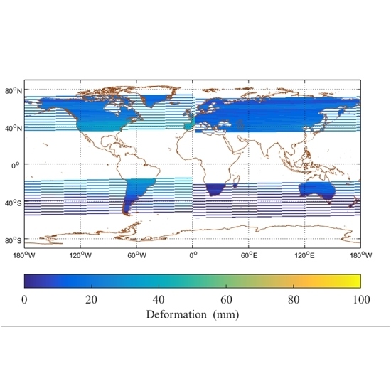
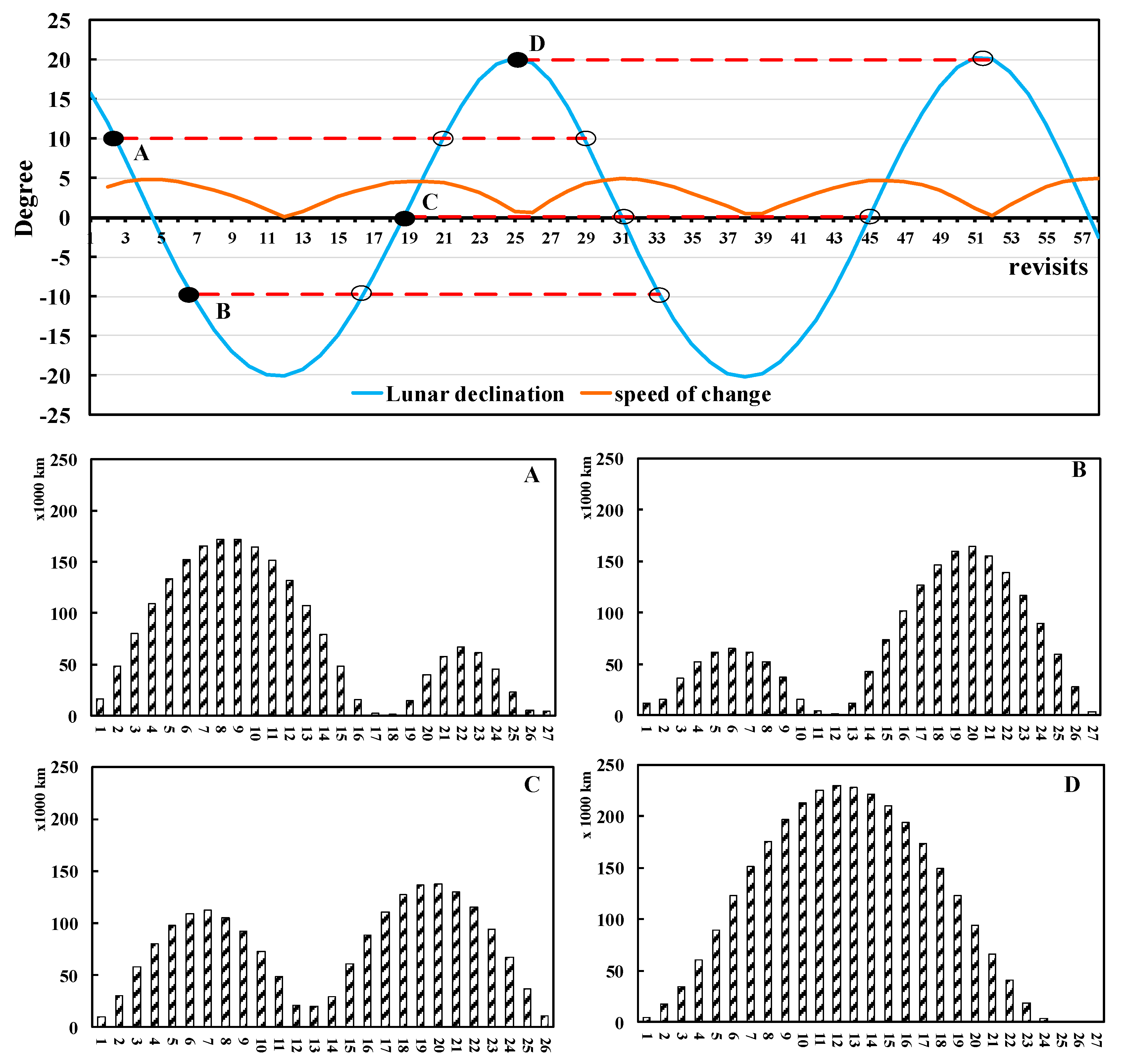
• It is difficult to observe the negative part of the SET displacement from the lunar view, and the displacement distribution decreases symmetrically from the extreme point to the surrounding area. We counted all time points with a maximum displacement of more than 300 mm, and found that 80% of them were concentrated in the time points corresponding to the middle and high lunar declination (7–21°).
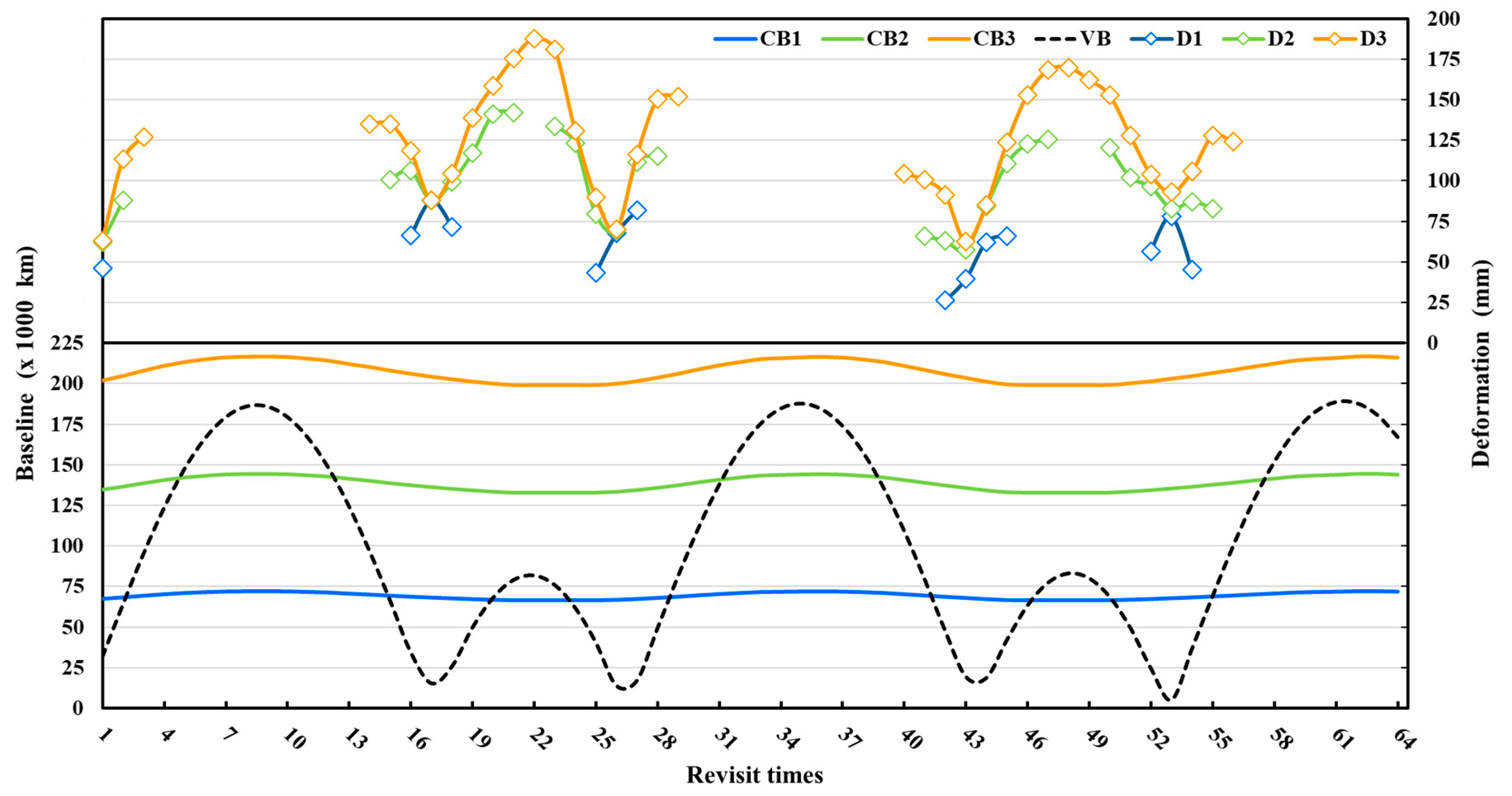
• The displacement distribution is constantly changing, and always exhibits some periodicity. Additionally, its periodic rule will gradually weaken with the increase of periodicity length. For example, the diurnal changes within the same month are more regular than those in different months. If the temporal baseline of interference is too short, it may reduce the deformation information due to the similar displacement states. On the contrary, if the temporal baseline is too long, other types of deformation may produce significant noise. There is a need to balance the two situations and to select the ideal temporal baseline. This characteristic makes the temporal resolution advantage of the lunar platform play an important role, its shortest temporal baseline of approximately one day allows us to make flexible choices.

3.2. Interferometry Mode and Observation Geometry

3.2.1. Interferometry Mode

Radar can be deployed in single or multiple station modes for interferometry on the moon. It is similar to the single-antenna repeat-pass mode and the dual-antenna mode of satellite SAR. We calculated the moon-based interference baseline at different revisit times. With the changes in the lunar declination, the spatial baseline length of the moon-based SAR will mainly vary in the range of 5000 to 200,000 km (as demonstrated in Figure 10), which is far beyond the baseline that can be generated between the stations on the moon (the moon diameter is about 3476 km). Due to the baseline ratio limitation, differential interferometry based on the multi-station mode has difficulty obtaining deformation information from different revisits. Moreover, the deployment of lunar stations brings a series of key problems, such as energy supply, data transmission, low temperature, lunar dust, and transportation costs. The costs incurred by these problems will multiply with the number of stations. Therefore, the single-station mode is more recommended in SET observation.

In the single-station mode, both the three-pass and four-pass D-InSAR require multiple temporal SAR data. This will make it inevitable to take into account the critical baseline and the baseline ratio in observation, which results in the SET information reduction in the deformation and texture features. In order to avoid these negative effects, it is better to combine the digital elevation model (DEM) in D-InSAR measurement. Therefore, the simulation experiments were carried out in the single-station with repeat-pass mode, as illustrated in Figure 6.

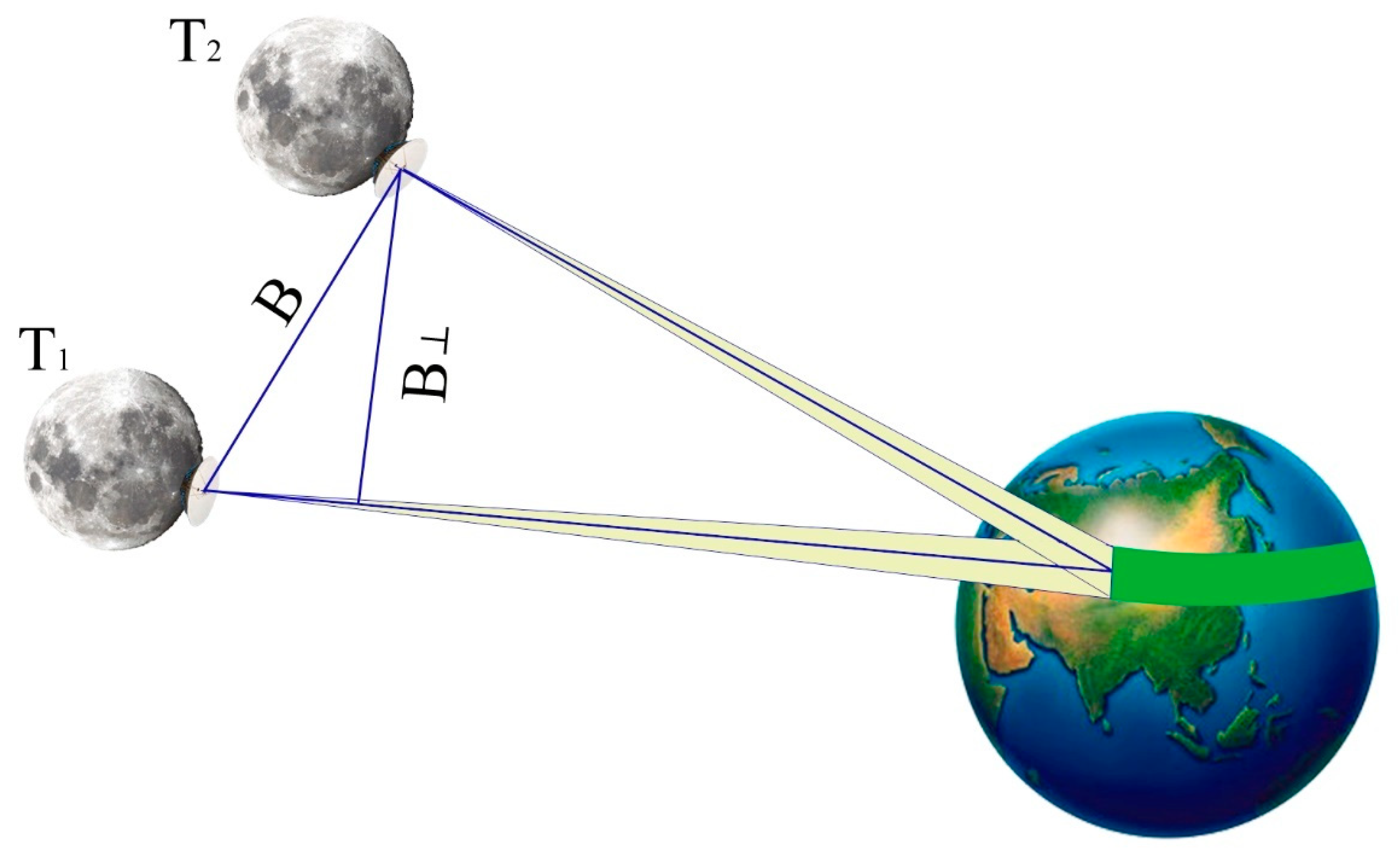
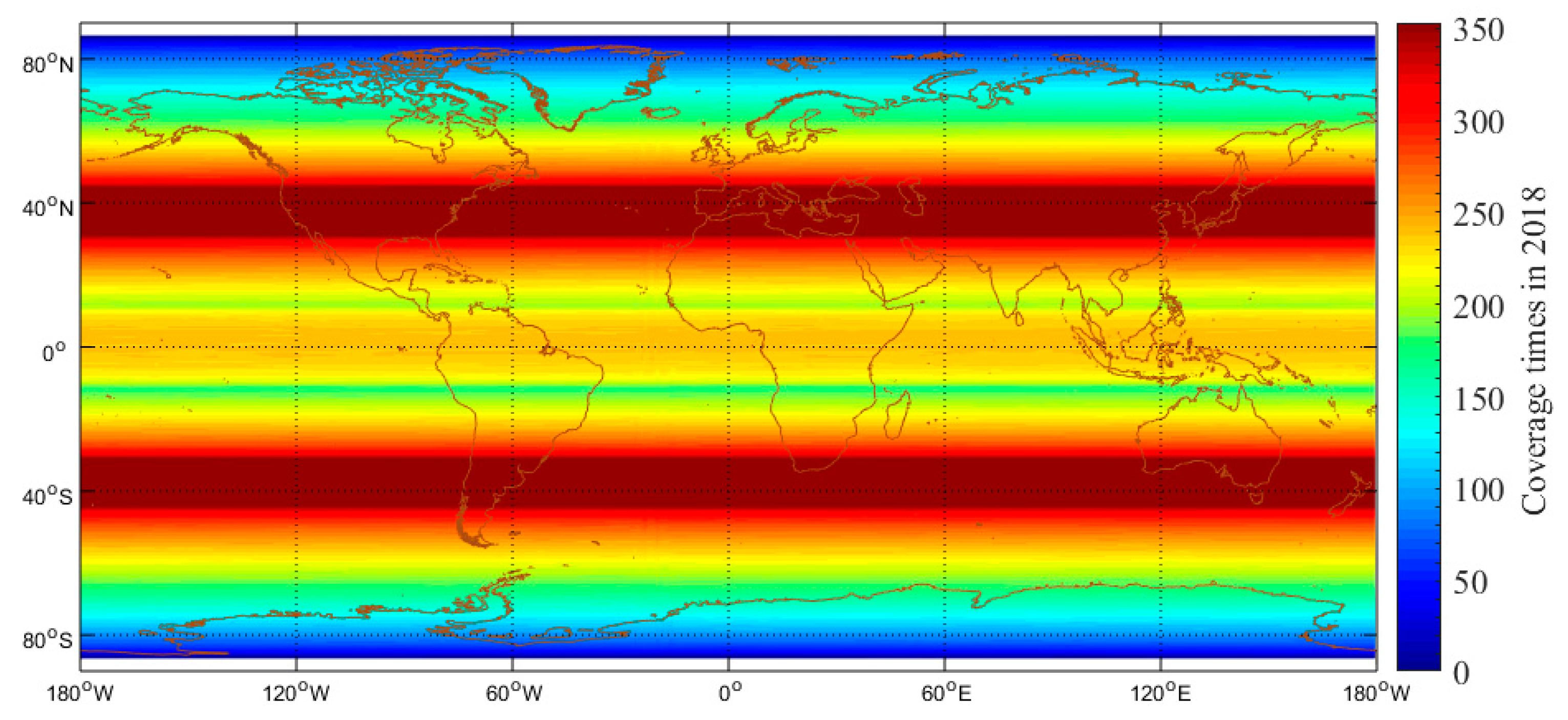
3.2.2. Observation Geometry

With the lunar revolution, the distance between the sensor and observation point varies slightly, and the earth rotation will be the main source of the Doppler shift. The azimuth direction of the lunar SAR imaging will be the same as the rotation direction of the earth, and the target will pass through the radar beam from west to east along the direction parallel to the equator. The incident angle of low earth orbit (LEO) satellites is usually 20° to 30°. In this range, the swath of lunar SAR is eight to nine times as wide as that of LEO satellites [42]. For the moon-based SAR, it only needs 2° of the FOV to observe half of the earth. If the side-looking imaging mechanism of the SAR is neglected, its instantaneous observation range is close to 50% of the earth’s surface. However, radar uses squint imaging to obtain line-of-sight deformations, resulting in the existence of inherent blind areas near the subpoint. Moreover, if the incident angle is excessively large, the backscattering energy will be attenuated, and the signal-to-noise ratio will be insufficient. Therefore, the actual observable range is constrained by the incident angle.

In this study, the range of the incident angle referred to typical parameters of the global change observation lunar based SAR (GCOLB-SAR) [43]. Additionally, some of its parameters are demonstrated in

Table 2. Typical parameters of global change observation lunar based SAR (GCOLB-SAR) (Partial).

Parameter (unit)	Value Range
Wavelength (cm)	24
Antenna Height (m)	57
Incident Angles (°)	10–66
Swath Width (km)	1680–2802
Signal Bandwidth (MHz)	100
Antenna Length (m)	198–837

.

We set the incident angle range of the lunar SAR to 10–66°, and the corresponding instantaneous optional scanning range with displacement information is illustrated in Figure 7.

The squint angle of the lunar SAR is defined as the angle between the antenna pointing and meridian plane passing through the lunar subpoint. By controlling this angle, the radar beam can cover the area with more tidal displacement, which makes D-InSAR obtain more deformation information. The longitude difference between the extreme point of the earth’s tidal displacement and lunar subpoint was calculated, as illustrated in Figure 8, which can provide a reference for the squint angle selection.

The chart indicates that the longitude difference is always less than 6°. Several conclusions about the squint angle when observing SET phenomena by the lunar SAR sensor can be drawn, as follows:

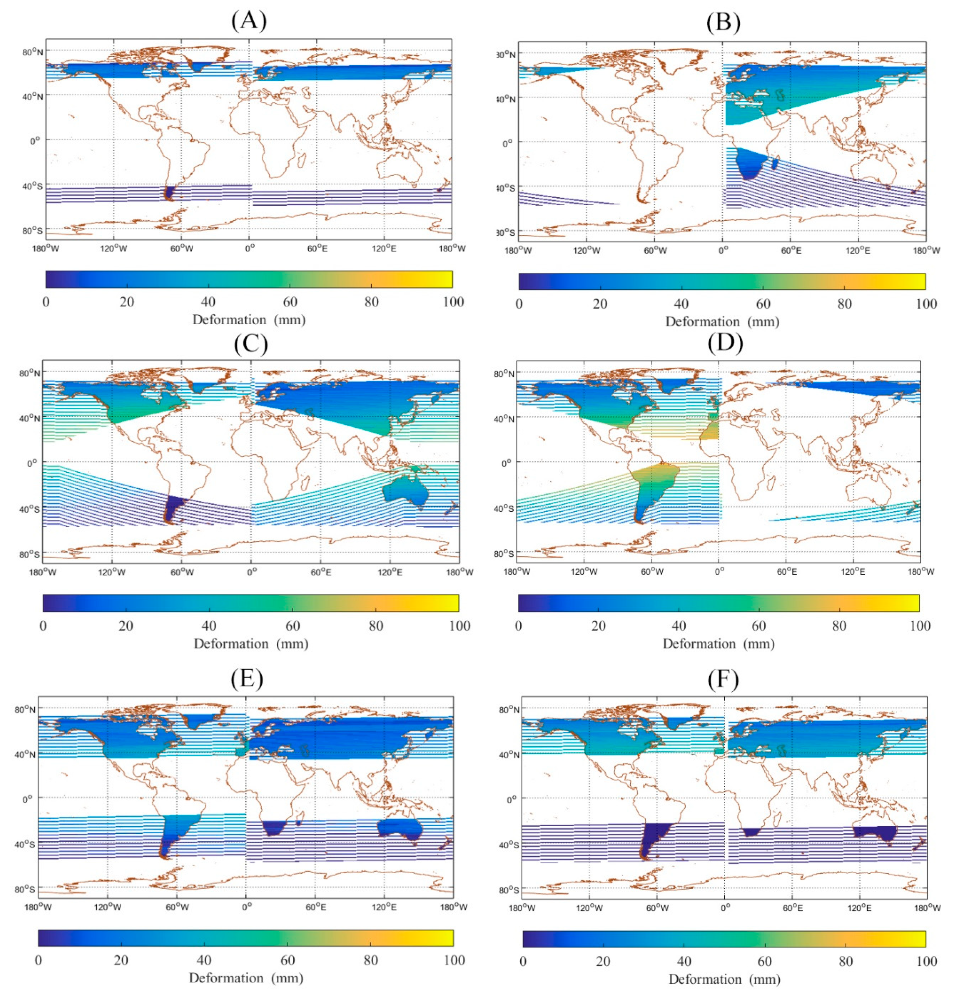
• In the whole period, the side-looking observation (the squint angle is 0) always has abundant SET information and is more recommended. If the lag effect of the tidal displacement on the TPG response is considered, backward-looking observation will be more appropriate (the antenna pointing to the east of the subpoint was defined as the backward-looking observation).
• When using side-looking observation, the observable range and tidal displacement are the largest. However, a blind area exists, which is approximately 9° north and south of the lunar subpoint. The squint angle is limited by the FOV, ranging from 0 to 1°. Different squint angle can reduce the blind area to some extent.

The side-looking observation will be used for further simulation work. The spatial coverage and SET information can be maximized while sacrificing the blind area close to the subpoint, and the imaging distortion caused by the earth’s curvature can be reduced. The temporal coverage with side-looking observation and incident angles of 10–66° is demonstrated in Figure 9. We can draw the following conclusions from it: (1) the temporal coverage at the same latitude is relatively uniform, and it changes significantly at the different latitude; (2) the observable region is approximately concentrated between 85° N and 85° S and the region with more than 200 revisits is approximately concentrated between 60° N and 60° S, which includes most of the terrestrial part of the earth.

3.3. Observation Effect under Three Signal Bandwidths

3.3.1. Selection of Master Image

The change of the lunar relative position between different revisits in the cross-track direction is the main source of spatial baseline. In addition, we can get the law of spatial baseline from the change of lunar declination. The complete period of the lunar declination is 18.6 years, and its small period is close to 27.3 days. We calculated the lunar declination in February and March 2018, and it will help us to determine a time point of the master image. In the process of interferometry, the different time points for master image will result in four cases of spatial baseline for slave images, as shown in Figure 10.

From the figure, we can see that the absolute value of the lunar declination had an opposite trend with its change speed. The revisits near the intersection of the red dotted line and lunar declination line more easily met the requirements of spatial baseline. When declination reaches a peak, its speed of change will decrease to the lowest. Additionally, the change speed of the lunar declination approximately varied from 0.1 to 5 degree/day. If the time point of the master image is selected with a low declination, the effective interference combinations (EICs) will be concentrated near three time points. However, the time point of the main image cannot have a too low declination, because this will cause the vertical baseline to have a fast change, and the number of EICs will decrease or even disappear.

When selecting the time point of the master image, we should first ensure that the lunar declination is not too low. Under the condition of meeting the spatial baseline requirement, we need to mainly consider the time points with rich SET displacement information, because too small vertical baseline is not good for solid tide observation, which will lead to the decrease of deformation information. In this study, we chose 2 March 2018 as the master image time point, which had a moderate lunar declination (12°), as marked as the red “¤” in Figure 10.

3.3.2. Deformation Information in EICs

We calculated the vertical baselines and critical baselines corresponding to 64 revisits from 0:00 on 2 March 20108. Additionally, the deformation distribution without a critical baseline constraint under different revisits was simulated, as illustrated in Figure 11. Compared to space-borne SAR, the time baseline of moon-based SAR is much shorter, with the minimum value being approximately 24.73 h, while the space baseline is much longer than that of the space-borne SAR. The vertical baseline length corresponding to Figure 11A,B reached 180,000 and 3000 km, respectively. The middle part of Figure 11A can be understood as the overlap area of the left-looking and right-looking observations at two moments. Of course, such a long baseline cannot be used for InSAR in any region of earth. The figure indicates that there was almost no gradient of the deformation distribution in the azimuth direction. It means that the requirements of the azimuth resolution and Doppler bandwidth for the moon-based SAR system are lower when observing the SET.

After the observable deformation was constrained by the critical baseline, the number of the EICs in the first period is 6, which are the 1st, 16th, 17th, 18th, 25th, and 26th revisits respectively (as shown in Figure 12.). When the effective interference area was less than 5% of the earth’s surface, those EICs would be abandoned. This is because the effective interferometric region is always strip-like and concentrated in high latitudes (large incident angle). If the deformation gradient in the swath decreases significantly, the advantage of the lunar SAR will become less meaningful. The calculation of the SET deformation distribution in EICs can provide a reference for the selection of the swath location.

In the above EICs calculation, the signal bandwidth corresponding to the critical baseline is 100 MHz. If a larger spatial baseline is available, it will be very beneficial for SET observation. This is because more EICs can be selected, and the larger spatial baseline in the cross-track direction will bring more deformation information. Furthermore, the SET information in each EIC will also increase. The most effective way for larger spatial baseline is to increase the wavelength or signal bandwidth, according to Equation (4). For the InSAR technology, L-band is a limit in interferometry, but the stable environment of the month-based platform can install more payload, which can provide the possibility for hundreds of MHz level of signal bandwidth. We hope to get the device requirement corresponding to the ideal SET observation effect. In this study, the observation effects with the signal bandwidths of 200 and 300 MHz were simulated and discussed, as illustrated in Figure 13. We used the deformation span to describe the amount of deformation information, and it was the difference between the maximum deformation value and the minimum deformation value in the effective observation region.

The change of the vertical baseline also has its own periodicity, and the length of the change period is approximately 26 or 27 revisits, as indicated by VB. The chart contains two change periods. In each change period, the deformation information of approximately 17th and 26th revisit periods hardly changes with the increase of the signal bandwidth. This is because the vertical baseline between these two revisits is relatively small and the effective observation region can reach the maximum in each EIC. In this case, the corresponding deformation span is approximately 8.8 and 7.0 cm, and after considering the swath width it will be reduced to 4 cm.

With the increase of the signal bandwidth, the EICs with larger spatial baselines can be selected, and additional tidal deformation information can be obtained. When the signal bandwidth increased to 200 MHz, four peak points of the deformation span appeared in each change period, which were located at the 2nd, 17th, 20th, and 23rd revisits in the first change period. When the signal bandwidth increased to 300 MHz, the deformation span exhibited a similar trend to the vertical baseline, and there were three extreme points which located at the 3rd, 14th, and 22nd revisits. It is because the latter two peak points were merged into one and appeared at the 22nd revisit. Among these, the deformation span of the 22nd revisit period is at the peak value, which is the ideal selection of the temporal baseline. In this case, after 300 MHz, the effects of increasing signal bandwidth level on deformation information will be no longer significant, because the deformation information is close to a limit.

We simulated different time points of the master image with high displacement information at these three bandwidths, and found that when the absolute value of declination corresponding to the master image time point was selected greater than 15°, the signal bandwidth level of 200 MHz can reach ideal observation effects, and about 50% time points for the master image were available. Additionally, when the absolute value of declination added 10–15°, the signal bandwidth level of 300 MHz can reach ideal observation effects, more than 75% time points for master image were available. The increase of signal bandwidth can rapidly increase the number of EICs, and then increase the observable SET information.

4. Discussion

With the rapid development of lunar exploration projects, there is increasing concern about the moon-based sensors. Many researchers believe that the moon is a good earth observation platform for geoscience phenomena. Based on the principle of remote sensing, many studies on the moon-based optical sensor and moon-based radar have been developed. However, few studies have addressed the observation requirements that the moon-based sensors need to meet for a specific geoscience phenomenon.

When the InSAR technology is applied to SET observation, there is a high space-time demand for the platform. Based on the temporal and spatial characteristics of the global tidal displacement, we found that it is important for the platform to have the advantage in the width of the swath, the flexibility of the EICs selection, and the gradient of relative displacement. These features make it possible to retain the unique texture of the displacement distribution, which is really important for SET observation. Compared with the low-orbit SAR platform and the inclined geosynchronous orbit SAR platform, the moon-based platform can better satisfy the observation requirements. The change of the lunar declination under different revisits is the main source of the deformation information for moon-based InSAR. We can see that the SET deformation span in the swath can reach several centimeters, which makes it possible to recognize it via texture information. This is difficult to reach for other observation platforms (in theory, the existing InSAR platform only has millimeter-level deformation span, and, for most of the time, it is lower than the millimeter level).

Based on the geometric constraints of the critical baseline, we found that the signal bandwidth of the system is very important for the observation of SET. As the range of optional spatial baseline becomes larger, the available master image time points and the number of EICs increase. In each EIC, the larger spatial baseline brings more deformation information, and the effective interference area in each EIC also increases.

Table 3. Observational effects of three signal bandwidths.

	100 MHz	200 MHz	300 MHz
Wavelength	24 cm	24 cm	24 cm
Number of EICs	13	26	33
Spatial coverage	27.80%	44.50%	51.60%
Deformation span	8.8 cm	14.2 cm	19.1 cm
Distance beam broadening	0.24°	0.24°	0.24°
Deformation span in swath	4.0 cm	7.1 cm	9.4 cm

displays the quantitative simulation results of the three signal bandwidths. We only counted the EICs in the first two periods. It can avoid other deformation except for the SET to some extent, and to reduce the time decorrelation. The spatial coverage is the average value of the ratio of the terrestrial area in EICs to the global terrestrial area, and it usually starts from the region with a large incident angle. In order to observe the tidal deformation in the area with small incident angle for a long time, the space coverage must be large enough.

The swath width can be determined by the beam width in the range direction, which is a function of the wavelength and antenna height. The beam width in the range direction, calculated from the parameters in Table 2, is 0.24°. The maximum deformation span obtained by adjusting the position of the swath is shown in Table 3. Obviously, this beam width is not very suitable for the SET observation. Provided that the swath width increases to about 3000–5300 km, almost all deformation information in the effective interference region will be retained, and the corresponding beam width in the range direction is 0.41°. A large swath width results in a longer time delay in the range direction of the beam and a rapid increase in the minimum antenna length and minimum antenna area. The optional range of pulse repetition frequency (PRF) and Doppler bandwidth can be reduced, then the maximum resolution of azimuth direction will be limited. However, for the observation of SET, the deformation gradient is mainly reflected in the cross-track direction.

When the signal bandwidth increases to 300 MHz level, the minimum optional absolute value of declination corresponding to the master image is 10°, which can cover approximately 75% time points with rich SET displacement. The number of EICs as well as the spatial coverage will also increase, and more than 50% of the terrestrial region can be monitored. After 300 MHz, the deformation span will be close to the limit, and the effects of increasing signal bandwidth will be no longer significant. The moon-based InSAR can achieve ideal SET observation effects using these system parameters. Of course, the observation potential of moon-based platforms to SET in the north and south poles of the earth may not be as good as that of artificial satellites. This is not only because the change of SET at the poles is weak, but also because of the limitation of the maximum incident angle. Furthermore, the large swath and signal bandwidth have high requirements on the antenna design and frequency modulation mode, which is a challenge to engineering development. Therefore, it is necessary to synthesize the observation requirements and engineering development to determine the ideal system parameters of the lunar InSAR.

5. Conclusions

With the aim of meeting the space observation requirements of the SET, this study discussed the possibility of observation by InSAR technology from a moon-based remote sensing platform, which may provide a reference for the design of sensors in the future. The following contributions have been made in the simulation work:

(1) The moon-based sensor can always observe the regions with more abundant information of the SET. It was found that the extreme point of the displacement always appeared near the lunar subpoint. The lunar InSAR can obtain rich SET deformation by cross-track direction difference.

(2) The single-station with repeat-orbit mode as well as the side-looking SAR imaging are more suitable for the D-InSAR measurement of the SET on the moon. It can reduce the engineering costs while avoiding the baseline ratio constraints and the unique texture information destruction. The side-looking mode can maximize the spatial coverage and deformation information while reducing the imaging distortion caused by the curvature of the earth.

(3) A large signal bandwidth as well as swath width are required to make full use of the advantages of the lunar platform in observing the SET. The signal bandwidth of 300 MHz level is recommended. After 300 MHz, the deformation information will be close to the limit, and the effects of increasing signal bandwidth on SET will be no longer significant. The swath width of 3000–5300 km is more recommended, and the corresponding beam width in the range direction is 0.41°. On this condition, almost all deformation information in the effective interference region is retained. Although the maximum resolution of azimuth direction is limited, it is not serious for SET observation.

In summary, referring to the global characteristics of the SET phenomenon and advantages of the moon-based platform, the moon can become a new platform for the solid earth observation. The results of this study demonstrate that the large swath of the moon-based InSAR and its effective space-time continuity can better satisfy the macroscopic observation of solid earth phenomena. In future work, more in-depth simulation analysis will be done, and it is necessary to consider the impacts of various factors on moon-based observation, such as the ionosphere contribution for L band, synthetic aperture time, and the power budget for the SAR system. We anticipate additional research results on lunar imaging radar, which will contribute to the observation of macroscopic earth phenomena.

References

1. Guo, J.Y. The Fundamentals of Geophysics; Surveying and Mapping Press: Beijing, China, 2001. [Google Scholar]
2. Melchior, P. The Tides of Planet Earth, 2nd ed.; Pergamon: Oxford, UK, 1983. [Google Scholar]
3. Goodkind, J.M. The superconducting gravimeter. Rev. Sci. Instrum. 1999, 70, 4131–4152. [Google Scholar] [CrossRef] [Green Version]
4. Fang, J. The Solid Earth’s Tides; Science Press: Beijing, China, 1984. [Google Scholar]
5. Zhang, G.; Xu, J.; Wang, X. International trends and progress of solid tide observation and research. J. Seismol. Res. 2004, 27, 104–107. [Google Scholar]
6. Nige, T.P.; Matt, A.K.; Mike, P.S. GPS height time series: Short-period origins of spurious long-period signals. J. Geophys. Res. Solid Earth 2007, 112, B02402. [Google Scholar]
7. Watson, C.; Tregoning, P.; Coleman, R. Impact of solid Earth tide models on GPS coordinate and tropospheric time series. Geophys. Res. Lett. 2006, 33, 1–4. [Google Scholar] [CrossRef] [Green Version]
8. Ferretti, A.; Montiguarnieri, A.; Prati, C.; Rocca, F.; Massonet, D. InSAR principles-guidelines for SAR interferometry processing and interpretation. J. Financ. Stab. 2007, 10, 156–162. [Google Scholar]
9. Wright, T.J.; Parsons, B.; England, P.C.; Fielding, E.J. InSAR Observations of Low Slip Rates on the Major Faults of Western Tibet. Science 2004, 305, 236–239. [Google Scholar] [CrossRef] [Green Version]
10. Delacourt, C.; Briole, P.; Achache, J.A. Tropospheric corrections of SAR interferograms with strong topography. Application to Etna. Geophys. Res. Lett. 1998, 25, 2849–2852. [Google Scholar] [CrossRef]
11. Lu, Z.; Wicks, C.; Power, J.A.; Dzurisin, D. Ground deformation associated with the March 1996 earthquake swarm at Akutan volcano, Alaska, revealed by satellite radar interferometry. J. Geophys. Res. 2000, 105, 21483–21495. [Google Scholar] [CrossRef] [Green Version]
12. Zhao, C.Y.; Zhang, Q.; Ding, X.L.; Lu, Z.; Yang, C.S.; Qi, X.M. Monitoring of land subsidence and ground fissures in Xian, China 2005-2006: Mapped by SAR interferometry. Environ. Geol. 2009, 58, 1533–1540. [Google Scholar] [CrossRef]
13. Stevens, N.F.; Wadge, G.; Williams, C.A.; Morley, J.G.; Muller, J.P.; Murray, J.B. Surface movements of emplaced lava flows measured by synthetic aperture radar interferometry. J. Geophys. Res. 2001, 106, 11293–11313. [Google Scholar] [CrossRef]
14. Hao, J.; Wu, T.; Wu, X.; Hu, G.; Zou, D.; Zhu, X.; Lin, Z.; Li, R.; Xie, C.; Ni, J.; et al. Investigation of a Small Landslide in the Qinghai-Tibet Plateau by InSAR and Absolute Deformation Model. Remote. Sens. 2019, 11, 2126. [Google Scholar] [CrossRef] [Green Version]
15. Ramsey, E.; Lu, Z.; Rangoonwala, A.; Rykhus, R. Multiple Baseline Radar Interferometry Applied to Coastal Land Cover Classification and Change Analyses. GIScience Remote. Sens. 2006, 43, 283–309. [Google Scholar] [CrossRef] [Green Version]
16. Zebker, H.A.; Werner, C.L.; Rosen, P.; Hensley, S. Accuracy of Topographic Maps Derived from ERS-1 Interferometric Radar. IEEE Trans. Geosci. Remote. Sens. 1993, 32, 823–836. [Google Scholar] [CrossRef] [Green Version]
17. Williams, C.A.; Wadge, G. An accurate and efficient method for including the effects of topography in three dimensional elastic models of ground deformation with applications to radar interferometry. J. Geophys. Res. 2000, 105, 8103–8120. [Google Scholar] [CrossRef]
18. Carnec, C.; Fabriol, H. Monitoring and modeling land subsidence at the Cerro Prieto geothermal field, Baja California, Mexico, using SAR interferometry. Geophys. Res. Lett. 1999, 26, 1211–1214. [Google Scholar] [CrossRef]
19. Huang, Z.; Zhang, G.; Shan, X.; Gong, W.; Zhang, Y.; Li, Y. Co-Seismic Deformation and Fault Slip Model of the 2017 Mw 7.3 Darbandikhan, Iran–Iraq Earthquake Inferred from D-InSAR Measurements. Remote. Sens. 2019, 11, 2521. [Google Scholar] [CrossRef] [Green Version]
20. Hooper, A.; Bekaert, D.; Spaans, K.; Arikan, M. Recent advances in SAR interferometry time series analysis for measuring crustal deformation. Tectonophysics 2011, 514, 1–13. [Google Scholar] [CrossRef]
21. Qiao, S.; Sun, F.; Zhu, X.; Li, J.; Cong, M. Application of GPS/VLBI/SLR/InSAR Combination in Geodynamics. J. Geod. Geodyn. 2004, 24, 92–97. [Google Scholar]
22. Farolfi, G.; Ventisette, C.D. Monitoring the Earth’s ground surface movements using satellite observations-Geodynamics of the Italian peninsula determined by using GNSS networks. In Proceedings of the IEEE International Workshop on Metrology for Aerospace, Florence, Italy, 22–23 June 2016. [Google Scholar]
23. Colesanti, C.; Ferretti, A.; Prati, C. Monitoring landslides and tectonic motions with the Permanent Scatterers Technique. Eng. Geol. 2003, 68, 3–14. [Google Scholar] [CrossRef]
24. Bruno, D.; Hobbs, S.; Ottavianelli, G. Geosynchronous synthetic aperture radar: Concept design, properties and possible applications. Acta Astronaut. 2006, 59, 149–156. [Google Scholar] [CrossRef]
25. Bruno, D.; Hobbs, S.E. Radar Imaging from Geosynchronous Orbit: Temporal Decorrelation Aspects. IEEE Trans. Geosci. Remote Sens. 2010, 48, 2924–2929. [Google Scholar] [CrossRef]
26. Crawford, I.A. Back to the Moon: The scientific rationale for resuming lunar surface exploration. Planet. Space Sci. 2012, 74, 3–14. [Google Scholar] [CrossRef] [Green Version]
27. Racca, G.D.; Foing, B.H.; Coradini, M. Smart-1: The First Time of Europe to the Moon; Wandering in the Earth–Moon Space. Earth-Moon Relationships. 2001, pp. 379–390. Available online: https://link.springer.com/chapter/10.1007/978-94-010-0800-6_32 (accessed on 1 November 2019).
28. Zheng, Y.; Ouyang, Z.; Li, C.; Liu, J.; Zou, Y. China’s lunar exploration program: Present and future. Planet. Space Sci. 2003, 56, 881–886. [Google Scholar] [CrossRef]
29. Fornaro, G.; Franceschetti, G.; Lombardini, F.; Mori, A.; Calamia, M. Potentials and limitations of Moon-Borne SAR imaging. IEEE Trans. Geosci. Remote Sens. 2010, 48, 3009–3019. [Google Scholar] [CrossRef]
30. Guo, H.D.; Liu, G.; Ding, Y.X. Moon-based Earth observation: Scientific concept and potential applications. Int. J. Digit. Earth. 2017, 11, 546–557. [Google Scholar] [CrossRef]
31. Dehant, V.; Defraigne, P.; Wahr, J.M. Tides for a convective Earth. J. Geophys. Res. 1999, 104, 1035–1058. [Google Scholar] [CrossRef]
32. IERS. IERS Technical Note. 2003 N0.32. Available online: https://www.iers.org/IERS/EN/Publications/TechnicalNotes/TechnicalNotes.html (accessed on 27 December 2019).
33. Xu, H. Solid Earth Tides; Hubei Science & Technology Press: Wuhan, China, 2010. [Google Scholar]
34. Hartmann, T.; Wenzel, H.G. The HW95 tidal potential catalogue. Geophys. Res. Lett. 1995, 22, 3553–3556. [Google Scholar] [CrossRef]
35. Xi, Q.W. The precision of the development of the tidal generating potential and some explanatory notes. Chin. J. Geophys. 1989, 2, 182–194. [Google Scholar]
36. Hartmann, T.; Wenzel, H.G. The harmonic development of the Earth tide generating potential due to the direct effect of the planets. Geophys. Res. Lett. 1994, 21, 1991–1993. [Google Scholar] [CrossRef]
37. Folkner, W.M.; Williams, J.G.; Boggs, D.H.; Park, R.S.; Kuchynka, P. The Planetary and Lunar Ephemerides DE430 and DE431. Interplanet. Netw. Prog. Rep. 2014, 42, 1–81. [Google Scholar]
38. Ren, Y.; Guo, H.; Liu, G.; Ye, H. Simulation Study of Geometric Characteristics and Coverage for Moon-Based Earth Observation in the Electro-Optical Region. IEEE J. Sel. Top. Appl. Earth Obs. Remote. Sens. 2017, 10, 2431–2440. [Google Scholar] [CrossRef]
39. Xia, Y. Synthetic Aperture Radar Interferometry; Springer: Berlin, Heidelberg, 2010. [Google Scholar]
40. Zhang, F.; Ma, D.B.; Pei, H.N. Analysis of the Elements of Baseline Estimation of Interferometric SAR. Remote. Sens. Inf. 2005, 3, 7–9. [Google Scholar]
41. Meyer, F.J.; Sandwell, D.T. SAR interferometry at Venus for topography and change detection. Planet. Space Sci. 2012, 73, 130–144. [Google Scholar] [CrossRef] [Green Version]
42. Ding, Y. Moonborne Earth Observation Synthetic Aperture Radar and Its Application in Global Change. Ph.D. Thesis, Graduate School of Chinese Academy of Sciences, Beijing, China, 10 July 2014. [Google Scholar]
43. Guo, H.D.; Ding, Y.X.; Liu, G.; Zhang, D.W.; Fu, W.X.; Zhang, L. Conceptual study of lunar-based SAR for global change monitoring. Sci. China Earth Sci. 2014, 57, 1771–1779. [Google Scholar] [CrossRef]
Figure 1. Flowchart of theoretical tidal displacement model. After inputting the time and location information, the tide-generating potential (TGP) can be calculated by using the time domain or frequency domain algorithm, and it is then converted into displacement information in a spherically stratified and non-rotating earth with perfectly elastic and isotropic structural relation (SNREI Earth). The theoretical values of the tidal displacement with millimeter accuracy can be obtained by precise tidal correction based on the IERS Conventions.
Remotesensing 12 00123 g001
Figure 2. Flowchart of displacement distribution from lunar view. The time input into the tidal model and Jet Propulsion Laboratory (JPL) ephemeris are coordinated universal time (UTC) and terrestrial time (TT), respectively. The three components of the solid earth tides (SET) displacement point to the same direction as the local Cartesian coordinates coordinate system (ENU). Then, the displacement information and position information of the moon are unified into the earth-centered, earth-fixed coordinate system (ECEF). After the displacement projection, the displacement distribution of the SET is masked by the observable range obtained from the lunar altitude angle.
Remotesensing 12 00123 g002
Figure 3. Flowchart of the calculation of the spatiotemporal baseline and SET deformation in the effective interference region. The scanning trajectory of lunar synthetic aperture radar (SAR) is approximately parallel to the equator, as shown in Figure 6. The relationship between the longitude of lunar subpoint and accurate time point is established according to the ephemeris data. After inputting a start time of the master image, the revisit period can be determined. Additionally, the accurate time points of various longitudes as well as the start time of next scan can be calculated (assuming that the earth rotates at a constant speed). In this way, the displacement matrices under multiple revisits can be obtained by inputting longitude, latitude, and time point into the SET model. The vertical baseline ( B ) matrix as well as the critical baseline ( B c ) matrix can be obtained via the ECEF coordinates of lunar center and the incident angle matrix (according to the lunar altitude angle matrix). The deformation matrices in effective interference regions under multiple revisits can be obtained through the displacement matrices difference and the critical baseline constraint ( B < B c ) at every latitude and longitude.
Remotesensing 12 00123 g003
Figure 4. Global displacement distribution at 0:00 on 2 March 2018. The black arrows represent the direction of the horizontal displacement. The vertical displacement is from the earth’s center and distinguished by different colors. In order to retain the information of various gradients, the latitudinal and longitudinal density of the displacement distribution should be no less than 0.5°. This figure was generated in MATLAB with a density of 0.1°.
Remotesensing 12 00123 g004
Figure 5. Global displacement distribution in moon direction at 0:00 on 2 March 2018. The image is obtained by masking the projected displacement distribution in the area with a negative lunar altitude angle. The non-displacement area is the absolute blind area of the lunar sensor at that time. The sum of the tidal displacements is distinguished by different colors, and the red “¤” sign indicates the lunar subpoint.
Remotesensing 12 00123 g005
Figure 6. Single-station observation geometry of moon-based interferometric synthetic aperture radar (InSAR). The T1 and T2 represent two different time points.
Remotesensing 12 00123 g006
Figure 7. Global displacement distribution in moon direction with incident angle constraint of 10–66° at 0:00 on 2 March 2018.
Remotesensing 12 00123 g007
Figure 8. Longitude difference between extreme point of earth’s tidal displacement and lunar subpoint in 8760 phases in 2018.
Remotesensing 12 00123 g008
Figure 9. Temporal coverage in 2018 (side-looking, 10–66° incident angle).
Remotesensing 12 00123 g009
Figure 10. Lunar declination in February and March 2018, as well as the four cases for the change of spatial baseline. The horizontal axis represents the revisit times. The vertical axis of the upper figure represents the lunar declination. The blue line and the orange line represent the trend of declination and its own change speed, respectively. (AD) represent the change trend of spatial baseline in different revisits when the time point of the master image was located at the lunar declination shown in the upper figure.
Remotesensing 12 00123 g010
Figure 11. (A) and (B) represent the deformation distribution of the 8th and 16th revisits from 0:00 on 2 March 2018, respectively. The upper and lower parts of (B) can be understood as the observable deformation region of the lunar SAR from the right-looking and left-looking, respectively.
Remotesensing 12 00123 g011
Figure 12. SET deformation distribution of all effective interference combinations (EICs) in the first change period of vertical baseline. (AF) represent the 1st, 16th, 17th, 18th, 25th, and 26th revisits, respectively. The stripe like area represents the effective interference area of lunar SAR, and the deformation value of the terrestrial part is distinguished by different colors.
Remotesensing 12 00123 g012
Figure 13. The three CB lines represent the maximum value of the critical baseline, and CB1, CB2, and CB3 have a signal bandwidth of 100, 200, and 300 MHz, respectively; VB represents the vertical baseline; and D1, D2, and D3 represent the tidal deformation span in an EIC.
Remotesensing 12 00123 g013