Article

Long-Term Satellite Image Time-Series for Land Use/Land Cover Change Detection Using Refined Open Source Data in a Rural Region

Centre for Geographical Studies, Institute of Geography and Spatial Planning, Universidade de Lisboa, Rua Branca Edmée Marques, 1600-276 Lisboa, Portugal
*
Author to whom correspondence should be addressed.
Remote Sens. 2019, 11(9), 1104; https://doi.org/10.3390/rs11091104
Submission received: 31 March 2019 / Revised: 3 May 2019 / Accepted: 6 May 2019 / Published: 9 May 2019
(This article belongs to the Special Issue Open Resources in Remote Sensing)

Abstract

:
The increasing availability and volume of remote sensing data, such as Landsat satellite images, have allowed the multidimensional analysis of land use/land cover (LULC) changes. However, the performance of image classification is highly dependent on the quality and quantity of the training set and its temporal continuity, which may affect the accuracy of the classification and bias the analysis of the LULC changes. In this study, we intended to apply a long-term LULC analysis in a rural region based on a Landsat time series of 21 years (1995 to 2015). Here, we investigated the use of open LULC source data to provide training samples and the application of the K-means clustering technique to refine the broad range of spectral signatures for each LULC class. Experiments were conducted on a predominantly rural region characterized by a mixed agro-silvo-pastoral environment. The open source data of the official Portuguese LULC map (Carta de Uso e Ocupação do Solo, COS) from 1995, 2007, 2010, and 2015 were integrated to generate the training samples for the entire period of analysis. The time series was computed from Landsat data based on the normalized difference vegetation index and normalized difference water index, using 221 Landsat images. The Time-Weighted Dynamic Time Warping (TWDTW) classifier was used, since it accounts for LULC-type seasonality and has already achieved promising overall accuracy values for classifications based on time series. The results revealed that the proposed method was efficient in classifying a long-term satellite time-series with an overall accuracy of 76%, providing insights into the main LULC changes that occurred over 21 years.

1. Introduction

The increased availability of free and analysis-ready remote sensing (RS) data, such as Landsat, supports dynamic analysis in time and space [1,2], since it allows researchers to perform multidimensional classifications of land use/land cover (LULC) based on satellite image time series [3,4,5]. In fact, the classification methods involving multitemporal remotely sensed images are becoming a trend in LULC change detection [6] and also in detailed LULC classification approaches [7], since these are reported to achieve better results than single-date classification methods [8,9,10]. Particularly due to the developed and improved tools and algorithms that give priority to time dimension in satellite data analysis [11,12], the changes and disturbances of LULC classes can now be more easily detected.
As Zhu and Woodcock [6] emphasized, the ability to accurately identify LULC changes using remote sensing data depends on an algorithm that can use high spatial resolution data and is based on a multitemporal analysis. However, the multitemporal analysis application can have some limitations—for example, vegetation phenology, sun angles, clouds, sensor errors, among others [6]. Likewise, concerning the well-established, advanced, nonparametric classifiers in remote sensing literature [8,13], such as the support vector machine (SVM) and the random forest (RF) [14], it has been recognized that some challenges still remain regarding LULC classifications based on time series [15]. These challenges are: (i) the inexistence/existence and the quality of the samples required to train the algorithm, (ii) the irregular phenological signatures of different LULC types through time, and (iii) the absence of a data temporal continuum [15].
The Dynamic Time Warping (DTW) classifier has been demonstrated to be a capable solution to deal with some of these challenges [15,16]. Since it can “fill-in” temporal gaps in the remote sensing time series (e.g., cloudy images), it has been successfully applied in satellite imagery time-series analysis [17,18]. However, the distinctive phenological cycle of each LULC class requires an equilibrium between shape matching and temporal alignment [19,20], which is why Maus et al. [21] improved the DTW algorithm. Maus et al. [21] proposed the Time-Weighted Dynamic Time Warping (TWDTW) method that includes time-weighting to account for seasonality. This yields better time series to benefit the LULC mapping. In the research of Maus et al. [18], this method was applied to the LULC classification of a tropical forest area from MODIS enhanced vegetation index (EVI) data. It had the highest accuracy for the forest, pastures, single cropping and double cropping classes’ classification and an overall accuracy of about 87%. Belgiu and Csillik [22] evaluated the TWDTW method for mapping different cropland types in two European cities (in Italy and Romania) and one American city (in California) from Sentinel-2 normalized difference vegetation index (NDVI) time series. In their research, this method achieved a higher overall accuracy when classifying different cropland classes in the two European study areas compared to the classification results of the RF method [22]. Also, the TWDTW method proved it could produce good output in terms of mapping accuracy, even with few training samples [15,23].
In addition, it is not only the absence of LULC reference data to train the algorithm that can be detrimental to the image classification results but also the lack of representative samples for each LULC class [24]. If we look into the literature regarding the acquisition of training samples, they are usually acquired from field surveys or expert knowledge through the visual interpretation of other products—for example, high-resolution images from Google Earth and aerial photographs [24]. However, collecting training samples from fieldwork involves high associated costs, in terms of money and time, and collecting training samples through visual interpretations can be difficult, due to the lack of available products, causing biases in the representation of the samples [25]. Various approaches have been used to overcome the lack insufficient training samples, such as semi-supervised learning or, more recently, active learning [26,27]. However, both these approaches are dependent on preexisting labelled samples, which require user expertise and proprietary software. In addition, in a long-term multitemporal analysis approach, it would be very unlikely to have samples for each of the years under study (especially, if the analysis had just begun in the current year). Accordingly, it is essential to explore ways to obtain numerous quality training samples to allow more accurate remote sensing classification.

Context and Background

High economic pressures have been strongly influencing agricultural practices over the years [28]. Considering the importance of agricultural land, it is urgent to have information regarding the dynamics of LULC changes at regional levels over time to promote parsimonious use of the available resources [29,30,31]. However, the ability to identify LULC changes accurately depends on a multitemporal analysis [6,8]. Nevertheless, how can we evaluate the LULC dynamics over time when there is scarce reference LULC data for certain regions?
In addition, the agricultural areas can be characterized by different cropping calendars (due to different agricultural practices, intensive and super-intensive) and field geometries (with the existence of both fragmented parcels and larger and compact parcels) and can be influenced by the climate conditions and LULC management [18,19,20]. These characteristics, together with the influences of the complex spectral properties of the different vegetation types [32], point to some of the challenges present in a multitemporal remote sensing application.
In this study, we address some of these challenges. We start by establishing a methodology to develop a multitemporal analysis of the LULC changes and thereby provide essential information regarding the extent of the changes. The goal of this study was twofold: (i) access free LULC data to be used as training samples for a long-term satellite image time-series classification; and (ii) identify the LULC changes that occurred from 1995 to 2015 in a rural region characterized by a mixed agro-silvo-pastoral environment in the municipality of Beja, Portugal. This region is characterized by a set of LULC complex patterns typical of the Iberian Peninsula. It is a Mediterranean agro-forestry system [33,34] that includes a vast landscape of intermingling cultures, such as wheat, olive groves, vineyards, cork oak forests and pastures, which have a high economic importance in the Portuguese agricultural industry [35]. Therefore, we first sought to integrate the free official Portuguese LULC maps (Carta de Uso e Ocupação do Solo, COS) to produce a data source for training purposes. Second, we sought to investigate the potential of a k-means clustering technique [25,36,37] to refine the broad range of spectral signatures for each LULC class of the training data. Third, we tested the TWDTW algorithm on a Landsat imagery time-series classification, using the refined sample source. Finally, we evaluated the extent of the changes over 21 years.
Our research is organized as follows. Section 2 describes the study area and our data. The applied methodology is detailed in Section 3. The multitemporal satellite imagery classification and the results of the LULC changes are described in Section 4. Section 5 elaborates on the discussion. Finally, the main conclusions of our research are described in Section 6.

2. Study Area and Data

2.1. Brief Introduction to the Study Area

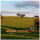
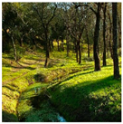
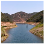
The municipality of Beja, in the Alentejo region of Portugal, with an area of about 1145 km2, was selected for the study (see Figure 1). Different crops characterize this region, but the dominant land use is a mixed agro-silvo-pastoral environment [33,34]. The different agricultural practices require different cropping calendars and field geometries, making the landscape of this region distinctive, with the existence of both fragmented land parcels and larger and more compact ones. This region has a Mediterranean climate, influenced by its distance to the coast (average high temperatures are around 33 °C in August and 14 °C in January) [38]. The mean annual precipitation is around 558 mm, concentrated in the months of November to January. Beja is characterized by a low population density (31 inhabitants per km2). The Guadiana River is the most important watercourse in this region; it crosses the west border of the municipality. The Alqueva Dam was built in 2002 on the Guadiana River, creating the largest artificial lake in Europe. However, it was only fully operational in 2012 in providing water for agriculture services [32].

2.2. Satellite Image Collection and Preprocessing

Landsat data is the longest and most informative temporal report of the earth. It is the only data source that gives a continuous image of the earth’s resources with a high spatial resolution (30 m) spanning nearly 40 years [39]. To obtain vast temporal continuity data and compose our long time series, we downloaded available Landsat data (with less than 50% of cloud cover) from 1995 through 2015 from the official website of the United States Geological Survey (https://earthexplorer.usgs.gov/). This included Landsat 4–5 Level-2 and Landsat 8 Level-2 data (path 203, row 34). We were working with data that spanned 21 years, for a total of 221 scenes (see Table 1). As shown in Table 1, there were no available Landsat images for 2012, either from Landsat 4–5 Level-2 or Landsat 8 Level-2. Only the Landsat 7 sensor had information for 2012, but unfortunately, as is commonly known, all Landsat 7 scenes have data gaps for this area (due to a technical problem with the satellite) [40].
As we were using Landsat Level-2 Surface Reflectance images, no atmospheric correction was needed. Also, no further normalization was required since the TWDTW uses a Generalized Additive Model (GAM) with a spline smooth function and a logistic regression for time weight (see Section 3.4). Furthermore, no masking for clouds or shadows was performed since the TWDTW classifier can “fill in” temporal gaps [17,18]. The ETRS_1989_Portugal_TM06 coordinate system was applied to the image datasets, respecting the 30 x 30 m spatial resolution.

2.3. Official Portuguese Land Cover Map (COS) Data

The COS maps of 1995, 2007, 2010, and 2015 used to derive the training samples were produced by the Portuguese General Directorate for Territorial Development (DGT). These datasets are freely available for download on the DGT website (http://mapas.dgterritorio.pt/geoportal/catalogo.html). The COS maps are in a vector format (polygons) with a cartographic accuracy of 0.5 m and a minimum mapping unit (MMU) of 1 hectare and are produced by photointerpretation (i.e., over orthophoto maps) [41]. COS uses a hierarchical, a priori nomenclature system, having five disaggregation levels. A DGT report [41] describes in detail the COS nomenclature characteristics.

3. Methods

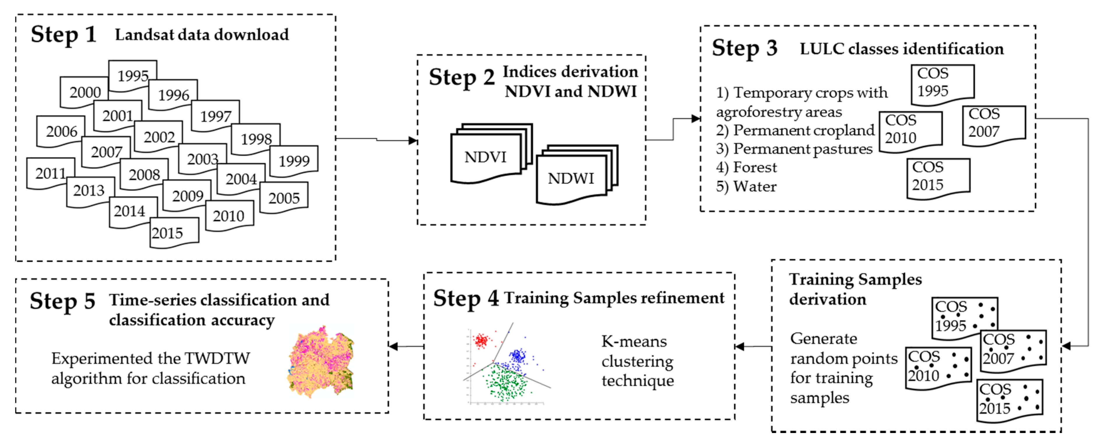
The first step of this research was to download the Landsat Level-2 imagery data from 1995 to 2015. Second, we used the data to compute the normalized difference vegetation index (NDVI) and the normalized difference water index (NDWI). Then, we combined all the scenes to create one raster time-series file for each index. Third, using the COS maps, we identified the most representative LULC classes in the study area and randomly generated sample points for each year to be used in the training. Fourth, we refined the training samples by class and by year using the k-means clustering technique. Finally, in the fifth step, we classified the Landsat imagery time series using the TWDTW algorithm and evaluated the classification accuracy (see Figure 2).

3.1. Derivation of NDVI and NDWI from Landsat Imagery

The municipality of Beja has a heterogeneous biophysical environment, so to improve the identification of the different vegetation classes using Landsat imagery seasonal time series [10,42,43], we computed two indexed time series, NDVI and NDWI. To derive these indices, we used the equations in Table 2.
The normalized difference vegetation index (NDVI) is the most commonly used satellite-based measure to globally monitor vegetation [44] due to its robust and easy interpretation. This index considers the distinctive shape of the vegetation reflectance curve and is able to screen dynamic specifications of vegetation and/or vegetation health [45]. Despite the existence of several other vegetation indices, the ability of the NDVI index to monitor vegetation for seasonal and inter-annual changes has already been sufficiently substantiated in prior studies [44,46]. The normalized difference water index (NDWI) was used as an additional aid, since it was conceived to outline open water features and improve their identification through RS imagery [47,48]. According to Gao [47], this index complements NDVI by improving in the identification of liquid water content of vegetation, whereas NDVI just accounts for the vegetation’s greenness [49].

3.2. Training Sample Derivation

The COS maps for 1995, 2007, 2010, and 2015 were used to produce a sample source for training purposes. As the first step, we statistically analyzed the COS maps to understand what were the main LULC classes in the study area and how they changed over time. The identification of the major LULC classes was based on the second level of nomenclature of the COS maps. We found the predominant temporary crops (51%) in 1995 (Table 3). However, in later years (2007, 2010 and 2015), the coverage of temporary crops declined by almost 8%, though they still represented the largest cropland use (43%). The heterogeneous agricultural areas represented the second largest LULC class over the 21-year period (19% in 1995 and 2015; 20% in 2007 and 2010). Indeed, during this time interval, there was an increase in forested areas (11% in 1995; 12% in 2007; and 13% in 2010 and 2015). Despite the decrease in pasture coverage between 2010 and 2015 by 2%, this LULC class covered about 10% of the study area in 1995 and 12% in 2007. Although permanent crops represent a small amount of LULC in the Beja municipality, they increased substantially (by 7%) between 1995 and 2015. Artificial surfaces and wetlands represent minor LULC classes in this municipality.
The results revealed the predominance of agricultural land (>82%) in the Beja municipality over the 21-year period. Nevertheless, the second largest class (heterogeneous agricultural areas) encompassed different mosaics: (i) areas of temporary crops and/or permanent crops on the same parcel; (ii) temporary crops cultivated under agroforestry systems; (iii) meadows and/or permanent crops, and (iv) landscapes in which crops and pastures intermix with natural vegetation [41]. Indeed, this was a highly heterogeneous class that may include each of the other agricultural classes that predominate in the Beja municipality. When analyzing this class in more detail (looking at the COS maps’ third level of nomenclature), we found a predominance of temporary crops cultivated under agroforestry systems (>85%) over the 21-year period.
Therefore, we decided to mix the temporary crops and the heterogeneous agricultural areas classes. As such, five major LULC classes were identified as the most representative of the selected study area: (1) temporary crops with agroforestry areas (including the temporary crops and the heterogeneous agricultural areas); (2) permanent cropland; (3) permanent pastures; (4) forest; and (5) water. Also, the temporary crops with agroforestry areas could encompass impervious surfaces, since in Beja, the dispersed settlements had relatively small dimensions with houses far apart from each other and surrounded by bare soils and/or croplands. The impervious surfaces were less than 2% of the whole Beja municipality area and have not significantly changed throughout the years.
As the second step, we randomly generated the training sample points for each of the five LULC classes previously identified (see the COS nomenclature codes in Table 4). However, we decided to a priori reduce the polygon areas of the COS maps, using a QGIS Python plugin called “Buffer by Percentage”. We followed this approach, because we knew training samples had low accuracies when their proximity to the polygon’s boundaries increased [50]. As we were using the shape and area of each COS map polygon to produce the training samples, we sought to ensure a relationship of magnitude between the MMUs of both data sources (the COS map and the Landsat imagery) [51]. This ensured the generated samples related to one cell superimposed to just one polygon. Since the COS has an MMU of 1 hectare and the Landsat imagery cell size was 900 m2, we reduced the COS polygon areas to 11% of the original. Consequently, 2000 training samples were generated for the heterogeneous agriculture class (since this area occupied more than 50% of the study area) and 1000 training samples were generated for each of the remaining LULC classes of the four COS maps (1995, 2007, 2010, and 2015) making 6000 samples per year.

3.3. Training Sample Refinement

The created sample source had the following limitations: (1) the sample source was acquired from vector-based LULC data (the COS maps); (2) no training samples acquired from fieldwork were integrated; and (3) there was a high probability of spectral-temporal signature confusion among LULC classes, due to the heterogeneous biophysical environment of the study area. As such, we decided to apply the k-means clustering technique [25,36,37] to improve the sample source.
Cluster analysis methods are normally used in an attempt to detect homogeneous groups. The rationale behind implementing a clustering method to refine the training set is that each generated training sample per class should be grouped to either one or, at most, two clusters. This is due to the fact that each generated training sample should have a similar spectral signature, such as the one belonging to their LULC class. To verify this hypothesis, we used the R package tclust [52].
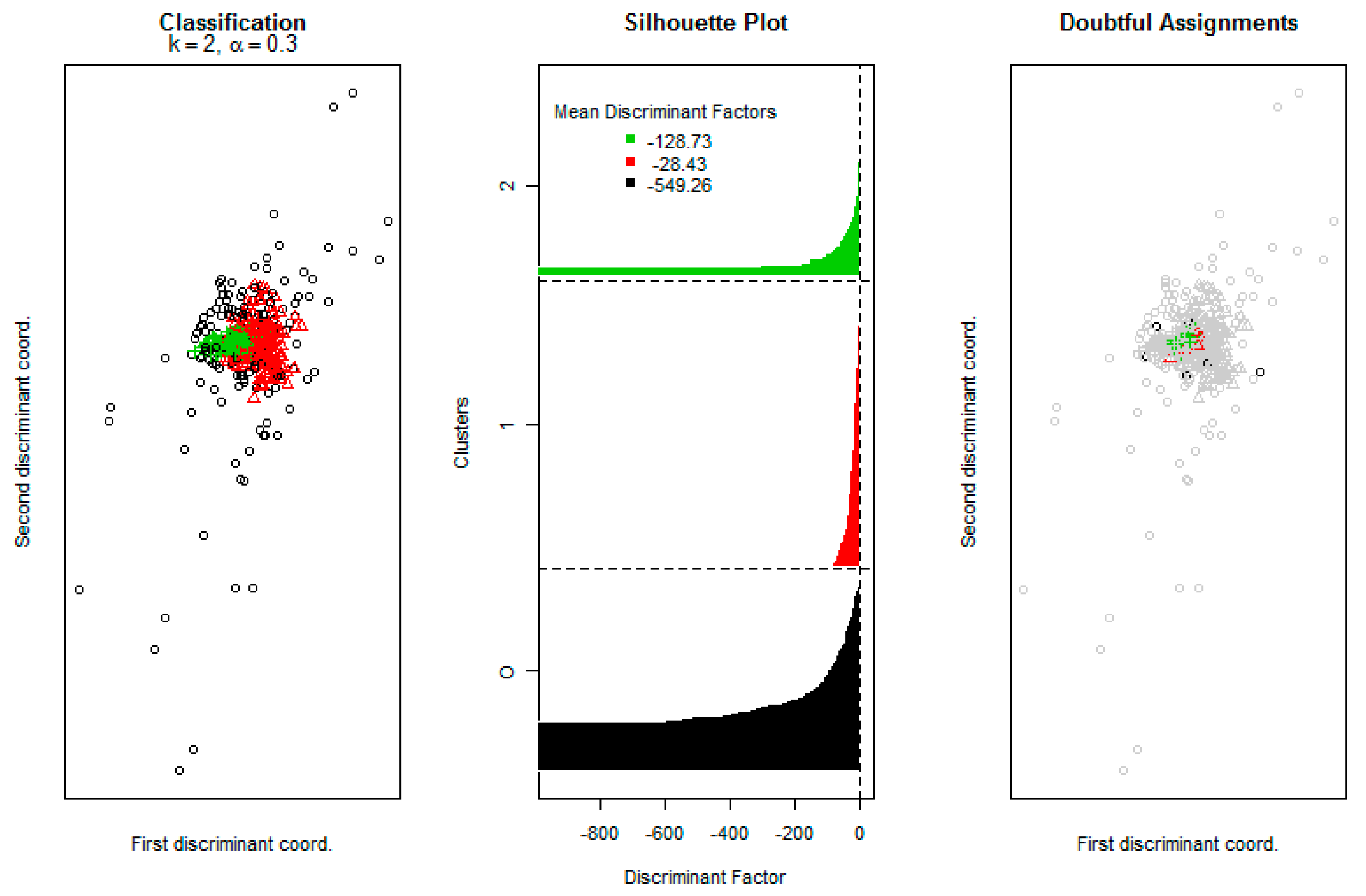
The R package tclust offers an adequate cluster scatter matrix constraint, leading to a wide range of clustering procedures and avoiding the occurrence of spurious non-interesting clusters. Also, it deals with noisy data and provides graphical exploratory tools (see Figure 3) to help the user make sensible choices regarding trimming the outliers and choosing the number of clusters [52]. These options were the main reason why this package was chosen.
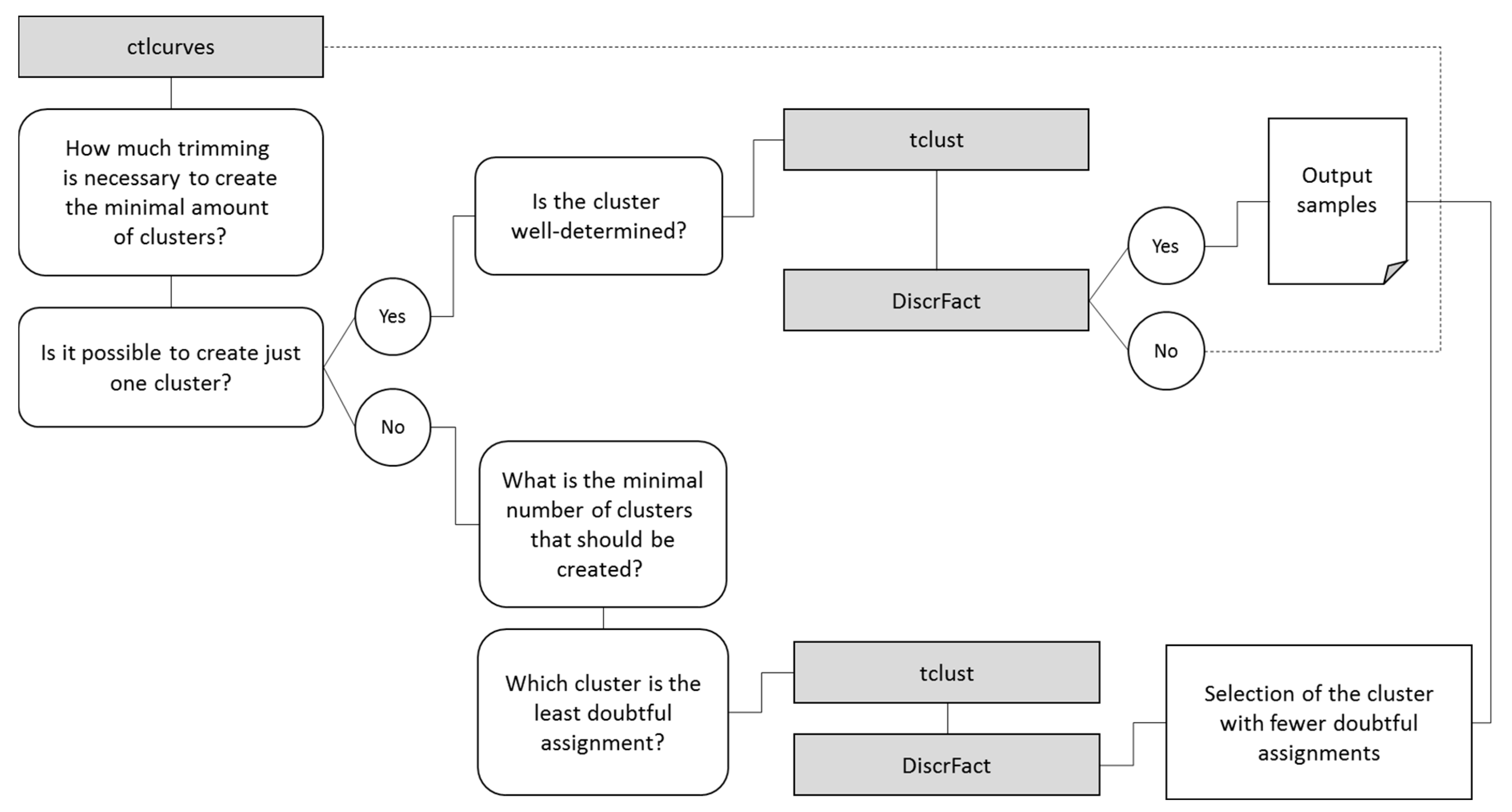
The clustering process is schematically portrayed in Figure 4 and is essentially divided into three distinct processes: (1) classification-trimmed likelihood calculation (ctlcurves); (2) cluster computation; and (3) mean discriminant factor value calculation (DiscrFact). The variables used for the creation of clusters were the NDVI and the NDWI indices (the same variables that would be used for the image classification).
The ctlcurves function approximates the classification-trimmed likelihoods by successively applying the tclust function to a sequence of values, k (number of clusters) and α (fraction of the most outlying data). The calculation of ctlcurves shows the implications of increasing/decreasing k-values in the fraction of the most outlying samples (limited, in this case, to 30% of the sample universe).
To determine the most adequate parameters to include in the tclust function, the following logic was employed:
1. Was it possible to create only one cluster that could well represent each LULC class reality? If so, then only one cluster was created.
2. When more than one cluster had to be created, what was the minimal number of clusters that should be created? In this case, we selected the minimum number of clusters possible, trimming up to the maximum of 30% of the sample universe. When this strategy was put into practice, two and, in rare cases, three clusters were created.
To make sure that in both hypotheses we were left with well-determined clusters, the quality of the cluster assignments and the trimming was evaluated by applying the function DiscrFact. This function helped: (1) to discover if the clusters were well-determined, and (2) to select the cluster with the least doubtful assignments to represent the reality of the respective class [53].
The parameters k and α for the tclust function that provided (among other information) the cluster assignment to each observation, differed according to the results generated by the ctlcurves and DiscrFact functions. The remaining parameters were left at their default values, with the exception of restr that was set to “eigen” to simultaneously control the relative group sizes and the deviation from sphericity in each cluster. Also, the equal.weights parameter was set to “TRUE” to avoid the creation of a well-determined cluster that actually does not represent the LULC class. This way, we achieved heterogeneous clusters as much as possible, since no LULC class had a pure and unique spectral signature. For a correct classification, we needed some variability in the range of values to avoid eliminating potentially important information [52]. The restr.fact parameter was increased until no artificial restriction was necessary to create the clusters [53] (1 being the most restrictive case).
Finally, the tclust package was used to refine the training points generated for each class and for each of the four years. In Table 5, we present the final number of training samples per class for each year after the clustering analysis.

3.4. Dynamic Time Warping and Time-Weighted Dynamic Time Warping Methods

Sakoe and Chiba [54] developed the Dynamic Time Warping (DTW) method for speech recognition applications, and it was later introduced for use in satellite imagery time series analysis [15,16,17,18]. However, DTW proved to be unfit for satellite imagery time-series analysis, because “it disregards the temporal range when trying to find the best pair matches between time series” [21]. The distinctive cycle of each LULC class requires an equilibrium between shape matching and temporal alignment to be employed in LULC classification using remote sensing time-series images [19,20].
To build the time-series analysis, the TWDTW algorithm maps the derived indices (NDVI and NDWI) to a three-dimensional array in space and time, where each pixel location is associated with a sequence of measurements. To match LULC classes to the subintervals (i.e., years) of a long-term satellite image time series and classify phenological cycles, this method uses both cycle amplitude and phase information. The spectral-temporal patterns are defined by applying a GAM [18,21] with a smoothing function of y = s(x), where the function s corresponds to a spline model, x is time, and y is each satellite band.
To set the temporal constraints of the TWDTW algorithm, we applied a logistic weight function, since this provides more accurate results than a linear function [18,21]. This logistic function uses a small weight for short time warps and substantial weight for larger time warps, with a midpoint (beta) and steepness (alpha). It is formally given by (Equation (1)) [18,21]:
w = 1 1 + e α ( g ( t 1 , t 2 ) β )
where g ( t 1 , t 2 ) is the elapsed time (in days) between date t 1 (in the pattern) and date t 2 (in the time series).
The purpose of this function is to control the time warp. If a large seasonal difference exists between the pattern and its matching point in the time series, an additional cost is added to the distance measure (DTW). The g function constraint drives time warping and ensures that the time-series alignment is reliant on the seasons. This is particularly valuable for identifying temporary crops and in differentiating pasture from agriculture. To achieve an LULC classification, and as recommended in Maus et al. [21], we assign the logistic function α = −0.1 and β = 100 to weight the function. This implies adding a time weight to the DTW with a low penalty for time warps smaller than 60 days and a higher penalty for larger time warps. We also set the temporal pattern frequency to eight days to ensure, at least, one Landsat image was considered (i.e., a temporal resolution of eight days).
Since LULC classifications are extremely dependent on the quality of spectro-temporal patterns, we performed a k-fold cross-validation [55]. This function uses the training samples to generate the spectral-temporal patterns. The results of this classification are used in the accuracy calculation. In this study, we obtained the accuracy for each data partition using 100 different data partitions, each of them with 10% of the training samples randomly selected for training and 90% for validation. All calculations and analyses were accomplished using the R programming language and operating environment [56]. Maus et al. [21] implemented the TWDTW method for LULC classifications using satellite imagery time series on an open-source R package (dtwSat, for a package overview see [21]).

3.5. Classification Accuracy Assessment

Several metrics commonly used in remote sensing were calculated, including the kappa index [57], the overall and individual user and producer accuracies [58], the error matrix (confusion matrix), and the confidence intervals for the accuracy measures (error tolerances) [59]. The kappa index estimates how good the classification is when compared to a randomly generated image. The overall accuracy measure indicates total classification performance as a percentage by dividing the number of samples correctly classified by the total number of samples. Individual user accuracy measures the probability that any classified pixel will actually match the samples, while individual producer accuracy provides the probability that a particular LULC class is classified as such in the samples. The error matrix indicates the samples correctly (diagonal) and incorrectly classified for each LULC class.

4. Results

4.1. LULC Classification and Analysis

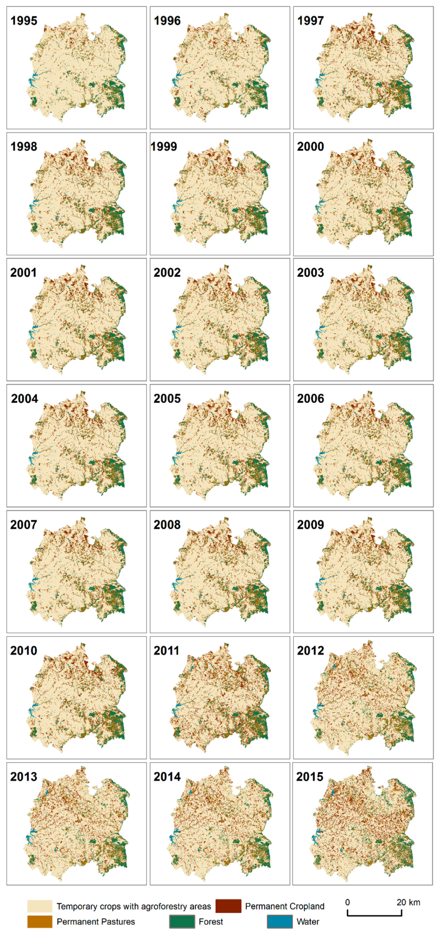
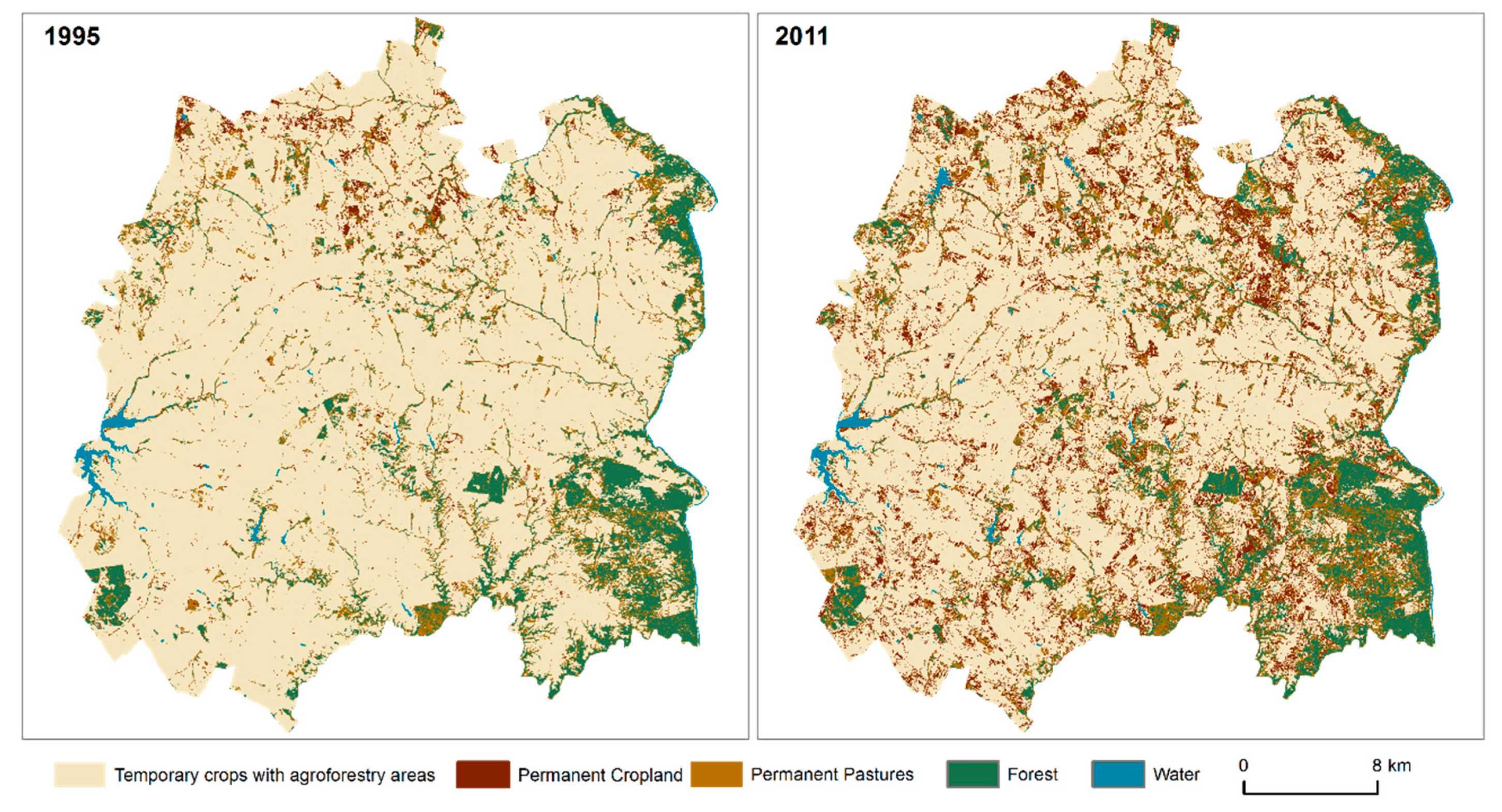
The distance measure is employed to produce categorical land cover maps, where the classification result is based on the most similar pattern for each period. Classification results for each period can be visualized in Figure 5. The results reveal the predominance of temporary crops with agroforestry areas in the Beja municipality. Beja is, in fact, characterized by extensive agriculture with complex cultivation patterns, where significant areas are occupied by temporary crops with natural vegetation and agroforestry areas. The substantial coverage of temporary crops with agroforestry areas confirm the importance of cereal production (particularly wheat) in this municipality, as well as the relevance of cork oak exploitation in the vast landscape of agroforestry areas (named Montado in Portugal and Dehesa in Spain) [34,60].
Over the 21-year period, the biggest change noticed was the substantial increase of the permanent cropland through scattered parcels, especially after the 2010–2011 period. Although this class represents a small coverage in Beja, this considerable increase suggests a change focused on intensive farming without fallow.
We found that permanent pastures represented a minor LULC class and were mainly concentrated near forested areas. Indeed, the forested areas remain mainly in the southeastern and northeastern part of the municipality, possibly due to the topographic conditions (plateaus) and the proximity to the Guadiana River. Figure 6 helps to visualize in detail the main significant changes throughout the 21 years under analysis.
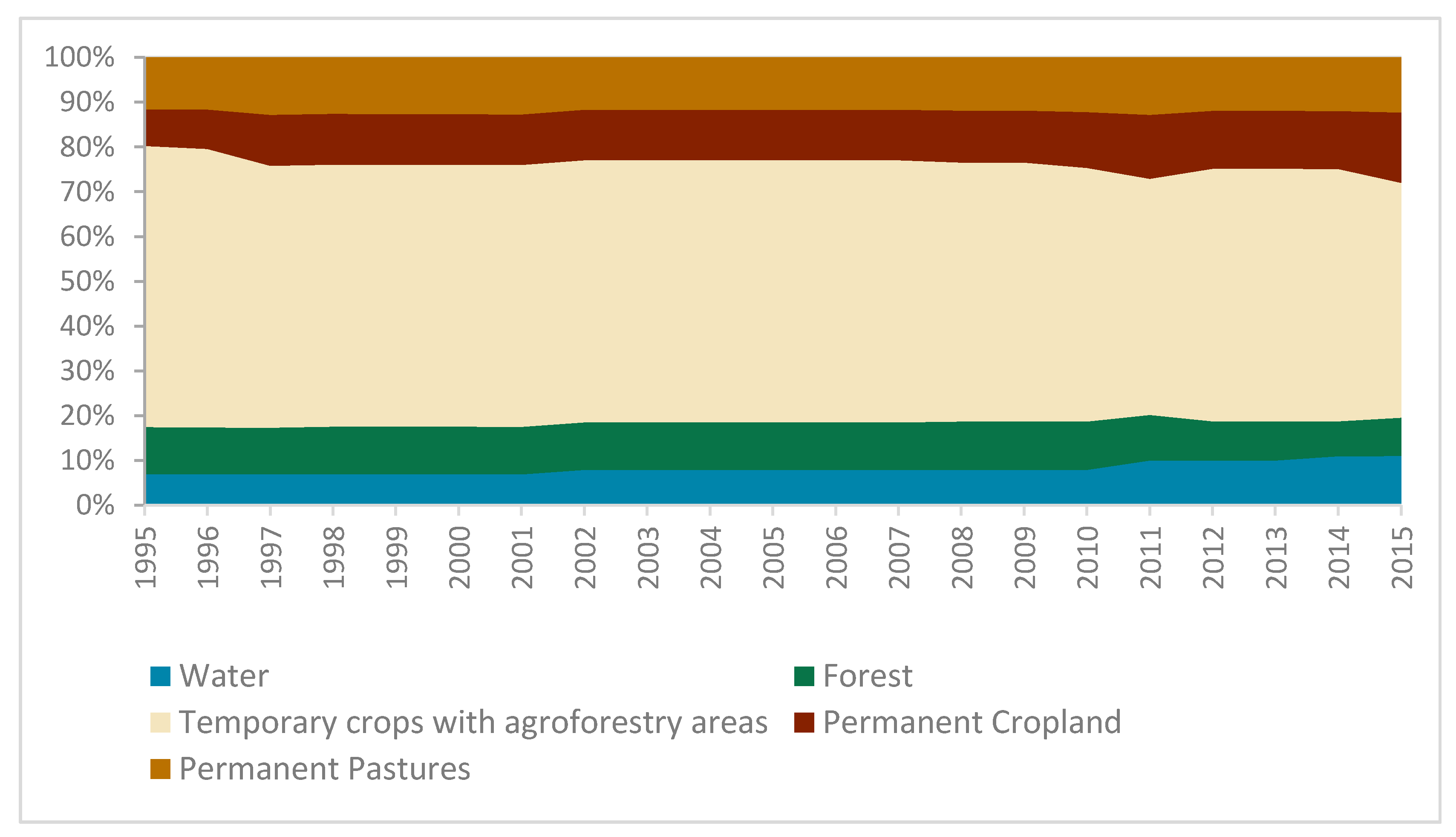
Different occupation areas for each class were observed, which was in agreement with the LULC class spatial distribution. The increase of the permanent cropland was clear from 2011 forward, occupying an area of about 16% in 2015 in contrast with the 1995 occupation area of 8% (Figure 7). The water areas had a similar pattern of consistent increases, up from about 7% of the total area in 1995 to 11% in 2015, with a significant increase in the 2010–2011 period. Regarding the agricultural classes, the temporary crops with agroforestry areas class was clearly prevalent, occupying a total area close to 63% in 1995. However, this class had a significant area decrease from 1995 to 2015 (about 11%). The permanent pastures group did not vary greatly from 1995 to 2015; it always occupied an area of about 12%–13%. Forested areas did vary more over the 21 years analyzed, the area occupied ranged between 11% (maximum area) and 8% (minimum area). In particular, from 2003 to 2010–2011, little or no change in the LULC was detected, perhaps due to the measures brought by the 2003 Common Agriculture Policy (CAP) that more driven by social integration and less to supporting production [32].

4.2. LULC Classification Accuracy Summary

A set of metrics—including overall user and producer accuracy, the kappa index, and an error matrix (confusion matrix) were calculated. The results of the assessment were gathered for the full period (i.e., the total LULC mapping area was the same as the surface area times the number of maps), but it is also possible to evaluate and visualize each period separately. The accuracy assessment was computed using the validation samples (90% of the total samples, with a 95% confidence level), obtaining an overall classification accuracy of 75.96%.
Table 6 presents the error matrix in proportion to the classification map. Only the water class had almost all the samples correctly classified. It is noteworthy that the misclassified samples were mistaken as forest. In this region, forested areas are characterized by hardwood forest that grows along water lines and open spaces with little or no vegetation. Regarding forested areas, there was some confusion between this class and the agricultural classes. Still, only about 4% of the total samples were misclassified. However, between the agricultural classes, the temporary crops with agroforestry areas samples that were misclassified were mostly mistaken as permanent cropland or permanent pastures (about one-quarter of this class’s total sample size). In contrary, the permanent cropland was mostly classified as temporary crops with agroforestry areas (almost 40% of the total sample size was wrongly classified), but it also presented some confusion with the forest class (about 5% of the samples). Similarly, there was some confusion in the permanent pastures class with the temporary crops with agroforestry areas (about 27% of the samples) and also with forest (6% of the samples).
In the class-based analysis, we observed a wide range of accuracy values. The water class was the most accurate, with both use and producer accuracy above 99%, suggesting high confidence and sensitivity of the method for this class. The forest class followed the same pattern as the water class, with high user accuracy (96%) and producer accuracy (88%). However, regarding the agricultural classes, they did not present consistent accuracy values. The temporary crops with agroforestry areas class was the most accurate with a user rate above 74% and a producer rate above 87%, which suggests the pixels classified as temporary crops with agroforestry areas closely matched those in the COS. In contrast, the permanent cropland and permanent pastures classes presented user accuracy values around 56% and 66%, respectively, while the producer accuracy values were even lower (43% for permanent cropland and 39% for permanent pastures). Overall, a kappa coefficient of 0.62 indicated a substantial agreement between the classification and the samples.

5. Discussion

Over the years, the remote sensing applications for rural areas have become extremely important [61], since they support the monitoring and mapping of the LULC changes of agricultural land. Some studies have emphasized the usefulness of using remote sensing data for agricultural land change classification [62,63], cropland estimation/scenario forecast [64,65,66], and vegetation health and crop production monitoring [67,68]. The ongoing abandonment of agricultural land [69,70,71], and the fact that these areas have been threatened by socioeconomic and biophysical factors [72,73] demonstrates the need to identify and characterize the spatiotemporal changes. Accordingly, in this study, we applied a long-term LULC analysis in a rural region based on Landsat time series of 21 years. However, it involved overcoming a number of challenges.

5.1. The Implications of a Long-Term Landsat Time Series

For case studies at a regional scale, Landsat TM/ETM+ has been one of the most frequently used products due to its medium/high spatial resolution (30 m), large temporal extent (since the 1970s), and free and analysis-ready availability [1,2]. However, in this study there were some limitations that were identified regarding the use of the Landsat data.
Having a long time-series span without interruptions was not possible, since there were no images available for the year 2012. Only the Landsat 7 sensor had information relative to 2012, but unfortunately, as is commonly known, many Landsat 7 scenes have data gaps (the result of a technical problem with the satellite) [40]. Although there are several approaches to handling the Landsat 7 sensor error problem, all the processes are time-consuming, and the gaps may not be completely eliminated [74]. In addition, to have a large temporally continuous dataset and create our long time series, we had to combine a set of images of Landsat 4–5 Level-2 and Landsat 8 Level-2 data. As such, the absence of images for 2012 and the use of two different sensors were limitations of this study.
Clouds are often a problem in processing satellite imagery. In our study, the temporal continuity was not affected, as we could use all scenes regardless of the presence of clouds. However, when using other classifiers, a long-term Landsat time series analysis can be difficult, due to the high number of scenes with the presence of clouds, which can affect the temporal continuity and the integrity of the classification.

5.2. The Generation of Training Samples from Official LULC Maps

One challenge associated with a long-term application is the lack of a sufficient and representative training sample. In fact, the accuracy of an image classification result is highly dependent on the quality and quantity of the training set used to train the classification model [75,76]. For most supervised classifiers (such as a maximum likelihood classification, multilayer perceptron, SVM, or RF) not having sufficient and representative training data can be detrimental to the image classification results [24]. Furthermore, in a long-term multitemporal image classification result, it would be very unlikely to have samples for each of the years under study.
Most studies about image classification usually mention the use of field surveys or visual interpretations to obtain training samples [24]. How can a long-term classification be done when both options are not feasible? The approach presented in this study provides a path toward addressing this problem by exploring a way to generate a set of samples for training purposes using free LULC data (the COS maps) from different years. Even if money and time were available to collect training samples from fieldwork, the development of an acceptable automated alternative would allow those resources to be used in other ways.
In this exploratory study, we tested the use of the COS maps to produce a sample source for training purposes for various reasons: (i) the LULC data was produced by a governmental institution (DGT); (ii) it had a medium spatial resolution; (iii) it was the data with most temporal continuity in Portugal; and (iv) it was one of the most used data sources for LULC analysis in Portugal [77]. However, generating training samples from a LULC map (such as the COS) produced by a governmental institution that we considered a reliable source of information still had associated problems. For example, following a previous work [50] we decided to reduce the COS map polygon areas before the generation of random points since the authors of the cited work concluded that the boundaries of the polygons of such sources can have low accuracy. In addition, bias in the representation of the samples can exist if there is no prior knowledge regarding the major LULC types present in the study area. This makes it very difficult to know which LULC classes from the COS should be used to generate the training samples associated with the most representative LULC classes of the study area. We had to support the identification of the major LULC classes present in our study area by a statistical analysis of the coverage of the COS LULC classes.
In addition, even though we were able to generate 6000 training samples for each year in the study, this set was irregularly distributed over time, since it only represented the information of the LULC for four of the 21 years under analysis. This was, in fact, the major constraint we had, and, once again, it depicted the limitations associated with this type of remote sensing application.

5.3. The LULC Types and Temporal Phenological Signatures Diversity

In our study, we decided to apply the k-means clustering technique to refine the training samples, since they were acquired using an explorative approach without integrating any ground-truth data and there was mixed agro-silvo-pastoral ecosystem present in our study area. Moreover, Viana et al. [37] had already demonstrated the training samples refinement using the k-means clustering technique improves the image classification’s overall accuracy (+8%).
Interestingly, Allen et al. [32] and Senf et al. [78] had already mentioned the difficulty of classifying the different LULC types of a region with a heterogeneous biophysical environment due to the wide range of spectral signatures for each LULC class. Our word with the Beja municipal region was no different; the permanent cropland class is an example of a class with a complex spectral pattern. This class was mostly constituted of olive groves, and the production techniques of olive groves have changed over the past decade. This region has always been characterized by open olive grove crops, but recent foreign direct investment in super-intensive olive grove plantations has resulted in a different landscape. It is easy to find intensive and super-intensive olive grove production, which is a particular type with its own spectral signature characteristics that differ from the “usual” open olive grove production (since the trees are small, have less space between them, and have no grass beneath). As such, the same LULC class can have different spectral signatures, which helps explain the low accuracy values for the permanent cropland class and the confusion between the remaining agricultural classes.
As mentioned before, the Beja municipality has a heterogeneous land cover area (with the existence of both fragmented parcels and larger and compact parcels) with different crop phenological cycles and agricultural practices. In addition, the most misclassification was between the permanent cropland and temporary crops with agroforestry areas presumably due to how olive groves (when not super-intensively produced) and especially the vineyard planting was organized (in line with spaces of bare soil between them). Also, the presence and extent of Montado in the Beja municipality can easily explain the misclassification among each of the three agricultural classes, since this class is mostly characterized by a herbaceous understory, and can, therefore, be easily mistaken with olive groves or pastures [32].
In particular, Allen et al. [32] have emphasized the lack of research focusing on the detection of LULC changes in the Alentejo region, based on identifying the extent of more than one type of LULC at a large temporal scale. The approaches of Calvão and Palmeirim [79] and Godinho et al. [60] to identify the LULC changes in Alentejo were focused on single classes (semi-deciduous scrub, and Montado, respectively). As a matter of fact, Allen et al. [32] were the first to assess the extent of the changes in the different LULC classes present in an agro-silvo-pastoral environment and recognized the limitations of such analysis. Our study reveals similar drawbacks that emerged in the classification confusion among the agricultural classes present in our study area.
Nevertheless, the final result is a starting point for understanding the LULC dynamics for 21 years—confirming the impact some political decisions have had in this region (such as the construction of the Alqueva Dam in 2002 that filled its reservoir until 2012) and the lack of control of the type of agricultural activity that has had a significant impact on soil quality due to the super-intensive production for permanent crops like the case of the olive groves.

5.4. The TWDTW Method for Long-Term Time-Series Classification

This study also introduced the use of the TWDTW method for long-term classification using the Landsat time series. The TWDTW had already successfully achieved high accuracy values for satellite time series, using MODIS imagery [18,21] and Sentinel-2 imagery [22], showing to a certain extent the capacity of this classifier for handling multidimensional analysis. In this study, the assessment revealed an overall good accuracy of about 76%. Although the water and forest classes had contributed to this overall value, the accuracy values obtained for each of the three agricultural classes (the agricultural classes were prevalent in the study area, occupying about 80% of the total area) were problematic. Certainly, the 24% misclassification rate among the LULC classes could have a statistical influence in the results, particularly in relation to the extent of the changes in classes over the 21-year period. However, our results are in accordance with the statistical analysis we performed with the COS maps (Section 3.2), which allowed identifying the main LULC classes in the study area and how they changed over time.
It is noteworthy that this misclassification among each of the three agricultural classes was already expected, due to the complex spectral properties of the different vegetation types present in these large agricultural classes. This is especially true for temporary crops with agroforestry areas. They have a complex cultivation pattern encompassing temporary irrigated and rain-fed crops that are produced and harvested in different seasons followed by bare soil afterwards that can be easily confused with the permanent cropland and permanent pastures. Furthermore, the classifications are complicated by the more recent super-intensive production for permanent crops like the case of the olive groves [80]. Intensification of the permanent cropland is very likely associated with increased exploitation of water resources, following the construction of Alqueva Dam. The increased expansion of water bodies is also apparently attributable to the construction of this Dam [32].
In addition, to improve the identification of each LULC type and increase the classification accuracy, we decided to compute two-time series indices (NDVI and NDWI) and perform the cluster analysis using the spectral signatures of the training samples for all LULC classes. However, we recognize that there may be other indices that can be used to further improve the results, such as the enhanced vegetation index (EVI) [17,63,68], the generalized soil adjusted vegetation index (SAVI) [81], or the Modified Soil-adjusted Vegetation Index (MSAVI) [82]. These should be considered in further studies.
Nevertheless, our results, in line with Maus et al. [18], and Belgiu and Csillik [22], highlight the potential of this method to classify complex ecosystems, especially if we take into account our methodology’s major constraint, the sample set irregularly distributed over time. Yet, it is important to highlight the processing time associated to create the categorical LULC map for each period when using the dtwSat package. The TWDTW method processing time (using an Intel® Core™ i7-6700K CPU with a 4.00 GHz clock and 32 GB of RAM) was almost 16 hours when processing in parallel [21]. This can be an issue to take into account, especially if we want to reproduce this approach for larger areas or if the available hardware has limited resources.

6. Conclusions

In this study, the TWDTW method was used to classify a heterogeneous area located in the southeast of Portugal, providing insights into the main changes that occurred over 21 years. This time series, derived from Landsat data, facilitated the inter-annual change comparisons in cropland type activity in an area of predominantly mixed cropland. If we consider the above-mentioned limitations (absence of images for 2012, the use of two different satellite sensors, and the training samples irregularly distributed over time) and the overall good classification accuracy value obtained, we are truly convinced that in the near future, this classifier will become one of the most used for time-series classification, especially because it is an open-source and free method for remote sensing time-series analysis.
The cluster analysis performed on R was efficient and straightforward. It proved itself a promising approach capable of detecting homogeneous training sample groups for each class. It guaranteed an acceptable level of quality, as we collected the samples based on vector cartography, the polygons constituted homogeneous entities, and the salt-and-pepper effect proliferated in the satellite images.
Also, we acknowledge that with the COS data we could have already had a notion of the major transformations, but we would not have had seen the trends from year to year and been able to quantify them. In addition, the time gap of the COS data was very large, especially between the first and the second maps (12 years apart). Also, this methodology can now be replicated for other study areas, using other LULC data (such as CORINE Land Cover (CLC), since it is available for most of Europe and for the years 1990, 2000, 2006, 2012, and 2018). Also, for more recent years, the OpenStreetMap data can be a reliable alternative since this source of voluntary geographic information has a level of accuracy similar to the COS.
For future studies, it would be important to try to disaggregate the three major agricultural classes into subclasses to make it possible to describe the type of crop in detail. Ultimately, we conducted a study, using only open data and open software that has allowed gaining more insight regarding a relatively large rural area (>1000 km2). It is an area where the LULC changes have been dynamic, and the data provide support to improve cropland management with sustainable practices and policies.

Author Contributions

Conceptualization, C.M.V. and J.R.; methodology & software, C.M.V., I.G. and J.R.; data curation, C.M.V and I.G.; validation, C.M.V. and J.R.; formal analysis, C.M.V.; investigation, C.M.V.; writing—original draft preparation, C.M.V; writing—review and editing, C.M.V.

Funding

This research was funded by FCT - Portuguese Foundation for Science and Technology [grant number SFRH/BD/115497/2016 to Cláudia M. Viana and grant number SFRH/BD/138979/2018 to Inês Girão].

Acknowledgments

We acknowledge the GEOMODLAB - Laboratory for Remote Sensing, Geographical Analysis and Modelling—of the Center of Geographical Studies/IGOT for providing the required equipment and software, the publication financing by Centre for Geographical Studies—Universidade de Lisboa and FCT [UID/GEO/00295/2013], and the five anonymou14s reviewers that contributed to the improvement of this paper.

Conflicts of Interest

The authors declare no conflict of interest.

References

  1. Hansen, M.C.; Loveland, T.R. A review of large area monitoring of land cover change using Landsat data. Remote Sens. Environ. 2012, 122, 66–74. [Google Scholar] [CrossRef]
  2. Wulder, M.A.; Masek, J.G.; Cohen, W.B.; Loveland, T.R.; Woodcock, C.E. Opening the archive: How free data has enabled the science and monitoring promise of Landsat. Remote Sens. Environ. 2012, 122, 2–10. [Google Scholar] [CrossRef]
  3. Lunetta, R.S.; Knight, J.F.; Ediriwickrema, J.; Lyon, J.G.; Worthy, L.D. Land-cover change detection using multi-temporal MODIS NDVI data. Remote Sens. Environ. 2006, 105, 142–154. [Google Scholar] [CrossRef]
  4. Xiao, X.; Boles, S.; Liu, J.; Zhuang, D.; Frolking, S.; Li, C.; Salas, W.; Moore, B. Mapping paddy rice agriculture in southern China using multi-temporal MODIS images. Remote Sens. Environ. 2005, 95, 480–492. [Google Scholar] [CrossRef]
  5. Schmidt, M.; Lucas, R.; Bunting, P.; Verbesselt, J.; Armston, J. Multi-resolution time series imagery for forest disturbance and regrowth monitoring in Queensland, Australia. Remote Sens. Environ. 2015, 158, 156–168. [Google Scholar] [CrossRef] [Green Version]
  6. Zhu, Z.; Woodcock, C.E. Continuous change detection and classification of land cover using all available Landsat data. Remote Sens. Environ. 2014, 144, 152–171. [Google Scholar] [CrossRef]
  7. Yan, L.; Roy, D.P. Improved time series land cover classification by missing-observation-adaptive nonlinear dimensionality reduction. Remote Sens. Environ. 2015, 158, 478–491. [Google Scholar] [CrossRef] [Green Version]
  8. Gómez, C.; White, J.C.; Wulder, M.A. Optical remotely sensed time series data for land cover classification: A review. ISPRS J. Photogramm. Remote Sens. 2016, 116, 55–72. [Google Scholar] [CrossRef] [Green Version]
  9. Khatami, R.; Mountrakis, G.; Stehman, S.V. A meta-analysis of remote sensing research on supervised pixel-based land-cover image classification processes: General guidelines for practitioners and future research. Remote Sens. Environ. 2016, 177, 89–100. [Google Scholar] [CrossRef] [Green Version]
  10. Carrão, H.; Gonçalves, P.; Caetano, M. Contribution of multispectral and multitemporal information from MODIS images to land cover classification. Remote Sens. Environ. 2008, 112, 986–997. [Google Scholar] [CrossRef]
  11. Rufin, P.; Müller, H.; Pflugmacher, D.; Hostert, P. Land use intensity trajectories on Amazonian pastures derived from Landsat time series. Int. J. Appl. Earth Obs. Geoinf. 2015, 41, 1–10. [Google Scholar] [CrossRef]
  12. Seto, K.C.; Fragkias, M. Quantifying spatiotemporal patterns of urban land-use change in four cities of China with time series landscape metrics. Landsc. Ecol. 2005, 20, 871–888. [Google Scholar] [CrossRef]
  13. Phiri, D.; Morgenroth, J. Developments in Landsat land cover classification methods: A review. Remote Sens. 2017, 9, 967. [Google Scholar] [CrossRef]
  14. Raczko, E.; Zagajewski, B. Comparison of support vector machine, random forest and neural network classifiers for tree species classification on airborne hyperspectral APEX images. Eur. J. Remote Sens. 2017, 50, 144–154. [Google Scholar] [CrossRef]
  15. Petitjean, F.; Inglada, J.; Gancarski, P. Satellite Image Time Series Analysis Under Time Warping. IEEE Trans. Geosci. Remote Sens. 2012, 50, 3081–3095. [Google Scholar] [CrossRef]
  16. Petitjean, F.; Weber, J. Efficient Satellite Image Time Series Analysis Under Time Warping. IEEE Geosci. Remote Sens. Lett. 2014, 11, 1143–1147. [Google Scholar] [CrossRef]
  17. Guan, X.; Huang, C.; Liu, G.; Meng, X.; Liu, Q. Mapping rice cropping systems in Vietnam using an NDVI-based time-series similarity measurement based on DTW distance. Remote Sens. 2016, 8, 19. [Google Scholar] [CrossRef]
  18. Maus, V.; Camara, G.; Cartaxo, R.; Sanchez, A.; Ramos, F.M.; Ribeiro, G.Q. A Time—Weighted Dynamic Time Warping Method for Land-Use and Land-Cover Mapping. IEEE J. Sel. Top. Appl. Earth Obs. Remote Sens. 2016, 9, 3729–3739. [Google Scholar] [CrossRef]
  19. Reed, B.C.; Brown, J.F.; VanderZee, D.; Loveland, T.R.; Merchant, J.W.; Ohlen, D.O. Measuring phenological variability from satellite imagery. J. Veg. Sci. 1994, 5, 703–714. [Google Scholar] [CrossRef]
  20. Zhang, X.; Friedl, M.A.; Schaaf, C.B.; Strahler, A.H.; Hodges, J.C.F.; Gao, F.; Reed, B.C.; Huete, A. Monitoring vegetation phenology using MODIS. Remote Sens. Environ. 2003, 84, 471–475. [Google Scholar] [CrossRef]
  21. Maus, V.; Câmara, G.; Appel, M.; Pebesma, E. dtwSat: Time-Weighted Dynamic Time Warping for Satellite Image Time Series Analysis in R. J. Stat. Softw. 2019, 88, 1–31. [Google Scholar] [CrossRef]
  22. Belgiu, M.; Csillik, O. Sentinel-2 cropland mapping using pixel-based and object-based time-weighted dynamic time warping analysis. Remote Sens. Environ. 2018, 204, 509–523. [Google Scholar] [CrossRef]
  23. Csillik, O.; Belgiu, M. Cropland mapping from Sentinel-2 time series data using object-based image analysis. In Proceedings of the 20th AGILE International Conference on Geographic Information Science, Wageningen, The Netherlands, 9–12 May 2017. [Google Scholar]
  24. Lu, D.; Weng, Q. A survey of image classification methods and techniques for improving classification performance. Int. J. Remote Sens. 2007, 28, 823–870. [Google Scholar] [CrossRef] [Green Version]
  25. Usman, B. Satellite Imagery Land Cover Classification using K-Means Clustering Algorithm Computer Vision for Environmental Information Extraction. Sci. Eng. 2013, 63, 18671–18675. [Google Scholar] [CrossRef]
  26. Lu, Q.; Ma, Y.; Xia, G.S. Active learning for training sample selection in remote sensing image classification using spatial information. Remote Sens. Lett. 2017, 8, 1210–1219. [Google Scholar] [CrossRef]
  27. Huang, X.; Weng, C.; Lu, Q.; Feng, T.; Zhang, L. Automatic labelling and selection of training samples for high-resolution remote sensing image classification over urban areas. Remote Sens. 2015, 7, 16024–16044. [Google Scholar] [CrossRef]
  28. EEA. Down to Earth: Soil Degradation and Sustainable Development in Europe. A Challenge for the 21st Century; European Environment Agency (EEA): Copenhagen, Denmark, 2000. [Google Scholar]
  29. FAO. The State of Food Insecurity in the World: Addressing Food Insecurity in Protracted Crises; FAO: Rome, Italy, 2010; ISBN 9789251066102. [Google Scholar]
  30. Baessler, C.; Klotz, S. Effects of changes in agricultural land-use on landscape structure and arable weed vegetation over the last 50 years. Agric. Ecosyst. Environ. 2006, 115, 43–50. [Google Scholar] [CrossRef]
  31. Noszczyk, T.; Rutkowska, A.; Hernik, J. Exploring the land use changes in Eastern Poland: Statistics-based modeling. Hum. Ecol. Risk Assess. 2019, 1–28. [Google Scholar] [CrossRef]
  32. Allen, H.; Simonson, W.; Parham, E.; Santos, E.d.B.E.; Hotham, P. Satellite remote sensing of land cover change in a mixed agro-silvo-pastoral landscape in the Alentejo, Portugal. Int. J. Remote Sens. 2018, 1–21. [Google Scholar] [CrossRef]
  33. Russo, R.O. Agrosilvopastoral Systems: A Practical Approach Toward Sustainable Agriculture. J. Sustain. Agric. 1996, 7, 5–16. [Google Scholar] [CrossRef]
  34. Correia, T.P. Threatened landscape in Alentejo, Portugal: The ‘montado’ and other ‘agro-silvo-pastoral’ systems. Landsc. Urban Plan. 1993, 24, 43–48. [Google Scholar] [CrossRef]
  35. Godinho, S.; Guiomar, N.; Machado, R.; Santos, P.; Sá-Sousa, P.; Fernandes, J.P.; Neves, N.; Pinto-Correia, T. Assessment of environment, land management, and spatial variables on recent changes in montado land cover in southern Portugal. Agrofor. Syst. 2016, 90, 177–192. [Google Scholar] [CrossRef]
  36. Cuesta-Albertos, J.A.; Gordaliza, A.; Matrán, C. Trimmed k-means: An attempt to robustify quantizers. Ann. Stat. 1997, 25, 553–576. [Google Scholar] [CrossRef]
  37. Viana, C.M.; Girão, I.; Rocha, J. Training samples from open data for satellite imagery classification: Using K-means clustering algorithm. In Proceedings of the 22nd AGILE Conference on Geo-Information Science, Limassol, Cyprus, 17–20 June 2019. [Google Scholar]
  38. Instituto Português do Mar e da Atmosfera (IPMA). Iberian Climate Atlas. Available online: http://www.ipma.pt/resources.www/docs_pontuais/ocorrencias/2011/atlas_clima_iberico.pdf (accessed on 10 January 2019).
  39. Woodcock, C.E.; Allen, R.; Anderson, M.; Belward, A.; Bindschadler, R.; Cohen, W.; Gao, F.; Goward, S.N.; Helder, D.; Helmer, E.; et al. Free Access to Landsat Imagery. Science 2008, 320, 1011a. [Google Scholar] [CrossRef]
  40. Hossain, M.S.; Bujang, J.S.; Zakaria, M.H.; Hashim, M. Assessment of the impact of Landsat 7 Scan Line Corrector data gaps on Sungai Pulai Estuary seagrass mapping. Appl. Geomat. 2015, 7, 189–202. [Google Scholar] [CrossRef]
  41. DGT. Especificações Técnicas da Carta de Uso e Ocupação do Solo (COS) de Portugal Continental para 1995, 2007, 2010 e 2015; Lisboa. 2018. Available online: http://mapas.dgterritorio.pt/atom-dgt/pdf-cous/COS2015/ET-COS-1995-2007-2010-2015.pdf (accessed on 10 January 2019).
  42. Lobo, A.; Legendre, P.; Rebollar, J.L.G.; Carreras, J.; Ninot, J.M. Land cover classification at a regional scale in Iberia: Separability in a multi-temporal and multi-spectral data set of satellite images. Int. J. Remote Sens. 2004, 25, 205–213. [Google Scholar] [CrossRef]
  43. Vicente-Serrano, S.M.; Heredia-Laclaustra, A. NAO influence on NDVI trends in the Iberian peninsula (1982–2000). Int. J. Remote Sens. 2004, 25, 2871–2879. [Google Scholar] [CrossRef]
  44. Rouse, J.W.; Hass, R.H.; Schell, J.A.; Deering, D.W. Monitoring vegetation systems in the great plains with ERTS. Third Earth Resour. Technol. Satell. Symp. 1973, 1, 309–317. [Google Scholar]
  45. Azzali, S.; Menenti, M. Mapping vegetation-soil-climate complexes in southern Africa using temporal Fourier analysis of NOAA-AVHRR NDVI data. Int. J. Remote Sens. 2000, 21, 973–996. [Google Scholar] [CrossRef]
  46. Yuan, F.; Bauer, M.E. Comparison of impervious surface area and normalized difference vegetation index as indicators of surface urban heat island effects in Landsat imagery. Remote Sens. Environ. 2007, 106, 375–386. [Google Scholar] [CrossRef]
  47. Gao, B.C. NDWI—A normalized difference water index for remote sensing of vegetation liquid water from space. Remote Sens. Environ. 1996, 58, 257–266. [Google Scholar] [CrossRef]
  48. McFeeters, S.K. The use of the Normalized Difference Water Index (NDWI) in the delineation of open water features. Int. J. Remote Sens. 1996, 17, 1425–1432. [Google Scholar] [CrossRef]
  49. Ceccato, P.; Gobron, N.; Flasse, S.; Pinty, B.; Tarantola, S. Designing a spectral index to estimate vegetation water content from remote sensing data: Part 2. Validation and applications. Remote Sens. Environ. 2002, 82, 198–207. [Google Scholar] [CrossRef]
  50. Viana, C.M.; Encalada, L.; Rocha, J. The value of OpenStreetMap Historical Contributions as a Source of Sampling Data for Multi-temporal Land Use/Cover Maps. Isprs Int. J. Geo-Inf. 2019, 8, 116. [Google Scholar] [CrossRef]
  51. García-Álvarez, D. The Influence of Scale in LULC Modeling. A Comparison Between Two Different LULC Maps (SIOSE and CORINE). In Geomatic Simulations and Scenarios for Modelling LUCC. A Review and Comparison of Modelling Techniques; Camacho Olmedo, M.T., Paegelow, M., Mas, J.F., Escobar, F., Eds.; Springer: Cham, Switzerland, 2018; pp. 187–213. [Google Scholar]
  52. Fritz, H.; García-Escudero, L.A.; Mayo-Iscar, A. tclust: An R Package for a Trimming Approach to Cluster Analysis. J. Stat. Softw. 2012, 47. [Google Scholar] [CrossRef]
  53. Rousseeuw, P.J. Silhouettes: A graphical aid to the interpretation and validation of cluster analysis. J. Comput. Appl. Math. 1987, 20, 53–65. [Google Scholar] [CrossRef] [Green Version]
  54. Sakoe, H.; Chiba, S. Dynamic Programming Algorithm Optimization for Spoken Word Recognition. IEEE Trans. Acoust. 1978, 26, 43–49. [Google Scholar] [CrossRef]
  55. Ramezan, C.A.; Warner, T.A.; Maxwell, A.E. Evaluation of Sampling and Cross-Validation Tuning Strategies for Regional-Scale Machine Learning Classification. Remote Sens. 2019, 11, 185. [Google Scholar] [CrossRef]
  56. R Core Team. R: A Language and Environment for Statistical Computing; R Foundation for Statistical Computing: Vienna, Austria, 2017. [Google Scholar]
  57. Landis, J.R.; Koch, G.G. The Measurement of Observer Agreement for Categorical Data. Biometrics 1977, 33, 159–174. [Google Scholar] [CrossRef]
  58. Jokar Arsanjani, J.; Mooney, P.; Zipf, A.; Schauss, A. Quality Assessment of the Contributed Land Use Information from OpenStreetMap Versus Authoritative Datasets; Springer: Cham, Switzerland, 2015; pp. 37–58. [Google Scholar]
  59. Baraldi, A.; Puzzolo, V.; Blonda, P.; Bruzzone, L.; Tarantino, C. Automatic spectral rule-based preliminary mapping of calibrated landsat TM and ETM+ images. IEEE Trans. Geosci. Remote Sens. 2006, 44, 2563–2585. [Google Scholar] [CrossRef]
  60. Godinho, S.; Gil, A.; Guiomar, N.; Neves, N.; Pinto-Correia, T. A remote sensing-based approach to estimating montado canopy density using the FCD model: A contribution to identifying HNV farmlands in southern Portugal. Agrofor. Syst. 2016, 90, 23–34. [Google Scholar] [CrossRef]
  61. Atzberger, C. Advances in remote sensing of agriculture: Context description, existing operational monitoring systems and major information needs. Remote Sens. 2013, 5, 949–981. [Google Scholar] [CrossRef]
  62. Ross, C.; Fildes, S.; Millington, A. Land-Use and Land-Cover Change in the Páramo of South-Central Ecuador, 1979–2014. Land 2017, 6, 46. [Google Scholar] [CrossRef]
  63. Wardlow, B.D.; Egbert, S.L.; Kastens, J.H. Analysis of time-series MODIS 250 m vegetation index data for crop classification in the U.S. Central Great Plains. Remote Sens. Environ. 2007, 108, 290–310. [Google Scholar] [CrossRef] [Green Version]
  64. Lyle, G.; Lewis, M.; Ostendorf, B. Testing the temporal ability of landsat imagery and precision agriculture technology to provide high resolution historical estimates of wheat yield at the farm scale. Remote Sens. 2013, 5, 1549–1567. [Google Scholar] [CrossRef]
  65. Mulianga, B.; Bégué, A.; Simoes, M.; Todoroff, P. Forecasting regional sugarcane yield based on time integral and spatial aggregation of MODIS NDVI. Remote Sens. 2013, 5, 2184–2199. [Google Scholar] [CrossRef]
  66. Meroni, M.; Marinho, E.; Sghaier, N.; Verstrate, M.M.; Leo, O. Remote sensing based yield estimation in a stochastic framework—Case study of durum wheat in Tunisia. Remote Sens. 2013, 5, 539–557. [Google Scholar] [CrossRef]
  67. Gumma, M.K.; Thenkabail, P.S.; Teluguntla, P.; Rao, M.N.; Mohammed, I.A.; Whitbread, A.M. Mapping rice-fallow cropland areas for short-season grain legumes intensification in South Asia using MODIS 250 m time-series data. Int. J. Digit. Earth 2016, 9, 981–1003. [Google Scholar] [CrossRef]
  68. Teluguntla, P.; Ryu, D.; George, B.; Walker, J.; Malano, H. Mapping Flooded Rice Paddies Using Time Series of MODIS Imagery in the Krishna River Basin, India. Remote Sens. 2015, 7, 8858–8882. [Google Scholar] [CrossRef] [Green Version]
  69. Radwan, T.M.; Blackburn, G.A.; Whyatt, J.D.; Atkinson, P.M. Dramatic Loss of Agricultural Land Due to Urban Expansion Threatens Food Security in the Nile Delta, Egypt. Remote Sens. 2019, 11, 332. [Google Scholar] [CrossRef]
  70. Shi, K.; Chen, Y.; Yu, B.; Xu, T.; Li, L.; Huang, C.; Liu, R.; Chen, Z.; Wu, J. Urban expansion and agricultural land loss in China: A multiscale perspective. Sustainability 2016, 8, 790. [Google Scholar] [CrossRef]
  71. Fuchs, R.; Herold, M.; Verburg, P.H.; Clevers, J.G.P.W.; Eberle, J. Gross changes in reconstructions of historic land cover/use for Europe between 1900 and 2010. Glob. Chang. Biol. 2015, 21, 299–313. [Google Scholar] [CrossRef]
  72. Serra, P.; Pons, X.; Saurí, D. Land-cover and land-use change in a Mediterranean landscape: A spatial analysis of driving forces integrating biophysical and human factors. Appl. Geogr. 2008, 28, 189–209. [Google Scholar] [CrossRef]
  73. Feranec, J.; Soukup, T.; Taff, G.; Stych, P.; Bicik, I. Overview of changes in land cover and land use in Eastern Europe. In Land-Cover and Land-Use Changes in Eastern Europe after the Collapse of the Soviet Union in 1991; Gutman, G., Radeloff, V., Eds.; Springer: Berlin/Heidelberg, Germany, 2017. [Google Scholar]
  74. Simoes, R.E.O.; Pletsch, M.A.J.S.; Santos, L.A.; Câmara, G.; Maus, V. Satellite Multisensor Spatiotemporal Analysis: A TWDTW Preview Approach. 2017. Available online: https://proceedings.science/sbsr/papers/satellite-multisensor-spatiotemporal-analysis--a-twdtw-preview-approach?lang=pt-br (accessed on 1 January 2019).
  75. Lippitt, C.D.; Rogan, J.; Li, Z.; Eastman, J.R.; Jones, T.G. Mapping Selective Logging in Mixed Deciduous Forest: A Comparison of Machine Learning Algorithms. Photogramm. Eng. Remote Sens. 2008, 74, 1201–1211. [Google Scholar] [CrossRef]
  76. Brodley, C.E.; Friedl, M.A. Identifying Mislabeled Training Data. J. Artif. Intell. Res. 1999, 131–167. [Google Scholar] [CrossRef]
  77. Meneses, B.M.; Reis, E.; Vale, M.J.; Reis, R. Modelling the Land Use and Land cover changes in Portugal: A multi-scale and multi-temporal approach. Finisterra 2018, 53. [Google Scholar] [CrossRef]
  78. Senf, C.; Leitão, P.J.; Pflugmacher, D.; van der Linden, S.; Hostert, P. Mapping land cover in complex Mediterranean landscapes using Landsat: Improved classification accuracies from integrating multi-seasonal and synthetic imagery. Remote Sens. Environ. 2015, 156, 527–536. [Google Scholar] [CrossRef]
  79. Calvão, T.; Palmeirim, J.M. A comparative evaluation of spectral vegetation indices for the estimation of biophysical characteristics of mediterranean semi-deciduous shrub communities. Int. J. Remote Sens. 2011, 32, 2275–2296. [Google Scholar] [CrossRef]
  80. Viana, C.M.; Rocha, J. Spatiotemporal analysis and scenario simulation of agricultural land use land cover using GIS and a Markov chain model. In Geospatial Technologies for All: Short Papers, Posters and Poster Abstracts of the 21th AGILE Conference on Geographic Information Science; Mansourian, A., Pilesjö, P., Harrie, L., von Lammeren, R., Eds.; Lund University: Lund, Sweden, 12–15 June 2018. [Google Scholar]
  81. Gilabert, M.; González-Piqueras, J.; García-Haro, F.; Meliá, J. A generalized soil-adjusted vegetation index. Remote Sens. Environ. 2002, 82, 303–310. [Google Scholar] [CrossRef] [Green Version]
  82. Qi, J.; Chehbouni, A.; Huete, A.R.; Kerr, Y.H.; Sorooshian, S. A modified soil adjusted vegetation index. Remote Sens. Environ. 1994, 48, 119–126. [Google Scholar] [CrossRef]
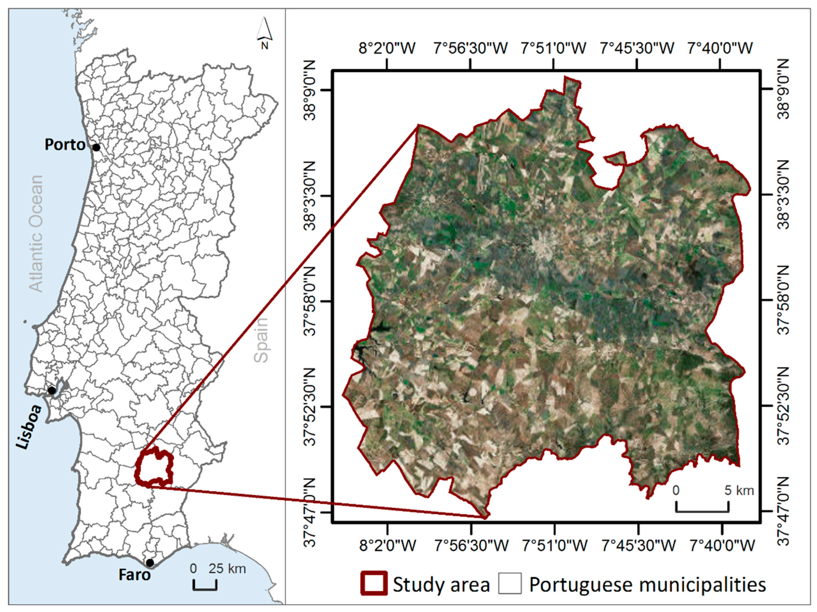
Figure 1. Study area (Basemap: true colour orthophotomap provided by ESRI/Digital Globe).
Remotesensing 11 01104 g001
Figure 2. Workflow for the long-term time series LULC methodology.
Remotesensing 11 01104 g002
Figure 3. Example of graphical display based on the discriminant factors (Df) values from the tclust cluster solution obtained with k = 2, α = 0.25 for one of the LULC classes. Larger Df values indicate not very “well-determined” clusters.
Remotesensing 11 01104 g003
Figure 4. Cluster process workflow.
Remotesensing 11 01104 g004
Figure 5. LULC classification maps for each period (1995–2015).
Remotesensing 11 01104 g005
Figure 6. LULC classification maps for 1995 and 2011.
Remotesensing 11 01104 g006
Figure 7. LULC classes (%) between 1995 and 2015.
Remotesensing 11 01104 g007
Table 1. Frequency by year of all available Landsat Level 2 data between 1995 and 2015 years.
YearNumber of ImagesYearNumber of Images
19951420068
19968200713
19971320088
199815200916
199912201012
200010201111
20011220120 *
2002520138
20036201414
200411201517
20058
* No available images.
Table 2. Normalized difference vegetation index (NDVI) and normalized difference water index (NDWI) equations.
Vegetation Index NameLandsat 4-5 ImagesLandsat 8 ImagesReference
NDVI B a n d   4   ( N I R ) B a n d   3 ( R e d ) B a n d   4   ( N I R ) + B a n d   3 ( R e d ) B a n d   5   ( N I R ) B a n d   4   ( R e d ) B a n d   5   ( N I R ) + B a n d   4   ( R e d ) [44]
NDWI B a n d   2   ( G r e e n ) B a n d   4 ( N I R ) B a n d   2   ( G r e e n ) + B a n d   4 ( N I R ) B a n d   3   ( G r e e n ) B a n d   5   ( N I R ) B a n d   3   ( G r e e n ) + B a n d   5   ( N I R ) [47]
Table 3. Descriptive statistics of the COS maps.
Nomenclature Level 1Nomenclature Level 2Class Coverage (1995)Class Coverage (2007)Class Coverage (2010)Class Coverage (2015)
1. Artificial surfaces1.1. Urban fabric1.4%1.5%1.6%1.6%
1.2. Industrial, commercial and transport units
1.3. Mine, dump and construction sites
1.4 Artificial, non-agricultural vegetated areas
2. Agricultural areas2.1 Temporary crops51.1%42.8%42.6%42.5%
2.2 Permanent crops5.7%9.1%11.9%13.1%
2.3 Pastures9.7%12.3%8.1%8.1%
2.4 Heterogeneous agricultural areas19.1%19.8%20.3%19.2%
3. Forest and semi natural areas3.1 Forests11.3%12.4%13.1%13.0%
3.2 Scrub and/or herbaceous vegetation associations
3.3 Open spaces with little or no vegetation
4. Wetlands4.1 Inland wetlands0%0%0%0%
4.2 Maritime wetlands
5. Water bodies5.1 Inland waters1.7%2.1%2.4%2.5%
5.2 Marine waters
Total100%100%100%100%
Table 4. Land use/land cover classes’ characteristics.
LULC ClassCOS Nomenclature CodeDescriptionImage ExampleField Example
Temporary crops with agroforestry areas2.1., 2.4.4Temporary crops (non-irrigated and permanently irrigated crops); complex cultivation patterns (herbaceous understory); land principally occupied by agriculture, with significant areas of natural vegetation; agroforestry areas. Remotesensing 11 01104 i001 Remotesensing 11 01104 i002
Permanent cropland2.2.Crops occupied the land for a long period and had a nonrotating regime (olive groves, vineyards) Remotesensing 11 01104 i003 Remotesensing 11 01104 i004
Permanent pastures2.3.Areas permanently occupied (≥5 years), with mainly herbaceous vegetation Remotesensing 11 01104 i005 Remotesensing 11 01104 i006
Forest3.1., 3.2., 3.3Areas occupied by tree clusters resulting from natural regeneration or planting Remotesensing 11 01104 i007 Remotesensing 11 01104 i008
Water5.1., 5.2.Freshwater surfaces, including watercourses and water plans (both natural and artificial) Remotesensing 11 01104 i009 Remotesensing 11 01104 i010
Table 5. Final number of samples per class.
LULC Class
Temporary Crops with Agroforestry AreasPermanent PasturesPermanent CroplandForestWater
Number of training samples19951158474684399648
20071062384474486456
2010786600630684402
2015828540636787588
Table 6. Error matrix of the map classification task (full period).
Reference Class
Map ClassTemporary Crops with Agroforestry AreasPermanent CroplandPermanent PasturesForestWaterTotalUser
Accuracy ± Error Tolerance
Temporary crops with agroforestry areas9343172614945301261674.06 ± 0.1%
Permanent cropland940133841080239055.98 ± 0.3%
Permanent pastures39510958870145066.07 ± 0.4%
Forest24192217510182396.42 ± 0.1%
Water00072055205599.66 ± 0.0%
Total10702309324781999206220334
Producer Accuracy ± Error tolerance87.30
± 0.1%
43.25
± 0.3%
38.66
± 0.3%
87.28
± 0.2%
100.0
± 0.0%
Overall Accuracy 75.96 ± 0.1%
Kappa index0.62