Article

Discrimination of Canopy Structural Types in the Sierra Nevada Mountains in Central California

1
Center for Spatial Technologies and Remote Sensing (CSTARS), University of California Davis, Davis, CA 95616, USA
2
The Climate Corporation, San Francisco, CA 94103, USA
3
Department of geology, geography and environment, University of Alcalá, Alcalá de Henares, 28801 Madrid, Spain
*
Author to whom correspondence should be addressed.
Remote Sens. 2019, 11(9), 1100; https://doi.org/10.3390/rs11091100
Submission received: 18 March 2019 / Revised: 21 April 2019 / Accepted: 6 May 2019 / Published: 8 May 2019
(This article belongs to the Special Issue State-of-the-Art Remote Sensing in North America 2019)

Abstract

:
Accurate information about ecosystem structure and biogeochemical properties is essential to providing better estimates ecosystem functioning. Airborne LiDAR (light detection and ranging) is the most accurate way to retrieve canopy structure. However, accurately obtaining both biogeochemical traits and structure parameters requires concurrent measurements from imaging spectrometers and LiDARs. Our main objective was to evaluate the use of imaging spectroscopy (IS) to provide vegetation structural information. We developed models to estimate structural variables (i.e., biomass, height, vegetation heterogeneity and clumping) using IS data with a random forests model from three forest ecosystems (i.e., an oak-pine low elevation savanna, a mixed conifer/broadleaf mid-elevation forest, and a high-elevation montane conifer forest) in the Sierra Nevada Mountains, California. We developed and tested general models to estimate the four structural variables with accuracies greater than 75%, for the structurally and ecologically different forest sites, demonstrating their applicability to a diverse range of forest ecosystems. The model R2 for each structural variable was least in the conifer/broadleaf forest than either the low elevation savanna or the montane conifer forest. We then used the structural variables we derived to discriminate site-specific, ecologically meaningful descriptions of canopy structural types (CST). Our CST results demonstrate how IS data can be used to create comprehensive and easily interpretable maps of forest structural types that capture their major structural features and trends across different vegetation types in the Sierra Nevada Mountains. The mixed conifer/broadleaf forest and montane conifer forest had the most complex structures, containing six and five CSTs respectively. The identification of CSTs within a site allowed us to better identify the main drivers of structural variability in each ecosystem. CSTs in open savanna were driven mainly by differences in vegetation cover; in the mid-elevation mixed forest, by the combination of biomass and canopy height; and in the montane conifer forest, by vegetation heterogeneity and clumping.

1. Introduction

Terrestrial ecosystems regulate the exchange of energy and matter between the land and the atmosphere [1]. Trees fundamentally define the three-dimensional structural and energetic properties of forest ecosystems including the amount of light energy intercepted for photosynthesis, which is subsequently available for respiration, and evapotranspiration [2,3]. Furthermore, the structural and biogeochemical traits within ecosystems may promote complementarity in energy use, including higher biomass and productivity that allow greater species coexistence in space, while vertically differentiated forest light strategies promote coexistence [4]. We lack information on the spatial and temporal variability of these physiological processes and the plant traits and geophysical parameters that drive exchanges in energy and matter. Jetz [5] identified the lack of this information as limiting our ability to understand global terrestrial ecosystem functioning and its influence on the Earth’s climate though the carbon, water, energy and nutrient cycles. Of particular concern is our inability to predict the status of carbon sequestration under future climates [6,7,8]. Better constraints on greenhouse gas (GHG) fluxes could be achieved with concurrently measured estimates of ecosystem functioning in terms of biogeochemical traits and three dimensional canopy structures. [9,10,11,12]. Measurement of horizontal and vertical canopy structure also provides quantitative information on wildlife habitat [13,14,15,16], and biodiversity [17].
To measure the spatial and temporal variability of physiological processes that drive exchanges of energy and matter between the land and the atmosphere, we need to map canopy biochemistry and structural properties, ideally measured simultaneously. Both LiDAR (light detection and ranging) and RaDAR (radio detection and ranging) have the capability to measure canopy structure [18,19], including height, biomass, and vertical structure. Although airborne LiDAR has limitations, it is widely accepted that it provides the best estimates of canopy structure, based on numerous studies over the past 20 years e.g., [18,20,21,22,23,24]. However, to obtain both biogeochemical traits and structure parameters requires measurements from both imaging spectroscopy (IS) and LiDARs. However, even when available, these data may not be acquired in the same season or even the same year, given cost and schedules. Combining archived LiDAR data with newly acquired IS data may limit the accuracy of retrieved spatial and temporal variability of the energy and mass exchange driving variables due to differences in weather conditions, growth stage, and disturbances of various types (defoliation, fertilization, irrigation, etc.) such that the structural variables no longer fit the biogeophysical variables.
We asked the question, is there another way to retrieve structure information? If so, can it be done concurrent with the IS acquisition? It is generally accepted dogma that vegetation structure is difficult or impossible to get with optical sensors alone [25]. Nonetheless, optical data have been used to estimate above-ground forest biomass from albedo or brightness e.g., [26,27,28]. Lu [26] developed models to estimate above-ground biomass with R2 close to 0.8 in a Brazilian Amazon successional forest and Zheng [27] estimated above-ground biomass with an accuracy of R2 0.67 using an independent validation dataset. Other studies have estimated forest structural properties from stereo imagery and LiDAR, with accuracies of R2 = 0.91 and R2 = 0.79 for height and biomass respectively [29], and combined optical and LiDAR data [30,31], with accuracies for tree high estimation of R2 = 0.84 and root mean square error (RMSE) = 7.3 m in the Sierra Nevada Mountains (California-USA) [30]. Huesca [32] estimated biomass, height and vegetation heterogeneity with accuracies higher than R2 = 0.8 for a mixed broadleaf and conifer forest in the Sierra Nevada Mountains (California, USA).
Because IS samples surface reflectance though many contiguous, narrow bands measuring the reflected solar spectrum between 400–2500 nm [33], the spectrum contains both absorbing and scattering bands, which provides information about both structure and process, thus the data has potential to capture important structural and physiological properties [34] that are not as well retrieved using broadband spectral data. For instance, IS has been demonstrated to map the distribution and concentration of many key canopy biochemicals and traits like leaf mass area (LMA), leaf area index (LAI), leaf water content (LWC) and leaf biomass [35,36,37,38,39,40,41,42,43,44]. This suggests that IS provides new opportunities to quantify ecosystem composition and function [9,10,11] and has promise for estimating the structural properties of forest canopies [31,32,45,46].
Most studies using IS data to map forest canopy structure have focused on a single site or forest type [47,48], or, have considered only a single structural variable, such as above ground biomass [31]. To truly capture the critical structural differences among forest types, forest canopy structure is better captured with a suite of metrics. Huesca [32] discriminated three canopy structural variables within a mixed conifer and broadleaf forest in the mid-elevation Sierra National Forest (California, U.S.A.), using the random forests model on a combination of spectral metrics sensitive to biomass, canopy height and spatial heterogeneity. This method allows simultaneous collection of both physiological and structural parameters, which are expected to lead to better estimates of gas exchange processes.
Machine learning methods such as random forests have become popular in remote-sensing studies and provide satisfactorily results in many ecological applications with remote sensing data [49,50,51,52]. This technique handles high volumes of data; it is fast and avoids overfitting. In addition, it provides a ranking of the most important metrics that then can be used to select the most relevant information, reducing data dimensionality [53].
The main objective of this research was to prove the usefulness of IS data to retrieve vegetation structure for forests with different species and structures in the central Sierra Nevada Mountains (California, U.S.A.). The specific objectives are (1) to develop generalized models to estimate structural variables (i.e., biomass, canopy height, vegetation heterogeneity, and forest clumping), using optical properties from IS metrics; and (2) to develop a methodology that use the structural variables to discriminate site-specific, ecologically meaningful descriptions of canopy structural types (CSTs). For example, pixels with low values of height, biomass, vegetation heterogeneity, and clumping represent sites with annual grasses or other low herbaceous cover species, while pixels associated with somewhat higher biomass and clumping typically represent shrublands or sparse tree cover if it is somewhat taller. In this research, LiDAR data was used as reference data to define the canopy structural variables and IS data was used to map these variables across the study area.
In Huesca [32] we assessed the relationship between optical metrics and structural variables derived from LiDAR. We used the IS-derived structural variables (canopy height, biomass, vertical distribution of foliage with height) to predict the CSTs, which allowed us to demonstrate that the combined metrics described different types of plant communities, from grasslands, to shrublands, to tall forests. This new paper advances the findings in [32] by identifying four structure variables compared to three, for sites covering a broader forested region of complex topography that represent three very different forested ecosystems: an oak-pine savanna, a mixed conifer/broadleaf mid-elevation forest, and a high elevation conifer forest. In Huesca [32] we defined CSTs with LiDAR data and then used Random Forests to define them with IS-derived structural metrics. In this paper we used the IS-derived and LiDAR-derived structural variables to define a procedure to that could be followed to identify CSTs in the three different ecosystems. Our hypothesis is that if we apply the same methodology to discriminate CSTs with LiDAR-derived and IS-derived structural variables and they both identify the same CSTs, then our methodology is consistent and robust.

2. Study Site, Materials and Methods

2.1. Study Site

Our study region is located on the western slopes of the Sierra Nevada Mountains of central California. We focus on three sub-regions (49.94 km2, 24.39 km2, and 134.02 km2) located coincidentally within the National Science Foundation (NSF) National Ecological Observatory Network (NEON) terrestrial sites in Domain 17 and which also overlaps with two sites and is near to the third site of the National Science Foundation’s Southern Sierra Critical Zone Observatory (CZO) (Figure 1). Our study areas are limited by the availability of LiDAR data acquired concurrently with IS data. The three sites represent forest types that are extensively distributed throughout the Sierra Nevada Mountains, in California.
The lower elevation site is located in the San Joaquin Experimental Range (abbreviated as SJER; located at 37°5′ N, 119°43′ W) and covers an elevation range from 210 m to 520 m above sea level. The area is characterized by open woodland savanna dominated by Quercus douglasii, Quercus wislizeni and Pinus sabiniana and generally associated with shrub species of Ceanothus sp., Arctostaphylos sp. and Aesculus californica, as well as various annual grass species. Summers in this Mediterranean climate are hot and dry with mean temperatures between 24 °C and 27 °C. Winters are cool and wet with mean temperatures ranging from 4 °C to 10 °C. The annual precipitation is around 486 mm, restricted to the extended winter period, from October/November to April/May [54], producing an annual drought duration of six or more months in the summer–autumn period.
The mid-elevation site is Soaproot Saddle (abbreviated as SOAP; located at 37°2′ N, 119°15′ W) in the Sierra National Forest and is situated approximately 998 m to 1383 m above sea level. The site is dominated by evergreen and deciduous broadleaf trees and mixed conifer forest. The main conifer tree species are Pinus ponderosa, Calocedrus decurrens, and Pinus lambertiana, and the most common broadleaf tree species are the deciduous Quercus kelloggii and the evergreen Quercus chrysolepsis. Forest density varies from dense to relatively open. Summers are hot and dry, and winters are mild and wet. The mean temperature varies from 5.5 °C to 18.0 °C, and the annual precipitation is around 805 mm per year [55].
The highest elevation site is the Teakettle Experimental Forest (abbreviated as TEAK; 36°58′ N, 119°1′ W) located within the Sierra National Forest at elevations from 2000 m to 2800 m above sea level and mainly characterized by montane old-growth conifer forest dominated by Abies concolor, Abies magnifica and Pinus jeffreyi. Forest mosaics range from patches of dense canopy, scattered trees, or shrub-dominated together with open rocky areas. Summers are cooler than lower elevations but are also dry and winters are cool and moist, with snow typically covering the ground from November to June. Most of the 1250 mm annual precipitation falls as snow between November and May [56].

2.2. Data and Methods

Figure 2 shows the methodology flowchart. Two remotely-sensed datasets were used in this research: (1) Small footprint, discrete return-recording LiDAR (Optec Gemni) from the NSF NEON program and (2) IS data from the National Aeronautics and Space Administration’s (NASA) Advanced Visible Infrared Imaging Spectrometer (AVIRIS-classic). The former was used to produce the reference structural data, while the latter was trained to predict the structural variables measured by LiDAR. In addition, LiDAR metrics were used to validate the IS models due to the accuracy of the LiDAR data and the lack of field data for the four predicted structural variables. Previous studies have used LiDAR as reference data for validation [57]. We evaluated the accuracy of the LiDAR canopy height prediction by comparing it to studies in the literature [18,58,59,60,61,62,63,64,65,66,67], which reported coefficients of determination (R2), between 0.70 and 0.95 [61,62,63,64,65,66,67] in ecosystems similar to our study sites [67]. Several studies estimated conifers, like those present in our study sites, with height errors less than two meters [61,66,68,69,70] in sites with species from mixed and broadleaf forests with different vegetation densities and tree species compositions [71,72]. To evaluate our LiDAR height data directly, we compared maximum heights of LiDAR with field observations (see Supplementary Materials Figure S1) obtaining an agreement of R2 = 0.80 and a RMSE of 2.38 m which validates the use of the LiDAR data as reference data for this analysis.
The research took place in two phases (Figure 2). In the first phase, four structural variables were selected from LiDAR. We built general, non-site-specific models to estimate the four structural variables (i.e., biomass, canopy height, vegetation heterogeneity, and clumping) using optical metrics from AVIRIS-classic and using LiDAR data as reference data to train, test and validate the model. In the second phase, combinations of the structural variables were used to define spatially explicit site-dependent CSTs. The procedure was carried out in parallel using IS-estimated structural variables and LiDAR-derived structural variables. In a final step CST results from IS-derived data and LiDAR-derived data were compared to validate the procedure.

2.2.1. Advanced Visible Infrared Imaging Spectrometer (AVIRIS) and Light Detection and Ranging (LiDAR) Preprocessing

AVIRIS-classic data were acquired June 12, 2013 by the Jet Propulsion Laboratory (JPL). The sensor was flown onboard an ER-2 aircraft at approximately 20 km altitude, resulting in a pixel spatial resolution of 18 m. AVIRIS-classic has 224 spectral bands ranging from 370 nm to 2500 nm with a nominal bandwidth of 10 nm [73]. JPL provided radiometric, geometric and atmospheric correction to apparent surface reflectance. In addition, a topographic correction was done following the model proposed by Soenen [74] based on the sun-canopy-sensor (SCS) correction proposed by Gu and Gillespie [75]. The noisy atmospheric water bands from 1342 nm to 1482 nm and from 1800 nm to 1966 nm were removed, leaving 193 bands for the analysis.
Small footprint, discrete return-recording Optec Gemni LiDAR data from the NEON Airborne Observation Platform (AOP) were collected for the three study sites on 9–15 June 2013 coincident with the NASA IS data [76]. The areas covered by the LiDAR acquisition are shown in the red boxes in Figure 1. The data have a point density of ~19 pts/m2. In addition, a 1 m2 spatial resolution bare earth digital elevation model (DEM) was created by NEON, which was used to normalize the height returns. All LiDAR-derived structural metrics were calculated on an 18 m grid that was co-registered with AVIRIS-classic data pixel using 100 ground control points with an RMSE of < 0.5 pixel. We removed pixels without green vegetation using a two-step masking process: (1) pixels with Normalized Difference Vegetation Index (NDVI) <0.2 and of these, (2) pixels that were considered non-photosynthetic vegetation (non-green plant material) when un-mixed using multiple endmember spectral mixture analysis (MESMA) [77]. The low NDVI threshold selected was based on the decision to use a common criterion valid for all three study sites. This was especially important at the SJER site due to low canopy cover in the savanna ecosystem, together with the summer timing of the data acquisition (i.e., when the understory is dominated by dry grass). These steps resulted in masking rock outcrops and water bodies in the images but did not remove all the roads as pixels were partly vegetation covered.

2.2.2. Optical and LiDAR Metrics

The optical metrics were based on Huesca [32]:
(1).
Sub-pixel cover fractions of Green Vegetation (representing different forest cover types), Soil, Non-Photosynthetic vegetation (NPV), and shade were calculated using MESMA implemented in the Visualization and Image Processing for Environmental Research (VIPER) Tools package using ENVI image analysis software [78]. MESMA was run with the following constraints: 1. the maximum allowable RMSE = 2.5% and 2. the minimum and maximum allowable endmember fractions must fall between −0.05 and 1.05. Spectra of NPV and soil endmembers were independently collected during the overflight using an Analytical Spectral Devices (ASD) full-range spectrometer sensor, the FieldSpec3 Spectroradiometer (Analytical Spectral Devices Inc., Boulder, CO, USA), while green vegetation endmembers were selected from the AVIRIS-classic images. Several endmember spectra were selected for each cover type. The final endmembers chosen had high COB (count-based endmember selection (COB: [79])) and low MASA (minimum average spectral angle (MASA: [80])) and EAR (endmember average RMSE (EAR: [81])) values.
(2).
Narrow-band indices representing three types of spectral information were used: 1. those sensitive to the presence of photosynthetic pigments: NDVI [82], Red Edge Normalized Difference Vegetation Index (NDVI705) [83,84], Modified Red Edge Normalized Difference Vegetation Index (mNDVI705) [84,85], and Enhanced Vegetation Index (EVI) [86]; 2. those sensitive to water content: Normalized Difference Water Index (NDWI) [87], Normalized Difference Infrared Index (NDII) [88], and 3. an index sensitive to dry plant matter content: the Cellulose Absorption Index (CAI) [89]. Despite the similarity of these indexes, they provide different projections through the data space related to these processes and each provides useful information, as described later in the Results section. The formulas of the narrow-band indices used in this research are shown in Supplementary Material Table S1.
(3).
Spectral canopy water absorption derivatives: Derivative analysis was used to measure the wavelength position and magnitude of the NIR water absorption edges [90], abbreviated here as Wtr1EdgeWvl and Wtr1EdgeMag, the canopy water absorption features between 958–1073 nm and 1105–1168 nm, abbreviated as Wtr1AbAr and Wtr2AbAr, respectively, and the physically-derived equivalent water thickness (EWT; the depth of water/per pixel area) [90,91,92].
(4).
Principal component analysis (PCA) [93] was performed both using the full spectral range, as well as the independent regions: visible, near infrared, and shortwave infrared which was done to summarize significant information in all three regions of the spectrum. The PCA components that provided strong relationships with canopy structure [32] were included in this study.
The LiDAR metrics selected were those in Huesca [32], including maximum height (Hmax), mean height (Hmean), median height (Hmedian) and standard deviation of canopy height (Hstd), which were derived from the height distribution of the LiDAR returns. To avoid outliers, the 99th percentile was used to assign the maximum height. The standard deviation of the canopy height model (CHMstd) was created at 1 m2 spatial resolution. The fractional cover (FC) [21,94] and the fractional cover from the first returns (FC_1ret) [21] represent the vertical projection of the vegetation canopy onto the ground calculated as the ratio between vegetation and ground returns. FC is based on all returns while FC_1ret only considers the first returns. Leaf area index (LAI) [95] is estimated from the canopy cover. The integral of the vegetation vertical profile (VVPint) at 0.5 m vertical resolution, represents the proportion of canopy returns for each height bin and is used to estimate biomass [96,97]. In addition, we computed the clumping index using the method of García [23] to estimate the degree of randomness of the spatial distribution of canopy materials. The term clumping/randomness refers to the spatial distribution of the vegetation within our 18 m pixels. Although usually applied to the degree of randomness of leaves/needles or shoots, it is not restricted to a specific scale but can be applied to the degree of clumpiness or randomness of the crowns or in the case here, the vegetation within the pixel. The clumping index was not included in Huesca [32] due to distortion in some of the flight lines. This problem was fixed by the NEON team, and used in this analysis [76].

2.2.3. LiDAR-Derived Structural Variables

The relationship among all 10 LiDAR metrics was measured by Pearson’s R coefficient (R) (Supplementary Materials Table S2). Results showed strong inter-correlations among LiDAR metrics in the three study sites, ranging from −0.7 to 1.00. Thus, we grouped the highly correlated metrics into variables related to biomass (composed of VVPint, LAI, FC, and FC_1ret, with cross-correlations between 0.91–1.0), variables related to canopy height (composed of Hmean, Hmedian and Hmax, with cross-correlations between 0.79–1.0), variables related to vegetation heterogeneity or canopy roughness (composed of Hstd and CHMstd, with cross-correlations between 0.96–1.00), and the clumping index, which had the least correlation to the other structural variables and was treated as an independent variable.
In this study, the metrics selected from the mid-elevation site, were chosen to represent each metrics group and were based on the variable that presented the highest correlations. The metric Biomass was most strongly represented by the vertical distribution of canopy elements (VVPint). Hmean represented canopy height, and CHMstd represented vegetation heterogeneity. CHMstd is a continuous metric that represented vegetation heterogeneity based on canopy heights. The clumping index represented how the vegetation is distributed in the space; that means the degree of clumpiness or randomness of the vegetation. Both structural variables (i.e., CHMstd and clumping index) represent horizontal structural variables. Of the four selected structural variables, biomass and height can be considered “vertical vegetation variables”, and vegetation heterogeneity and clumping can be considered “horizontal vegetation variables”.

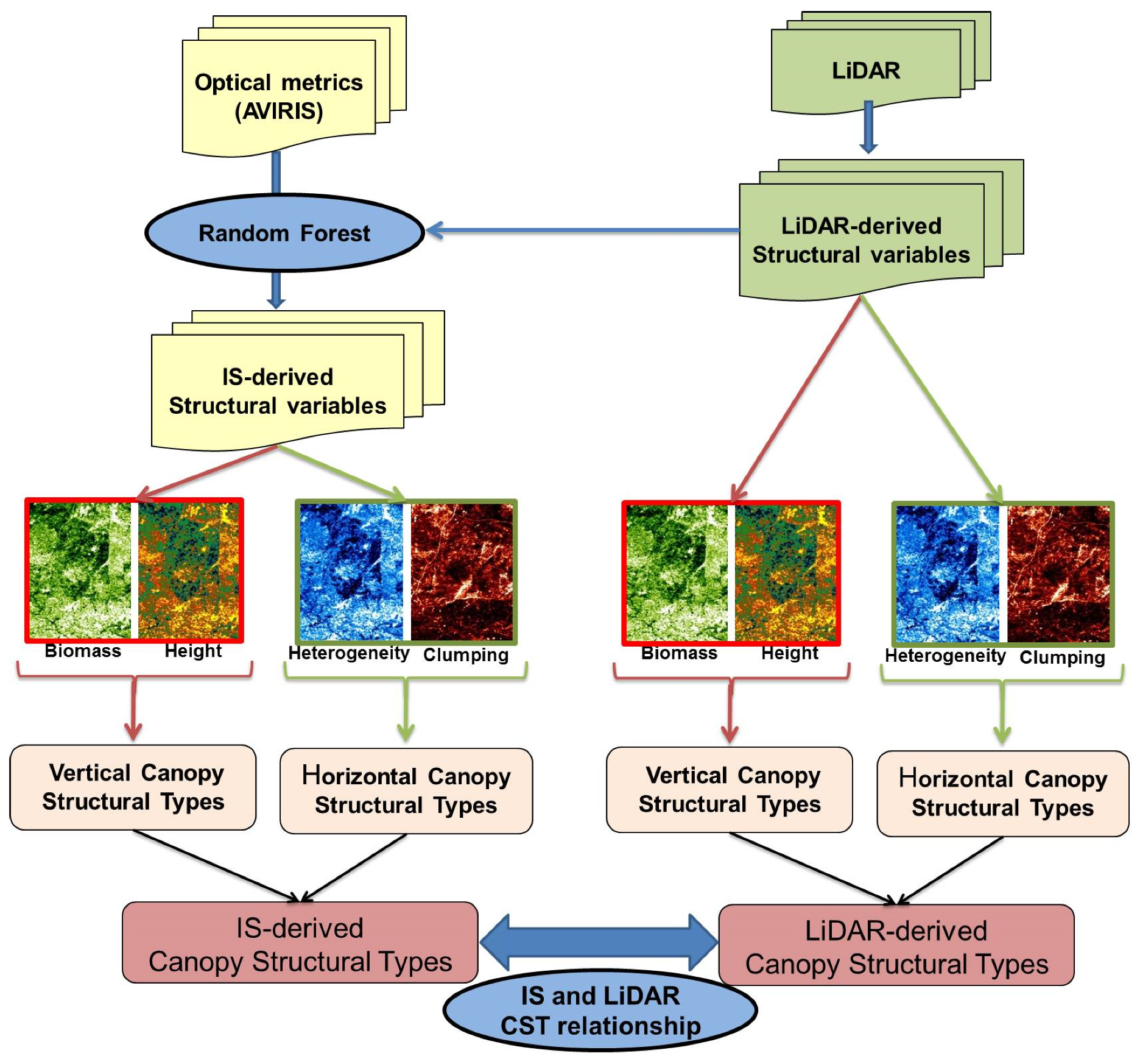
2.2.4. Modeling Structural Variables with Optical Metrics

We developed a single, cross-site model for each of the final four structural variables (i.e. biomass, vegetation height, vegetation heterogeneity and clumping), estimating them with the optical metrics defined in Section 2.2.2 using the random forests model. It is a non-parametric non-linear tree-based regression model [98]. The number of decision trees was initially selected by running the procedure 1000 times and analyzing the regression error. At 200 trees, the error stabilized and, to set a conservative limit, we chose 500 iterative trees to ensure that every observation was predicted multiple times. The random forests model randomly selects the best fit four optical metrics from the 24 possible metrics (Table 1). These combinations can be different in each tree; therefore, over the 500 runs the relative strength of each metric on model performance was established.
In order to evaluate the reliability of each model, one set of data was used to develop the model (i.e., training-testing dataset), and another independent dataset was used to evaluate the model’s reliability (i.e., validation dataset). Training and validation were selected to be sufficiently far apart to avoid any spatial autocorrelation. The Moran I correlogram was used to estimate the minimum distance apart validation points needed to be from training points to avoid spatial autocorrelation. At each iteration, the training step used 1/3 of the independent testing-training data and the remaining 2/3 was used for internal testing of the model. The training-testing dataset was selected from North to South over the western part of each site, and the validation dataset from North to South over the Eastern part with a separation of 2.5 km, 1.0 km, and 1.4 km for SJER, SOAP and TEAK, respectively, in order to capture the maximum variability of each structural variable while avoiding the spatial autocorrelation.
The complex terrain and difficult access to areas with steep slopes, compounded with large gradients and clustered species distribution patterns made it difficult to find an unbiased sampling plan for these training, testing, and validation datasets. We employed a dual-validation method to evaluate (1) the R2 and (2) the spatial extendibility of the models. Each model’s accuracy and precision was evaluated by its R2 and the model’s error using the RMSE and the mean percent standard error (MPSE). Sometimes RMSE can be difficult to interpret because it depends of the range of the variable, therefore, we also report the ranges of each variable among other basic statistics (Supplementary Materials Table S3). (2) The spatial extendibility of the model was evaluated over an independent validation data for each study site by assessing the relationships measured by R2, and RMSE between the AVIRIS-classic estimated structural variables values and the LiDAR data. By spatial extendibility we mean that a statistical model developed from the training-testing data was compared to an independent validation dataset, which was obtained from the image at locations sufficiently separated beyond the distance determined by the spatial autocorrelation test at each site, but within its elevation zone community type. This validation evaluates the robustness of the model at each site. We also tested for spatial autocorrelation of the errors for each structural variable in each study site using Moran’s I index. We present the ranking of the most important metrics based on the increase in the random forests’ mean square error if they were deleted from the composite structural variables.

2.2.5. Canopy Structural Types Definition

We wished to understand how these four structural variables (i.e., biomass, vegetation height, vegetation heterogeneity and clumping) related to different forest types in the three study sites. While the generic model was developed to produce the four structural variables using data from all three study sites, we used these to develop a set of CSTs that were defined site by site. Our objective here is to develop a procedure to identify CSTs. This procedure was applied independently to both LiDAR-derived structural variables (i.e., those used as reference data) and to the IS-derived structural variables (i.e., used as predicted structural variables). We then compared the CSTs derived from these two data sources. In addition we wanted to evaluate how CSTs varied within and between sites that are characterized by differences in climate, topography, soils, community composition, community types, and frequency of disturbance.
CSTs are defined by the combination of vertical and horizontal structure variables. Vertical structure is represented by biomass and height while horizontal structure is represented by vegetation heterogeneity and clumping. In a first step each variable was to be divided into several classes. The number of classes is defined by the user and depends on the requirements of a specific research objective. For this study we classified biomass and height into three classes that represented low, medium and high values. Vegetation heterogeneity was classified into two classes that represents homogeneous (i.e., low values) and heterogeneous (i.e., high values) pixels. Clumping was also classified into two classes that represented clumping distribution of trees (i.e., low values) s versus random distribution of trees (i.e., high values).
An unsupervised IsoData classification [99] was used to classify biomass, height and vegetation heterogeneity. This procedure calculates evenly distributed class means within the dataset, and then iteratively clusters the pixels into the nearest class. However, the clumping was classified using a static threshold of 0.5, with values above 0.5 indicating regular to random distribution, and values below 0.5 indicating clumped aggregation (where 0 = completely clumped, 1 = completely random; Garcia et al., 2015).
The combination of biomass and height classifications created a maximum of 9 vertical structure classes (3 biomass classes combined with 3 height classes). Each class was analyzed in terms of representativeness (i.e., number of pixels and spatial continuity) and the proximity among classes with the intent to reduce the number of combinations to an interpretable and ecologically meaningful set. The final selection of classes represents what we called “vertical canopy structural types” (VCSTs). The combination of vegetation heterogeneity and clumping resulted in a maximum of 4 horizontal structure classes (2 vegetation heterogeneity classes combined with 2 clumping classes). Each class was analyzed following the same criteria explained above. The final selection represents what we called “horizontal canopy structural types” (HCSTs). In a final step, VCSTs and HCSTs were combined. Each class was analyzed in terms of representativeness (i.e., number of pixels and spatial continuity) and the proximity among classes to define the final CSTs.
One class is selected as potential VCST, HCST, or as the final CST when it represents more than 15% of the pixels of the study site and shows spatial continuity (or coherence). Those representing less than 15% were merged with one of the previous classes based on the average class proximity and spatial coherence. One additional rule in the merging process was that a high class value for any structural variable cannot be combined with a low class value. This restriction means that a high biomass pixel cannot be joined with a low biomass pixel or high height with low height. The other classes that could not be grouped and represent less than 15% of the pixels of the study site were evaluated as to whether they should be grouped together or considered as a different class.
The next step was to ecologically interpret the CSTs for each study site using the U.S. Forest Service’s vegetation map of California (CALVEG), updated in 2015 [100]. It provides information on vegetation cover types and attributes, such as crown size and height. CALVEG is the best source of spatial information about these sites, and produced at the same spatial scale and for the same time period, and CVEG provided independent information on the ecological status of these forests. Two attributes within CALVEG were used to conduct this analysis: (1) Vegetation Cover Type and (2) National Vegetation Classification Standard (NVCS). Within the latter, only the classes of “closed tree canopy” and “open tree canopy” were considered. Each CST is described with the percentage of each class attribute. The sum of all “vegetation cover type” classes within in each CST sums to 100%, however the sum of the two selected classes from the NVCS classification are not required to equal 100% because they do not represent all classes within this attribute. Table 2 presents the classes defined within the vegetation cover type attribute.

3. Results

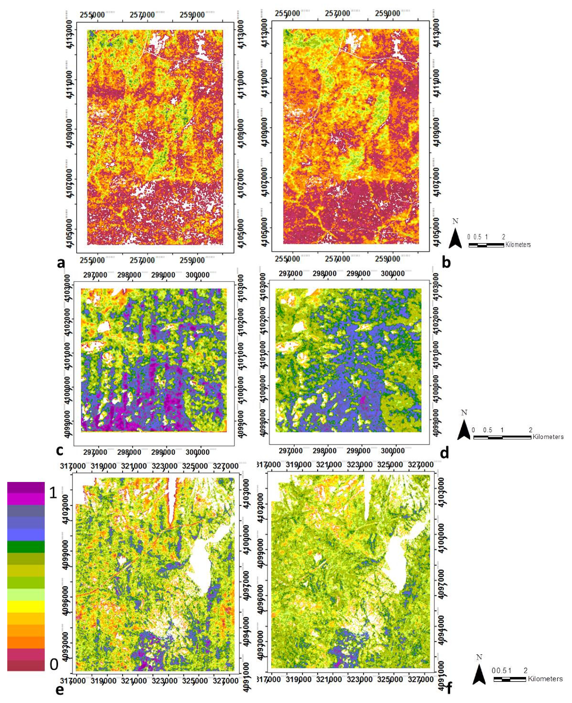
3.1. Modeling Structural Variables with Optical Metrics

Random forest regression models for all four structural variables achieved high goodness-of-fit, with R2 values of 0.83, 0.80, 0.78 and 0.76, and RMSEs of 0.01, 1.08, 2.82, 0.01 for biomass, canopy height, vegetation heterogeneity, and clumping, respectively (Table 3, Figure 3, Figure 4, Figure 5 and Figure 6). Clearly the spatial patterns for the structural variables between LiDAR and optical data closely match for all four variables at all three sites, even with the banding observed in the clumping images (Figure 6). Additional information about the correlations between the LIDAR variables and structural variables at each study site are provided in the Supplementary Materials Figure S2. The relationship between the four structural variables and the most important optical metrics are shown in the Supplementary Materials Table S4.
To evaluate the site-specific performance of the general models, we see they produced IS-derived maps that were similar to LiDAR-derived maps at each site, although some differences are observed (Table 3). By examining the R2 correlations within the training-testing and validation datasets compared to the reference data (i.e., LiDAR-derived structural variables) for each of the four structural variables, R2 values were greater than 0.70 for the training dataset for all variables except height in SJER and TEAK, and equal or above 0.58 in SOAP. Lowest accuracies were found using the validation dataset for each study site, which was especially evident in SOAP, but nontheless with low RMSE. However, considering the independent validation data for the three study sites together, the R2 values were 081, 0.69, 0.72 and 0.70 for biomass, canopy height, vegetation heterogeneity and clumping respectively. Biomass was the structural variable with highest R2 at all study sites (i.e., R2 of 0.80, 0.66 and 0.8 in SJER, SOAP and TEAK respectively) and height was the structural variable with lower R2 in SJER and SOAP (i.e., R2 of 0.67 and 0.59, respectively) and clumping in TEAK (R2 of 0.72).
SJER (Figure 3a,b, Figure 4a,b, Figure 5a,b and Figure 6a,b) and TEAK (Figure 3e,f, Figure 4e,f, Figure 5e,f and Figure 6e,f) show similar overall fit for biomass, vegetation heterogeneity and clumping for the training dataset with R2 equal or greater than 0.72. But in general terms TEAK presents lower R2 for three of the four variables (except biomass) in the validation dataset. TEAK has higher R2 for height compared to SJER for both training and validation datasets with R2 of 0.78 and 0.57 for training and validation respectively versus 0.67 and 0.40 for training and validation respectively in SJER. SOAP had the lowest R2 values for the four structural variables (Figure 3c,d, Figure 4c,d, Figure 5c,d and Figure 6c,d), but they are still within the range of other classifiers with R2 values of 0.66, 0.59, 0.64 and 0.58 for biomass, canopy height, vegetation heterogeneity and clumping respectively using the training dataset. Much lower values are found in SOAP for the validation data with R2 values of 0.35, 0.33, 0.52 and 0.17 for biomass, canopy height, vegetation heterogeneity and clumping respectively. This site has the most complex vegetation in terms of species number and types, but it is the smallest area by 2–5 times the other two sites, providing a potential explanation for its lower performance.
Examining the spatial distribution of model errors at each site, we found no coherent spatial pattern for errors in SJER (Supplementary Materials, Figure S3a–d) except for clumping. This was also true for canopy height and heterogeneity at SOAP (Supplementary Materials, Figure S3f,g). The highest errors for biomass and clumping (Supplementary Materials, Figure S3e,h) were concentrated in the southwest part of the SOAP study site, where the model underestimates the values. At TEAK (Supplementary Materials, Figure S3i–l), we observed clear spatial patterning in model errors for all variables except clumping (S3l). Strong striping was observed for clumping at all sites (Supplementary Materials, Figure S3d,h,l). Moran’s I index showed significant positive spatial autocorrelation that is in agreement with the spatial patterns observed. The highest errors in biomass were found in the southwest and northwest parts of the TEAK study area, the highest errors in canopy height were also in a southwest to northeast band, and the highest errors in vegetation heterogeneity were in the southwest (Supplementary Materials, Figure S3j,k), respectively. Those areas correspond to extreme values of the variable (i.e., either very high or very low), at least partially due to the regression approach used for estimating these structural variables.

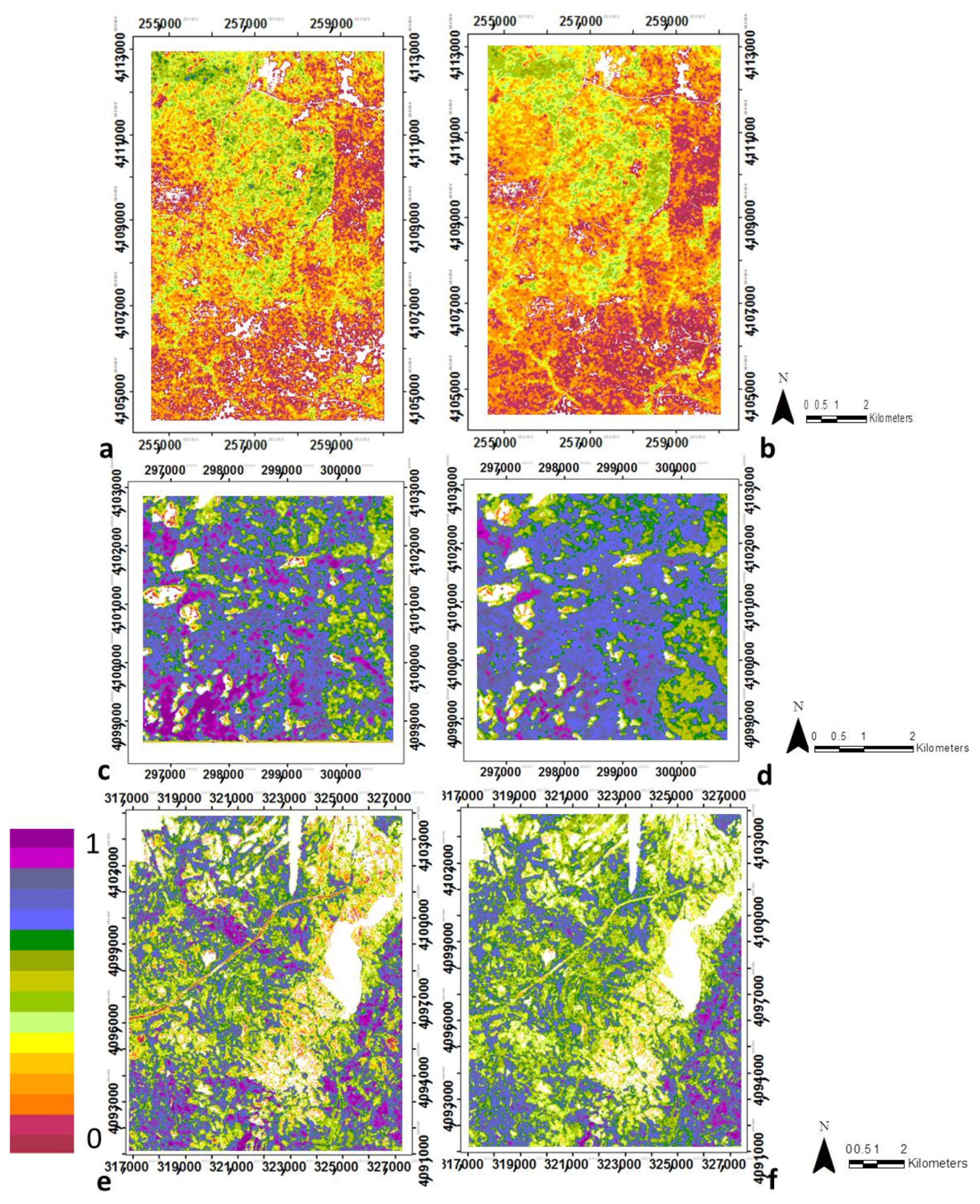
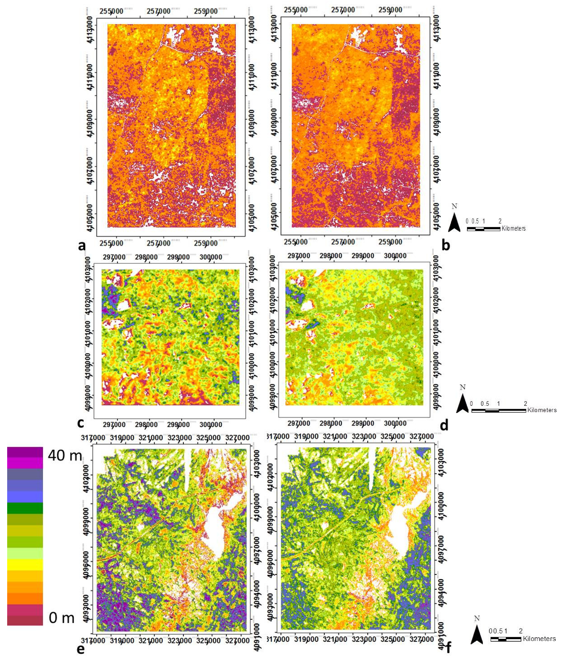
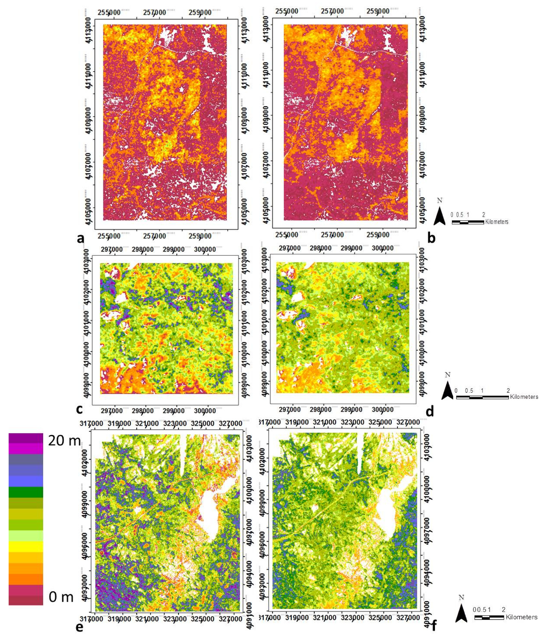
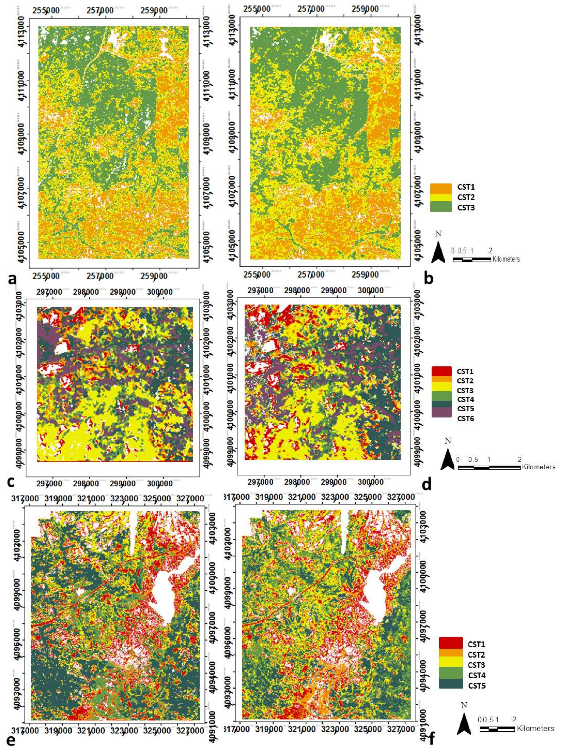
3.2. Canopy Structural Types (CSTs)

Result from the analysis of CSTs is shown in Figure 7 and Table 4. Each CST represents different patterns of biomass, height, vegetation heterogeneity and clumping within the forest (Supplementary Materials Figure S4). The coherent spatial distribution of each CST show the class may consistently represent a forest type or condition. Table 5 shows the percentage of each vegetation cover type from CALVEG within each CST. Only the results from the IS-derived data are displayed in Table 5 for SJER and SOAP because the differences between LiDAR-derived and IS-derived data were negligible. For TEAK, both are displayed (i.e., LiDAR-derived and IS-derived data) because there is a disagreement in one of the CST classes. Supplementary Materials Figure S5 presents a red–green–blue (RGB) combination, equivalent to the fractional composition of each of the three most important structural variables at each site. We present this figure to demonstrate that the number of CSTs identified in our analysis (Figure 7) is consistent with the patterns seen in Supplementary Materials Figure S5 and these results are spatially coherent. Supplementary Materials Tables S6 and S7 show the agreement between CSTs derived from LiDAR and IS data.

3.2.1. Structural Types Defined in the San Joaquin Experimental Forest

Of the nine potential classes from the combinations of biomass and canopy height (i.e., vertical structure), we found three different vertical canopy structural types (VCSTs) at SJER, representing low biomass and low height, medium biomass and medium height, and high biomass and tall height. Within the four possible classes from the combinations of vegetation heterogeneity and clumping (i.e., horizontal structure), there were just two horizontal canopy structural types (HCSTs) discriminated because most pixels were classified within the low clumping class. Thus, differences between these two combined classes are based on mainly on vegetation heterogeneity. Finally, the six classes from combing the VCSTs and HCSTs were grouped into three unique CSTs (Figure 7a,b and Table 4).
Differences among CSTs at SJER were driven mainly by vertical structure. In general terms, low to medium biomass (i.e., mean biomass between 0.06 and 0.18) and canopy height (i.e., mean canopy height between 1.86 and 4.28 m) were associated with more homogeneous areas (i.e., mean vegetation heterogeneity between 0.62 and 1.49), while high biomass and tall canopy height (i.e., mean biomass and canopy height higher than 0.30 and 6 m respectively) characterized more heterogeneous areas (i.e., mean vegetation heterogeneity greater than 2.5). Following the procedure described in the methods section, the CSTs were independently determined using LiDAR-derived structural variables and IS-estimated structural variables (Figure 7a,b).
Table 5 shows the percentage of each vegetation cover type from CALVEG within each CST. Only the results from the IS-derived data are displayed in Table 5 because the differences between LiDAR-derived and IS-derived data were negligible (see Table 4). The first CST is dominated by grass species (74%). The second CST is dominated by a mix of hardwood species and grass (43% hardwood and 53% grass). The third canopy structural type is mainly dominated by hardwood species (55% hardwood, 27% hardwood/conifer mixed).

3.2.2. Canopy Structural Types Defined in Soaproot Saddle

At SOAP, analysis of the nine possible classes from vertical structure (i.e., the combinations of biomass and canopy height) resulted in five VCSTs. The four classes resulting from the horizontal structure (i.e., the combinations of vegetation heterogeneity and clumping) were sufficiently representative and distinct that they were not grouped. The 20 final classes from the combinations of VCSTs and HCSTs were grouped into six different CSTs (Figure 7c,d and Table 4).
The similarity between CSTs obtained from LiDAR-derived variables and from IS-derived variables is clear (Figure 7). CST1 and CST6 are characterized by low and high values of structural variables, respectively. The other four CSTs represent intermediate situations. CST4 and CST5 represent medium biomass (i.e., mean biomass between 0.57 and 0.70) and high vegetation heterogeneity (i.e., mean vegetation heterogeneity between 7.61 and 8.93) together with a regular to random distribution of the vegetation (i.e., mean clumping between 0.44 and 0.65). The difference between these CSTs is in canopy height. While CST4 is characterized by medium canopy height (i.e., mean height around 12–14 m), CST5 is dominated by taller canopies (i.e., mean height around 15–16 m). There is a difference in terms of biomass between CST2 and CST3 from LiDAR-derived and IS-derived data. CST2 and CST3 are represented by medium and high biomass respectively with LiDAR-derived data but by low and medium biomass respectively with IS-derived data. Both CSTs are characterized by homogeneous vegetation, however, while CST2 is associated with medium canopy height and clustered vegetation aggregations (i.e., mean canopy height around 11–12 m and mean clumping around 0.4), CST3 is characterized by low canopy height and by regular to random distribution of the vegetation (i.e., mean canopy height around 8–9 m and mean clumping around 0.59–0.70).
Table 5 shows the range in percentage for each CST of each CALVEG vegetation cover type together with the attributes of closed and sparse tree canopy from the national vegetation classification standards. Only the results from the IS-derived data for TEAK are shown in Table 5 because the differences between LiDAR-derived and IS-derived data for JSER and SOAP were negligible (See Table 4). All CSTs are dominated by mixed forest (Table 5) according to CALVEG data with an increasing percentage from CST1 to structural type CST6 (from 49% in CST1 to 73% in CST6). Hardwood species dominate the first three CSTs while conifer species dominate the last three CSTs. The first CST is associated with low values of the four structural variables and has a relatively high percentage of sparse tree canopy and non-vegetated areas (i.e., 29% and 17% respectively) in relation to the other CSTs. The main difference between CST2 and CST3 is based on the vegetation distribution (i.e., clumping) (Table 5). According to CALVEG, CST3 has a higher percentage of hardwood forest, and it is mainly associated with more closed forests than CST2, which has a high percentage of open forest that is associated with a clumped distribution. The differences between CST4 and CST5 are in canopy height and clumping, which is medium and high, respectively, for CST4, and high and low, respectively, for CST5. These results can be explained in terms of vegetation distribution. Although CST5 has a higher percentage of coniferous forest, it is more open than CST4, thus the former presents a greater degree of clumping as represented by lower values of the clumping index. CST6 is characterized by high values of all structural variables; this is in agreement with the CALVEG classes because these pixels are mainly associated with high percentage of conifer forest (26%) with a closed tree canopy (90%).

3.2.3. Structural Types Defined in Teakettle Experimental Forest

At TEAK, analysis of the nine possible classes from the vertical structure resulted in three different VCSTs that represent low, medium and high biomass and height. The four HCSTs resulting from the horizontal structure were again sufficiently different to be representative and distinct, therefore they were not grouped. Finally the 12 resulting classes from the combination of VCSTs and HCSTs were grouped into five different CSTs (Figure 7e,f and Table 4).
CST1 is characterized by low values of the four structural variables. CST2 and CST3 are characterized by medium biomass but the rest of the structural variables are different. While CST2 represents small, homogeneous and regular to random distribution of vegetation (i.e., mean canopy height between 5-8 m, mean vegetation heterogeneity between 3.93 and 5.12 and mean clumping higher than 0.5), CST3 is characterized by tall, heterogeneous canopies in terms of tree heights and clustered aggregations of forest trees (i.e., mean height taller than 14 m, mean vegetation heterogeneity greater than 7.0 and mean clumping less than 0.5). In this site, there was disagreement between CST4 and CST5 in terms of clumping. CST4 represents random distribution in LiDAR-derived data but a clumping distribution in IS-derived data and the opposite situation occurs in CST5.
Table 5 shows the percentage of each CALVEG vegetation cover type within each CST together with the attributes of closed and sparse tree canopy from the national vegetation classification standards. At this site, the differences between LiDAR-derived data and IS-derived variables were not negligible in one of the CSTs, thus Table 5 provides both results. TEAK is mainly dominated by coniferous forests but the percent of that dominance is different among structural types. CST1, has low values of the four structural variables, and is associated with a higher percent of sparse low stature vegetation (28% and 32% for LiDAR-derived and IS-derived data, respectively) and non-vegetated area (17% and 18% for LiDAR-derived and IS-derived data, respectively). CST2 had higher structural variables than CST1 (i.e., medium biomass, low canopy height and vegetation heterogeneity, and high clumping) that is associated with the highest percentage of mixed forest (13% and 20% for LiDAR-derived and IS-derived data, respectively) and the lowest percentage conifer forest (55% and 51% for LiDAR-derived and IS-derived data, respectively). Pixels within CST3, CST4 and, CST5 are more than 70% conifer forest. CST3 is associated with more open and sparse tree canopy (16% and 15% for LiDAR-derived and IS-derived data, respectively) than CST4 and CST5. This explains the lower values of biomass and canopy height in CST3. The main difference between CST4 and CST5 is the clumping. Both CSTs are dominated by high percentage of coniferous forest, but CST5 has a greater closed tree canopy percentage (70% and 84% for LiDAR-derived and IS-derived data, respectively) than CST4 (59% and 58% for LiDAR-derived and IS-derived data, respectively). The main disagreement between LiDAR-derived and IS-derived data is the proportion of mixed and conifer forests between CST4 and CST5. While the percentage of conifer and mixed forest is similar for both CSTs using IS-derived data (97% and 93% of conifer for CST4 and CST5 respectively, and 1% and 6% of mixed forest for CST4 and CST5 respectively), the conifer percentage is much higher and mixed forest percentage is much lower for CST5 than CST4 using LiDAR-derived data (77% and 94% of conifer for CST4 and CST5, respectively, and 14% and 5% of mixed forest for CST4 and CST5, respectively).

4. Discussion

Our results demonstrate how IS data can be used to create comprehensive and easily interpretable maps of canopy structural types across the major forest ecosystems of the Sierra Nevada Mountains, California. The models developed provide accurate estimates of four structural variables (i.e., biomass, canopy height, vegetation heterogeneity and clumping) across three study sites, demonstrating their applicability to a diverse range of ecological types from an open savanna, to a dense conifer/broadleaf mixed forest to a clumped distribution of trees in a high elevation montane conifer forest, using a single, general model for each variable. We illustrated the spatial extendibility of each model using an independent validation dataset that was tested (1) to show it had low spatial autocorrelation, and (2) that it was not used in the training phase for model development.
We developed and tested a general model to estimate structural variables using IS data for three structurally and ecologically different forested sites in the central Sierra Nevada Mts. Our study provides a methodology to discriminate ecologically meaningful “canopy structural types” (CSTs) that further refined and tested the approach of Huesca [32] to map forest structural variability based on “canopy structural types” derived from IS data. The CSTs are site-specific and capture the major structural differences and trends within each ecosystem. The number of CSTs provides information about the canopy complexity of the ecosystems. Accurate maps of forest canopy structures are critical for many environmental monitoring applications and understanding ecosystem change, from improving estimates of ecosystem processes, estimating carbon sequestration patterns, to understanding habitat conditions for other organisms in the forest, and to provide better information for management decisions.
CSTs maps have multiple ecological applications; for example, the CSTs can be used in a species classifier along with AVIRIS-classic spectral data to improve classified estimates of spectrally similar vegetation classes. The spatial variability in these CST classes provides more information about landscape structure. For example, if the vegetation is of low stature it can represent herbaceous vegetation, or if a bit taller it can represent a shrub layer with or without a tree overstory. A forest type like “hardwood/conifer” may contain patches of herbaceous vegetation, shrubs and trees of different size (e.g., from regrowth after fire or logging). Thus, this type of contextual information provides additional details about the age since disturbance, carbon pools, vegetation types, and other characteristics can inform interpretations about habitat condition or connectivity of habitat units. It can also be used with the IS information to constrain the physiochemical traits and their physiological processes as described in the introduction. Another application could use CSTs to evaluate past disturbance events by developing a spatially explicit map of successional stage classes.
LiDAR is the most accurate method we have available to retrieve vegetation structure and this role is widely accepted. Passive remote sensing data have not been seen as providing satisfactory estimates of structural variables, such as biomass or tree height, because of the difficulty to accurately measure 3D vegetation structure from relatively large pixels and wide spectral bands [101]. IS data may be better suited than multispectral data because the narrow spectral bands better resolve absorption and scattering across the spectrum. The results from this analysis show a new method to produce both physiological data and structural data measured concurrently from IS. This might be advantageous, even if it has more error than LiDAR data, because LiDAR is often not concurrently available with IS data. This data, perhaps periodically recalibrated against LiDAR, could allow evaluating seasonal to interannual changes in vegetation condition.
Huesca [32] analyzed the relationships between single spectral bands and several combined spectral metrics with structural variables derived from LiDAR from the SOAP site. Their results demonstrated that multiple optical metrics are needed to derive good estimates of structure and showed the importance of using the entire spectrum for resolving the variables. Their analysis of single spectral bands showed that biomass was negatively correlated in visible and shortwave infrared (SWIR) parts of the spectrum and positively correlated in the NIR. For height and vegetation heterogeneity no clear pattern of correlation emerged across the spectrum, however, they found the best combination of optical bands had high correlations around 1100 nm, between the two water absorption features (970 nm and 1240 nm) in the near-infrared region. Most terrestrial LiDAR use a band around 1050 nm so the high correlation with structure at 1100 nm regions is consistent with the wavelengths used to measure terrestrial LiDAR observations.
The correlation of individual metrics with structure also showed that the shade fraction, generally the first principal component in image analysis, represents variable scene illumination, and is often used as a proxy for albedo, which is important to include for estimating vegetation structure. These results were used as the starting point for this analysis. In this study we show the importance of the metrics found in Huesca [32] but also other new metrics such as the percentage of surface soil exposed in the images, especially in the savanna ecosystem and the dry plant materials detected in the CAI metric was especially valuable in the conifer high elevation forest.
To define CSTs, we needed to accurately estimate the four key structural variables: biomass, height, vegetation heterogeneity and clumping. Of these, the most commonly estimated variable using optical remote-sensing data is biomass [102]. The high R2 of the models developed in this study; specifically at TEAK for vegetation height demonstrates the capability of IS to estimate structural variables that are usually obtained from LiDAR data. Multispectral data often have broad bands that blur the scattering and absorption wavelengths, do not cover the full wavelength region from 400 nm to 2500 nm, or have much larger pixel sizes. One additional reason for limited success is that field plots are frequently too few in number and/or limited to a small part of the study area. Using LiDAR as reference data greatly expanded the number and areal coverage of our training and validation data. Using 18 m pixels, we measured more than 150,000, 75,000, and 400,000 observations for SJER, SOAP and TEAK, respectively. Of these, the models were trained on approximately 35,694 pixels from across the sites, tested on 71,388 and validated on 107,083 pixels. The lower overall R2 at the mid-elevation SOAP site is a function of the fewer number of pixels that comprise this site in addition to its greater complexity.
To be useful, maps of CSTs should capture the major structural features, and differences and trends within each ecosystem. The CSTs defined in each map are ecosystem-specific because each ecosystem has different means and ranges of these structural variables. Based on the existing literature, we defined our CSTs using four widely used key structural variables (i.e., biomass, height, vegetation heterogeneity, and clumping) to ensure their utility for a range of ecological applications. The resulting CSTs were interpretable when compared to the existing CALVEG database for these sites. For instance, CSTs associated with low values of the structural variables were dominated by annual herbaceous vegetation in SJER, and they were associated with a high percentage of sparse tree canopy and non-vegetated areas in SOAP and TEAK. By contrast CSTs characterized by variables with high structural values were mainly associated with high percentages of tall conifer trees in SOAP and TEAK, and a closed canopy cover fraction. Moreover, the interactions of the structural variables in CSTs allow us to identify structural variability across ecosystems.
Although CSTs are based on structure and not on species, more species may co-occur in more complex ecosystems, thus in sites with higher numbers of CSTs. In general, our results show that the number of CSTs follows the number of tree species at each site, with SJER having fewest, TEAK intermediate and SOAP having the largest number of tree species. For our study sites, the savanna ecosystem at SJER had the least structural complexity with just three major CSTs: one dominated by grass species, one by a mix of hardwood species and grasses, and the third by hardwood species. At the other end of the spectrum, SOAP, a mixed conifer-hardwood forest, which is significantly overstocked due to extended fire suppression, while in recent years it has experienced various types of disturbance from fire and bark beetle kill, to management modifications. Thus, the combination of these factors resulted in the greatest structural complexity with six unique CSTs. All structural types were dominated by characteristics of a mixed forest, but with different percentages of conifer and broadleaf trees, according to the CALVEG data. Three of the CSTs were dominated by hardwood species, while the other three were dominated by conifer species. TEAK also had high structural complexity with five different CSTs. We might have expected less structural variability due to the strong dominance of a true fir-pine conifer forest in this ecosystem. Our results showed the dominance of conifer species with canopy height and vegetation complexity (as defined by vegetation heterogeneity and clumping), which together created multiple CSTs. These structural variables are related to biotic competition, fire suppression, and disturbance history.
Identification of different CSTs within a site allows us to better identify the main drivers, or the main source of CST variation in structural variability in each ecosystem. In the low elevation SJER savanna ecosystem, CSTs were mainly driven by differences in vegetation cover (i.e. biomass was the structural variable more relevant in CST discrimination), perhaps in part because of lower overall species diversity. This forest-savanna type forms the boundary between the grasslands of the Central Valley floor and the higher elevation forests. Its structure is primarily constrained by the Mediterranean climate, with long hot summers and extended periods of drought lasting six to eight months or more and secondarily to the shallower soils with low nutrients and organic matter.
In high elevation montane conifer TEAK forest, CSTs were driven mainly by vegetation complexity (i.e., vegetation heterogeneity and clumping were the most important structural variables). This forest is mostly constrained by physical conditions with areas of steep terrain, large areas of granite bedrock exposures at or just below the surface, soils are shallow with low organic matter and the growing season is short due to freezing conditions for six to eight or more months of the year.
We identified several sources of error that should be considered when evaluating the use of optical data for structure variables. These errors fall mainly into two broad groups: (1) measurement errors from LiDAR and IS data, and (2) errors from our modeling approach. Acquisition factors, such as altitude, scan angle, and point density can affect LiDAR data; other factors such as terrain, vegetation composition, canopy closure may also introduce measurement errors in the data [103,104]. IS data is affected by the sun-view angles, flight direction, georegistration, and atmospheric calibration as well as topographic factors, vegetation composition and canopy closure. Among the IS-derived structural variables, clumping was the least well-predicted. This could be due to an impact of low LiDAR point density on this variable (see Supplementary Materials, Figure S3), or because the optical metrics do not capture vegetation clumping as well. It is important to note that we did not observe the point density effects on the IS-derived clumping (see Figure 6b,d,f).
Other errors come from our modeling approach. In particular, the selection of LiDAR-derived reference variables or the selection of optical metrics, each carries its own caveats. That being said, the metrics for this study were selected to balance model parsimony with completeness or complexity. Moreover, there are additional general limitations of random forest regressions, such as predictions with extreme values, or values outside the range of training data; and how the training-testing and validation datasets were selected to avoid spatial autocorrelation, but these may not capture the full spatial variability of the four structural variables due to topography, soils, and other site conditions.
Both measurement error and modeling error may have different impacts on each study site. For instance, in SJER the main driver of CSTs were differences in canopy density, indicating errors in biomass are most relevant for this ecosystem. Alternatively, errors in vegetation heterogeneity and clumping are the most important in study sites such as TEAK, where these variables are the main drivers of CSTs. Accuracy in biomass and canopy height are vital in SOAP since the combination of both are the main drivers of their CSTs. Discretization of continuous structural variables into CSTs for which ecologically meaningful thresholds cannot be defined is another source of error. Thus, pixels on either side of a threshold will be classified into adjacent CSTs, which increase the error with the number of classes of each structural variable. Some differences between LiDAR-derived CSTs and IS-derived CSTs at TEAK could be due to this issue.
Finally, it is important to emphasize that while the model for each structural variable is applicable to all three ecosystems studied, the CSTs are site-dependent. The methodology à propos takes into account the variability within each study site and defines the CSTs based on the entire range of the structural variables within a specific study site. If we can discriminate more CSTs in one area than another it means that site has greater structural complexity. Although we can analyze the main drivers of vegetation structure, we cannot extrapolate the CSTs from one site to another with different structural characteristics.

5. Conclusions

Our results demonstrate how IS data can be used to create comprehensive and easily interpretable maps of canopy structural types across the ecosystems in the Sierra Nevada Mountains. The models developed accurately estimate four structural variables (i.e., biomass, canopy height, vegetation heterogeneity and clumping) across study sites, demonstrating their applicability to a diverse ecological range of cover types from an open savanna, to a conifer/broadleaf mixed forest to a montane conifer forest, using a single, general model for each variable.
Furthermore, our work provides a methodology to use these structural variables to discriminate ecologically meaningful “canopy structural types” (CSTs). The CSTs are site-specific and capture the major structural trends and differences within each ecosystem. The number of CSTs gives us information about the degree of canopy complexity of the ecosystems. Moreover, results from CSTs analysis also allowed us to identify the main drivers that define the structural variability in each ecosystem. The next steps in this study will be to extend the developed models to a larger diversity of forest ecosystems and to analyze the applicability and the portability of the models to scales. It could be useful to evaluate how CSTs change over time, to determine if the main drivers are always the same for a specific type of ecosystem. Accurate maps of forest canopy structure are critical for many environmental monitoring applications. As we look to the future of forest management, understanding the spatial distribution of canopy structural types will play a key role in our ability to adapt and respond to change.

Supplementary Materials

The following are available online at https://www.mdpi.com/2072-4292/11/9/1100/s1. Figure S1: Relationship between maximum tree height from LiDAR measurements and field data. Figure S2: Relationship between LiDAR and IS-derived data for the four structural variables (i.e. biomass (VVPint), canopy height (Hm), vegetation heterogeneity (CHM) and clumping), for the three study sites (SJER, SOAP and TEAK). The data looks continuous because of the high point density. The different gray levels represent the ranges >50%, 51%-75%, 76%-90% and 91%-95%, and >96% of all observations. Figure S3: Spatial distribution of errors for biomass (a), canopy height (b), vegetation heterogeneity (c) and clumping (d) in SJER. Panels (e), (f), (g), and (h) respectively for SOAP, and (i), (j), (k), and (l) respectively for TEAK. Black, white and grey shades represent underestimation, overestimation and no error, respectively. The coordinates in UTM 11N of the lower left corner of SJER, SOAP and TEAK are (254502, 4104126), (295848, 4098420), (317268, 4090230), respectively. The coordinates of the upper right corner of SJER, SOAP and TEAK are (260100, 4113000), (301572, 4102650), (327186, 4103676), respectively. Figure S4: Histogram of the four structural variables (i.e. biomass, canopy height, vegetation heterogeneity and clumping) of each CST for SJER, SOAP and TEAK. Biomass and clumping values range from 0 to 1, height from 0 to 50 m and vegetation heterogeneity from 0 to 22 m. Red, blue and green represent high, medium and low values respectively. Figure S5: RBG composition based on scaled (0-1) ranges for the three most important canopy structural variables. Spatial/color patterns follow the CST classes for each site. Table S1: Formulas of the narrow-band indices used in this research Table S2: Relationships among all pairs of LiDAR metrics using Pearson’s R coefficient for the three study sites (SJER, SOAP and TEAK). (VVPint: vegetation vertical profile, LAI: leaf area index, FC: fractional cover, FC_1ret: fractional cover from the first returns, Hmax: maximum height, Hmean: mean height, Hmedian: median height, Hstd: standard deviation of height, CHMstd: standard deviation of canopy height model). Colored coefficients represent best correlations for biomass (red-bold), height (red-underlined) and vegetation heterogeneity (red-italic). Table S3: Statistics summary of training-testing (TT) and validation (V) datasets for SJER, SOAP and TEAK for each of the four structural variables. VVP and clumping scaled from 0 to 1, Hmean and CHMstd in meters Table S4: Relationship measured by R2 between the four structural variables (i.e. biomass (VVPint), canopy height (Hm), vegetation heterogeneity (CHMstd) and clumping) and the most important optical metrics according to the ranking of Random Forest. Table S5: The rank of the highest 10 optical metrics for prediction based on the increase of mean square error (parentheses) when that metric was removed from the structural variable. Table S6: Similarity between classes of VVPint, Hm, CHMstd and Clumping of LiDAR derive data and IS-derive data for SJER, SOAP and TEAK. Table S7: Percentage of spatial coincidence between CSTs defined with LiDAR-derived data and IS-derive data for SJER, SOAP and TEAK.

Author Contributions

M.H. and S.L.U. conceived the manuscript and did most of the writing on it, Margarita Huesca performed all analyses on LiDAR and IS data and drafted the manuscript, K.L.R. participated in the methodology definition in early stages, M.G. provided the methodology for the clumping index and pre-processing LiDAR data. All authors read and made comments on various versions of this manuscript.

Funding

This research was funded by the National Aeronautics and Space Administration (NASA), Terrestrial Ecology program in preparatory research for the proposed HyspIRI satellite (S.L. Ustin PI, grant number NNX12AP87G).

Acknowledgments

We thank special editor Cathleen E. Jones and the anonymous reviewers who helped make significant improvements in our paper based on their constructive suggestions.

Conflicts of Interest

The authors declare no conflicts of interest.

References

  1. Bonan, G.B. Forests and climate change: Forcings, feedbacks, and the climate benefits of forests. Science 2008, 320, 1444–1449. [Google Scholar] [CrossRef]
  2. Chambers, J.Q.; Asner, G.P.; Morton, D.C.; Anderson, L.O.; Saatchi, S.S.; Espírito-Santo, F.D.B.; Palace, M.; Souza, C., Jr. Regional ecosystem structure and function: Ecological insights from remote sensing of tropical forests. Trends Ecol. Evol. 2007, 22, 414–423. [Google Scholar] [CrossRef]
  3. Meinzer, F.C.; Lachenbruch, B.; Dawson, T.E. (Eds.) Size and Age-Related Changes in Tree Structure and Function; Springer: New York, NY, USA, 2011; 509p. [Google Scholar]
  4. Thompson, R.M.; Brose, U.; Dunne, J.A.; Hall, R.O., Jr.; Hladyz, S.; Kitching, R.L.; Martinez, N.D.; Rantala, H.; Romanuk, T.N.; Stouffer, D.B. Food webs: Reconciling the structure and function of biodiversity. Trends Ecol. Evol. 2012, 27, 689–696. [Google Scholar] [CrossRef] [PubMed]
  5. Jetz, W.; Cavender-Bares, J.; Pavlick, R.; Schimel, D.; Davis, F.W.; Asner, G.P.; Guralnick, R.; Kattge, J.; Latimer, A.M.; Moorcroft, P.; et al. Monitoring plant functional diversity from space. Nat. Plants 2016, 2, 16024. [Google Scholar] [CrossRef] [PubMed] [Green Version]
  6. Arora, V.K.; Boer, G.J.; Friedlingstein, P.; Eby, M.; Jones, C.D.; Christian, J.R.; Bonan, G.; Bopp, L.; Brovkin, V.; Cadule, P.; et al. Carbon-concentration and carbon-climate feedbacks in CMIP5 earth system models. J. Clim. 2013, 26, 5289–5314. [Google Scholar] [CrossRef]
  7. Cox, P.M.; Pearson, D.B.; Booth, B.B.; Friedlingstein, P.; Huntingford, C.; Jones, C.D.; Luke, C.M. Sensitivity of tropical carbon to climate change constrained by carbon dioxide variability. Nature 2013, 494, 341–344. [Google Scholar] [CrossRef]
  8. Schimel, D.; Stephens, B.B.; Fisher, J.B. Effect of increasing CO2 on the terrestrial carbon cycle. Proc. Natl. Acad. Sci. USA 2015, 112, 436–441. [Google Scholar] [CrossRef]
  9. Schimel, D.S.; Asner, G.P.; Moorcroft, P.R. Observing changing ecological diversity in the Anthropocene. Front. Ecol. Environ. 2013, 11, 129–137. [Google Scholar] [CrossRef]
  10. Asner, G.P.; Knapp, D.E.; Boardman, J.; Green, R.O.; Kennedy-Bowdoin, T.; Eastwood, M.; Martin, R.E.; Anderson, C.; Field, C.B. Carnegie Airborne Observatory-2: Increasing science dimensionality via high-fidelity multi-sensor fusion. Remote Sens. Environ. 2017, 124, 454–466. [Google Scholar] [CrossRef]
  11. Schneider, F.D.; Morsdorf, F.; Schmid, B.; Petchey, O.L.; Hueni, A.; Schimel, D.S.; Schaepman, M.E. Mapping functional diversity from remotely sensed morphological and physiological forest traits. Nat. Commun. 2017, 8, 1441. [Google Scholar] [CrossRef] [Green Version]
  12. Antonarakis, A.S.; Saatchi, S.S.; Chazdon, R.L.; Moorcroft, P.R. Using lidar and radar measurements to constrain predictions of forest ecosystem structure and function. Ecol. Appl. 2011, 21, 1120–1137. [Google Scholar] [CrossRef]
  13. Hansen, A.J.; Rotella, J.J.; Kraska, M.P.V.; Brown, D. Spatial patterns of primary productivity in the Greater Yellowstone Ecosystem. Landsc. Ecol. 2000, 15, 505–522. [Google Scholar] [CrossRef]
  14. Culbert, P.D.; Radeloff, V.C.; Flather, C.H.; Kellndorfer, J.M.; Rittenhouse, C.D.; Pidgeon, A.M. The Influence of Vertical and Horizontal Habitat Structure on Nationwide Patterns of Avian Biodiversity. Auk 2013, 130, 656–665. [Google Scholar] [CrossRef]
  15. Melin, M.; Matala, J.; Mehtätalo, L.; Pusenius, J.; Packalen, P. Ecological dimensions of airborne laser scanning—Analyzing the role of forest structure in moose habitat use within a year. Remote Sens. Environ. 2016, 173, 238–247. [Google Scholar] [CrossRef]
  16. North, M.P.; Kane, J.T.; Kane, V.R.; Asner, G.P. Cover of tall trees best predicts California spotted owl habitat. For. Ecol. Manag. 2017, 405, 166–178. [Google Scholar] [CrossRef]
  17. Goetz, S.; Hall, F.G. Terrestrial Ecology, Carbon Cycle, Land Use /Land Cover Change, and Biodiversity (TECLUB): Priority Science Questions and Measurements. White Paper Submitted to NRC Earth Science Decadal Survey RFI. 2015 Document Available from the Authors. Available online: https://cce.nasa.gov/cce/pdfs/TECLUB_Final_Report.pdf (accessed on 1 January 2018).
  18. Lefsky, M.A.; Cohen, W.B.; Parker, G.G.; Harding, D.J. Lidar Remote Sensing for Ecosystem Studies. BioScience 2002, 52, 19–30. [Google Scholar] [CrossRef]
  19. Drake, J.B.; Knox, R.G.; Dubayah, R.O.; Clark, D.B.; Condit, R.; Blair, J.B.; Hofton, M. Above-ground biomass estimation in closed canopy Neotropical forests using lidar remote sensing: Factors affecting the generality of relationships. Glob. Ecol. Biogeogr. 2003, 12, 147. [Google Scholar] [CrossRef]
  20. Hilker, T.; Wulder, M.A.; Coops, N.C. Update of forest inventory data with lidar and high spatial resolution satellite imagery. Can. J. Remote Sens. 2008, 34, 5–12. [Google Scholar] [CrossRef]
  21. Hopkinson, C.; Chasmer, L. Testing LiDAR models of fractional cover across multiple forest ecozones. Remote Sens. Environ. 2009, 113, 275–288. [Google Scholar] [CrossRef]
  22. Tang, H.; Brolly, M.; Zhao, F.; Strahler, A.H.; Schaaf, C.L.; Ganguly, S.; Zhang, G.; Dubayah, R. Deriving and validating Leaf Area Index (LAI) at multiple spatial scales through lidar remote sensing: A case study in Sierra National Forest, CA. Remote Sens. Environ. 2014, 143, 131–141. [Google Scholar] [CrossRef]
  23. García, M.; Gajardo, J.; Riaño, D.; Zhao, K.; Martín, P.; Ustin, S. Canopy clumping appraisal using terrestrial and airborne laser scanning. Remote Sens. Environ. 2015, 161, 78–88. [Google Scholar] [CrossRef]
  24. Bouvier, M.; Durrieu, S.; Fournier, R.A.; Renaud, J. Generalizing predictive models of forest inventory attributes using an area-based approach with airborne LiDAR data. Remote Sens. Environ. 2015, 156, 322–334. [Google Scholar] [CrossRef]
  25. Hurtt, G.C.; Fisk, J.; Thomas, R.Q.; Dubayah, R.; Moorcroft, P.R.; Shugart, H.H. Linking models and data on vegetation structure. J. Geophys. Res. 2010, 115, G00E10. [Google Scholar] [CrossRef]
  26. Lu, D. Aboveground biomass estimation using Landsat TM data in the Brazilian Amazon Basin. Int. J. Remote Sens. 2005, 26, 2509–2525. [Google Scholar] [CrossRef]
  27. Zheng, D.; Rademacher, J.; Chen, J.; Crow, T.; Breese, M.; Le Moine, J.; Ryu, S. Estimating aboveground biomass using Landsat 7 ETM + data across a Biomass estimation managed landscape in northern Wisconsin, USA. Remote Sens. Environ. 2004, 93, 402–411. [Google Scholar] [CrossRef]
  28. Lu, F. The potential and challenge of remote-sensing based biomass estimation. Int. J. Remote Sens. 2006, 27, 1297–1328. [Google Scholar] [CrossRef]
  29. St-Onge, B.; Hu, Y.; Vega, C. Mapping the height and above-ground biomass of a mixed forest using lidar and stereo Ikonos images. Int. J. Remote Sens. 2008, 29, 3343–3364. [Google Scholar] [CrossRef]
  30. Hyde, P.; Dubayah, R.; Walker, W.; Blair, J.B.; Hofton, M.; Hunsaker, C. Mapping forest structure for wildlife habitat analysis using multi-sensor (LiDAR, SAR/InSAR, ETM+, Quickbird) synergy. Remote Sens. Environ. 2006, 102, 63–73. [Google Scholar] [CrossRef]
  31. Swatantran, A.; Dubayah, R.; Roberts, D.; Hofton, M.; Blair, J.B. Mapping biomass and stress in the Sierra Nevada using lidar and hyperspectral data fusion. Remote Sens. Environ. 2011, 115, 2917–2930. [Google Scholar] [CrossRef] [Green Version]
  32. Huesca, M.; García, M.; Roth, K.L.; Casas, A.; Ustin, S.L. Canopy structural attributes derived from AVIRIS imaging spectroscopy data in a mixed broadleaf/conifer forest. Remote Sens. Environ. 2016, 182, 208–226. [Google Scholar] [CrossRef]
  33. Ollinger, S.V. Sources of variability in canopy reflectance and the convergent properties of plants. New Phytol. 2011, 189, 375–394. [Google Scholar] [CrossRef]
  34. Blackburn, G.A. Quantifying Chlorophylls and Carotenoids at Leaf and Canopy Scales: An Evaluation of Some Hyperspectral Approaches. Remote Sens. Environ. 1998, 66, 273–285. [Google Scholar] [CrossRef]
  35. Kokaly, R.F. Investigating a physical basis for spectroscopic estimates of leaf nitrogen concentration. Remote Sens. Environ. 2001, 75, 153–161. [Google Scholar] [CrossRef]
  36. Kokaly, R.F.; Asner, G.P.; Ollinger, S.V.; Martin, M.E.; Wessman, C.A. Characterizing canopy biochemistry from imaging spectroscopy and its application to ecosystem studies. Remote Sens. Environ. 2009, 113 (Suppl. 1), S78–S91. [Google Scholar] [CrossRef]
  37. Clevers, J.G.P.W. Beyond NDVI: Extraction of biophysical variables from remote sensing imagery. In Land Use and Land Cover Mapping in Europe: Practices and Trends; Manakos, I., Braun, M., Eds.; Remote Sensing and Digital Image Processing; Springer: Dordrecht, The Netherlands, 2014; Volume 18, pp. 363–381. [Google Scholar]
  38. Asner, G.P.; Martin, R.E.; Carranza-Jiménez, L.; Sinca, F.; Tupayachi, R.; Anderson, C.B.; Martinez, P. Functional and biological diversity of foliar spectra in tree canopies throughout the Andes to Amazon region. New Phytol. 2014, 204, 127–139. [Google Scholar] [CrossRef] [Green Version]
  39. Cheng, T.; Féret, J.B.; Jacquemoud, S.; Ustin, S.L. Deriving leaf mass per area (LMA) from foliar reflectance across a variety of plant species using continuous wavelet analysis. ISPRS J. Photogramm. 2014, 87, 28–38. [Google Scholar] [CrossRef]
  40. Féret, J.B.; Asner, G.P. Mapping tropical forest canopy diversity using high-fidelity imaging spectroscopy. Ecol. Appl. 2014, 24, 1289–1296. [Google Scholar] [CrossRef]
  41. Féret, J.B.; Asner, G.P. Microtopographic controls on lowland Amazonian canopy diversity from imaging spectroscopy. Ecol. Appl. 2014, 24, 1297–1310. [Google Scholar] [CrossRef]
  42. Serbin, S.P.; Singh, A.; McNeil, B.E.; Kingdon, C.C.; Townsend, P.A. Spectroscopic determination of leaf morphological and biochemical traits for northern temperate and boreal tree species. Ecol. Appl. 2014, 24, 1651–1669. [Google Scholar] [CrossRef]
  43. Asner, G.P.; Martin, R.E. Spectranomics: Emerging science and conservation opportunities at the interface of biodiversity and remote sensing. Glob. Ecol. Conserv. 2016, 8, 212–219. [Google Scholar] [CrossRef] [Green Version]
  44. Meerdink, S.K.; Roberts, D.A.; King, J.Y.; Roth, K.L.; Dennison, P.E.; Amaral, C.H.; Hook, S.J. Linking seasonal foliar traits to SWIR-TIR spectroscopy across California ecosystems. Remote Sens. Environ. 2016, 186, 322–338. [Google Scholar] [CrossRef]
  45. Treitz, P.M.; Howarth, P.J. Hyperspectral remote sensing for estimating biophysical parameters of forest ecosystems. Prog. Phys. Geogr. 1999, 23, 359–390. [Google Scholar] [CrossRef]
  46. Goodenough, D.; Li, J.; Asner, G.; Schaepman, M.; Ustin, S.; Dyk, A. Combining Hyperspectral Remote Sensing and Physical Modeling for Applications in Land Ecosystems. In Proceedings of the IEEE International Symposium on Geoscience and Remote Sensing, Denver, CO, USA, 31 July–4 August 2006; pp. 2000–2004. [Google Scholar]
  47. Hall, F.G.; Shimabukuro, Y.E.; Huemmrich, K.F. Remote Sensing of Forest Biophysical Structure Using Mixture Decomposition and Geometric Reflectance Models. Ecol. Appl. 1995, 5, 993–1013. [Google Scholar] [CrossRef] [Green Version]
  48. Ogunjemiyo, S.; Parker, G.; Roberts, D. Reflections in bumpy terrain: Implications of canopy surface variations for the radiation balance of vegetation. IEEE Geosci. Remote Sens. 2005, 2, 90–93. [Google Scholar] [CrossRef]
  49. Ahmed, O.S.; Franklin, S.E.; Wulder, M.A.; White, J.C. Characterizing stand level forest canopy cover and height using Landsat time series, samples of airborne LiDAR, and the Random Forest algorithm. ISPRS J. Photogramm. 2015, 101, 89–101. [Google Scholar] [CrossRef]
  50. Chan, J.C.; Paelinckx, D. Evaluation of Random Forest and Adaboost treebased ensemble classification and spectral band selection for ecotope mapping using airborne hyperspectral imagery. Remote Sens. Environ. 2008, 112, 2999–3011. [Google Scholar] [CrossRef]
  51. Naidoo, L.; Cho, M.A.; Mathieu, R.; Asner, G. Classification of savanna tree species, in the Greater Kruger National Park region, by integrating hyperspectral and LiDAR data in a Random Forest data mining environment. ISPRS J. Photogramm. 2012, 69, 167–179. [Google Scholar] [CrossRef]
  52. Pierce, A.D.; Farris, C.A.; Taylor, A.H. Use of random forests for modeling and mapping forest canopy fuels for fire behavior analysis in Lassen Volcanic National Park, California, USA. For. Ecol. Manag. 2012, 279, 77–89. [Google Scholar] [CrossRef]
  53. Belgiu, M.; Dragut, L. Random forest in remote sensing: A review of applications and future directions. ISPRS J. Photogramm. Remote Sens. 2016, 114, 24–31. [Google Scholar] [CrossRef]
  54. USFS 2016a. US Forest Service. Available online: http://www.fs.fed.us/psw/ef/san_joaquin/ (accessed on 1 November 2017).
  55. CZO. 2016: Southern Sierra Critical Zone Observatory. Available online: http://criticalzone.org/sierra/infrastructure/field-area/flux-tower-at-soaproot-saddle/ (accessed on 1 November 2017).
  56. USFS 2016b. US. Forest Service. Available online: http://www.fs.fed.us/psw/ef/teakettle/ (accessed on 1 November 2017).
  57. Wang, Z.; Schaaf, C.B.; Lewis, P.; Knyazikhin, Y.; Schull, M.A.; Strahler, A.H.; Yao, T.; Myneni, R.B.; Chopping, M.J.; Blair, B.J. Retrieval of canopy height using moderate-resolution imaging spectroradiometer (MODIS) data. Remote Sens. Environ. 2011, 115, 1595–1601. [Google Scholar] [CrossRef]
  58. Alexander, C.; Bøcher, P.K.; Arge, L.; Svenning, J.C. Regional-scale mapping of tree cover, height and main phenological tree types using airborne laser scanning data. Remote Sens. Environ. 2014, 147, 156–172. [Google Scholar] [CrossRef]
  59. Mutwiri1, F.K.; Odera, P.A.; Kinyanjui, M.J. Estimation of Tree Height and Forest Biomass Using Airborne LiDAR Data: A Case Study of Londiani Forest Block in the Mau Complex, Kenya. J. For. 2017, 7, 255–269. [Google Scholar] [CrossRef]
  60. Sumnall, M.J.; Hill, R.A.; Hinsley, S.A. Comparison of small-footprint discrete return and full waveform airborne lidar data for estimating multiple forest variables. Remote Sens. Environ. 2016, 173, 214–223. [Google Scholar] [CrossRef] [Green Version]
  61. Coops, N.C.; Hilker, T.; Wulder, M.A.; St-Onge, B.; Newnham, G.; Siggins, A.; Trofymow, J.A. Estimating canopy structure of Douglas-fir forest stands from discrete-return LiDAR. Trees 2007, 21, 295–310. [Google Scholar] [CrossRef] [Green Version]
  62. Hirata, Y.; Furuya, N.; Suzuki, M.; Yamamoto, H. Airborne laser scanning in forest management: Individual tree identification and laser pulse penetration in a stand with different levels of thinning. For. Ecol. Manag. 2009, 258, 752–760. [Google Scholar] [CrossRef]
  63. Kane, V.R.; McGaughey, R.J.; Bakker, J.D.; Gersonde, R.F.; Lutz, J.A.; Franklin, J.F. Comparisons between field- and LiDAR-based measures of stand structural complexity. Can. J. For. Res. 2010, 40, 761–773. [Google Scholar] [CrossRef] [Green Version]
  64. Magnussen, S.; Boudewyn, P. Derivations of stand heights from airborne laser scanner data with canopy-based quantile estimators. Can. J. For. Res. 1998, 28, 1016–1031. [Google Scholar] [CrossRef]
  65. Rooker-Jensen, J.L.; Humes, K.S.; Conner, T.; Williams, C.J.; DeGroot, J. Estimation of biophysical characteristics for highly variable mixed-conifer stands using small-footprint lidar. Can. J. For. Res. 2006, 36, 1129–1138. [Google Scholar] [CrossRef]
  66. Sibona, E.; Vitali, A.; Meloni, F.; Caffo, L.; Dotta, A.; Lingua, E.; Motta, R.; Garbarino, M. Direct Measurement of Tree Height Provides Different Results on the Assessment of LiDAR Accuracy. Forests 2017, 8, 7. [Google Scholar] [CrossRef]
  67. Su, Y.; Ma, Q.; Guo, Q. Fine-resolution forest tree height estimation across the Sierra Nevada through the integration of spaceborne LiDAR, airborne LiDAR, and optical imagery. Int. J. Digit. Earth 2017, 10, 307–323. [Google Scholar] [CrossRef]
  68. Andersen, H.E.; Reutebuch, S.E.; McGaughey, R.J. A rigorous assessment of tree height measurements obtained using airborne lidar and conventional field methods. Can. J. Remote Sens. 2006, 32, 355–366. [Google Scholar] [CrossRef]
  69. Nilsson, M. Estimation of Tree Heights and Stand Volume Using an Airborne Lidar System. Remote Sens. Environ. 1996, 56, 1–7. [Google Scholar] [CrossRef]
  70. Stereńczak, K.; Zasada, M. Accuracy of tree height estimation based on LIDAR data analysis. Folia For. Pol. 2011, 53, 123–129. [Google Scholar]
  71. Montagnoli, A.; Fusco, S.; Terzaghi, M.; Kirschbaum, A.; Pflugmacher, D.; Cohen, W.D.; Scippa, G.S.; Chiatante, D. Estimating forest aboveground biomass by low density lidar data in mixed broadleaved forests in the Italian Pre-Alps. For. Ecosyst. 2015, 2, 10. [Google Scholar] [CrossRef]
  72. Ritchie, J.C.; Humes, K.S.; Weltz, M.A. Laser altimeter measurements at WalnutGulch watershed, Arizona. J. Soil Water Conserv. 1995, 50, 440–442. [Google Scholar]
  73. Green, R.O.; Eastwood, M.L.; Sarture, C.M.; Chrien, T.G.; Aronsson, M.; Chippendale, B.J.; Faust, J.A.; Pavri, B.E.; Chovit, C.J.; Solis, M.S.; et al. Imaging spectroscopy and the Airborne Visible Infrared Imaging Spectrometer (AVIRIS). Remote Sens. Environ. 1998, 65, 227–248. [Google Scholar] [CrossRef]
  74. Soenen, S.A.; Peddle, D.R.; Coburn, C.A. A Modified Sun-Canopy-Sensor Topographic Correction in Forested Terrain. IEEE Trans. Geosci. Remote Sens. 2005, 43, 2148–2159. [Google Scholar] [CrossRef]
  75. Gu, D.; Gillespie, A. Topographic normalization of Landsat TM images of forests based on subpixel Sun-Canopy-Sensor geometry. Remote Sens. Environ. 1998, 64, 166–175. [Google Scholar] [CrossRef]
  76. NEON. National Ecological Observatory Network; Battelle: Boulder, CO, USA, 2016; Available online: http://data.neonscience.org/ (accessed on 1 November 2017).
  77. Roberts, D.A.; Gardner, M.; Church, R.; Ustin, S.; Scheer, G.; Green, R.O. Mapping chaparral in the Santa Monica Mountains using multiple endmember spectral mixture models. Remote Sens. Environ. 1998, 65, 267–279. [Google Scholar] [CrossRef]
  78. Roberts, D.; Halligan, K.; Dennison, P. 2007 ViperTools. Available online: http://www.vipertools.org/ (accessed on 1 June 2017).
  79. Roberts, D.A.; Dennison, P.E.; Gardner, M.E.; Hetzel, Y.; Ustin, S.L.; Lee, C.T. Evaluation of the potential of Hyperion for fire danger assessment by comparison to the Airborne Visible/Infrared Imaging Spectrometer. IEEE Trans. Geosci. Remote Sens. 2003, 41, 1297–1310. [Google Scholar] [CrossRef]
  80. Dennison, P.E.; Halligan, K.Q.; Roberts, D.A. A comparison of error metrics and constraints for multiple endmember spectral mixture analysis and spectral angle mapper. Remote Sens. Environ. 2004, 93, 359–367. [Google Scholar] [CrossRef]
  81. Dennison, P.E.; Roberts, D.A. Endmember Selection for Multiple Endmember Spectral Mixture Analysis using Endmember Average RSME. Remote Sens. Environ. 2003, 87, 123–135. [Google Scholar] [CrossRef]
  82. Rouse, J.W.; Haas, R.H.; Schell, J.A.; Deering, D.W. Monitoring vegetation systems in the Great Plains with ERTS. In Proceedings of the Third ERTS Symposium, NASA, Washington, DC, USA, 10–14 December 1973; Volume 1, pp. 309–317. [Google Scholar]
  83. Gitelson, A.; Merzlyak, M.N. Spectral Reflectance Changes Associated with Autumn Senescence of Aesculus hippocastanum L. and Acer platanoides L. Leaves. Spectral Features and Relation to Chlorophyll Estimation. J. Plant Physiol. 1994, 143, 286–292. [Google Scholar] [CrossRef]
  84. Sims, D.A.; Gamon, J.A. Relationships between leaf pigment content and spectral reflectance across a wide range of species, leaf structures and developmental stages. Remote Sens. Environ. 2002, 81, 337–354. [Google Scholar] [CrossRef]
  85. Datt, B. A New Reflectance Index for Remote Sensing of Chlorophyll Content in Higher Plants: Tests using Eucalyptus Leaves. J. Plant Physiol. 1999, 154, 30–36. [Google Scholar] [CrossRef]
  86. Huete, A.; Didan, K.; Miura, T.; Rodriguez, E.P.; Gao, X.; Ferreira, L.G. Overview of the radiometric and biophysical performance of the MODIS vegetation indices. Remote Sens. Environ. 2002, 83, 195–213. [Google Scholar] [CrossRef]
  87. Gao, B. NDWI—A normalized difference water index for remote sensing of vegetation liquid water from space. Remote Sens. Environ. 1996, 58, 257–266. [Google Scholar] [CrossRef]
  88. Hunt, E.R., Jr.; Rock, B.N. Detection of changes in leaf water content using Near- and Middle-Infrared reflectances. Remote Sens. Environ. 1989, 30, 43–54. [Google Scholar]
  89. Daughtry, C.S.T. Discriminating crop residues from soil by shortwave infrared reflectance. Agron. J. 2001, 93, 125–131. [Google Scholar] [CrossRef]
  90. Clark, M.L.; Roberts, D.A. Species-Level Differences in Hyperspectral Metrics among Tropical Rainforest Trees as Determined by a Tree-Based Classifier. Remote Sens. 2012, 4, 1820–1855. [Google Scholar] [CrossRef]
  91. Roberts, D.A.; Green, R.O.; Adams, J.B. Temporal and spatial patterns in vegetation and atmospheric properties from AVIRIS. Remote Sens. Environ. 1997, 62, 223–240. [Google Scholar] [CrossRef]
  92. Ustin, S.L.; Riaño, D.; Hunt, E.R. Estimating canopy water content from spectroscopy. Isr. J. Plant Sci. 2012, 60, 9–23. [Google Scholar] [CrossRef]
  93. Richards, J.A. Remote Sensing Digital Image Analysis: An Introduction; Springer: Berlin, Germany, 1999; p. 240. [Google Scholar]
  94. Lovell, J.L.; Jupp, D.L.B.; Culvenor, D.S.; Coops, N.C. Using airborne and ground based ranging LiDAR to measure canopy structure in Australian forests. Can. J. Remote Sens. 2003, 29, 607–622. [Google Scholar] [CrossRef]
  95. Morsdorf, F.; Kotz, B.; Meier, E.; Itten, K.I.; Allgower, B. Estimation of LAI and fractional cover from small footprint airborne laser scanning data based on gap fraction. Remote Sens. Environ. 2006, 104, 50–61. [Google Scholar] [CrossRef]
  96. Palace, M.W.; Sullivan, F.B.; Ducey, M.J.; Treuhaft, R.N.; Herrick, C.; Shimbo, J.Z.; Mota-E-Silva, J. Estimating forest structure in a tropical forest using field measurements, a synthetic model and discrete return lidar data. Remote Sens. Environ. 2015, 161, 1–11. [Google Scholar] [CrossRef] [Green Version]
  97. Stark, S.C.; Leitold, V.; Wu, J.L.; Hunter, M.O.; de Castilho, C.V.; Costa, F.R.C.; McMahon, S.M.; Parker, G.G.; Shimabukuro, M.T.; Lefsky, M.A.; et al. Amazon forest carbon dynamics predicted by profiles of canopy leaf area and light environment. Ecol. Lett. 2012, 15, 1406–1414. [Google Scholar] [CrossRef]
  98. Breiman, L. Random forests. Mach. Learn. 2001, 45, 5–32. [Google Scholar] [CrossRef]
  99. Ball, G.H.; Hall, D.J. Isodata: A Method of Data Analysis and Pattern Classification; Stanford Research Institute: Menlo Park, CA, USA, 1965. [Google Scholar]
  100. USFS 2016c. US. Department of Agriculture Forest Service. CALVEG (California Vegetation Map). Available online: http://www.fs.fed.us/r5/rsl/projects/mapping (accessed on 1 June 2017).
  101. Galidaki, G.; Zianis, D.; Gitas, I.; Radoglou, K.V.; Tsakiri-Strati, M.; Woodhouse, I.; Mallinis, G. Vegetation biomass estimation with remote sensing: Focus on forest and other wooded land over the Mediterranean ecosystem. Int. J. Remote Sens. 2017, 38, 1940–1966. [Google Scholar] [CrossRef]
  102. Kumar, L.; Sinha, P.; Taylor, S.; Alqurashi, A.F. Review of the use of remote sensing for biomass estimation to support renewable energy generation. J. Appl. Remote Sens. 2015, 9, 097696. [Google Scholar] [CrossRef]
  103. Morsdorf, F.; Frey, O.; Meier, E.; Itten, K.I.; Allgower, B. Assessment of the influence of flying altitude and scan angle on biophysical vegetation products derived from airborne laser scanning. Int. J. Remote Sens. 2008, 29, 1387–1406. [Google Scholar] [CrossRef]
  104. Næsset, E. Effects of different sensors, flying altitudes, and pulse repetition frequencies on forest canopy metrics and biophysical stand properties derived from small-footprint airborne laser data. Remote Sens. Environ. 2009, 113, 148–159. [Google Scholar] [CrossRef]
Figure 1. Maps of study region. Blue box shows the context of this data in California while the red boxes in the panel show the National Ecological Observatory Network (NEON) study sites we used. The source of the land cover map shown in the figure is from the vegetation map of California (CALVEG). The five vegetation types are representative of the entire Sierra Nevada Range and the four lower elevation types in the Coast Ranges to the west of the Central Valley of California.
Remotesensing 11 01100 g001
Figure 2. Methodology flowchart.
Remotesensing 11 01100 g002
Figure 3. Spatial distribution of biomass from LiDAR-derived data (a,c,e) and from Random Forests regression using optical metrics (b,d,f), for SJER (a,b), SOAP (c,d) and TEAK (e,f). White areas are non-vegetated, either water bodies, rock or bare ground, etc. See Supplementary Materials, Table S5 for the ranking of the input metrics. Note regions are not to scale due to optimizing images and site size differences.
Remotesensing 11 01100 g003
Figure 4. Spatial distribution of canopy height from LiDAR-derived data (a,c,e) and from Random Forests regression using optical metrics (b,d,f), for SJER (a,b), SOAP (c,d) and TEAK (e,f). White areas are non-vegetated, either water bodies, rock, bare ground, etc. Note regions are not to scale due to optimizing images and site size differences. See Supplementary Materials, Table S5 for the ranking of the input metrics. Note regions are not to scale due to optimizing images and site size differences.
Remotesensing 11 01100 g004
Figure 5. Spatial distribution of vegetation heterogeneity from LiDAR-derived data (a,c,e) and from Random Forests regression using optical metrics (b,d,f), for SJER (a,b), SOAP (c,d) and TEAK (e,f). White areas are non-vegetated, either water bodies, rock or bare ground, etc. Note regions are not to scale due to optimizing images and site size differences. See Supplementary Materials, Table S5 for the ranking of the input metrics. Note regions are not to scale due to optimizing images and site size differences.
Remotesensing 11 01100 g005
Figure 6. Spatial distribution of clumping from LiDAR-derived data (a,c,e) and from random forests regression using optical metrics (b,d,f), for SJER (a,b), SOAP (c,d) and TEAK (e,f). White areas are non-vegetated, either water bodies, rock, bare ground, etc. Note regions are not to scale due to optimizing images and site size differences. See Supplementary Materials, Table S5 for the ranking of the input metrics. Note regions are not to scale due to optimizing images and site size differences.
Remotesensing 11 01100 g006
Figure 7. Spatial distribution of the structural types (CST) in SJER using reference data i.e., LiDAR-derived data (a) and IS-derived data (b); similarly in SOAP these are (c) and (d); and in TEAK (e) and (f). Note regions are not to scale due to optimizing images and site size differences.
Remotesensing 11 01100 g007
Table 1. Light detection and ranging (LiDAR) and imaging spectroscopy (IS) metrics considered in the development of the structural variables.
LiDAR MetricsIS Metrics
Maximum height (Hmax)Green vegetation (GV) fraction, Non-Photosynthetic vegetation (NPV) fraction, soil fraction, shade fraction; [78]
Mean height (Hmean)Normalized Difference Vegetation Index (NDVI); [82]
Median height (Hmedian)Red Edge Normalized Difference Vegetation Index (NDVI705); [83,84]
Standard deviation of height (Hstd)Modified Red Edge Normalized Difference Vegetation Index (mNDVI705); [84,85]
Standard deviation of Canopy Height Model (CHMstd)Enhanced Vegetation Index (EVI); [86]
Fractional Cover (FC) [18,91] Normalized Difference Water Index (NDWI); [87]
Fractional Cover form the first returns (FC-1rtn); [18]Normalized Difference Infrared Index (NDII); [88]
Leaf Area Index (LAI); [92]Cellulose Absorption Index (CAI); [89]
Vegetation Vertical Profile integral (VVIint) [93,94]Wavelength positon of the NIR water absorption edge (Wtr1EdgeWvl), [90]
Clumping Index [23]Magnitude positon of the NIR water absorption edge (Wtr1EdgeMag), [90]
Canopy water absorption feature between 958-1073 nm (Wtr1AbAr), [90]
Canopy water absorption feature between 1105-1168 nm (Wtr2AbAr), [90]
Equivalent Water Thickness (EWT); [90,91,92]
Principal Component: PC1, PC2, PC1_visible, PC2_visible, PC1_NIR, PC2_NIR, PC1_SWIR1 and PC1_SWIR2 [93].
Table 2. Vegetation cover types defined within U.S. Forest Service’s vegetation map of California (CALVEG) mapping.
Cover TypeDescription
CONConifer forest/woodland
HDWHardwood forest/woodland
MIXMixed conifer and hardwood forest/woodland
SHBShrub
HEBHerbaceous
BARBarren [Rock/Soil/Sand/ Snow]
WATWater
AGRAgriculture
URBUrban
Table 3. The fit of random forests to the regression model, measured by the coefficient of determination (R2), the root mean square error (RMSE) and the mean percent standard error (MPSE) (see Supplementary Materials, Table S3) for the four structural variables and for the training (i.e., T) and validation (i.e., V) datasets by individual site.
BiomassHeight Vegetation Heterogeneity Clumping
R2(TV)0.83/0.810.80/0.690.78/0.720.76/0.70
RMSE (T/V)0.01/0.091.08/3.522.82/1.680.01/0.09
MPSE (T/V)15.50/19.4325.36/50.7525.37/36.9519.99/23.57
SJERR2 (T/V)0.80/0.560.67/0.40 0.73/0.520.73/0.53
RMSE(T/V)0.06/0.061.01/1.120.51/0.430.06/0.04
MPSE(T/V)16.63/18.3221.37/30.6116.93/16.7518.62/12.26
SOAPR2 (T/V)0.66/0.350.59/0.330.60/0.520.58/0.17
RMSE(T/V)0.06/0.082.28/2.231.25/1.200.07/0.01
MPSE(T/V)11.39/16.2023.35/75.9920.79/59.9920.35/25.32
TEAKR2 (T/V)0.80/0.640.78/0.570.71/0.490.72/0.44
RMSE(T/V)0.07/0.082.94/3.151.33/1.400.07/0.08
MPSE(T/V)15.62/201323.26/39.7522.91/27.8620.33/26.76
Table 4. Description of SJER, SOAP, and TEAK canopy structural types (CSTs) using LiDAR-derived variables and IS-derived variables. B: Biomass (from 0 to 1), H: Height (m), VH: Vegetation heterogeneity (m), and C: Clumping (from 0 to 1).
BHVHC
SJER (LiDAR/IS)
CST10.06/0.071.86/2.140.62/0.75< 0.5 (low)
CST20.18/0.174.28/4.181.49/1.46< 0.5 (low)
CST30.34/0.346.54/6.262.70/2.58< 0.5 (low)
SOAP(LiDAR/IS)
CST10.32/0.374.96/7.273.11/4.100.30/0.30
CST20.59/0.5910.91/12.796.11/6.450.41/0.45
CST30.71/0.688.23/9.734.32/6.100.70/0.59
CST40.68/0.7012.10/14.047.61/8.280.65/0.62
CST50.57/0.5916.33/15.878.31/8.930.44/0.50
CST60.77/0.7518.13/17.069.72/9.680.63/0.64
TEAK(LiDAR/IS)
CST10.30/0.237.40/6.034.29/3.420.29/0.22
CST20.48/0.565.78/8.843.93/5.120.58/0.59
CST30.53/0.5014.08/14.327.61/7.590.37/0.39
CST40.65/0.6313.33/19.997.22/9.710.62/0.43
CST50.69/0.7122.57/20.6210.75/9.870.49/0.58
Table 5. Percentage of the vegetation cover types (VCT) and the national vegetation classification standards (NVCS) (i.e., closed and sparse tree canopy attributes) defined within CALVEG mapping for each canopy structural type (CST). SJER and SOAP IS classification were not included as they show minimal difference from LiDAR data. TEAK IS classes are provided as they differ the most from LiDAR values, as explained in the text.
VCT &NVCSSJERSOAPTEAK
CST1CST2CST3CST1CST2CST3CST4CST5CST6CST1CST2CST3CST4CST5
LiDARAGRICULTURE00000000000000
BARREN00017100001714220
HARDWOOD24435516122333114050
GRASS74531821000030100
MIX14274968557874734134145
SHRUB01096122101013220
CONIFER00071191722266655907794
Closed tree canopy 2965758179901021325970
Sparse tree canopy 171000028161664
Imaging SpectroscopyAGRICULTURE 00000
BARREN 189200
HARDWOOD 19000
GRASS 21100
MIX 620516
SHRUB 910310
CONIFER 6451899793
Closed tree canopy 930315884
Sparse tree canopy 32131562

