Article

A Mixed Model Approach to Vegetation Condition Prediction Using Artificial Neural Networks (ANN): Case of Kenya’s Operational Drought Monitoring

by
Chrisgone Adede
1,2,*,
Robert Oboko
1,
Peter Waiganjo Wagacha
1 and
Clement Atzberger
3
1
School of Computing and Informatics, University of Nairobi (UoN), P.O. Box 30197, Nairobi 00100 GPO, Kenya
2
National Drought Management Authority (NDMA), Lonrho House -Standard Street, Box 53547, Nairobi 00200, Kenya
3
Institute of Surveying, Remote Sensing and Land Information, University of Natural Resources (BOKU), Peter Jordan Strasse 82, A-1190 Vienna, Austria
*
Author to whom correspondence should be addressed.
Remote Sens. 2019, 11(9), 1099; https://doi.org/10.3390/rs11091099
Submission received: 23 January 2019 / Revised: 11 April 2019 / Accepted: 2 May 2019 / Published: 8 May 2019
(This article belongs to the Special Issue Remote Sensing of Drought Monitoring)

Abstract

:
Droughts, with their increasing frequency of occurrence, especially in the Greater Horn of Africa (GHA), continue to negatively affect lives and livelihoods. For example, the 2011 drought in East Africa caused massive losses, documented to have cost the Kenyan economy over 12 billion US dollars. Consequently, the demand is ever-increasing for ex-ante drought early warning systems with the ability to offer drought forecasts with sufficient lead times The study uses 10 precipitation and vegetation condition indices that are lagged over 1, 2 and 3-month time-steps to predict future values of vegetation condition index aggregated over a 3-month time period (VCI3M) that is a proxy variable for drought monitoring. The study used data covering the period 2001–2015 at a monthly frequency for four arid northern Kenya counties for model training, with data for 2016–2017 used as out-of-sample data for model testing. The study adopted a model space search approach to obtain the most predictive artificial neural network (ANN) model as opposed to the traditional greedy search approach that is based on optimal variable selection at each model building step. The initial large model-space was reduced using the general additive model (GAM) technique together with a set of assumptions. Even though we built a total of 102 GAM models, only 20 had R2 ≥ 0.7, and together with the model with lag of the predicted variable, were subjected to the ANN modelling process. The ANN process itself uses the brute-force approach that automatically partitions the training data into 10 sub-samples, builds the ANN models in these samples and evaluates their performance using multiple metrics. The results show the superiority of 1-month lag of the variables as compared to longer time lags of 2 and 3 months. The best ANN model recorded an R2 of 0.78 between actual and predicted vegetation conditions 1-month ahead using the out-of-sample data. Investigated as a classifier distinguishing five vegetation deficit classes, the best ANN model had a modest accuracy of 67% and a multi-class area under the receiver operating characteristic curve (AUROC) of 89.99%.

Graphical Abstract

1. Introduction

A drought is a recurrent event marked by lack of precipitation for extended period of times [1,2]. Droughts are one of the most complex and less understood disasters, while having the greatest impacts on people and usually affecting large regions [1,3]. The different types of drought and their progression (Figure 1), are depicted in UNOOSA [4]. The progression is characterized by deficiency of precipitation, effects on surface to sub-surface water sources, followed by reduced vegetation growth and finally a culmination on socio-economic effects on people and livelihoods.
There is an increase in both the frequency of droughts and the cost of economic losses as a result of droughts, particularly in the Greater Horn of Africa (GHA). For example, Government of Kenya [5] documents the 2008–2011 drought in Kenya as having made 3.7 million people food insecure, with economic losses approximated at 12.1 billion US dollars. The 2014 California drought was projected to have cost a total of 2.2 billion US dollars in losses [6]. Further documentation of losses due to drought, especially at household level, are reviewed in Udmale et al. [7] and in Ding et al. [8].
The losses from droughts has necessitated a shift from reactive systems to drought risk management, which is characterized by both early warning systems and drought mitigation. As advocated by Mariotti et al. [9], drought risk identification and drought early warning systems are the starting points to a sound drought risk management that can greatly reduce the severity of social and economic damage by droughts. On the other hand, drought risk mitigation aims to reduce impacts of droughts.
Drought early warning systems (EWS) are in most cases based on remote sensing data, and in some cases socio-economic data is incorporated to measure the impacts of droughts [10]. Remote sensing data is documented to permit a cost-effective spatio-temporal assessment of vegetation conditions and crop yield [11] and the assessment of the performance of seasonal vegetation development like the case in Meroni et al. [12]. Meroni et al. [12] uses fraction of absorbed photosynthetically active radiation (FAPAR) to compute a seasonal proxy of gross primary production (GPP) in the context of the Horn of Africa. Remote sensed data on precipitation and vegetation are some of the most used in drought monitoring. Important precipitation indicators include Rainfall Estimates (RFE) and the rainfall anomaly-based indices like Rainfall Condition Index (RCI) as calculated in the form of Precipitation Condition Index (PCI) in Du et al. [13] and Standardized Precipitation Index (SPI) [14]. Other precipitation derived composite indices includes Crop Moisture Index (CMI) [15], and Standardized Precipitation-Evapotranspiration Index (SPEI) [16]. Vegetation-based indices includes the Normalized Difference Vegetation Index (NDVI) and its anomalies like the Vegetation Condition Index (VCI). A comprehensive review of the drought indices is found in Mishra and Singh [17]. The use of SPI in drought monitoring and also in drought forecasting is well documented in Bordi et al [2], in Huang et al. [18], Khadr [19] and Wichitarapongsakun [20]. The VCI is widely used, for example in the US Drought Monitor (USDM) [21]. In the USDM, the VCI is used as a component of the vegetation health index (VHI) that is one of the six key physical indicators used at national scale.
Klisch and Atzberger [22] documents the drought monitoring system for Kenya as implemented by the University of Natural Resources and Life Sciences, Vienna (BOKU). The system uses vegetation and precipitation indices and their anomalies. The indices include the NDVI and the VCI aggregated over 1- and 3-months periods and SPI aggregated over the same time periods. The BOKU system supports a two-pronged approach to drought mitigation in Kenya. First of is the disbursement of social security funds to the population in the four most vulnerable counties of Turkana, Marsabit, Mandera and Wajir as outlined in Beesley [23]. These counties comprise our study area. Second is the drought contingency fund (DCF), which is used to provide essential services across the sectors of livestock, water, health and nutrition, education and security. The disbursement of the funds follows a no-regrets approach, using the VCI aggregated over 3 months (VCI3M), in a setting where proactive decisions are acceptable even when foreseen risks do not materialize. Ultimately, the system thresholds the VCI3M to create five classes of the VCI3M anomaly (Above Normal, Normal, Moderate, Severe and Extreme vegetation deficit conditions). These classes are used as proxy classes for drought conditions. The BOKU system in Klisch and Atzberger [22] together with the extended-MODIS (eMODIS) from the widely used Famine Early Warning Systems Network (FEWSNET) [24] are near real-time (NRT). Other NRT systems are found in Hayes et al. [25] and in AghaKouchak and Nakhjiri [26]. AghaKouchak and Nakhjiri [26] implemented a combination of real-time and long-term satellite observations that is indicated to have detected the 2010 drought in the Horn of Africa (HA).
Increasingly, there is need for predictive EWS. As recognised in Mariotti et al. [9], there exists a supply deficit for predictive systems at regional, national and local scales. The IGAD [27], for example, documents a drought predictive approach in the GHA that employs a statistical downscaling of five global models to provide a prediction of conditions 1–2 months in advance.
The differences between drought prediction approaches are based on the data used and the methods deployed. Most of the approaches are based on the use of single variables of either precipitation or vegetation conditions. Predictions based on SPI are demonstrated in Ali et al. [3], Huang et al. [18] and in Khadr [19]. Streamflow indices, for example, are used in Yuan et al. [28] to investigate the impact of hydrological drought. Some studies are based on SPEI as either the main indicator, or in addition to SPI as documented in Morid et al. [1], Le et al. [29] and in Maca and Pech [30]. Other studies define a super index of drought indices as documented in AghaKouchak [31], Shah et al. [32] and Enenkel et al. [33] that define multi-variate standardised dry index (MSDI), drought defining index (DDI) and enhanced combined drought index (ECDI), respectively. The approach in Enenkel et al. [33] uses a weighted approach on the four datasets used to define ECDI. The use of multiple indices and variables in Tadesse et al. [34] stands out in the use of eleven variables from oceanic, environmental, climate and satellite data in the prediction of vegetation outlook (VegOut). This approach of using multiple indices in the prediction of vegetation conditions as a proxy of drought effects is also documented in Tadesse et al. [35] and Wardlow et al. [36]. The use of multiple indices is as opposed to Klisch and Atzberger [22], who directly assessed vegetation conditions in NRT.
In terms of methods and approaches, most of the studies focus on a single technique that is ether purely statistical or machine learning (ML). Statistical methods have a range in complexity from simple forecasting to multiple regression tree techniques [34], and to ensemble approaches that employ more than one modelling technique. The ML methods range from neural networks in Morid et al. [1], Ali et al. [3] and Le et al. [29]; hidden Markov models in Khadr [19], and Kalman filters [37].
In this study, we used a multi-variate analysis approach which uses a combination of two techniques, one statistical and the other machine learning, to predict vegetation conditions and thereby predict drought conditions up to three months ahead. This approach also evaluates and selects the model from the space of all possible models based on objective evaluation metrics. To study the performance of the proposed models, four arid northern counties of Kenya were selected as a case study region. In Kenya, an operational drought risk management (DRM) system is in place, as droughts in the past led to food insecurity and heavy economic losses.

2. Materials and Methods
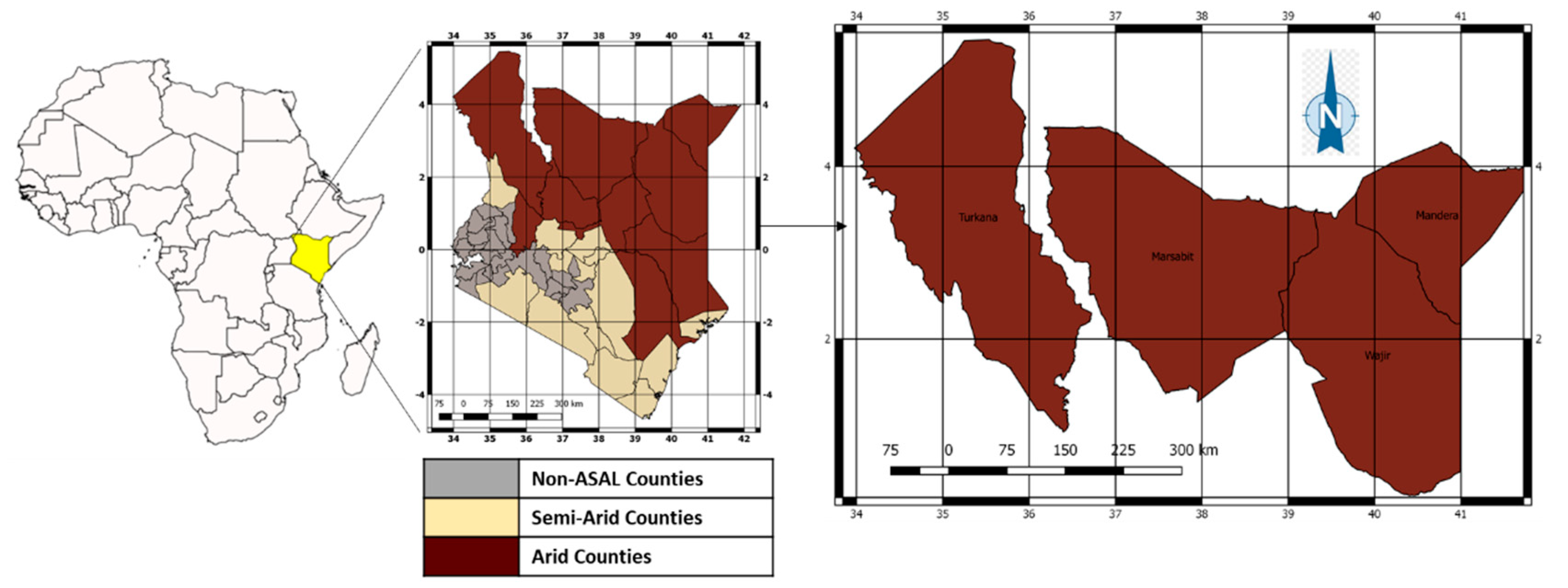
Despite the differences in the formulation of the predictive modelling steps, the main steps can be grouped into three stages: pre-modelling, model building and model deployment stages. The pre-modelling stage involves all the steps at definition of the modelling objective, data acquisition, data preparation and variable selection. The model building stage involves the formulation of multiple models, their evaluation, validation and subsequent selection. The ANN models realized from the study are computationally costly and have substantial random components. The best model was saved as an R data file to disk and executed from within Microsoft SQL server (MsSQL) which was used as the data store. In most cases, the modelling processes and stages are iterative in the search for the optimum model as provided by the best set of predictors.

2.1. Study Area

The study area is shown in Figure 2. The study area comprises four counties of Kenya: Turkana, Marsabit, Mandera and Wajir. The selected region lies in the northern part of Kenya, which is characterized as part of the arid and semi-arid lands (ASALs) of Kenya. The selected counties are classified as arid and part of the ASALs monitored by the National Drought Management Authority (NDMA) of Kenya. The four counties cover a combined area of 215,242 km2 with a total population of around 2.8 million. The annual average rainfall is 250 mm (Turkana, Marsabit and Mandera) to 370 mm (Wajir). Rainfall patter is bimodal with the long rains in March, April and May (MAM) and the short rainy season between October, November and December (OND) with 6 months considered wet months. The monthly average NDVI for the period 2003–2015 from the NDMA’s operational drought monitoring system, is shown in Figure 3. The low values indicate sparse vegetation cover, even during the wettest months (e.g., May and December).

2.2. Modelling Scheme

2.2.1. Pre-Modelling

The dataset for the study as documented in Klisch and Atzberger [22], was realized from the cooperation between BOKU and the NDMA. The data is used in an operational setting at the NDMA with statistics on drought generated monthly with an option for on-demand processing.
The variables used in this predictive study (Table 1) comprises both precipitation and vegetation indices. Moderate resolution imaging spectroradiometer (MODIS) at 250 m ground resolution is the source of the vegetation data, while Tropical Applications of Meteorology using SATellite (TAMSAT)’s version 3 product [38] is the source of the precipitation data. Both the precipitation and vegetation data are directly provided by BOKU [22]. BOKU does only post-processing (for example spatial sub-setting and temporal aggregation) on the TAMSAT data.
The vegetation datasets were smoothed using a modified Whittaker smoothing algorithm. For operational monitoring, the indicators and indices calculated at pixel level are then aggregated over the administrative units of interest at either 1 or 3-month time steps. In addition, uncertainty modeling is provided at each time step for each pixel or the MODIS derived vegetation data. The details and formulae for the computation of these indices are as provided in Table 1. The precipitation includes RFE, RCI and SPI. Vegetation conditions are characterized through NDVI and VCI.
Klisch and Atzberger [22] and Meroni et al. [40] document the use of the VCI as a temporal and spatially aggregated anomaly of the NDVI. While the NDVI gives absolute vegetation status for a given spatial extent at a given time, the VCI scales the actual NDVI value in the range between a historical minimum (VCI = 0%) and maximum (VCI = 100%) for a given time unit. Widely used time units are dekads (10-day periods), months and seasons (3 months). The choice of and the definition of drought conditions using the VCI3M is two-fold. First, the VCI as a variable is appropriate for monitoring vegetation conditions. The northern parts of Kenya are mainly pastoral lands, therefore pasture conditions and their monitoring remains key. Second, the VCI is a direct measurement, as opposed to say RFE, which is a modelled output. Several studies have evaluated the BOKU dataset including comparisons against similar products [40,41].
The input data for this study could suffer various errors. Noise as a result of cloud cover and other atmospheric disturbances is one such source of error. The data pre-processing stage of the BOKU datasets as provided in Klisch et al. [42] however mitigates this through Whittaker smoothing, which uses the vegetation indicator (VI) usefulness quality indicator in the data smoothing process. In addition, the BOKU vegetation input data are NRT and have an element of forecasting that makes the input prone to estimation errors. This is however mitigated by the use of a constrained NRT filtering approach. The precipitation data from TAMSAT potentially could suffer estimation errors arising from a limitation in the spatial distribution of in situ observation gauges at the point of historical calibration.
Drought events are defined in-terms of VCI3M for each administrative unit. The variables, with the exception of the variable ‘Month’, were lagged at 1–3 month time steps for each county to ensure that the lagged variables conform to the time series data for each county. The non-lagged variables were then dropped from the study, with the exception of VCI3M, which is the dependent variable. The resultant dataset is as described in Table 2.
Random sampling is used to partition the data into training and validation datasets. The partitions follow on the 70:30 rule for training and validation data sets, respectively.
To support decision making processes, products of operational drought monitoring systems should be easy to interpret. For example, readability of maps is improved by reducing the real value outputs to a few classes. The classes are generally subjective and are adjusted in operational systems based on practical applications. This study adopts the drought classification in Table 3 as used in Klisch and Atzberger [22], Meroni et al. [40] and Klisch et al. [42]. Even though the classes might appear subjective, the process for realizing them as documented in Klisch et al. [42] was validated retrospectively and shown to be fit for purpose in the capture of the documented drought years (2006, 2009 and 2011).

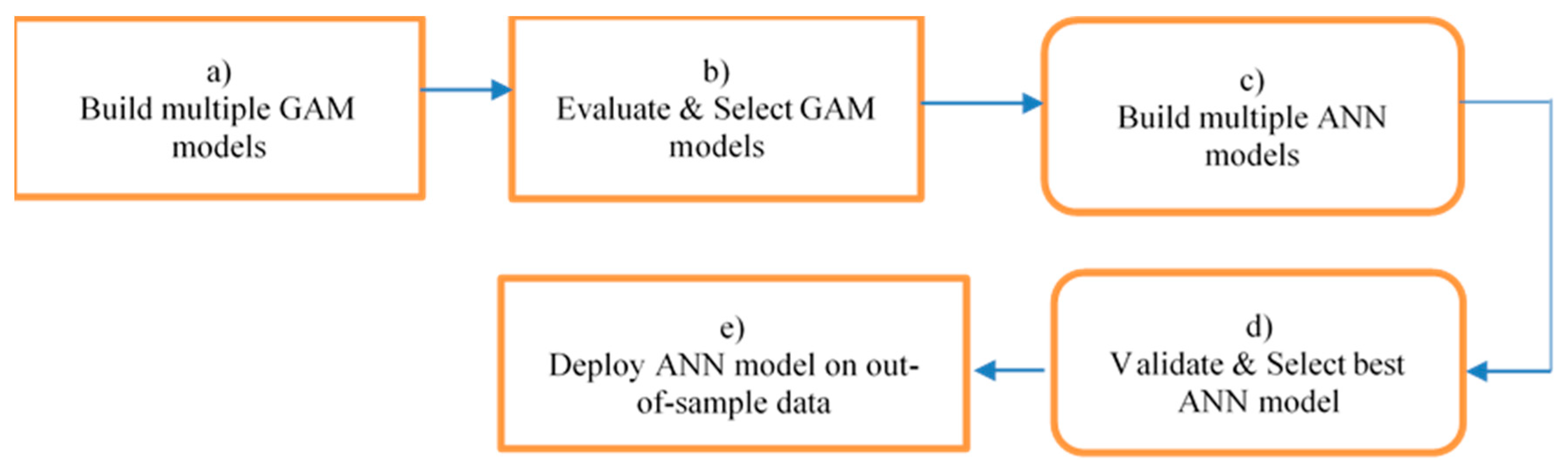
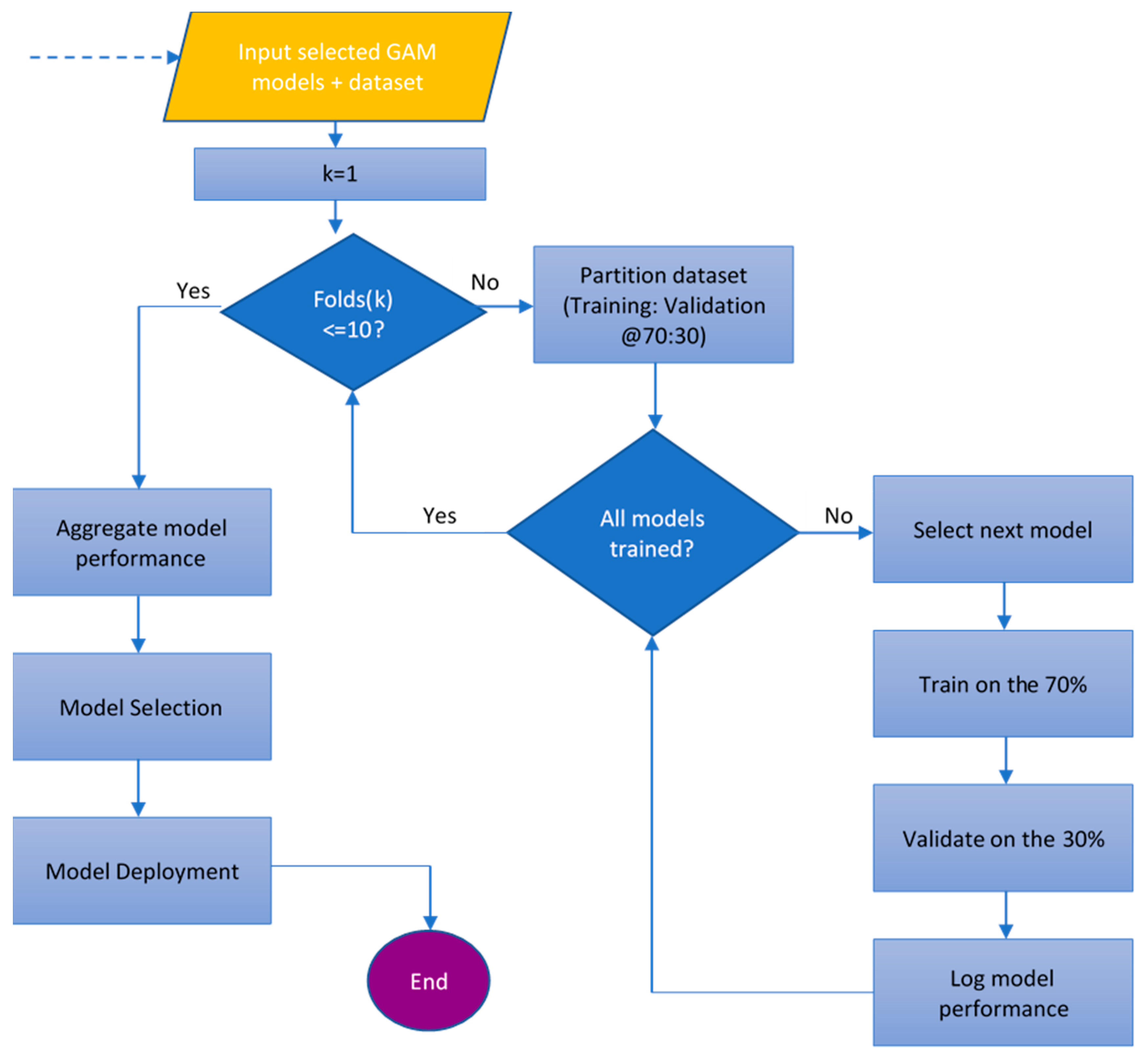
2.2.2. Model Building

The study uses multiple indices and combines two techniques in the prediction of drought. The prediction of drought is, for operational purposes, formulated as the prediction of future VCI3M values using the predictor variables presented earlier (Table 2). We focus here on predictions 1-month ahead, while 2-month and 3-month predictions ahead were also tested for the GAM process. Two approaches are combined (Figure 4):
  • A statistical approach–generalized additive models (GAM), and
  • Artificial neural networks (ANN).
GAM models are used to arrive at the set of models that offer the best predictions. These set of variables are then used to build ANN models. GAM models are thus used for model space reduction in a set-up similar to variables selection prior to subjecting the chosen models to the ANN modelling process. GAM models are reviewed for example in Hastie [43] and a good description of ANNs is provided in Ramos and Martínez [44].
The modelling process in Figure 4 is automated using scripts written in the free statistical computing R software developed by the R Core Team. The inputs into and outputs out of the R script are provided as comma separated value (csv) files. Each of the models and their parameters are serialized and saved to disk for making predictions on new data. The two modeling techniques (GAM and ANN) are described below in detail.

General Additive Models

The GAM technique was selected because it does not assume linearity between the predictor and the response variables [43]. In addition, GAM is free form and does not require the ascertainment of the functional form of the relationship and has the ability to model complex non-linear relationships, even in the presence of multiple predictors. This makes GAM models a viable tool for weather-based data modelling which exhibits non-linearity in the relationship between predictors and dependent variables. GAM models are expressed as shown in Equation (1).
Y = a + f 1 ( x 1 ) + f 2 ( x 2 ) + + f n ( x n ) + ε
where a is an intercept and f are smooth functions; Y is the response function and x1 to xn are the n predictor variables.
Smoothing functions are either local linear regression (loess) or splines. In practical application, caution is advised, since smoothing generally leads to model overfitting.
The model space for the study, as given by Equation (2) is around 2.15 billion. This space would be impractical to navigate in the search for the best predictor model.
r = 1 31 n ! ( n r ) ! r ! 2.15   b i l l i o n
To minimize the space complexity, we make some prior assumptions to avoid the futility of bias-free learning and also follow Occam’s razor [45]. First, we assume that a maximum of two variables in the GAM models will give us reasonably simple models while still remaining predictive. Second, we assume that including multiple variables of the same category (vegetation or precipitation) is an unnecessary increase of the complexity of the model space at marginal possible increased performance. Together with these two assumptions, we further use a rule of thumb to not use different lag times of the same variable in a single model. To capture seasonality, we further include an additional variable for the month of the year of the instances as a sine wave. Seasonality is expected to exist in precipitation and vegetation cover data. The month was added as an extra variable to the model formula for each GAM model as a smoothed sine function of the month number. The smoothing uses cyclic cubic regression splines (cc) that has start and end points and is thus appropriate for modelling seasonality. These assumptions achieve a reduction of the model space from an initial 2.15 billion to 102 models. With the model space reduced, we brute-forced the process of training and evaluating the models in an automated process. Multiple model evaluation metrices were used and the results logged for both model training and model evaluation. Results are reported separately for training and validation data.

Artificial Neural Networks (ANN)

ANN are a machine Learning (ML) approach that mimic the interconnectedness of the brain in the modelling process [45]. ANNs have several characteristics making them suitable for the purpose of predictive modelling; (i) instances can be represented by many attribute value pairs; (ii) the target function is either discrete, real or vector valued; (iii) training examples may contain errors; (iv) non-linear relations can be modelled, and; (v) execution (after training) is very quick.
To avoid overfitting, which is the most common limitation of ANNs, we chose models that were not judged overly to lose performance in the evaluation datasets as compared to the training datasets using R2 as the measure of model performance. Our working definition of overfitting is presented in Equation (3) and implies a loss of more than 3% in performance between training and validation is deemed as overfitting.
O v e r f i t m o d e l = { Y e s , d i f f ( R s q u a r e d T , R s q u a r e d V ) > 0.03 N o , o t h e r w i s e
where RsquaredT indicates the R2 in training set and RsquaredV is the R2 in the validation set.
The ANNs were built using the back-propagation algorithm. For the limitation of complexity, the modelling process was set to have a formation of 2-5-3-1 and thus had two hidden layers that were able to learn any arbitrary function. The formation was realized from both a rule of thumb and an experimentation process. The rule of thumb is based on Equation (4) from Huang [46] with m as number of output neurons and N as the number of samples to be learnt with negligibly small error. The total number of hidden nodes was thus set at eight.
N u m b e r o f n o d e s = { S q r t ( N × ( m + 2 ) ) + 2 × S q r t ( N / ( m + 2 ) , 1 s t h i d d e n l a y e r m × S q r t ( N / ( m + 2 ) , 2 n d h i d d e n l a y e r
The maximum step (stepmax) was set to 1 million iterations, which represented the maximum steps for the training of the neural network at whose attainment the network’s training process was stopped. The maximum step size was a failsafe condition for the ANNs, should the pre-selected set of hidden layers not lead to convergence majorly due to partitions in the training and validation datasets.
The process for the execution of the artificial neural networks modelling is as presented in Figure 5 and was built on normalized variables. For the ANN modeling, variable normalization was done prior to model training to ensure the input variables were all at a comparable range. The input variables were normalized by scaling each input’s data values to the 0–1 range (both end points included). The values were centered at the minimum value for each variable, then linearly scaled between the minimum and maximum values. The process for building the models (Figure 5) is automated including sample selection and the performance evaluation. Training each of the models over the 10 partitions of the data (diamond shapes in Figure 5) are the decision points in the model building process.

2.2.3. Model Evaluation

For all the models run, both GAM and ANN, the validation metrics used are mean absolute error (mae), mean squared error (mse), root mean squared error (rmse), mean percentage error (mape), and R2. Even though these measures of performance were generated, only R2 is presented in the results. The evaluation of the performance of the models is done as part of the model training process using the validation dataset and also using the out of sample dataset.

3. Results and Discussion

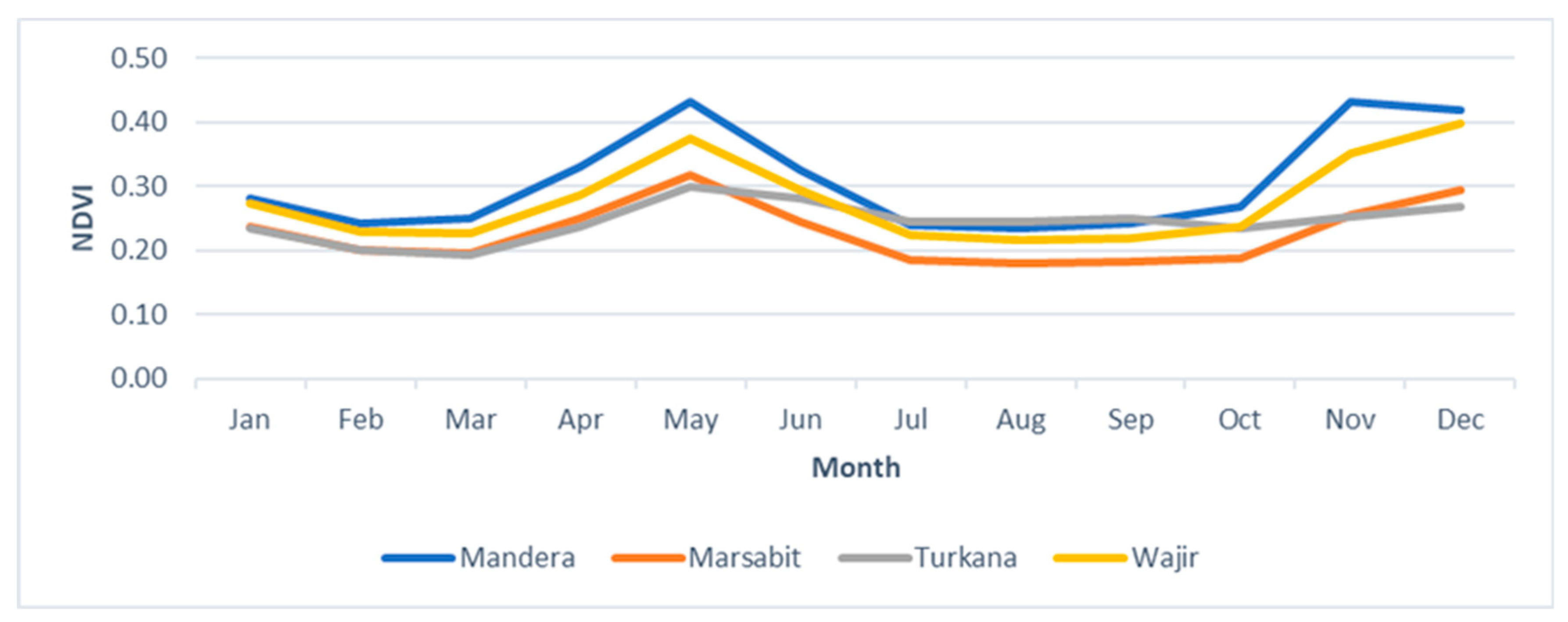
3.1. Analysis of Past Drought Events

The occurrence of drought episodes, based on the classification of Vegetation Condition Index aggregated over 3-months (VCI3M) as the proxy variable for drought conditions is shown in Table 4. The thresholds used are documented in Klisch and Atzberger [22], Meroni et al. [40] and Klisch et al. [42].
Over the 178 months period, 377 out of a possible 712 (52%) drought episodes are reported at county level, 29 (4%) of which are classified as extreme (VCI < 10) and are therefore signaling a possible collapse of community coping capabilities.

3.2. GAM Model Results

A plot of the performance of the 102 models in the GAM process, grouped by R2 is presented in Figure 6. The models are noted to post R2 between 0.09 and 0.86 in model training and model validation. The performances of the models in training and validation datasets (blue and orange bars respectively) indicate relative stability in model numbers across the models.
The performance of the models by the lag-time of the variables (between 1- and 3-month lags) is provided in Figure 7. As expected, the analysis of the GAM process by lag time indicates that the 1-month lag of the predictors perform better in predicting VCI3M as used to define drought (in green). While a lag time of 2 month (in blue) still has some predictive power (R2 > 0.5), even longer lags fail to produce good correlations (in yellow).
It is deducible that the GAM process models with R2 ≥ 0.7 (Table 5) are all 1-month lag variables. In fact, the first 2-month lag variable first appears at a model ranked at position 22 with an R2 of 0.61 while the first 3-month lag variable is in a model ranked at position 52 with an R2 of 0.33. The poor performance of higher lags of these variables is expected, since longer lags are contributing less to current vegetation status and the chances of unexpected climate variations occurring between time of forecasting and the forecasted event increasing.
With the definition of overfitting based on Equation (3) presented earlier, it is shown that none of the 21 GAM models were judged to have suffered over-fitting. All the 21 models are thus noted to have acceptable deterioration in performance in validation.
The alternative measures of performance (MAE, MSE, RMSE, MAPE, NMSE and NAME) are noted to be consistent with R2 since they all have a non- monotonic and non-linear relationships (not shown). An increase in R2 translates to a change, but in reverse direction of the other measures of model performance. The use of the GAM modelling process for model space reduction resulted in the selection of the above 21 models were selected for the ANN process.

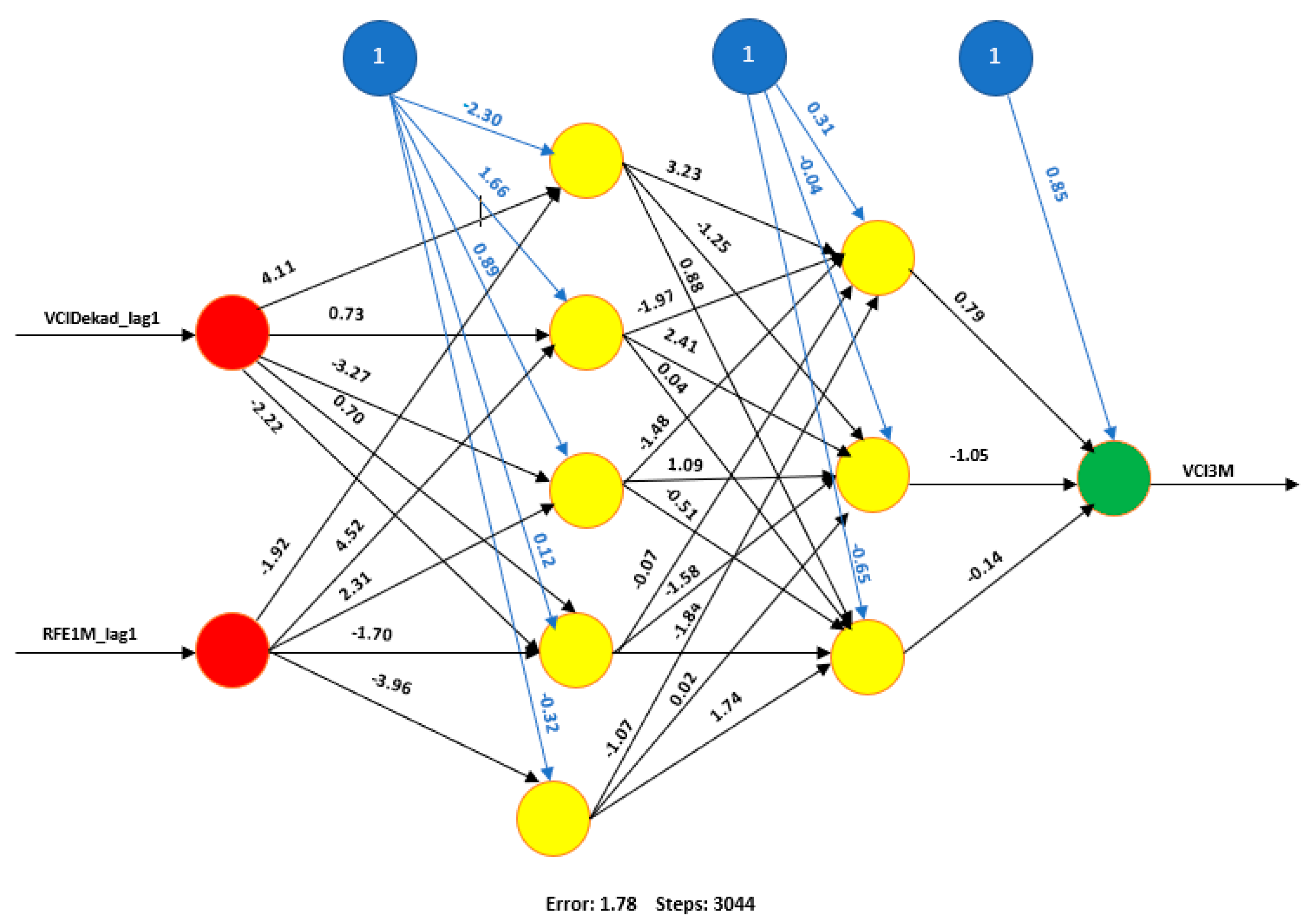
3.3. Artificial Neural Network Model Results

The study uses the ANN as the example technique of choice. Following on the model space search approach, we produced all the 21 models using the ANN process through a bagging and brute force approach in the search for the best model. For uniformity, overfitting is defined for ANN as in GAM models.

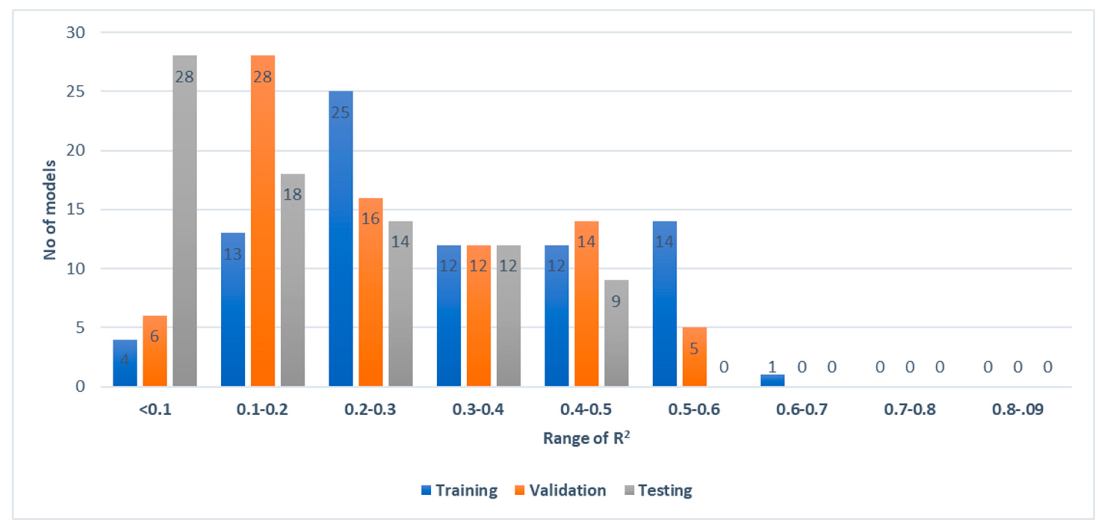
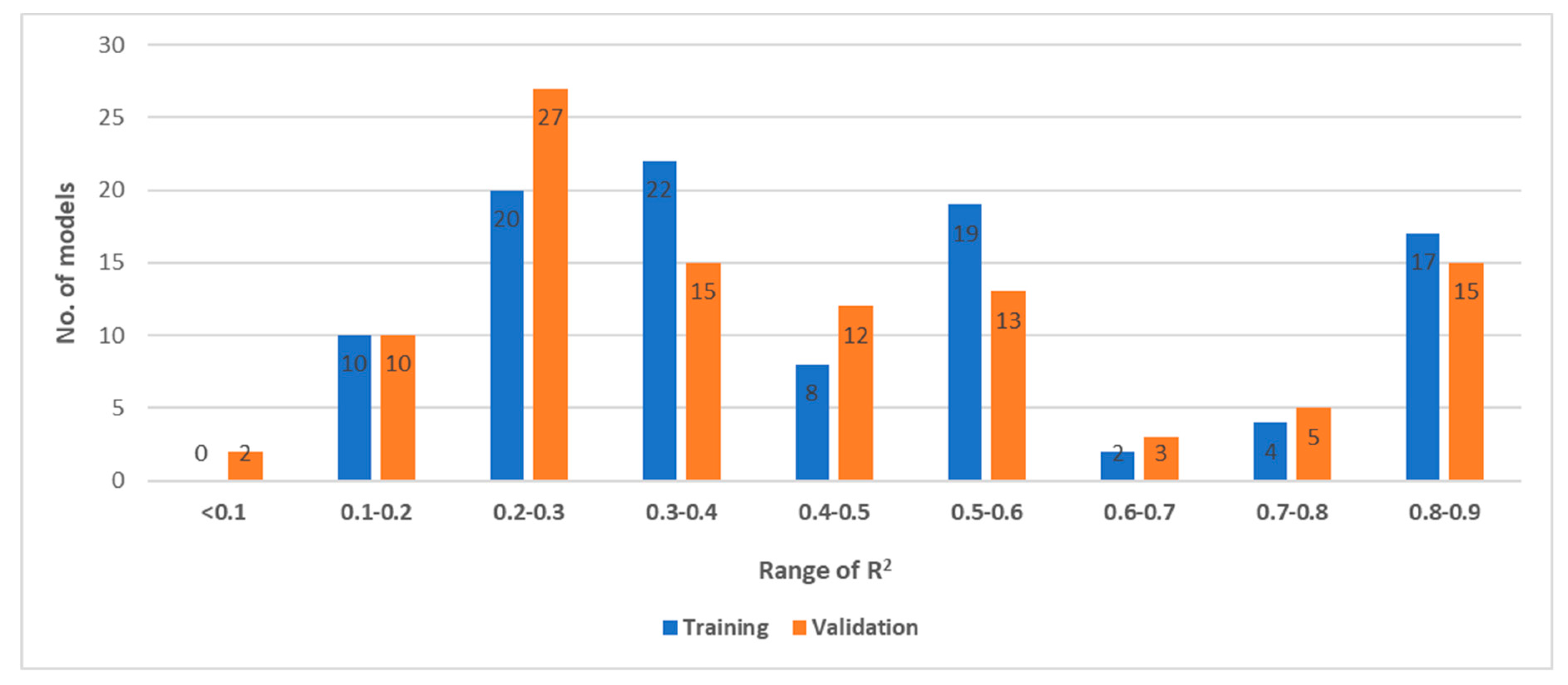
3.3.1. Artificial Neural Network Performance in Training and Validation

Using the model overfit index (Equation (3)), it emerges from the results (Table 6) that the ANN models are generally not overfit except for only one model (No. 19) that is overfit. This implies a non-overfit rate of 95%.
Since the methodology used runs the same ANN model across 10 different partitions of the training data, a review of model results indicates that almost all the models post an R2 of at least 0.7 in all the partitions of the training data except for two models (No 20 and 21 in Table 6). Model 21 from the GAM process that was earlier marked as a special case (with lag of the dependent variable) is shown to post a low performance (R2 = 0.66) in the ANN process. The best model from the ANN process is different from that of the GAM process. In fact, the best ANN model (R2 = 0.83) (No 1 in Table 6) was ranked the third best model in the GAM modelling process in Table 5 (R2 = 0.85). Figure 8 illustrates the performance of the ANN models as compared to the GAM models.
In general, as indicated in Figure 8, the GAM models outperform ANN models except for model 16, for which the ANN slightly out-performs GAM by an R2 of 0.01. This is an important property since the GAM process is proved to be more optimistic in performance as compared to ANN, and therefore fewer deserving models would be excluded from the ANN process. In the training and validation, the best ANN model has the best subset performance of R2 = 0.86 as shown in Figure 9.
A detailed analysis of the lag-time performance of the ANN models in model training is provided in the Appendix A which has the results for the 102 possible ANN models similar to the GAM process.

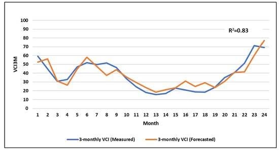
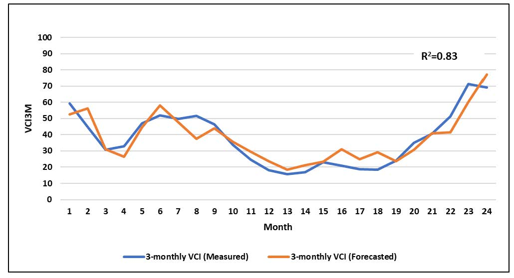
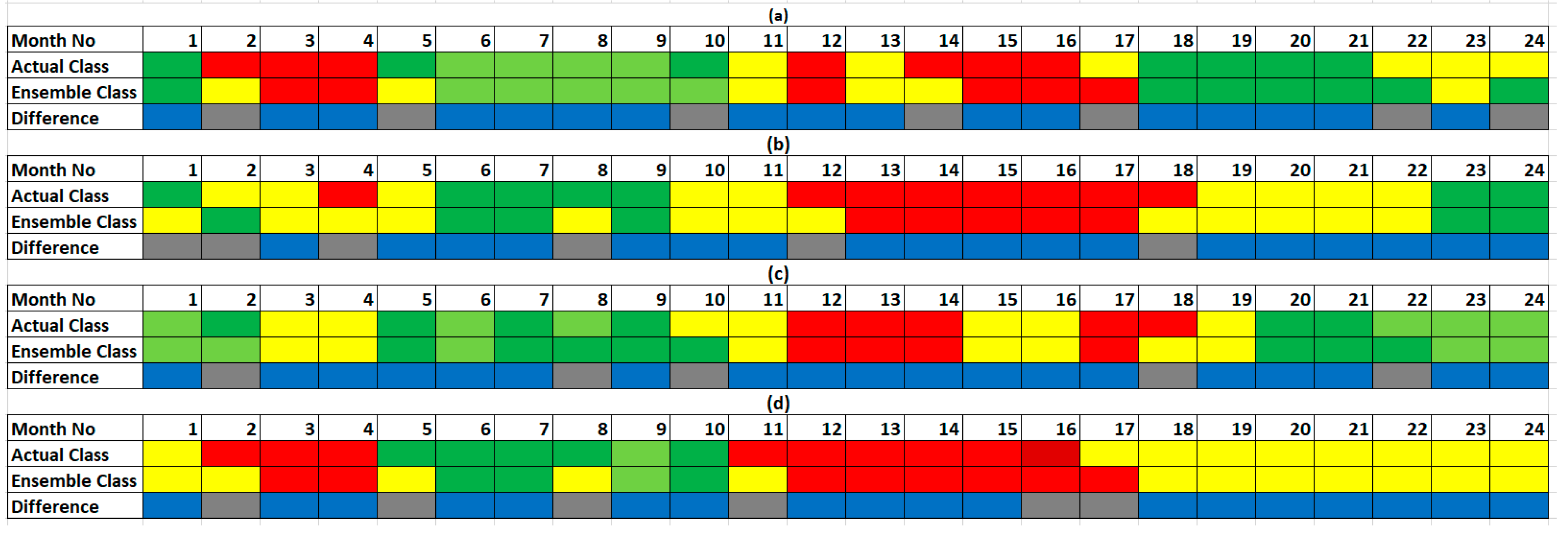
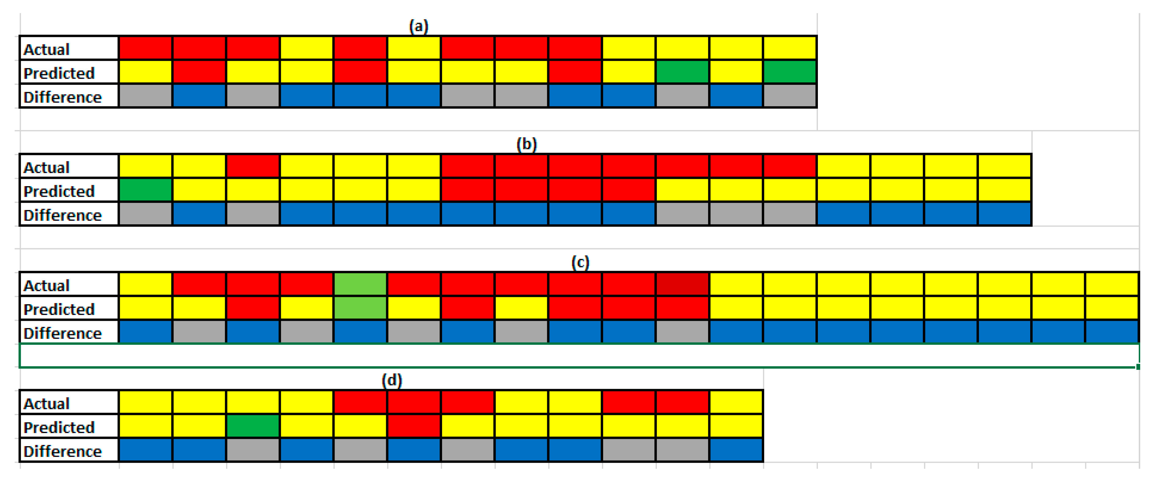
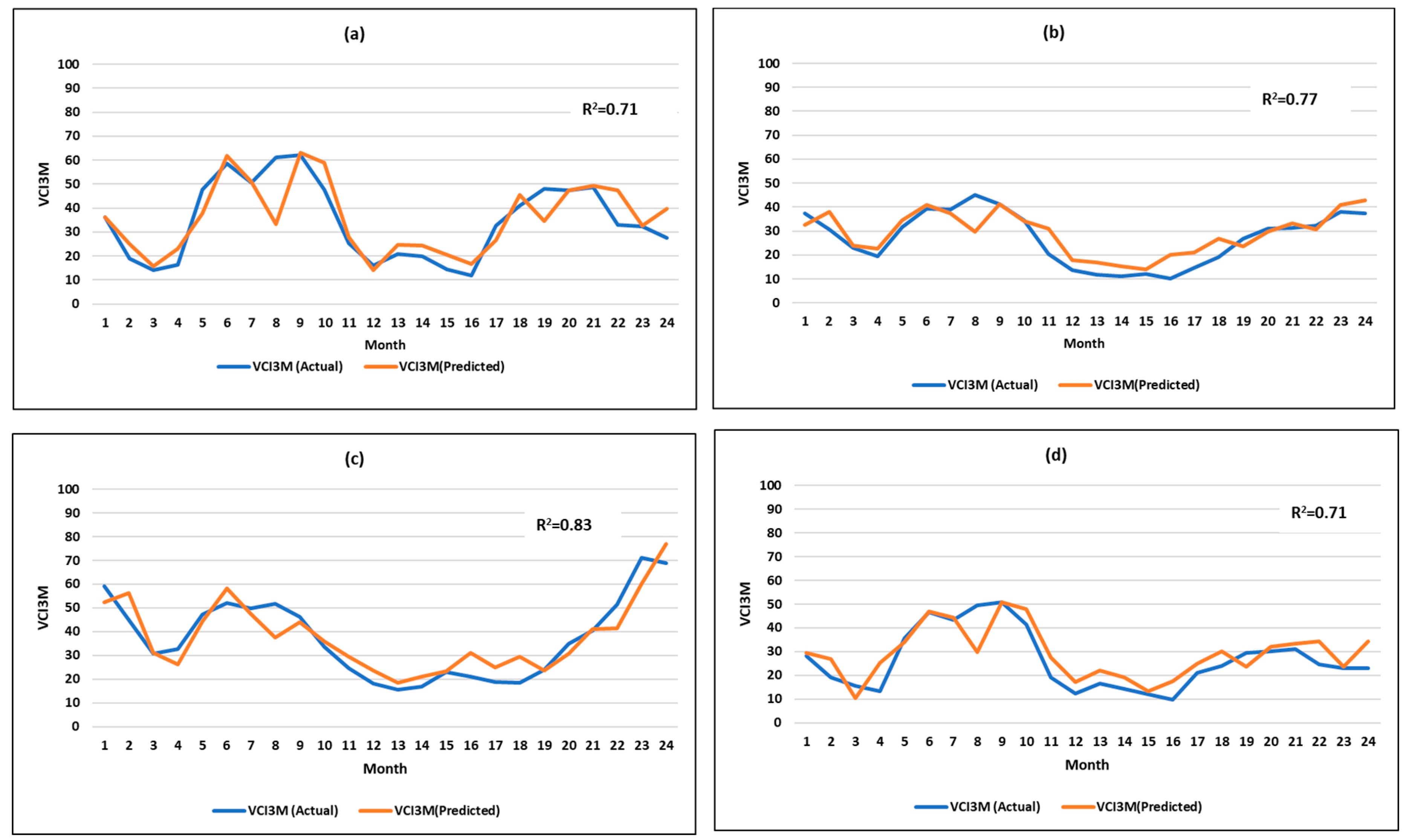
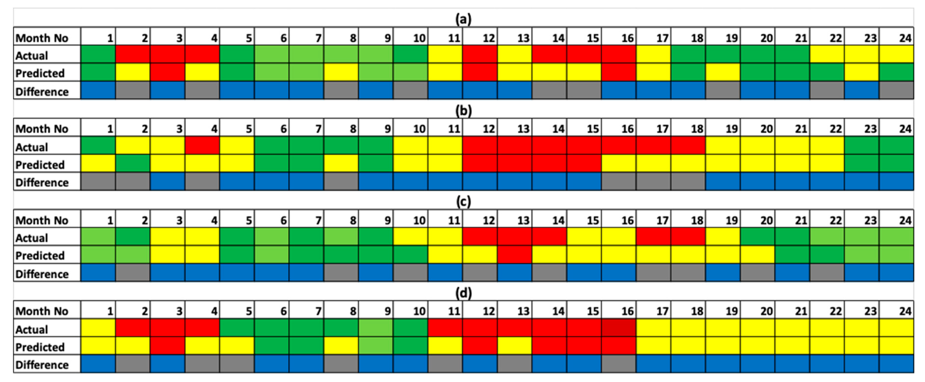
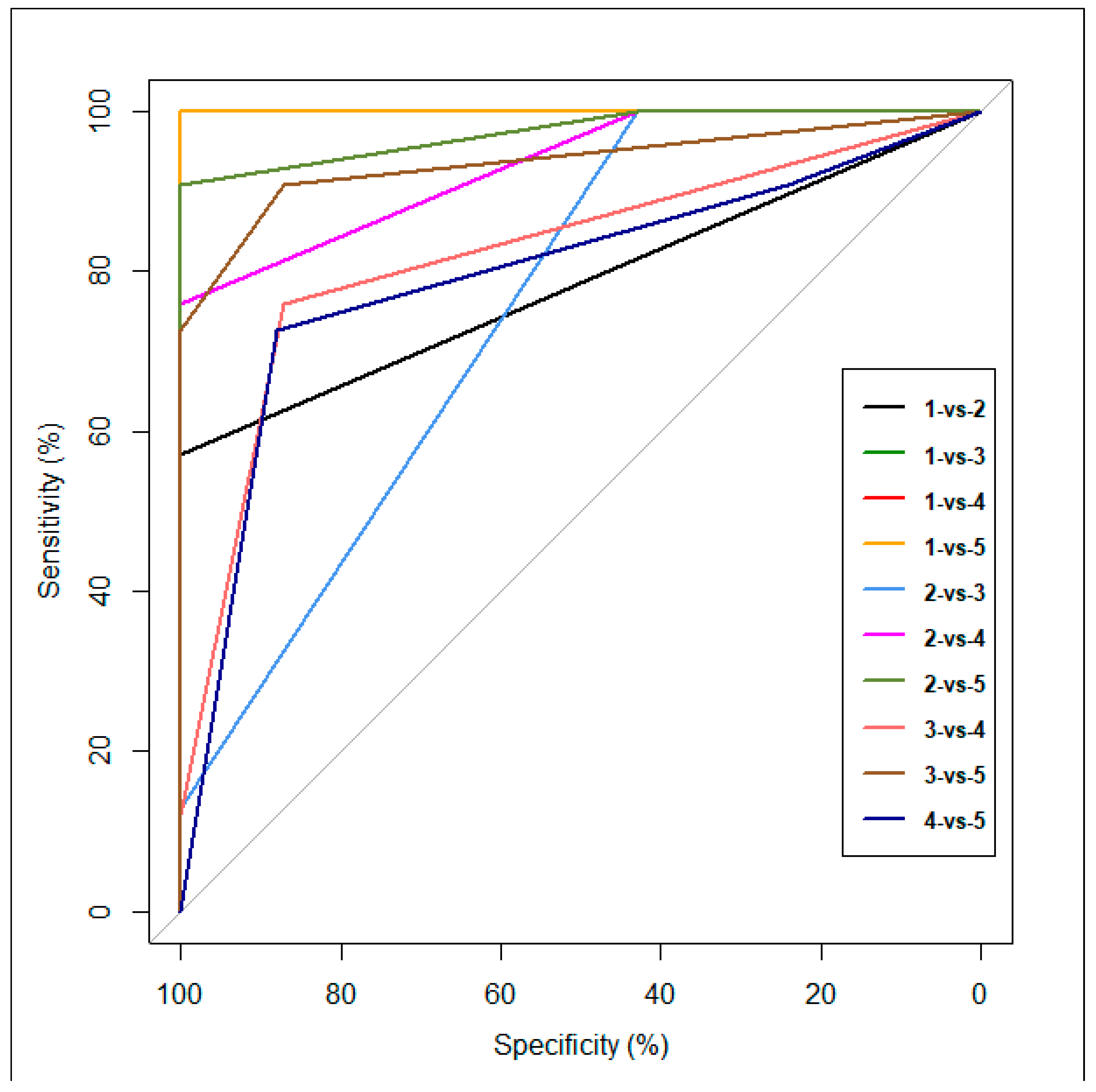
3.3.2. Performance of the Best ANN Model in the Test Dataset

The out-of-sample test dataset has 96 data points across a 2-year period. The out-of-sample data was neither used in the training nor the validation processes of the ANN and even of the GAM process. It represents the model’s performance in the real world. We describe the performance of the best ANN models both as a regressor and as a classifier.
Performance of ANN in Regression: the ANN prediction was formulated as a regression problem. The performance of the best ANN model in regression is indicated in the plot of the actuals versus the predicted real values for all the counties ordered by county and time period as shown in Figure 10.
The plot of the actual versus the predicted values represents quite a good agreement. In the test data, the best model posted an R2 of 0.78 and RMSE of 7.03 on the actual data values. The above performance over the 96 data points for testing is an acceptable performance in the prediction of drought events.
Performance of ANN in classification. Operational drought monitoring involves the definition of thresholds on indices used for drought monitoring so as to realise a phase approach to drought monitoring. We use the approach documented in Klisch and Atzberger [22], Meroni et al. [40] and Klisch et al. [42] and earlier presented in Table 3 to classify drought in five phases.
The best model had an overall accuracy of 67% over all the counties, with the highest accuracy of 71% for Wajir and Marsabit counties as indicated in the matrix provided in Figure 11. Additional analysis of the classification performance of the model in the prediction of moderate to severe drought is provide in Appendix C with an accuracy of 54% (Mandera), 71% (Marsabit), 74% (Wajir) and 58% (Turkana).
When formulated as a multi-class classification problem and multiple receiver operating characteristic (ROC) curves plotted for each of the pairwise comparisons of the classes following on the approach in Hand and Till [47], we obtained the ROC plot in Figure 12. The multi-class area under the curve (AUROC) is the average of the 10 areas under all the ROCs. The ROC for the five classes provides a reasonable trade-off between sensitivity and specificity at an overall AUROC of 89.99%. The AUROC indicates quite a good trade-off between sensitivity and specificity and is ranked within the good performance category, as it is way above the 50%, which represents a worthless test (in gray).

3.4. Validation of the Key Assumption of the Study

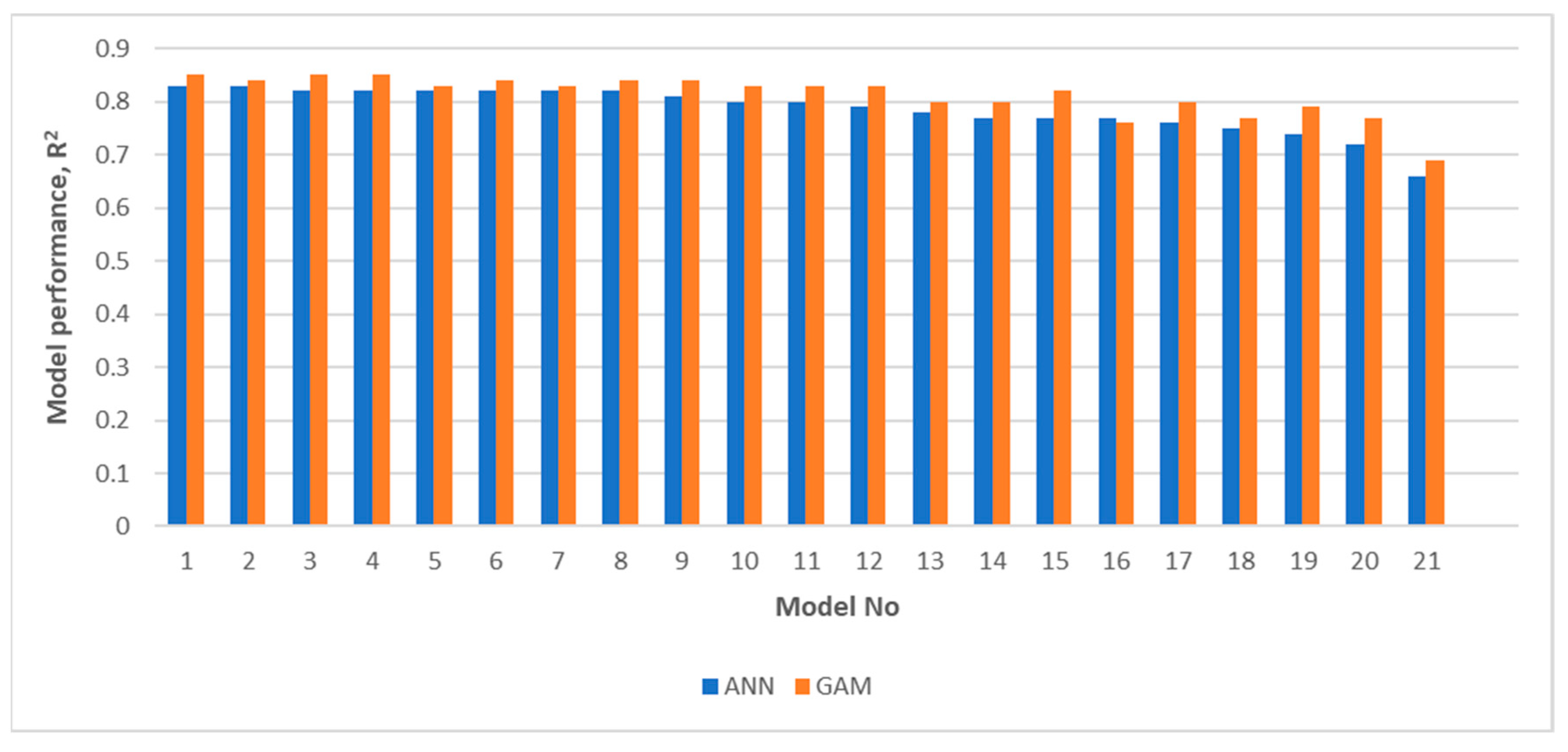
3.4.1. Appropriateness of the Use of GAM

To validate the key assumption on the appropriateness of the GAM modelling technique in the reduction of the model space, we ran the extra 81 models through the ANN process. The best performer from the set of non-selected models had an R2 of 0.50. A summary of the performance of the non-GAM selected models in the test dataset is provided in Figure 13.
The results validate the assumption of the utility of GAM in modelling non-linearity as well as in their use in this study for model space reduction prior to the use of computationally intensive algorithms like artificial neural networks. The models that are not selected by the GAM process are not expected to perform any better in the ANN process than the GAM selected models. The GAM process is, in essence, more optimistic in performance ranking than the ANN process. This property is useful as it generally guarantees that good models are not filtered out of the ANN process.

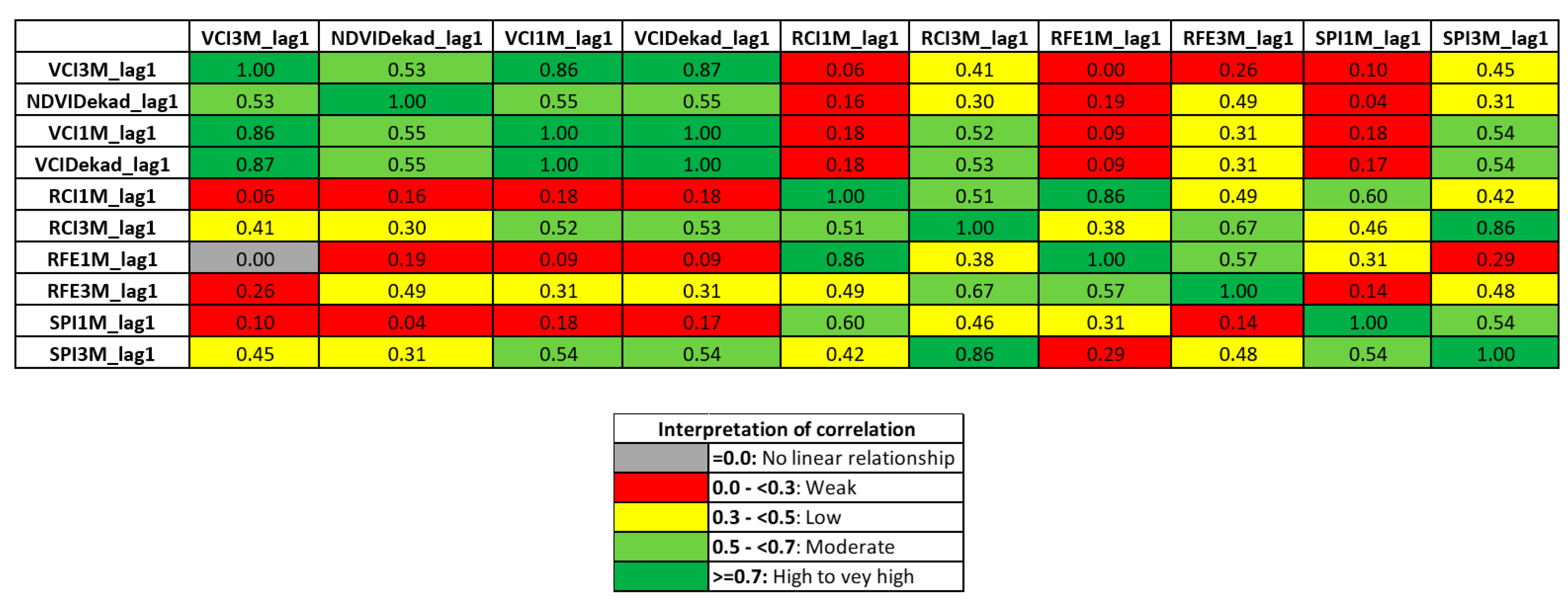
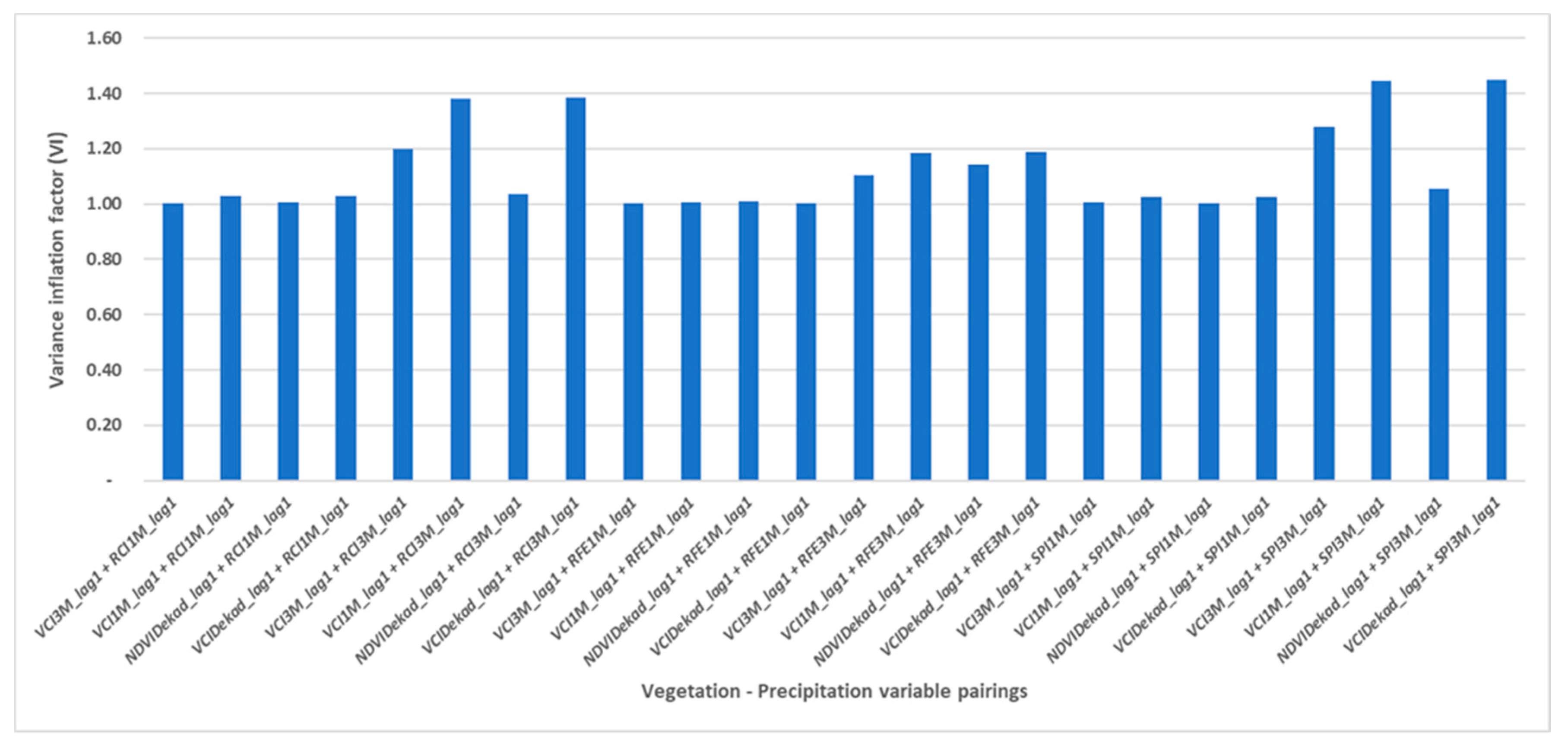
3.4.2. Investigation of Multi-Collinearity

The collinearity-matrix in Figure 14 gives the correlation coefficients between the predictor (X) variable pairs together with a proposed interpretation scheme.
From the collinearity matrix in Figure 14, the correlation between vegetation input variables is between moderate to very high correlations (min = 0.53, max = 0.87). This is as opposed to the relationship between the pairings between vegetation and precipitation datasets, which is between no linear relationship to moderate (min = 0.0, max = 0.54). The assumption to use the pairings between precipitation and vegetation datasets will therefore generally result in pairings of weak to barely moderate correlations.
In addition to the collinearity matrix, we investigated the problem of multi-collinearity between the independent variables in a two-step process—first for a model of all variables and second for the pairing of precipitation and vegetation variables. For each approach, we obtained the variable inflation factor (VIF) with the rule of thumb that a VIF > 5 indicates high multi-collinearity, while a VIF > 10 indicates multi-collinearity that has to be handled in the modeling process. The results for the investigation of VIF for all the model variables is presented in Table 7.
The full model (with all variables) indicates the presence of multi-collinearity with VIF > 10 for 2 of the predictor variables. A further analysis for the models fed in to the GAM process obtained the results provided in Figure 15.
The results in Figure 15 confirm that using the vegetation-precipitation variable pairs (corresponding to low correlation portions of the correlation matrix in Figure 14) ensures models that are not affected by multi-collinearity.
Concurvity, which has similar effects to those posed by multi-collinearity, was not a major limitation in the approach to GAM modeling employed by this study since only one smooth term was used in the development of the GAMs across all the models. In fact, an investigation with smoothing on all the terms (not presented), resulted in model overfitting that limited the smoothing of the dependent variables.

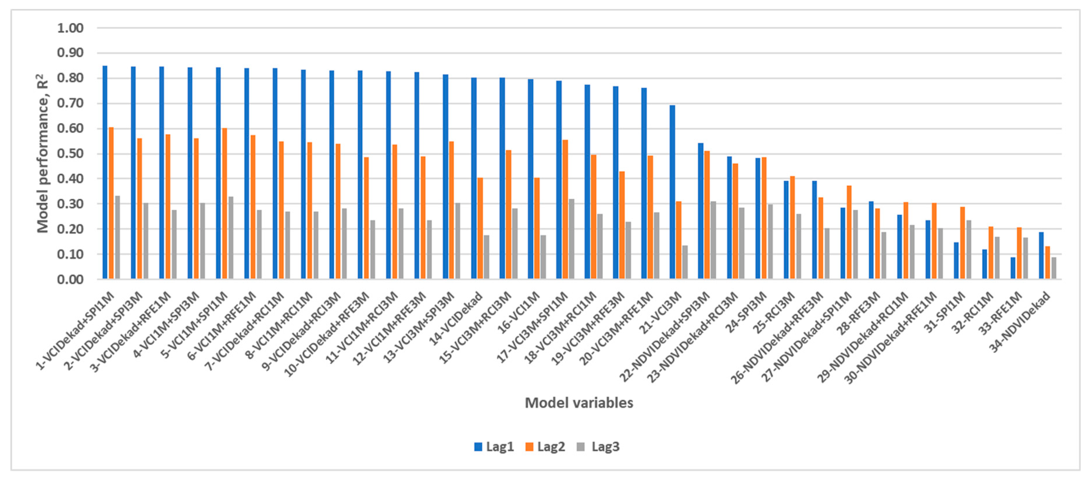
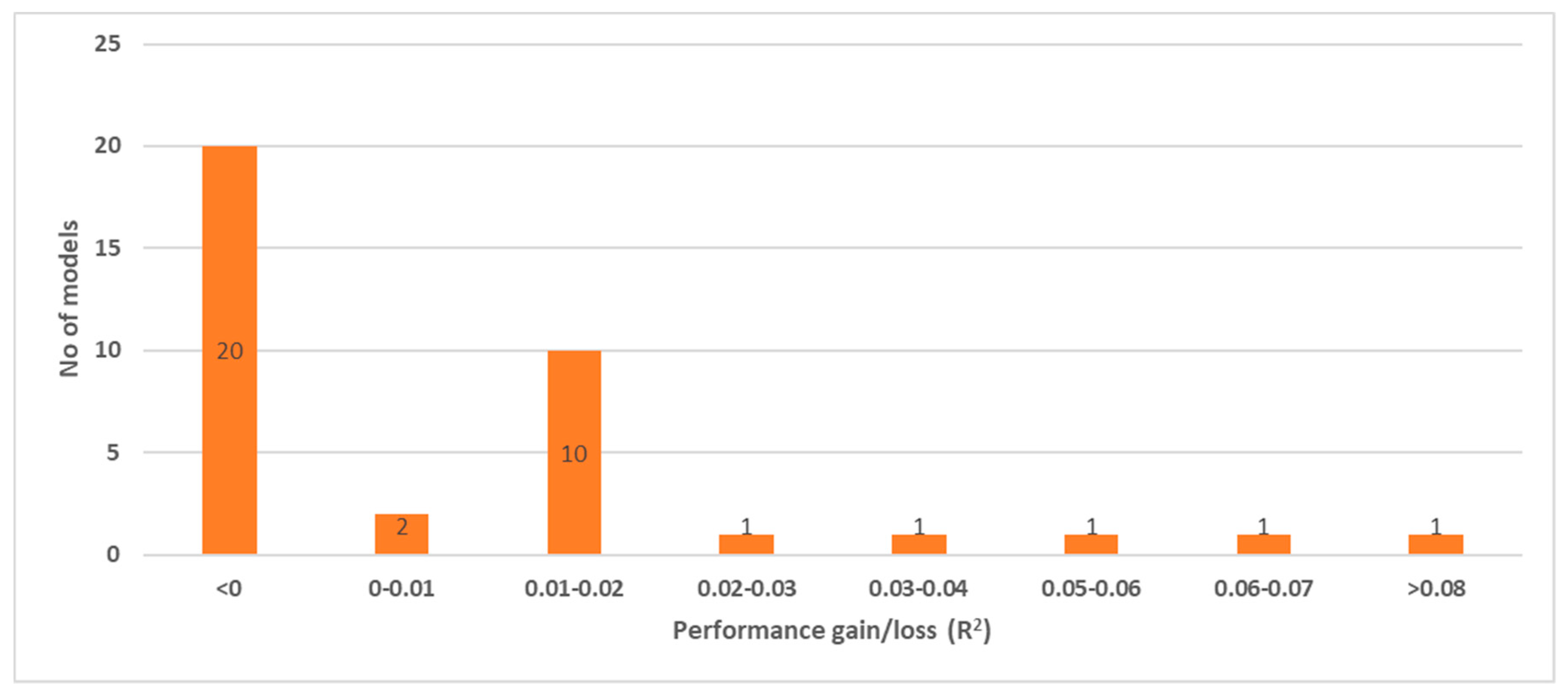
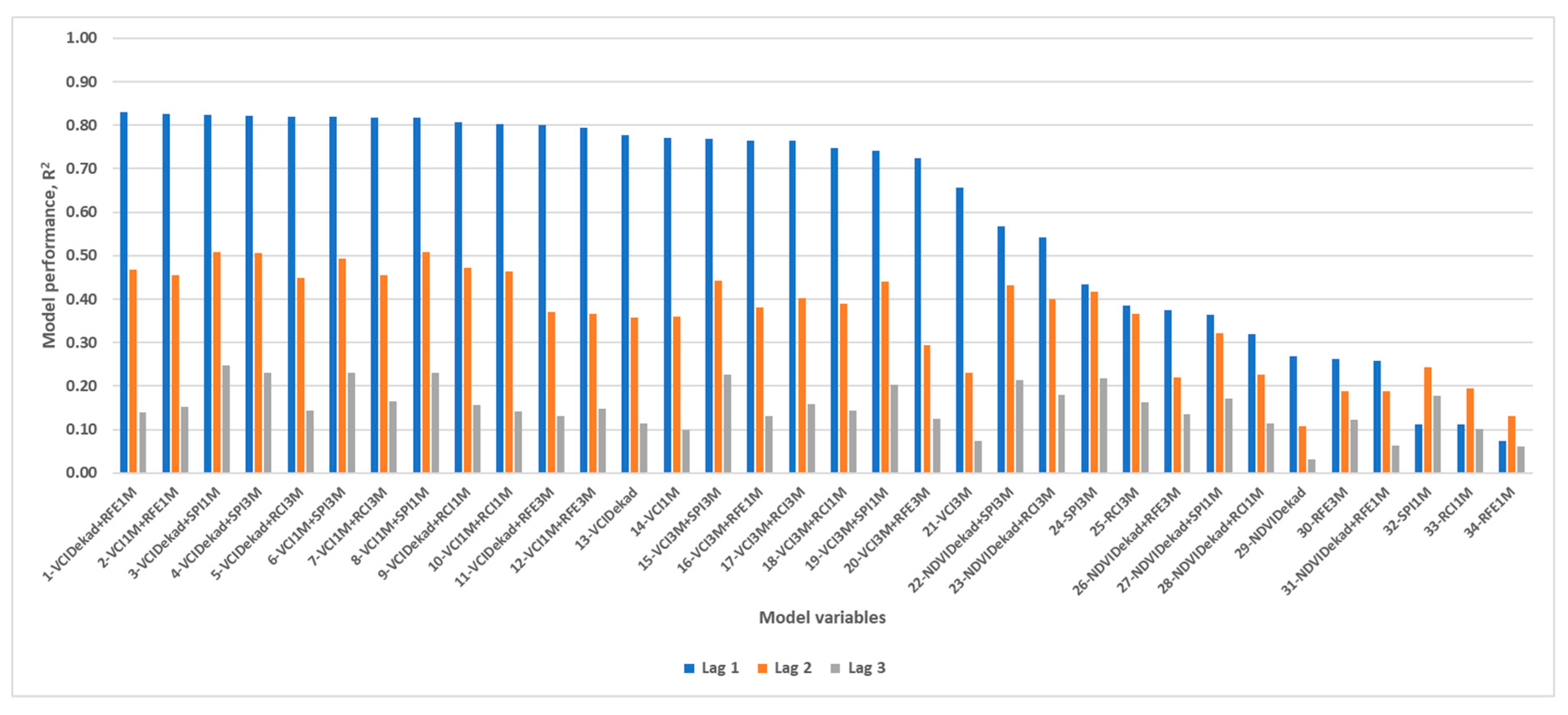
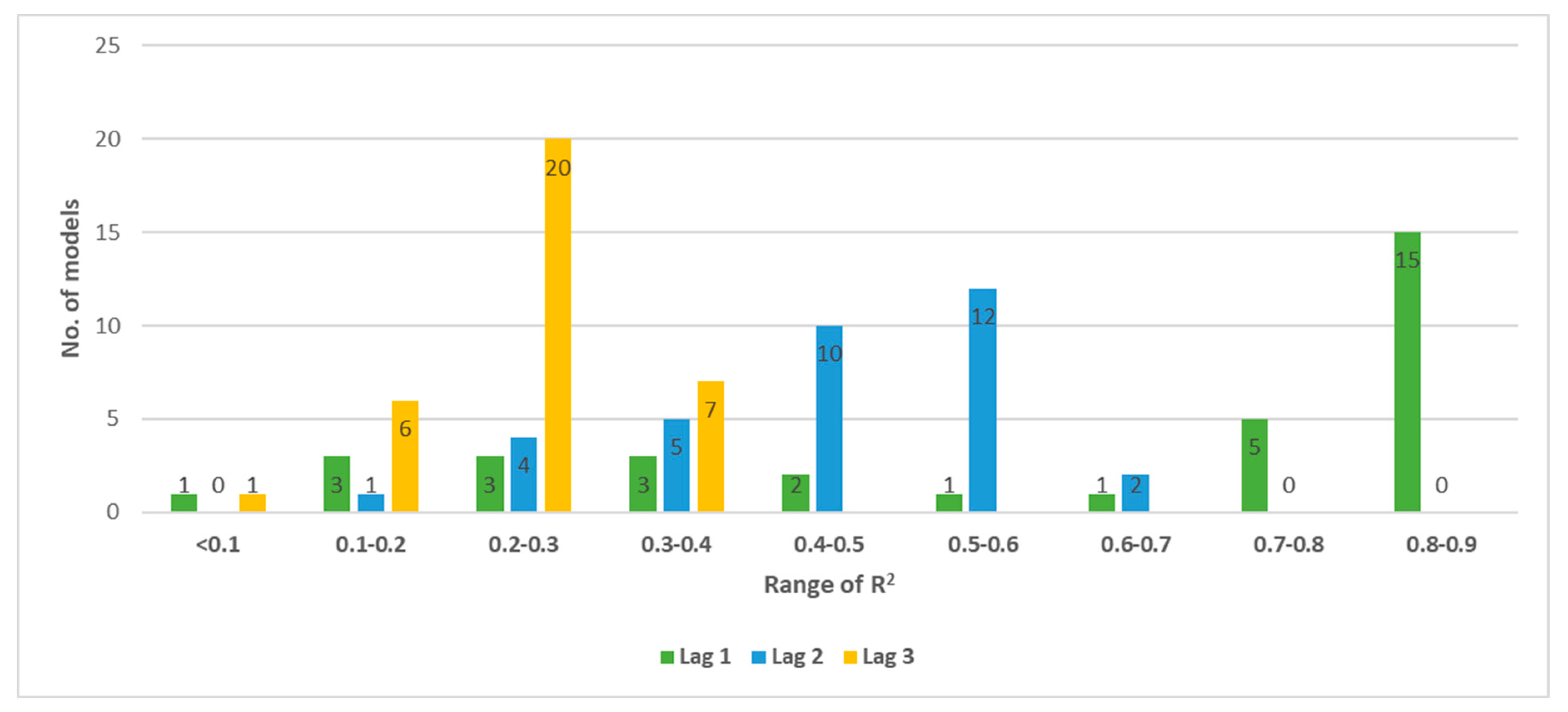
3.4.3. Performance of Models with Lags of the Same Variable

To investigate auto-correlation, we ran both VIF and performance test on the 40 possible models with lags of the predictor variables. Only three models of the possible 40 returned VIF > 5 implying multi-collinearity. Despite the results showing that the lags for the same variable can be used in the same model for the balance of 37 models, an actual investigation of their performance, as provided in Figure 16, provides contrary evidence.
Only 17 models post a gain in performance of 1% or more. All the models that post an R2 of at least 0.5 either have a loss of 6% in performance to a gain of 1% implying poor return in having multiple lags of the same variable in a model.

4. Conclusions

In this paper, multiple variables were used to predict future vegetation condition index (VCI) as a proxy to drought conditions. The predictor variables were 1–3-month lags of precipitation and vegetation indices. The methodology used two techniques in a setup where the general additive model (GAM) statistical approach is first run against several possible model configurations. The GAM method is then used to reduce the model space and by extension the set of viable variables. After variable selection and with the model space reduced, a brute force approach is then employed using the artificial neural networks (ANN) approach.
One month ahead forecasts of the VCI using the best ANN model showed good performances with R2 ranging between 0.71 and 0.83. After grouping into five drought classes, 63 to 71% of the months were correctly classified—the remaining months showed a maximum difference of one class. Prediction skills deteriorated with lag times longer than 1 month. The poor performance of variables with longer times lags, in the prediction of drought events was established. Since the approach builds multiple models, prior to evaluation in the search for the best model, it is possible to support model ensembling that supports the use of multiple models in the prediction of future events.
The study demonstrated that the model space reduction is beneficial to the building of neural networks that are known to generally have slower training times as compared to other approaches. The automation of the model training and model validation processes, and the measure of performance with a view to quantifying and avoiding overfitting, make for a scalable approach.

Author Contributions

conceptualization, C.A. (Chrisgone Adede); formal analysis, C.A. (Chrisgone Adede); investigation, C.A. (Chrisgone Adede); methodology, C.A. (Chrisgone Adede), R.O., P.W.W. and C.A.; supervision, R.O. and P.W.W.; validation, R.O., P.W.W. and C.A. (Clement Atzberger); visualization, C.A. (Chrisgone Adede); writing—original draft, C.A. (Chrisgone Adede), R.O. and P.W.W.; writing—review & editing, C.A. (Clement Atzberger).

Funding

This research received no direct external funding. The data used in the study was however, partly funded by the European Commission’s funding under a grant contact to the Institute for Surveying, Remote Sensing and Land Information, University of Natural Resources and Life Sciences (BOKU).

Acknowledgments

Our appreciation to the National Drought Management Authority for providing the data from the operational drought monitoring system. We are also grateful to Luigi Luminari for the continued discussion of the ideas of the paper towards shaping it to have outputs applicable in an operational drought monitoring environment. The help from Maquins Sewe especially with plotting in R cannot go unmentioned. The helpful contributions of the editors and reviewers are also acknowledged.

Conflicts of Interest

The authors declare no conflict of interest.

Appendix A

The study built 102 models in the general additive model (GAM) process. The models were for 1,2 and 3 month lags on of 34 unique model variables. We present the analysis of the lag time performance of the GAM and ANN approaches, assuming the case that the ANN method was also run on the complete set of models.

Appendix A1. GAM Model Performance by Lag Time

The comparison of the lag-based performance of the GAM models ordered by their performance in 1-month lag is provided in Figure A1. A summary of the descriptive statistics of the models based on lag time is presented in Table A1.
Figure A1. Lag-based performance of the GAM models. The 1-month lags are in blue lines, the 2-month lags in orange lines and 3-month lags in grey.
Remotesensing 11 01099 g0a1
The models build using 1-month lag variables are shown to perform better than the 2-month and 3-month lags except in 8 out of the 34 cases when 2-month lag time models outperform the 1-month lag models. Even in these 8 cases, the performance of the 2-month lags are still below R2 of 0.5.
Table A1. Summary of GAM model performance by lag time.
StatisticLag1Lag2Lag3
Mean0.620.440.25
Median0.780.490.27
Range0.760.470.24
Minimum0.090.130.09
Maximum0.850.610.33
From Table A1, a summary of performance of all the GAM models shows that 1-month prediction has the best performance as compared to the 2-3 months prediction ahead. Despite posting the highest range, 1-month predictions still post a mean performance of R2 = 0.62 as compared to 0.44 and 0.25 for 2-month and 3-month lag times, respectively.

Appendix A2. ANN Model Performance by Lag Time

The study proceeded, in the test of assumptions, to run the ANN process on the entire set of models in the ANN process. A summary of the results is provided following on the same set as the GAM models.
In training, as measured by the performance in the 30% (validation) dataset portion of the training data, the performance of the ANN models is as shown in Figure A2.
Figure A2. Lag-based performance of the full set (102) ANN models. The 1-month lags are in blue lines, the 2-month lags in orange lines and 3-month lags in grey.
Remotesensing 11 01099 g0a2
From Figure A2, it is shown that for each of the models, predictions 1-month ahead outperform those for 2-month and 3-month ahead except for the last cases three cases (models 32–34) when predictions 2-month ahead are better. At no point does any model have its predictions 3-month ahead out-perform any of the short time period predictions. A summary of the descriptive statistics of the ANN models is provided in Table A2.
Table A2. Summary of ANN model performance by lag time
StatisticLag 1Lag 2Lag 3
Mean0.600.360.15
Median0.760.380.15
Range0.760.400.22
Minimum0.070.110.03
Maximum0.830.510.25
From Table A2, is noted that predictions 1-month ahead post the highest range but still end up recording the highest mean of the lagged predictions. At an average R2 of 0.6 for all the 102 models the predictions 1-month ahead are judged predictive enough for use in an operational ex-ante system. The best model for prediction 1-month ahead differs from the best model for 2-month and 3-month ahead predictions. Both models have the variable VCIDekad while RFE for the predictions 1-month ahead and SPI1M for both predictions 2-months and 3-months ahead.

Appendix B

The full list of GAM models is presented in Table A3, while the full list of ANN models is presented in Table A4 respectively.
Table A3. GAM models in decreasing order of R2 with the overfit index provided.
NoModelR2 Training R2 ValidationOverfit IndexOverfitLag Time
1VCIDekad_lag1+SPI1M_lag10.860.850.01NoLag1
2VCIDekad_lag1+SPI3M_lag10.860.850.01NoLag1
3VCIDekad_lag1+RFE1M_lag10.850.850.01NoLag1
4VCI1M_lag1+SPI3M_lag10.850.840.01NoLag1
5VCI1M_lag1+SPI1M_lag10.850.840.01NoLag1
6VCI1M_lag1+RFE1M_lag10.850.840.01NoLag1
7VCIDekad_lag1+RCI1M_lag10.850.840.01NoLag1
8VCI1M_lag1+RCI1M_lag10.840.830.01NoLag1
9VCIDekad_lag1+RCI3M_lag10.840.830.01NoLag1
10VCIDekad_lag1+RFE3M_lag10.840.830.01NoLag1
11VCI1M_lag1+RCI3M_lag10.840.830.01NoLag1
12VCI1M_lag1+RFE3M_lag10.830.830.01NoLag1
13VCI3M_lag1+SPI3M_lag10.820.820.01NoLag1
14VCIDekad_lag10.810.80.01NoLag1
15VCI3M_lag1+RCI3M_lag10.810.80.01NoLag1
16VCI1M_lag10.810.80.01NoLag1
17VCI3M_lag1+SPI1M_lag10.810.790.01NoLag1
18VCI3M_lag1+RCI1M_lag10.780.770.01NoLag1
19VCI3M_lag1+RFE3M_lag10.780.770.01NoLag1
20VCI3M_lag1+RFE1M_lag10.780.760.01NoLag1
21VCI3M_lag10.720.690.02NoLag1
22VCIDekad_lag2+SPI1M_lag20.610.610NoLag2
23VCI1M_lag2+SPI1M_lag20.60.60NoLag2
24VCIDekad_lag2+RFE1M_lag20.580.580NoLag2
25VCI1M_lag2+RFE1M_lag20.580.570NoLag2
26VCI1M_lag2+SPI3M_lag20.570.560.01NoLag2
27VCIDekad_lag2+SPI3M_lag20.570.560.01NoLag2
28VCI3M_lag2+SPI1M_lag20.560.560NoLag2
29VCIDekad_lag2+RCI1M_lag20.560.550.02NoLag2
30VCI3M_lag2+SPI3M_lag20.550.550NoLag2
31VCI1M_lag2+RCI1M_lag20.560.550.02NoLag2
32NDVIDekad_lag1+SPI3M_lag10.560.540.02NoLag1
33VCIDekad_lag2+RCI3M_lag20.550.540.02NoLag2
34VCI1M_lag2+RCI3M_lag20.550.540.02NoLag2
35VCI3M_lag2+RCI3M_lag20.530.510.01NoLag2
36NDVIDekad_lag2+SPI3M_lag20.520.510.01NoLag2
37VCI3M_lag2+RCI1M_lag20.510.490.02NoLag2
38VCI3M_lag2+RFE1M_lag20.50.490.01NoLag2
39NDVIDekad_lag1+RCI3M_lag10.510.490.02NoLag1
40VCI1M_lag2+RFE3M_lag20.510.490.02NoLag2
41VCIDekad_lag2+RFE3M_lag20.510.490.02NoLag2
42SPI3M_lag20.490.490NoLag2
43SPI3M_lag10.50.480.02NoLag1
44NDVIDekad_lag2+RCI3M_lag20.480.460.02NoLag2
45VCI3M_lag2+RFE3M_lag20.440.430.02NoLag2
46RCI3M_lag20.420.410.01NoLag2
47VCI1M_lag20.430.40.03NoLag2
48VCIDekad_lag20.430.40.03NoLag2
49NDVIDekad_lag1+RFE3M_lag10.410.390.02NoLag1
50RCI3M_lag10.410.390.02NoLag1
51NDVIDekad_lag2+SPI1M_lag20.40.370.03NoLag2
52VCIDekad_lag3+SPI1M_lag30.350.330.01NoLag3
53VCI1M_lag3+SPI1M_lag30.340.330.01NoLag3
54NDVIDekad_lag2+RFE3M_lag20.350.330.02NoLag2
55VCI3M_lag3+SPI1M_lag30.330.320.01NoLag3
56VCI3M_lag20.330.310.02NoLag2
57RFE3M_lag10.320.310.01NoLag1
58NDVIDekad_lag3+SPI3M_lag30.330.310.02NoLag3
59*NDVIDekad_lag2+RCI1M_lag20.350.310.05YesLag2
60VCI1M_lag3+SPI3M_lag30.320.310.02NoLag3
61VCI3M_lag3+SPI3M_lag30.320.310.01NoLag3
62VCIDekad_lag3+SPI3M_lag30.320.310.01NoLag3
63NDVIDekad_lag2+RFE1M_lag20.340.310.03NoLag2
64SPI3M_lag30.310.30.02NoLag3
65SPI1M_lag20.320.290.03NoLag2
66NDVIDekad_lag3+RCI3M_lag30.310.290.02NoLag3
67NDVIDekad_lag1+SPI1M_lag10.310.290.03NoLag1
68VCI1M_lag3+RCI3M_lag30.30.280.02NoLag3
69VCI3M_lag3+RCI3M_lag30.30.280.02NoLag3
70VCIDekad_lag3+RCI3M_lag30.30.280.02NoLag3
71RFE3M_lag20.290.280.01NoLag2
72VCIDekad_lag3+RFE1M_lag30.310.280.03NoLag3
73VCI1M_lag3+RFE1M_lag30.310.280.03NoLag3
74NDVIDekad_lag3+SPI1M_lag30.30.280.02NoLag3
75VCIDekad_lag3+RCI1M_lag30.290.270.02NoLag3
76VCI1M_lag3+RCI1M_lag30.290.270.02NoLag3
77VCI3M_lag3+RFE1M_lag30.30.270.03NoLag3
78VCI3M_lag3+RCI1M_lag30.280.260.02NoLag3
79RCI3M_lag30.280.260.02NoLag3
80NDVIDekad_lag1+RCI1M_lag10.280.260.02NoLag1
81VCIDekad_lag3+RFE3M_lag30.250.240.01NoLag3
82VCI1M_lag3+RFE3M_lag30.250.230.01NoLag3
83NDVIDekad_lag1+RFE1M_lag10.260.230.02NoLag1
84SPI1M_lag30.250.230.02NoLag3
85VCI3M_lag3+RFE3M_lag30.240.230.02NoLag3
86NDVIDekad_lag3+RCI1M_lag30.240.220.02NoLag3
87*RCI1M_lag20.250.210.04YesLag2
88RFE1M_lag20.240.210.03NoLag2
89NDVIDekad_lag3+RFE1M_lag30.240.210.03NoLag3
90NDVIDekad_lag3+RFE3M_lag30.230.20.02NoLag3
91RFE3M_lag30.210.190.02NoLag3
92NDVIDekad_lag10.220.190.03NoLag1
93VCI1M_lag30.190.180.01NoLag3
94VCIDekad_lag30.190.180.01NoLag3
95RCI1M_lag30.190.170.02NoLag3
96RFE1M_lag30.20.170.03NoLag3
97SPI1M_lag10.170.150.03NoLag1
98VCI3M_lag30.150.130.02NoLag3
99NDVIDekad_lag20.160.130.03NoLag2
100RCI1M_lag10.130.120.01NoLag1
101RFE1M_lag10.110.090.02NoLag1
102NDVIDekad_lag30.110.090.02NoLag3
1 The overfit models are marked with * on the column No.
The GAM models only have two out of 102 (under 2%) of models judged as overfit. This is as compared to the ANN models in Table A4, which indicates 64 out of 102 models losing performance in validation by more than an R2 of 0.03 as compared to their performance in training.
Table A4. ANN models in decreasing order of R2 with the overfit index provided.
NoModelR2 TrainingR2 ValidationOverfit IndexOverfitLag Time
1VCIDekad_lag1+RFE1M_lag10.840.830.01No1
2VCI1M_lag1+RFE1M_lag10.840.830.01No1
3VCIDekad_lag1+SPI1M_lag10.840.820.02No1
4VCIDekad_lag1+SPI3M_lag10.840.820.02No1
5VCIDekad_lag1+RCI3M_lag10.840.820.02No1
6VCI1M_lag1+SPI3M_lag10.840.820.02No1
7VCI1M_lag1+RCI3M_lag10.840.820.02No1
8VCI1M_lag1+SPI1M_lag10.840.820.02No1
9VCIDekad_lag1+RCI1M_lag10.820.810.02No1
10VCI1M_lag1+RCI1M_lag10.820.800.02No1
11VCIDekad_lag1+RFE3M_lag10.820.800.02No1
12VCI1M_lag1+RFE3M_lag10.810.790.02No1
13VCIDekad_lag10.790.780.01No1
14VCI1M_lag10.780.770.01No1
15VCI3M_lag1+SPI3M_lag10.790.770.03No1
16VCI3M_lag1+RFE1M_lag10.770.770.01No1
17VCI3M_lag1+RCI3M_lag10.790.760.03No1
18VCI3M_lag1+RCI1M_lag10.770.750.02No1
19*VCI3M_lag1+SPI1M_lag10.780.740.04Yes1
20VCI3M_lag1+RFE3M_lag10.740.720.02No1
21VCI3M_lag10.680.660.02No1
22*NDVIDekad_lag1+SPI3M_lag10.600.570.04Yes1
23*NDVIDekad_lag1+RCI3M_lag10.590.540.05Yes1
24*VCI1M_lag2+SPI1M_lag20.570.510.06Yes2
25*VCIDekad_lag2+SPI1M_lag20.580.510.07Yes2
26*VCIDekad_lag2+SPI3M_lag20.540.510.04Yes2
27*VCI1M_lag2+SPI3M_lag20.560.490.07Yes2
28*VCIDekad_lag2+RCI1M_lag20.530.470.06Yes2
29*VCIDekad_lag2+RFE1M_lag20.520.470.06Yes2
30*VCI1M_lag2+RCI1M_lag20.530.460.07Yes2
31*VCI1M_lag2+RCI3M_lag20.530.460.08Yes2
32*VCI1M_lag2+RFE1M_lag20.530.460.07Yes2
33*VCIDekad_lag2+RCI3M_lag20.520.450.07Yes2
34*VCI3M_lag2+SPI3M_lag20.520.440.08Yes2
35*VCI3M_lag2+SPI1M_lag20.500.440.06Yes2
36*SPI3M_lag10.470.430.03Yes1
37*NDVIDekad_lag2+SPI3M_lag20.480.430.05Yes2
38SPI3M_lag20.420.420.00No2
39*VCI3M_lag2+RCI3M_lag20.490.400.09Yes2
40*NDVIDekad_lag2+RCI3M_lag20.450.400.05Yes2
41*VCI3M_lag2+RCI1M_lag20.510.390.12Yes2
42*RCI3M_lag10.430.390.04Yes1
43*VCI3M_lag2+RFE1M_lag20.470.380.09Yes2
44*NDVIDekad_lag1+RFE3M_lag10.470.370.09Yes1
45*VCIDekad_lag2+RFE3M_lag20.460.370.09Yes2
46*VCI1M_lag2+RFE3M_lag20.460.370.09Yes2
47RCI3M_lag20.380.370.01No2
48*NDVIDekad_lag1+SPI1M_lag10.430.360.06Yes1
49*VCI1M_lag20.390.360.03Yes2
50*VCIDekad_lag20.390.360.03Yes2
51*NDVIDekad_lag2+SPI1M_lag20.390.320.07Yes2
52*NDVIDekad_lag1+RCI1M_lag10.350.320.03Yes1
53*VCI3M_lag2+RFE3M_lag20.410.290.12Yes2
54NDVIDekad_lag10.280.270.01No1
55RFE3M_lag10.270.260.01No1
56*NDVIDekad_lag1+RFE1M_lag10.340.260.08Yes1
57*VCIDekad_lag3+SPI1M_lag30.310.250.06Yes3
58SPI1M_lag20.260.240.02No2
59*VCI3M_lag20.280.230.05Yes2
60*VCIDekad_lag3+SPI3M_lag30.300.230.07Yes3
61*VCI1M_lag3+SPI1M_lag30.310.230.08Yes3
62*VCI1M_lag3+SPI3M_lag30.310.230.08Yes3
63*NDVIDekad_lag2+RCI1M_lag20.310.230.09Yes2
64*VCI3M_lag3+SPI3M_lag30.280.230.06Yes3
65*NDVIDekad_lag2+RFE3M_lag20.310.220.10Yes2
66SPI3M_lag30.230.220.01No3
67*NDVIDekad_lag3+SPI3M_lag30.270.210.06Yes3
68*VCI3M_lag3+SPI1M_lag30.320.200.12Yes3
69RCI1M_lag20.200.190.01No2
70*NDVIDekad_lag2+RFE1M_lag20.240.190.05Yes2
71*RFE3M_lag20.230.190.05Yes2
72*NDVIDekad_lag3+RCI3M_lag30.270.180.09Yes3
73SPI1M_lag30.200.180.02No3
74*NDVIDekad_lag3+SPI1M_lag30.270.170.10Yes3
75*VCI1M_lag3+RCI3M_lag30.250.170.08Yes3
76*RCI3M_lag30.200.160.04Yes3
77*VCI3M_lag3+RCI3M_lag30.270.160.11Yes3
78*VCIDekad_lag3+RCI1M_lag30.270.160.11Yes3
79*VCI1M_lag3+RFE1M_lag30.230.150.07Yes3
80*VCI1M_lag3+RFE3M_lag30.210.150.06Yes3
81*VCI3M_lag3+RCI1M_lag30.300.140.15Yes3
82*VCIDekad_lag3+RCI3M_lag30.270.140.12Yes3
83*VCI1M_lag3+RCI1M_lag30.300.140.16Yes3
84*VCIDekad_lag3+RFE1M_lag30.240.140.10Yes3
85*NDVIDekad_lag3+RFE3M_lag30.190.130.06Yes3
86RFE1M_lag20.140.130.01No2
87*VCI3M_lag3+RFE1M_lag30.200.130.07Yes3
88*VCIDekad_lag3+RFE3M_lag30.220.130.09Yes3
89*VCI3M_lag3+RFE3M_lag30.190.120.07Yes3
90RFE3M_lag30.140.120.01No3
91VCIDekad_lag30.140.110.03No3
92*NDVIDekad_lag3+RCI1M_lag30.180.110.07Yes3
93SPI1M_lag10.140.110.02No1
94RCI1M_lag10.110.11(0.00)No1
95NDVIDekad_lag20.130.110.02No2
96*RCI1M_lag30.130.100.03Yes3
97*VCI1M_lag30.150.100.05Yes3
98VCI3M_lag30.090.070.02No3
99RFE1M_lag10.070.07(0.00)No1
100*NDVIDekad_lag3+RFE1M_lag30.140.060.08Yes3
101RFE1M_lag30.080.060.02No3
102NDVIDekad_lag30.050.030.01No3

Appendix C

The performance of the best model as a classifier for the moderate to extreme drought events is presented in Figure A3.
Figure A3. Performance of the classifier for moderate to extreme drought for each of the counties showing months of difference in grey and those of agreement in blue. Predictions are done one month ahead. The classification accuracies are: (a) 54% for Mandera county; (b) 71% for Marsabit county; (c) 58% for Turkana county and; (d) 74% for Wajir county.
Remotesensing 11 01099 g0a3
Further analysis for severe to extreme drought, however returns very poor performance perhaps due to low occurrence of the events in the training data at 4.92% and 10.81% for severe and extreme droughts respectively.
One possible mitigation to this poor performance in class distribution would be model ensembling. Given that the ANN process realized 21 models that were relatively good performers, we can have all the models participate in the prediction process. A naive approach to model ensembling would be to average the scores from all the models prior to the classification. This approach realizes an overall R2 of 0.81 and an overall accuracy of 74%. At county level, the performance was- Mandera (R2 = 0.70), Marsabit (R2 = 0.82), Turkana (R2 = 0.87) and Wajir (R2 = 0.76). The performance of the classification by county for moderate to extreme drought is provided in Figure A4.
Figure A4. Performance of the average ensemble classifier for all the vegetation deficit classes for each of the counties showing months of difference in grey and those of agreement in blue. Predictions are done 1 month ahead. The classification accuracies in the severe to extreme vegetation classes are: (a) 71% for Mandera county; (b) 63% for Marsabit county; (c) 80% for Turkana county and; (d) 67% for Wajir county.
Remotesensing 11 01099 g0a4
From Figure A4, a gain in classification accuracy is realized when the model ensembling approach is used as compared to the use of the single best model. The model ensembling approach, however, has a computational resources and time aspect to it and paired with ANN complicates further interpretability of model outputs.

References

  1. Morid, S.; Smakhtin, V.; Bagherzadeh, K. Drought forecasting using artificial neural networks and time series of drought indices. Int. J. Climatol. 2007, 27, 2103–2111. [Google Scholar] [CrossRef]
  2. Bordi, I.; Fraedrich, K.; Petitta, M.; Sutera, A. Methods for predicting drought occurrences. In Proceedings of the 6th International Conference of the European Water Resources Association, Menton, France, 7–10 September 2005; pp. 7–10. [Google Scholar]
  3. Ali, Z.; Hussain, I.; Faisal, M.; Nazir, H.M.; Hussain, T.; Shad, M.Y.; Mohamd Shoukry, A.; Hussain Gani, S. Forecasting Drought Using Multilayer Perceptron Artificial Neural Network Model. Adv. Meteorol. 2017, 2017, 5681308. [Google Scholar] [CrossRef]
  4. UNOOSA. Data Application of the Month: Drought Monitoring. UN-SPIDER. 2015. Available online: http://www.un-spider.org/links-and-resources/data-sources/daotm-drought (accessed on 11 November 2017).
  5. Government of Kenya. Kenya Post-Disaster Needs Assessment: 2008–2011 Drought. 2012. Available online: http://www.gfdrr.org/sites/gfdrr/files/Kenya_PDNA_Final.pdf (accessed on 9 November 2018).
  6. Cody, B.A.; Folger, P.; Brougher, C. California Drought: Hydrological and Regulatory Water Supply Issues; Congressional Research Service: Washington, DC, USA, 2010. [Google Scholar]
  7. Udmale, P.D.; Ichikawa, Y.; Manandhar, S.; Ishidaira, H.; Kiem, A.S.; Shaowei, N.; Panda, S.N. How did the 2012 drought affect rural livelihoods in vulnerable areas? Empirical evidence from India. Int. J. Disaster Risk Reduct. 2015, 13, 454–469. [Google Scholar] [CrossRef]
  8. Ding, Y.; Hayes, M.J.; Widhalm, M. Measuring economic impacts of drought: A review and discussion. Disaster Prev. Manag. Int. J. 2011, 20, 434–446. [Google Scholar] [CrossRef]
  9. Mariotti, A.; Schubert, S.; Mo, K.; Peters-Lidard, C.; Wood, A.; Pulwarty, R.; Huang, J.; Barrie, D. Advancing drought understanding, monitoring, and prediction. Bull. Am. Meteorol. Soc. 2013, 94, ES186–ES188. [Google Scholar] [CrossRef]
  10. Rembold, F.; Atzberger, C.; Savin, I.; Rojas, O. Using low resolution satellite imagery for yield prediction and yield anomaly detection. Remote Sens. 2013, 5, 1704–1733. [Google Scholar] [CrossRef]
  11. Atzberger, C. Advances in remote sensing of agriculture: Context description, existing operational monitoring systems and major information needs. Remote Sens. 2013, 5, 949–981. [Google Scholar] [CrossRef]
  12. Meroni, M.; Verstraete, M.M.; Rembold, F.; Urbano, F.; Kayitakire, F. A phenology-based method to derive biomass production anomalies for food security monitoring in the Horn of Africa. Int. J. Remote Sens. 2014, 35, 2472–2492. [Google Scholar] [CrossRef]
  13. Du, L.; Tian, Q.; Yu, T.; Meng, Q.; Jancso, T.; Udvardy, P.; Huang, Y. A comprehensive drought monitoring method integrating MODIS and TRMM data. Int. J. Appl. Earth Obs. Geoinf. 2013, 23, 245–253. [Google Scholar] [CrossRef]
  14. McKee, T.B.; Doesken, N.J.; Kleist, J. The relationship of drought frequency and duration to time scales. In Proceedings of the 8th Conference on Applied Climatology; American Meteorological Society: Boston, MA, USA, 1993; Volume 17, pp. 179–183. [Google Scholar]
  15. Palmer, W.C. Keeping track of crop moisture conditions, nationwide: The new crop moisture index. Weatherwise 1968, 21, 156–161. [Google Scholar] [CrossRef]
  16. Vicente-Serrano, S.M.; Beguería, S.; López-Moreno, J.I. A multiscalar drought index sensitive to global warming: the standardized precipitation evapotranspiration index. J. Clim. 2010, 23, 1696–1718. [Google Scholar] [CrossRef]
  17. Mishra, A.K.; Singh, V.P. A review of drought concepts. J. Hydrol. 2010, 391, 202–216. [Google Scholar] [CrossRef]
  18. Huang, Y.F.; Ang, J.T.; Tiong, Y.J.; Mirzaei, M.; Amin, M.Z.M. Drought Forecasting using SPI and EDI under RCP-8.5 Climate Change Scenarios for Langat River Basin, Malaysia. Procedia Eng. 2016, 154, 710–717. [Google Scholar] [CrossRef]
  19. Khadr, M. Forecasting of meteorological drought using hidden Markov model (case study: The upper Blue Nile river basin, Ethiopia). Ain Shams Eng. J. 2016, 7, 47–56. [Google Scholar] [CrossRef]
  20. Wichitarapongsakun, P.; Sarin, C.; Klomjek, P.; Chuenchooklin, S. Rainfall prediction and meteorological drought analysis in the Sakae Krang River basin of Thailand. Agric. Nat. Resour. 2016, 50, 490–498. [Google Scholar] [CrossRef]
  21. Svoboda, M.; LeComte, D.; Hayes, M.; Heim, R.; Gleason, K.; Angel, J.; Rippey, B.; Tinker, R.; Palecki, M.; Stooksbury, D.; et al. The drought monitor. Bull. Am. Meteorol. Soc. 2002, 83, 1181–1190. [Google Scholar] [CrossRef]
  22. Klisch, A.; Atzberger, C. Operational drought monitoring in Kenya using MODIS NDVI time series. Remote Sens. 2016, 8, 267. [Google Scholar] [CrossRef]
  23. Beesley, J. The Hunger Safety Nets Programme in Kenya: A Social Protection Case Study; Oxfam Publishing: Oxford, UK, 2011. [Google Scholar]
  24. Brown, J.; Howard, D.; Wylie, B.; Frieze, A.; Ji, L.; Gacke, C. Application-ready expedited MODIS data for operational land surface monitoring of vegetation condition. Remote Sens. 2015, 7, 16226–16240. [Google Scholar] [CrossRef]
  25. Hayes, M.J.; Svoboda, M.D.; Wilhite, D.A.; Vanyarkho, O.V. Monitoring the 1996 drought using the standardized precipitation index. Bull. Am. Meteorol. Soc. 1999, 80, 429–438. [Google Scholar] [CrossRef]
  26. AghaKouchak, A.; Nakhjiri, N. A near real-time satellite-based global drought climate data record. Environ. Res. Lett. 2012, 7, 044037. [Google Scholar] [CrossRef]
  27. ICPAC. IGAD Climate Prediction and Applications Centre Monthly Climate Bulletin, Climate Review for January 2019 and Forecasts for March 2019. February 2019. Available online: http://www.icpac.net/index.php/component/osdownloads/routedownload/climate/dekadal/dekad-2019/monthly-bulletin-2019/february-2019-bulletin.html?Itemid=622 (accessed on 31 March 2019).
  28. Yuan, X.; Zhang, M.; Wang, L.; Zhou, T. Understanding and seasonal forecasting of hydrological drought in the Anthropocene. Hydrol. Earth Syst. Sci. 2017, 21, 5477–5492. [Google Scholar] [CrossRef]
  29. Le, M.H.; Perez, G.C.; Solomatine, D.; Nguyen, L.B. Meteorological Drought Forecasting Based on Climate Signals Using Artificial Neural Network—A Case Study in Khanhhoa Province Vietnam. Procedia Eng. 2016, 154, 1169–1175. [Google Scholar] [CrossRef]
  30. Maca, P.; Pech, P. Forecasting SPEI and SPI drought indices using the integrated artificial neural networks. Comput. Intell. Neurosci. 2016, 2016, 14. [Google Scholar] [CrossRef]
  31. AghaKouchak, A. A multivariate approach for persistence-based drought prediction: Application to the 2010–2011 East Africa drought. J. Hydrol. 2015, 526, 127–135. [Google Scholar] [CrossRef]
  32. Shah, H.; Rane, V.; Nainani, J.; Jeyakumar, B.; Giri, N. Drought Prediction and Management using Big Data Analytics. Int. J. Comput. Appl. 2017, 162, 27–30. [Google Scholar] [CrossRef]
  33. Enenkel, M.; Steiner, C.; Mistelbauer, T.; Dorigo, W.; Wagner, W.; See, L.; Atzberger, C.; Schneider, S.; Rogenhofer, E. A combined satellite-derived drought indicator to support humanitarian aid organizations. Remote Sens. 2016, 8, 340. [Google Scholar] [CrossRef]
  34. Tadesse, T.; Demisse, G.B.; Zaitchik, B.; Dinku, T. Satellite-based hybrid drought monitoring tool for prediction of vegetation condition in Eastern Africa: A case study for Ethiopia. Water Resour. Res. 2014, 50, 2176–2190. [Google Scholar] [CrossRef]
  35. Tadesse, T.; Wardlow, B.D.; Hayes, M.J.; Svoboda, M.D.; Brown, J.F. The Vegetation Outlook (VegOut): A new method for predicting vegetation seasonal greenness. GISci. Remote Sens. 2010, 47, 25–52. [Google Scholar] [CrossRef]
  36. Wardlow, B.D.; Tadesse, T.; Brown, J.F.; Callahan, K.; Swain, S.; Hunt, E. Vegetation Drought Response Index: An Integration of Satellite, Climate, and Biophysical Data. In Remote Sensing of Drought: Innovative Monitoring Approaches; Wardlow, B.D., Anderson, M.C., Verdin, J.P., Eds.; CPC Press: Boca Raton, FL, USA, 2012; pp. 51–74. [Google Scholar]
  37. Sedano, F.; Kempeneers, P.; Hurtt, G. A Kalman filter-based method to generate continuous time series of medium-resolution NDVI images. Remote Sens. 2014, 6, 12381–12408. [Google Scholar] [CrossRef]
  38. Tarnavsky, E.; Grimes, D.; Maidment, R.; Black, E.; Allan, R.P.; Stringer, M.; Chadwick, R.; Kayitakire, F. Extension of the TAMSAT satellite-based rainfall monitoring over Africa and from 1983 to present. J. Appl. Meteorol. Climatol. 2014, 53, 2805–2822. [Google Scholar] [CrossRef]
  39. World Meteorological Organization (WMO). Standardized Precipitation Index User Guide. 2012. WMO-No. 1090. Available online: http://www.wamis.org/agm/pubs/SPI/WMO_1090_EN.pdf (accessed on 26 April 2019).
  40. Meroni, M.; Fasbender, D.; Rembold, F.; Atzberger, C.; Klisch, A. Near real-time vegetation anomaly detection with MODIS NDVI: Timeliness vs. accuracy and effect of anomaly computation options. Remote Sens. Environ. 2019, 221, 508–521. [Google Scholar] [CrossRef]
  41. Atzberger, C.; Carter, M.; Fava, F.; Jensen, N.; Meroni, M.; Mude, A.; Stoeffler, Q.; Vrieling, A. Does the Design Matter? Comparing Satellite-Based Indices for Insuring Pastoralists in Kenya: Technical Report Prepared for the BASIS Assets and Market Access CRSP. 2016. Available online: https://basis.ucdavis.edu/sites/g/files/dgvnsk466/files/2017-05/Cornell_AMA_Technical_Report.pdf (accessed on 19 December 2018).
  42. Klisch, A.; Atzberger, C.; Luminari, L. Satellite-Based Drought Monitoring In Kenya In An Operational Setting. Int. Arch. Photogramm. Remote Sens. Spat. Inf. Sci. 2015, XL-7/W3, 433–439. [Google Scholar] [CrossRef]
  43. Hastie, T.J. Generalized additive models. In Statistical Models in S; Routledge: Abingdon, UK, 2017; pp. 249–307. [Google Scholar]
  44. Ramos, E.G.; Martínez, F.V. A Review of Artificial Neural Networks: How Well Do They Perform in Forecasting Time Series? Analítika Revista de Análisis Estadístico 2013, 6, 7–18. [Google Scholar]
  45. Mitchell, T.M. Machine Learning; WCB: New York City, NY, USA, 1997. [Google Scholar]
  46. Huang, G.B. Learning capability and storage capacity of two-hidden-layer feedforward networks. IEEE Trans. Neural Netw. 2003, 14, 274–281. [Google Scholar] [CrossRef]
  47. Hand, D.J.; Till, R.J. A Simple Generalisation of the Area Under the ROC Curve for Multiple Class Classification Problems. Mach. Learn. 2001, 45, 171–186. [Google Scholar] [CrossRef]
Figure 1. Conceptualization of various drought types and their progression. The impacts on people and livelihoods is a function of the vulnerability of the livelihoods as well as the severity, duration and spatial extent of the drought.
Remotesensing 11 01099 g001
Figure 2. Study area: Mandera, Marsabit, Turkana and Wajir counties (right) in Kenya. The map of Kenya groups its counties into arid and semi-arid lands (ASAL) and non-ASAL.
Remotesensing 11 01099 g002
Figure 3. Average Normalized Difference Vegetation Index (NDVI) (2003–2015) across months by county based on the National Drought Management Authority (NDMA) operational Early Warning System (EWS).
Remotesensing 11 01099 g003
Figure 4. Schema of the modelling process. In the sub-processes (a) and (b), General Additive Models (GAM) models are used to arrive at the set of variables that offer the best predictions. These combinations of variables are then used to build Artificial Neural Network (ANN) models. GAM are thus used, essentially, as a model variable selection method to the subsequent ANN modelling sub-processes.
Remotesensing 11 01099 g004
Figure 5. Outline of the ANN modelling process. The process sequentially inputs selected GAM models and the panel dataset followed by the iteration of the performance of the models against the data. The data is randomly partitioned in the ratio 70:30 for training and validation, respectively, for each and every iteration of the k times a model is run against the data. The k-fold iteration was chosen to minimize impacts of the random initialization of the network weights.
Remotesensing 11 01099 g005
Figure 6. Model performance by range of R2 in the GAM process.
Remotesensing 11 01099 g006
Figure 7. Lag-time based performance of the GAM model selection space reduction process.
Remotesensing 11 01099 g007
Figure 8. Performance of the ANN models in validation as compared to similar GAM models.
Remotesensing 11 01099 g008
Figure 9. The best ANN model with the 1-month lag of the variables VCIDekad and RFE1M. The plot is from the 4th partition of the training data that recorded the best performance. Blue nodes and lines indicate bias nodes and bias terms respectively, the red nodes are the input nodes. The yellow nodes are the hidden nodes while the output node is in green.
Remotesensing 11 01099 g009
Figure 10. Plot of the actual values of VCI3M versus the best ANN model’s predicted values in test data over 24 months for (a) Mandera (R2 = 0.71); (b) Marsabit (R2 = 0.77); (c) Turkana (R2 = 0.83) and (d) Wajir (R2 = 0.71). Predictions were done 1 month ahead.
Remotesensing 11 01099 g010
Figure 11. Performance of the classifier for the each of the counties showing months of difference in grey and those of agreement in blue. Predictions are done 1 month ahead. The classification accuracies are: (a) 63% for Mandera county; (b) 71% for Marsabit county; (c) 63% for Turkana county and; (d) 71% for Wajir county.
Remotesensing 11 01099 g011
Figure 12. Multi-class ROC plot of the best model as a drought phase classifier. The curves represent the pairwise comparison of the five classes. The overall area under the multi-class ROC is the average of the areas under each of the ROCs for the pairwise class comparisons.
Remotesensing 11 01099 g012
Figure 13. Distribution of non-selected models ANN performance on training, validation and testing. No model is noted to post an R2 of at least 0.5 in testing.
Remotesensing 11 01099 g013
Figure 14. Collinearity-matrix for the input (X) variables. Absolute correlation coefficient between the pairs in X is provided together with a proposed interpretation of the correlations.
Remotesensing 11 01099 g014
Figure 15. Variable inflation factor (VIF) for GAM models.
Remotesensing 11 01099 g015
Figure 16. Performance gain/loss in R2 for models with different lags of the same predictor variable.
Remotesensing 11 01099 g016
Table 1. A description of the index calculation formulas. NDVIi indicates the Normalized Difference Vegetation Index (NDVI) observed at time i; NDVImin and NDVImax are minimum and maximum NDVI observed for each pixel for every dekad in the period 2003–2013. Near infrared (NIR) and Red are the spectral reflectances in near infrared and red spectral channels of MODIS satellite, respectively. Before use, the NDVI time series is smoothed and filtered to remove negative impacts of poor atmospheric conditions and undetected clouds [22].
Variable/Index Index CalculationIndex Description
NDVINDVI = (NIR−Red)/(NIR+Red)Predictor variable; sourced from MODIS, the average monthly NDVI quantifying the average monthly vegetation greenness
VCI 1VCIc,i = 100 × (NDVIc,i-NDVImin c,i)/(NDVImax c,i−NDVImin c,i) [22]Aggerated over 1- and 3-months period (i = 1,3) for each county (c) in the study areas. The 3-month aggregation of the VCI is predicted variable.
RFEBOKU Rainfall estimate calculated from TAMSAT version 3 product (in mm) [38]Predictor variable; average monthly rainfall estimate
RCI 1RCIc,i = 100×(RFEc,i−RFEmin c,i)/(RFEmax c,i−RFEmin c,i) [13]Predictor variable; RFE values normalized in the 0–1 range (both end points included) for each extent (c) and for each time period (i).
SPIFor each location, c and period i, the long-term record of TAMSAT RFE was fitted to a probability distribution then transformed to a normal distribution so that SPImean c,i = 0 [39]Predictor variable; standardised RFE for each county (c) and for each time period (i = 1,3)
1 The Vegetation Condition Index (VCI) and the Rainfall Condition Index (RCI) are relative range indices and are thus susceptible to effects from the occurrence of extreme values in the historical data. The confidence of their use in this approach lies on the fact that the indices are calculated at pixel level prior to aggregation. Moreover, in the case of RCI, the Standardised Precipitation Index (SPI) is an alternative transformation realized from the same base dataset—the Rainfall Estimate (RFE).
Table 2. Variables used for modelling. All the indicated variables are lagged predictor variables. The dependent variable is non-lagged values of VCI3M. The month of year was added to model seasonality.
IndexVariable Description1-Month Lag2-Month Lag3-Month Lag
NDVI_DekadNDVI for last dekad of month
VCI_DekadVCI for the last dekad of month
VCI1MVCI aggregated over 1 month
RFE1MRainfall Estimate aggregated over 1 month
RFE3MRainfall Estimate aggregated over the last 3 months
SPI1MStandardised Precipitation Index aggregated over 1 month
SPI3MStandardised Precipitation Index aggregated over the last 3 months
RCI1MRainfall Condition Index aggregated over 1 month
RCI3MRainfall Condition Index aggregated over the last 3 months
Month 1Denotes the month of year
VCI3MVCI aggregated over the last 3 months. The non-lagged value is the dependent variable
1 Variable only used in GAM models but excluded from the corresponding ANN models. The lag for the predictor variables ranges from 1 to 3 months and thus for instance, for VCI3M we consider VCI3Mt−1, VCI3Mt−2, VCI3Mt−3.
Table 3. Classification of drought based on vegetation deficit classes following values proposed by Klisch and Atzberger [22], Meroni et al. [40] and Klisch et al. [42].
VCI3M Limit LowerVCI3M Limit UpperDescription of ClassDrought Class
≤0<10Extreme vegetation deficit1
10<20Severe vegetation deficit2
20<35Moderate vegetation deficit3
35<50Normal vegetation conditions4
50≥100Above normal vegetation conditions5
Table 4. Summary of monthly drought phases for the counties in the study region (March 2001 to December 2015). The 3-monthly aggregated VCI is classified according to thresholds proposed in Klisch and Atzberger [22], Meroni et al. [40] and Klisch et al. [42]. The 3-monthly VCI is provided for each county leading to 712 possible episodes.
CountyExtremeSevereModerateCombined
Mandera8314382
Marsabit82670104
Turkana4286496
Wajir9256195
Total29110238377
Table 5. GAM models with R2 ≥ 0.7 in decreasing order. Also provided is the overfit index (Equation (3)) indicating that none of the models are overfitting. The full list of all 102 models is provided in Appendix B.
NoModelR2 TrainingR2 ValidationOverfit IndexOverfitLag Time
1VCIDekad_lag1+SPI1M_lag10.860.850.01No1
2VCIDekad_lag1+SPI3M_lag10.860.850.01No1
3VCIDekad_lag1+RFE1M_lag10.850.850.01No1
4VCI1M_lag1+SPI3M_lag10.850.840.01No1
5VCI1M_lag1+SPI1M_lag10.850.840.01No1
6VCI1M_lag1+RFE1M_lag10.850.840.01No1
7VCIDekad_lag1+RCI1M_lag10.850.840.01No1
8VCI1M_lag1+RCI1M_lag10.840.830.01No1
9VCIDekad_lag1+RCI3M_lag10.840.830.01No1
10VCIDekad_lag1+RFE3M_lag10.840.830.01No1
11VCI1M_lag1+RCI3M_lag10.840.830.01No1
12VCI1M_lag1+RFE3M_lag10.830.830.01No1
13VCI3M_lag1+SPI3M_lag10.820.820.01No1
14VCIDekad_lag10.810.800.01No1
15VCI3M_lag1+RCI3M_lag10.810.800.01No1
16VCI1M_lag10.810.800.01No1
17VCI3M_lag1+SPI1M_lag10.810.790.01No1
18VCI3M_lag1+RCI1M_lag10.780.770.01No1
19VCI3M_lag1+RFE3M_lag10.780.770.01No1
20VCI3M_lag1+RFE1M_lag10.780.760.01No1
211VCI3M_lag10.720.690.02No1
1 The VCI3M_lag1 model (No. 21) marginally fails the threshold. However, we included it in the selection for the ANN process since it is the interesting case of the base model with the lag of the predicted variable.
Table 6. ANN model performances in training and validation datasets. The only overfitting model (No. 19) is indicated using an asterisk (*) and the min, max and mean performances are calculated over 10 partitions of the training data.
NoModelTraining (R2)Validation (R2)Overfit IndexOverfit
MinMaxMeanMinMaxMean
1VCIDekad_lag1+RFE1M_lag10.830.860.840.780.860.830.01No
2VCI1M_lag1+RFE1M_lag10.820.850.840.780.850.830.01No
3VCIDekad_lag1+SPI1M_lag10.820.850.840.790.870.820.02No
4VCIDekad_lag1+SPI3M_lag10.820.860.840.780.880.820.02No
5VCIDekad_lag1+RCI3M_lag10.820.860.840.790.870.820.02No
6VCI1M_lag1+SPI3M_lag10.810.850.840.780.870.820.02No
7VCI1M_lag1+RCI3M_lag10.820.850.840.790.860.820.02No
8VCI1M_lag1+SPI1M_lag10.820.850.840.770.860.820.02No
9VCIDekad_lag1+RCI1M_lag10.810.840.820.760.850.810.02No
10VCI1M_lag1+RCI1M_lag10.800.840.820.750.840.800.02No
11VCIDekad_lag1+RFE3M_lag10.790.840.820.750.830.800.02No
12VCI1M_lag1+RFE3M_lag10.790.840.810.740.830.790.02No
13VCIDekad_lag10.770.820.790.720.820.780.01No
14VCI1M_lag10.760.810.780.720.810.770.02No
15VCI3M_lag1+SPI3M_lag10.760.810.790.730.840.770.03No
16VCI3M_lag1+RFE1M_lag10.760.790.770.720.800.770.01No
17VCI3M_lag1+RCI3M_lag10.760.810.790.720.830.760.03No
18VCI3M_lag1+RCI1M_lag10.740.790.770.710.800.750.02No
19*VCI3M_lag1+SPI1M_lag10.730.800.780.700.820.740.04Yes
20VCI3M_lag1+RFE3M_lag10.710.770.740.650.760.720.02No
21VCI3M_lag10.640.710.680.600.730.660.02No
Table 7. Variable inflation factor (VIF) for single model with all 1-month lag variables.
VariableVariable Inflation Factor (VI)F
VCI3M_lag1 6.14
NDVIDekad_lag1 1.41
VCI1M_lag1 976.21
VCIDekad_lag1 1057.46
RCI1M_lag1 4.41
RCI3M_lag1 5.90
RFE1M_lag1 2.63
RFE3M_lag1 2.88
SPI1M_lag1 3.34
SPI3M_lag1 5.24

