Abstract
The spatio-temporal random effect (STRE) model, a type of spatio-temporal Kalman filter model, can be used for the fusion of the Global Navigation Satellite System (GNSS) and Interferometric Synthetic Aperture Radar (InSAR) data to generate high spatio-temporal resolution deformation series, assuming that the land deformation is spatially homogeneous in the monitoring area. However, when there are multiple deformation sources in the monitoring area, complex spatial heterogeneity will appear. To improve the fusion accuracy, we propose an enhanced STRE fusion method (eSTRE) by taking spatial heterogeneity into consideration. This new method integrates the spatial heterogeneity constraints in the STRE model by constructing extra-constrained spatial bases for the heterogeneous area. The effectiveness of this method is verified by using simulated data and real land surface deformation data. The results show that eSTRE can reduce the root mean square (RMS) of InSAR interpolation results by 14% and 23% on average for a simulation experiment and Los Angeles experiment, respectively, indicating that the new proposed method (eSTRE) is substantially better than the previous STRE fusion model.
1. Introduction
Geological disasters, such as landslides, debris flows, and land subsidence, seriously threaten people’s lives and properties, which have become important factors restricting the sustainable development of society and the economy [1]. In order to reduce the loss caused by geological disasters, it is essential to monitor, analyze and predict surface deformations [2,3]. GNSS techniques, such as GPS, can provide high temporal resolution 3-dimensional (3-D) deformation observations with millimeter accuracy but low spatial resolution due to high installation cost. The best spatial resolution currently achieved is about 10–25 km for the Southern California Integrated GPS Network (SCIGN) in some areas of southern California. Another surface deformation monitoring technique known as InSAR, can provide large scale surface deformation monitoring data with centimeter-level and even potentially millimeter-level accuracy, but low temporal resolution restricted by the revisit interval [4]. The better temporal resolution of 15 days for TerraSAR-X and COSMO-SkyMed is still too long for some deformation monitoring applications. Neither individual technology can provide high spatio-temporal resolution measurements that are necessary for deriving finer deformation evolution and performing the mechanism analysis of geological/ anthropogenic disasters.
Several attempts have been published to combine GNSS data and InSAR data for deformation measurements. Several authors use GNSS data to correct InSAR errors, such as DEM errors [5], atmospheric errors [6,7,8] and orbit errors [9]. Other authors combined GNSS data and InSAR data to obtain high spatial resolution three-dimensional (3-D) deformations [10,11,12,13]. However, a small amount of research has focused on combining GNSS data and InSAR data to obtain high spatio-temporal resolution data.
To the best of our knowledge, the first method for fusing GNSS and InSAR data to generate high spatio-temporal resolution data was the double interpolation and double prediction (DIDP) approach [14,15], which integrates GPS data and InSAR data in spatial and temporal domains, separately. The DIDP method has three main steps: firstly, the GNSS data are interpolated into the InSAR grid points in the spatial domain; secondly, the data obtained by interpolation on the grid points are interpolated in time-domain; finally, the data of all grid points are estimated using Kalman filtering to obtain high spatio-temporal resolution data. Furthermore, Xu et al. [16] discussed the models and algorithms for integrating GPS data and InSAR data, using a method similar to DIDP with geophysical information incorporated. Both of these methods do not take spatio-temporal correlation of the surface deformation into consideration and they are only theoretical conjecture rather than an operational algorithm. Liu et al. [17] firstly proposed a feasible fusion algorithm based on spatio-temporal random effect (STRE) model and applied it in the Los Angeles area. The STRE method first uses InSAR data to establish the spatial field with homogeneous spatial bases, and it secondly uses GNSS data to modify the established spatial field based on Kalman filtering to establish a dynamic model to correct the spatial field in the temporal domain, then finally high spatio-temporal resolution data can be generated. This STRE method can obtain fast solutions and consider spatio-temporal correlation of the surface deformation. However, the STRE method is less effective for the cases of multiple deformation sources, e.g., multiple coal mining areas or multiple pumping wells within the monitoring area. The multiple deformation sources result in complex spatial heterogeneity, and the homogeneous spatial bases cannot completely capture the local anomalies caused by such multiple deformation sources.
Given the above background, this study intends to propose a spatially heterogeneous land surface deformation data fusion method based on an enhanced STRE model (called eSTRE) to improve the STRE fusion accuracy for heterogeneous land surface deformation. For the local heterogeneous region, we integrate the spatially heterogeneous constraints with an extra constrained spatial base in the STRE model. The selection of local spatial base functions can be determined based on the range of the deformation source or the InSAR image containing the most complicated deformation.
2. Methods
In this paper, we establish two types of spatial bases, one for the global region and the other one for the local heterogeneous region, and then the unknown parameters are estimated jointly.
2.1. Spatio-Temporal Random Effects Model
Spatio-Temporal Random Effect Model (STRE) are proposed to quickly process massive spatio-temporal data, e.g., aerosol optical depth, CO2, stratospheric temperature [18,19,20,21] and the model is as follows [18]:
where is monitoring position, is monitoring time, is the observed value, is the global spatio-temporal trend, which can be fitted by polynomial fitting. is the chosen trend field, and is the corresponding polynomial coefficient. is the fine-scale spatial variation, is the observed noise, and means local spatial variation locally correlated in the spatial domain and strongly temporal-dependent, which can be expressed by:
where are the chosen rank base functions and is transposition operator. The spatial base functions are generally selected from multiple scales like quadtree, which can capture the spatial variability at different scales [22]. However, the premise of this method is that the time series has to be free from any major temporal offset (caused by an earthquake for example). In cases where co-seismic offsets exist, they have to be corrected first. The base functions can be chosen from many types, such as wavelet bases [23], spline bases [24] and radial base functions [25]. are the state vectors, which evolve according to the state transition equation: . Where is the state transition matrix, is the state innovation vector.
Therefore, the STRE model can be expressed as:
2.2. Enhanced Spatio-Temporal Random Effects Model
As an enhanced method of STRE, the basic principle of eSTRE is similar to STRE. But, by contrast, eSTRE is designed for heterogeneous surface deformation rather than homogeneous surface deformation in STRE. In Liu’s work [17], spatial bases in Equation (2) are spatially homogeneous in the whole study area from different space scales. For the surface deformation affected by a single deformation source, the base functions can be selected homogeneously. However, when there are multiple deformation sources, the deformation is heterogeneous, and the homogeneous spatial base cannot capture the deformation of local heterogeneous area. The enhanced spatio-temporal random effect model is:
where are the constrained spatial bases, and are the global spatial base functions without taking the spatial heterogeneity into consideration, which can reflect the whole deformation characteristics of the monitoring area. are similar to the spatial base functions used in Liu’s work [17]. are the local spatial base functions, which take into account the spatial heterogeneity, mainly reflecting the land surface deformation caused by local deformation sources. are selected from different space scales for heterogeneous surface deformation regions and are the major improvement compared to STRE. When the spatial base functions are determined, the time-varying state quantities and fine-scale variations are obtained by expectation-maximization (EM) estimation [17,26].
The selection of local spatial base functions with the constraints of spatial heterogeneity can be determined in two ways: (1) when the range of the deformation source is known (for example, the mining range of the mine is known, or the groundwater extraction position is known), we can select the local spatial base functions according to the influence range of the deformation source; (2) if the range of the deformation source is unknown, the range of the local deformation source is determined according to the InSAR image containing the most complicated deformation, and then the local spatial base functions are selected, which is simple and effective solution. Therefore, the second method is used to select the base functions with the constraints of spatial heterogeneity in this paper. The specific steps for selecting spatial base will be described in detail in Section 4.
2.3. The Fusion Steps
The method for the fusion of GNSS data and InSAR data to generate high spatio-temporal resolution data is similar to Liu’s work [17], and the fusion steps is only briefly described in this paper (see Figure 1). The STRE fusion method with the constraints of spatial heterogeneity mainly involves 5 steps: (1) unify GNSS and InSAR coordinate frameworks [27]; (2) establish the spatial model with the constraints of spatial heterogeneity: firstly, remove the trend; secondly, select the spatial base functions according to the method in Section 2.2 and establish the spatial model with the constraints of spatial heterogeneity using high spatial resolution InSAR data; thirdly, estimate InSAR noise variance by semi-variogram; (3) estimate the observation variance of GNSS by variance components estimation [11]; (4) estimate the STRE parameters using EM estimation [28]; and (5) generate high spatio-temporal resolution deformation series using the established model.
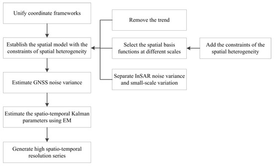
Figure 1.
The flow chart of spatially heterogeneous land surface deformation data fusion method (eSTRE) based on STRE model.
3. Data Sets
3.1. Simulated Data
In order to validate the effectiveness of heterogeneous land surface deformation data fusion method based on STRE model, we simulate the deformation sequence with two local deformation sources. The simulation process is as follows:
(1) Construct the spatial base functions
In the domain , the spatial base functions in bi-square function are established at three different scales. In the first scale, we set homogeneous spatial bases in the whole study area to simulate the whole spatially homogeneous deformation. In the second and third scale, we set heterogeneous spatial bases in two local areas to spatially simulate heterogeneous land surface deformation. The centers for the first, second and third scales are , and , respectively (the asterisk in this sentence indicates multiplication sign).
(2) Construct the initial state quantity
We construct a spatial covariance matrix obeying exponential distribution (, [18]) and take Cholesky decomposition of , e.g., . Then the state quantity represents , .
(3) Generate deformation values for each day
In the random walk model, let , , with . The high spatio-temporal deformation data can be obtained using .
(4) Simulate quasi-real InSAR data
We select 24 real deformation fields from high spatio-temporal resolution deformation data with a time interval of 30 days as the quasi-real InSAR data.
(5) Simulate quasi-real GNSS data
We select 58 sparse GNSS monitoring sites from high spatio-temporal resolution deformation data and take the reserve deformation value in the temporal domain as the quasi-real values for high temporal resolution GNSS data.
(6) Add noise
We add Gaussian white noise with standard deviation of 10 mm to the quasi-real InSAR data and standard deviation of 5 mm to the quasi-real GNSS data.
The simulated GNSS and InSAR data are shown in Figure 2 and Figure 3, respectively. As shown in Figure 2, the influence range of two local deformation sources in the simulated area gradually expanded. The two deformation sources cause different surface deformations: the upper left deformation source causes the ground to sink, and the lower right deformation source causes the ground to rise.
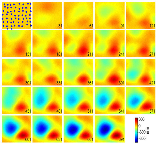
Figure 2.
Simulated InSAR data. The blue points in the first InSAR image are the selected 58 GNSS stations, and the number at the bottom right of each image is the InSAR monitoring day.
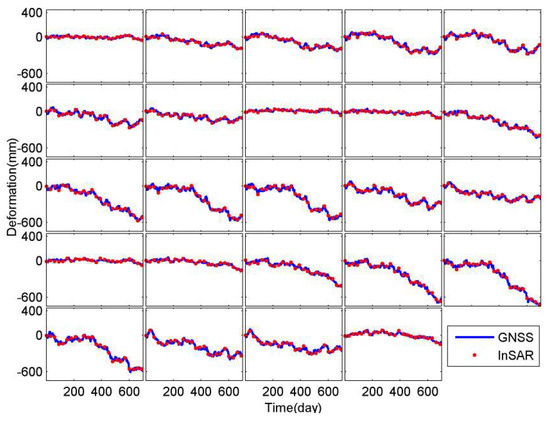
Figure 3.
Simulated GNSS data of 24 random GNSS stations. The blue line is the GNSS time series and the red circles are the closest InSAR pixel time series to the GNSS sites.
The blue line in Figure 3 represents the simulated GNSS time series, and the red circles indicate the closest InSAR pixel time series to the GNSS site. The red circles almost entirely coincide with the blue line, indicating that the simulated GNSS data coincide well with the InSAR data.
3.2. Los Angeles Data
In order to compare the eSTRE and the STRE methods, we use the same real experiment data used by Liu et al. [17]. 15 ENVISAT ASAR descending orbit images covering the whole Los Angeles area from 27 September 2003 to 7 December 2009 were selected, which are processed using the small-baseline subset (SBAS) method based on GAMMA software. GPS time series in this area are downloaded from the SOPAC website (ftp://sopac-ftp.ucsd.edu/pub/timeseries/). The range of InSAR and the selected GPS sites are shown in Figure 4.
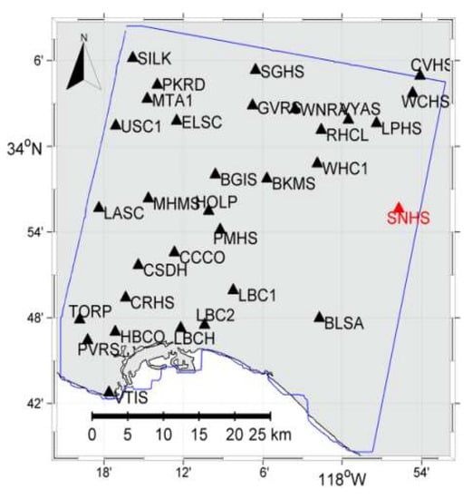
Figure 4.
The range of InSAR and the GPS sites. The blue line represents the range of the InSAR data. Black triangles represent the selected GPS sites and the red triangle represents the reference GPS station (SNHS).
Data Processing
Since the InSAR data processed by GAMMA software are only the relative deformation in the line of sight (LOS) direction and GPS time series from the SOPAC website are absolute 3-dimensional deformation. We convert GPS 3-dimensional results into LOS direction [29] and InSAR data are converted to absolute deformation using the InSAR data closed to SNHS reference station. The InSAR and GPS measurements after using a unifying coordinate framework are shown in Figure 5 and Figure 6.
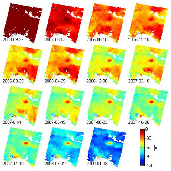
Figure 5.
The InSAR measurements after using a unifying coordinate framework. The number at the bottom left of each figure indicates the monitoring date. This figure is quoted from Figure 14 of Liu et al. [17].
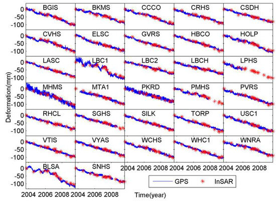
Figure 6.
The GPS measurements after using a unifying coordinate framework. Red asterisks are the closest InSAR time series to GPS sites.
4. Simulation Experiment Results and Analysis
In order to test the validity of the eSTRE model, two methods are used to fuse GNSS data and InSAR data simulated in Section 3.1: (STRE) establish an homogeneous spatial model without taking the spatially heterogeneity into consideration; (eSTRE) establish a unified spatial model with the constraints of local spatial heterogeneity.
The selection of spatial base functions will directly affect the accuracy of the spatial model. Too few spatial base functions cannot capture all the spatial variability. However, too many spatial base functions cost a lot of computer time and are also prone to causing the over-fitting phenomenon. As is shown in Figure 2, the deformation field is always subsidence or uplift and the last InSAR image contains all the deformation information in the monitoring area. Therefore, we select the spatial base functions based on the last InSAR image to capture all the spatial variability. The spatial bases are setting from different scales until the spatial residuals (Equation (6)) fitted by least square are stable. Where is the observed value, is the global spatio-temporal trend, are the chosen rank base functions, and is the transposition operator.
The first modeling method selects the whole spatial base functions based on the above principles and establishes a spatially homogeneous model without the constraints of spatial heterogeneity. For the second modeling method, the local spatial base functions are selected according to the influence range of the local deformation sources to fit the spatially heterogeneous land surface deformation caused by local deformation sources, which are added to the model established in the first modeling method. The second method in Section 2.2 is used to select the local spatial base functions. Firstly, the influence range of the local deformation source is determined based on the last InSAR image (Figure 7). As shown in Figure 7, the upper left deformation source results the ground to sink, and the lower right deformation source results the ground to rise. Therefore, we select the two regions as the heterogeneous surface deformation regions. Secondly, the local spatial base functions are selected based on Equation (6) using bi-square spatial bases (Equation (7), where is the position of the th scale spatial basis, is the th scale spatial variation range.) for the heterogeneous surface deformation regions. We adjust the position and number of spatial bases for each of the two heterogeneous surface deformation regions, to make the spatial residuals (Equation (6)) fitted by least square are stable. This results in bi-square spatial bases with 63 for the upper left regions and 42 for the lower right regions. Center positions for spatial bases are uniformly distributed in the heterogeneous surface deformation regions (Figure 4).
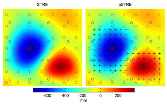
Figure 7.
The distribution of the spatial bases. Blue circles are the first scale spatial bases with the x-to-y interval 110 km. Red circles are the second scale spatial bases with the x-to-y interval 60 km. Black circles are the third scale spatial bases with the x-to-y interval 30 km.
The distribution of the spatial bases selected by the two methods is shown in Figure 7. The left panel in Figure 7 shows the homogeneous spatial bases without the constraints of spatial heterogeneity, and the right panel in Figure 7 shows the heterogeneity spatial bases with the constraints of spatial heterogeneity. The red and blue circles represent the whole spatial bases, and the black “+” represents the local spatial bases.
The residuals of InSAR data fitted by the spatial bases are analyzed to test the validity of both methods. Due to the limited layout, we only select the last phase InSAR residuals (Figure 8) for the analysis in this paper. We can see from Figure 8 that the fitted residuals of eSTRE (RMS = 10.26 mm) are more stable than that of STRE (RMS = 11.71 mm), showing that the spatial model with the constraints of spatial heterogeneity has a better accuracy than that without the constraints of spatial heterogeneity.
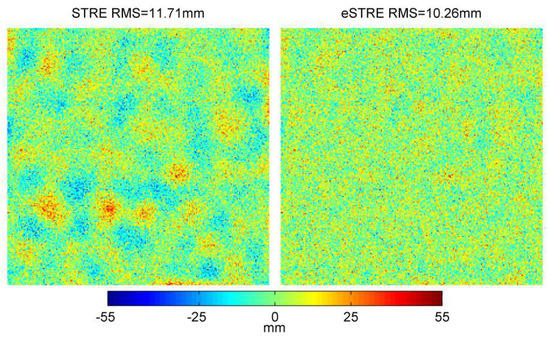
Figure 8.
The residuals of the last InSAR data fitted by the spatial base functions. The left panel represents the residuals fitted by STRE and the right panel represents the residuals fitted by eSTRE.
In order to further test the validity of eSTRE, the residuals between the smoothing values and true values are compared, and the last 12 phases of residuals are shown in Figure 9.
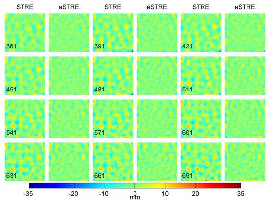
Figure 9.
The last 12 phases residuals of InSAR data for smoothing results. The left panel and right panel of each pair represents the residuals of STRE and eSTRE. The number at the bottom left of each subfigure indicates the monitoring day.
As Figure 9 shows, we can see that the residuals obtained from eSTRE are more stable than those obtained from STRE. In order to quantitatively analyze the advantages of eSTRE, the statistic RMS value of residuals of merged results for last 12 phases InSAR data are calculated in Table 1. As can be seen from Table 1, the accuracy of eSTRE is better than that of STRE, and the average improvement rate is 17.5%.

Table 1.
The RMS values of residuals of smoothing results for the last 12 phases of InSAR data (unit: mm).
In order to comprehensively analyze the effectiveness of eSTRE, we select six GNSS stations within and outside the range of each deformation source for analysis. The selected GNSS stations are shown in Figure 10.
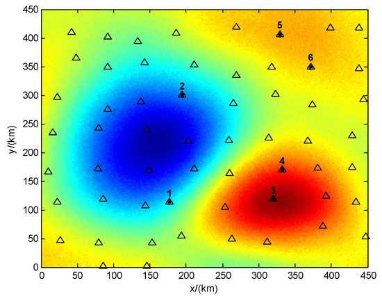
Figure 10.
The locations of the selected GNSS stations marked with asterisk ‘*’ and triangle.
Similar to the analysis of InSAR data, the residuals of smoothing result of the six GNSS stations are drawn in Figure 11. As we can see from Figure 11, the smoothing residuals (the red lines) obtained by eSTRE are more stable than those (the blue lines) obtained by STRE. The RMS statistics of the residuals show that the accuracy of eSTRE is better than that of STRE, and the average improvement rate is 27.4% for the GNSS results. In addition, we also can see from Table 2 that the improvement rates of the GNSS stations (No.1, 2, 3 and 4) in and around the deformation sources are more significant than those far away (No.5 and 6) from the deformation sources, which further confirms the validity of eSTRE.
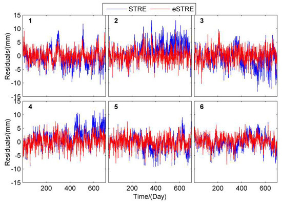
Figure 11.
The residuals of smoothing result of the selected GNSS data. The blue line represents the residuals smoothed by STRE and the red line represents the residuals smoothed by eSTRE.
Table 2.
The RMS values of residuals of smoothing result for the selected GNSS data (unit: mm).
The above analysis indeed confirms that smoothing result of the proposed spatially heterogeneous land surface deformation data fusion method (eSTRE) can provide better accuracy than the previous proposed fusion method (STRE) used by Liu et al. [17]. In order to verify the reliability of the improved fusion method, its interpolation accuracy for missing GNSS data and InSAR data was tested.
To do so, we randomly choose data of 8 days in the temporal domain to evaluate the fusion accuracy in the spatial domain (Figure 12). As is shown in Figure 12, we can visually remark that the residuals obtained by eSTRE are more accurate and stable than those obtained by STRE. In order to quantitatively analyze the effect of improvement, the RMS values of residuals are presented in Table 3. Table 3 shows that the interpolation accuracy of eSTRE for missing InSAR data is better than that of STRE, and the average improvement is 13.6%.
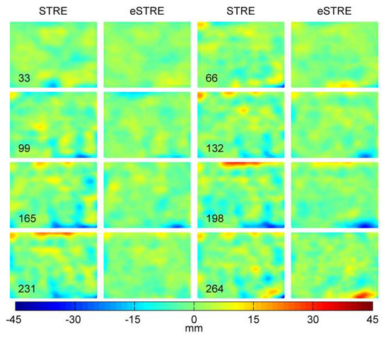
Figure 12.
The residuals of InSAR data in the temporal domain. The left panel and right panel of each pair represents the residuals of STRE and eSTRE. The number at the bottom left of each subfigure indicates the monitoring day.
Table 3.
The RMS values of residuals for the selected InSAR data in the temporal domain (unit: mm).
We also randomly choose 6 points in the spatial domain to evaluate the fusion accuracy in the temporal domain (Figure 13). As is shown in Figure 13, the residuals obtained by eSTRE are more stable than those obtained by STRE for the missing GNSS data. The quantitative analysis of interpolation residuals shows that the interpolation accuracy of eSTRE for missing GNSS data is better than that of STRE, and the average improvement is 51.5%. Figure 13 and Table 4 also show that the improvement effect for the GNSS stations (No.1, 2, 3 and 4) near the deformation sources is better than those stations (No.5 and 6) far away from the deformation sources, indicating that the GNSS stations far away from the deformation sources are less affected by the spatial heterogeneity.
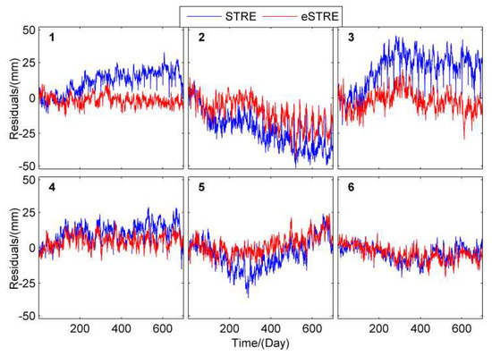
Figure 13.
The residuals of GNSS station data in the spatial domain. The blue line represents the residuals of STRE and the red line represents the residuals of eSTRE.
Table 4.
The RMS values of residuals for the selected GNSS station data in the spatial domain (unit: mm).
In summary, the simulation experiment shows that the fusion method with the constraints of spatial heterogeneity based eSTRE model is more compatible with the heterogeneity surface deformation caused by the multi-deformation source, and the fusion accuracy is higher than that without the constraints of spatial heterogeneity.
5. Los Angeles Experiment Results and Analysis
In Figure 5, we can find that there is a spatially heterogeneous area in the middle of the study area, and the subsidence speed of this area is slower than that in the surrounding area. We infer that there is a difference in geological structure between this area and its surrounding area. In order to eliminate the differences caused by spatial heterogeneity, the spatial bases in the spatially heterogeneous area are established separately. Since we do not know the specific range of the spatially heterogeneous area, we add the local spatial bases of the spatially heterogeneous area based on the last phase InSAR image with the most complicated deformation according to the eSTRE method. The selected spatial bases are shown in Figure 14.
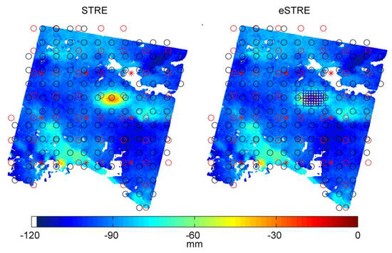
Figure 14.
The selected spatial bases of the whole monitoring area. The left panel represents the selected spatial bases according to the STRE method used in Liu et al. [17], and the right panel represents the selected spatial bases according to the eSTRE method described in Section 2.2. The red and black circles and the red asterisks represent the whole spatial bases, and the blue circles and “+” represents the local spatial bases.
We can see from Figure 14 that we choose 3 layers of spatial bases (the red asterisks ‘*’, the black circles and the red circles) for the STRE method. We add two scales of spatial bases (the blue plus ‘+’ and the blue circles) to the spatially heterogeneous area for eSTRE. Since the range of the spatially heterogeneous area is too small, the spatially heterogeneous area is extracted for analysis, which is shown in Figure 15. As can be seen in the left panel of Figure 15, the number of spatial bases selected by STRE in the spatially heterogeneous area is small, while that selected by eSTRE are uniformly distributed in the spatially heterogeneous area, which can better capture the local variation in the spatially heterogeneous area.
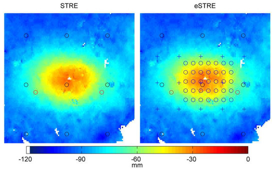
Figure 15.
Zoom-in of Figure 14 for the selected spatial bases in the spatially heterogeneous area. The left panel represents the selected spatial bases in the spatially heterogeneous area according to the STRE method and the right panel represents the selected spatial bases in the spatially heterogeneous area according to the eSTRE method.
Similar to the simulated experiment, the smoothing results and the cross-validation results of InSAR and GPS are analyzed. Since the range of the spatially heterogeneous area is small, the influence range of the spatially heterogeneous area is also small, meaning there is only a slight difference in smoothing residuals of InSAR data for both methods, which cannot be discerned visually from the residual graph. Therefore, the smoothing residuals graphs for both methods are not shown here, and only the statistics of the residuals (Table 5) are analyzed. In Table 5, we see that eSTRE has better modeling accuracy for the whole monitoring area and the local spatially heterogeneous area than that in STRE. The average improvement rate of the entire monitoring area is 11.4%, while that of the local spatially heterogeneous area is 33.3%.
Table 5.
The RMS statistics of InSAR data for both methods (unit: mm).
In order to analyze the improvement of eSTRE for the smoothing results, three GPS monitoring stations (one station (BKMS) is close to the spatially heterogeneous area, and the other two stations (MHMS and LBCH) are away from the spatially heterogeneous area) are selected for detailed analysis. The selected three GPS stations are shown in Figure 16 and their smoothing (misfit reduction) results are shown in Figure 17. As can be seen from Figure 17, the two modeling methods have better smoothing accuracy for GPS data, and the smoothing precision of eSTRE is slightly better than that of STRE.
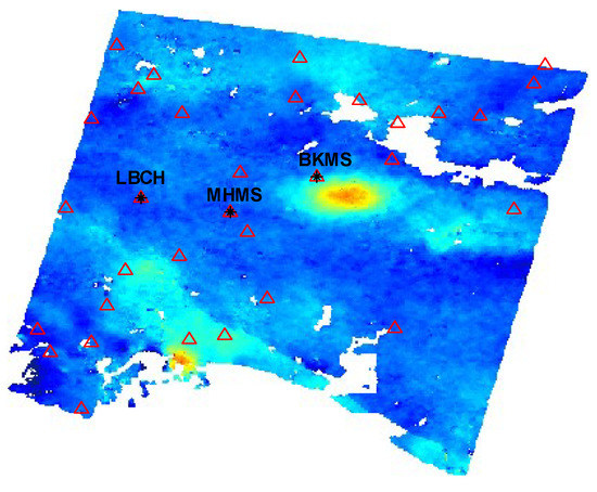
Figure 16.
The locations of the selected GPS stations marked with asterisk ‘*’.
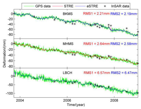
Figure 17.
Smoothing results of the selected GPS data. Green lines are the source GPS time series, blue lines are the smoothing results obtained by STRE, red lines are the smoothing results obtained by eSTRE and black asterisks are time series of the InSAR pixel closest to GPS site.
The above analysis verifies the modeling method with the constraints of spatial heterogeneity can improve the smoothing accuracy of InSAR data and GPS data. In order to further verify the effectiveness of the method, we use cross-validation method to compare the interpolation accuracy for missing InSAR data and GPS data. The cross-validation residuals of InSAR data are shown in Figure 18 and Figure 19. We can see from Figure 18 and Figure 19 that similar to the smoothing results of the simulated experiment, the cross-validation accuracy of eSTRE for the whole monitoring area is a slightly better than that of STRE, while that of eSTRE for the spatially heterogeneous area is significantly better than that of STRE. The RMS statistics of the cross-validation residuals for InSAR data (Table 6) show that the average improvement rate of the whole monitoring area is 6.0%, while that of the local spatially heterogeneous area is 22.6%.
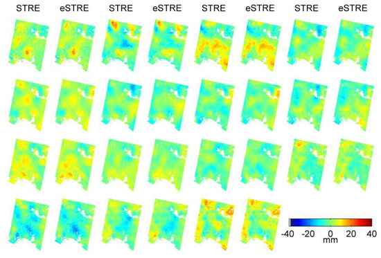
Figure 18.
The cross-validation residuals of InSAR data for the whole monitoring area, sampled on the dates given in Table 6. The left panel and right panel of each pair represents the residuals of STRE and eSTRE.
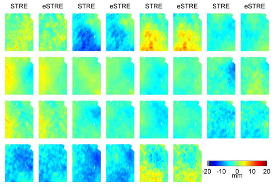
Figure 19.
The cross-validation residuals of InSAR data for the local heterogeneous area, sampled on the dates given in Table 6. The left panel and right panel of each pair represents the residuals of STRE and eSTRE.
Table 6.
The cross-validation residuals statistics of InSAR data for both methods (unit: mm).
Through the cross-validation experiment, it is proved that the spatially heterogeneous land surface deformation data fusion method (eSTRE) can effectively improve the interpolation accuracy of the missing InSAR data.
We further use cross-validation method to test the effect of eSTRE on missing GPS data, and the selected three GPS stations are shown in Figure 16. The interpolation results of GPS data by both methods are shown in Figure 20. In Figure 20, we can see that the results obtained by eSTRE are more stable than those obtained by STRE for the GPS station (BKMS) which is close to the spatially heterogeneous area with an average improvement of 14.4%, while the GPS interpolation results obtained by both methods are similar for GPS stations far away from the spatially heterogeneous area (MHMS and LBCH), and their RMS values are almost equal. The cross-validation experiments of GPS data further confirm that the eSTRE method with the constraints of spatial heterogeneity can achieve better fusion accuracy.
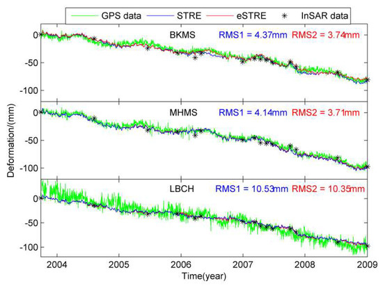
Figure 20.
The cross-validation results of the selected GPS data for both methods. Green lines are the source GPS time series, blue lines are the interpolation results obtained by STRE, red lines are the interpolation results obtained by eSTRE and black asterisks are time series of the InSAR pixel closest to GPS site.
6. Discussion
Fusing InSAR and GNSS measurements to obtain high spatio-temporal resolution data is a research hotspot in land surface deformation. Existing fusion methods usually use the DIDP approach without sufficiently considering certain complicated temporal and spatial characteristics of the surface deformation. The dynamic filtering fusion model proposed by Liu et al. [17] ignores that weakness and is only able to obtain high precision fusion results for the homogeneous surface deformation. However, their method does not consider the spatial heterogeneity and is not appropriate for the heterogeneous surface deformation. In this study, we integrate the spatial heterogeneous constraints into a spatio-temporal Kalman model to improve the fusion precision. The experiment results show that the better accuracies are achieved for eSTRE than for the previous STRE fusion model.
As a future outlook, the eSTRE method presented in this paper can be applied to generate high spatio-temporal resolution data for heterogeneous land surface deformation, e.g., the land surface deformation caused by coal mining, groundwater exploitation, oil exploitation and so on. The high spatio-temporal resolution data obtained by eSTRE can help us to better understand the mechanism of heterogeneous land surface deformation, and then, we can use the method to establish spatio-temporal forecasting models for geological disasters or invert parameters of subsidence for heterogeneous land surface deformation, such as coal mining, groundwater exploitation, oil exploitation and so on.
However, both STRE and eSTRE method have a strong dependence on the selection of the spatial bases. Moreover, the spatial bases selected in this paper need to be refined in order to find the better ones based on some experience. Few spatial base functions cannot capture all the spatial variability. However, too many spatial base functions cost a lot of computer time and are also prone to causing the over-fitting phenomenon. Moreover, if the deformation field or a sub field is progressing from even to subsidence then to uplift then to even, the method of selecting spatial base used in this paper will fail. Therefore, developing a method that can select the optimal spatial bases adaptively will be our future research work. Otherwise, the eSTRE method proposed in this paper was tested only using ENVISAT ASAR data, meaning more InSAR data and deformation data should be used to test the improved performance of eSTRE.
7. Conclusions
For monitoring spatially heterogeneous land surface deformation, this paper proposes an enhanced fusion method with the constraints of spatial heterogeneity based on an STRE model called eSTRE. This new method takes into account the impact of spatially heterogeneous sources on the deformation results by establishing the extra spatial bases for the spatially heterogeneous area. When the range of the spatially heterogeneous deformation sources is known, we can construct corresponding spatial bases within the influence of spatially heterogeneous deformation sources. When the distribution range of spatially heterogeneous deformation sources is unknown, we can set spatial bases according to the InSAR images containing the most complicated deformation. In this paper, simulation experiments and real experiments in Los Angeles area prove that the new eSTRE model with the constraints of spatial heterogeneity can consider the spatial heterogeneity in different areas, and the results show that the eSTRE method can reduce the root mean square (RMS) of InSAR interpolation results by 14% and 23% on average for a simulation experiment and Los Angeles experiment, respectively, indicating that the new proposed method (eSTRE) is substantially better than the previous STRE fusion model and that the eSTRE method can provide more invaluable information for space geodesy, especially in regards to heterogeneous land surface deformation monitoring.
Author Contributions
Q.S. and W.D. conceived and designed the experiments; R.S. and Z.L. polish the paper and gave constructive advice; N.L. contributed to the discussion of the results.
Funding
This work was supported by the National Natural Science Foundation of China under Grant 41674011, Innovation Foundation for Postgraduate of Central South University, China (No. 2018zzts033), and Innovation Foundation for Postgraduate of Hunan Province, China (No. CX2018B104).
Acknowledgments
The ENVISAT Interferometric Synthetic Aperture Radar data were supplied by the European Space Agency and Global Positioning System data were downloaded from the Scripps Orbit and Permanent Array Center website.
Conflicts of Interest
The authors declare no conflict of interest.
References
- Lanari, R.; Mora, O.; Manunta, M.; Mallorquí, J.J.; Berardino, P.; Sansosti, E. A small-baseline approach for investigating deformations on full-resolution differential SAR interferograms. IEEE Trans. Geosci. Remote Sens. 2004, 42, 1377–1386. [Google Scholar] [CrossRef]
- Jo, M.J.; Jung, H.S.; Won, J.S.; Lundgren, P. Measurement of three-dimensional surface deformation by Cosmo-SkyMed X-band radar interferometry: Application to the March 2011 Kamoamoa fissure eruption, Kīlauea Volcano, Hawai’i. Remote Sens. Environ. 2015, 169, 176–191. [Google Scholar] [CrossRef]
- Zhao, R.; Li, Z.W.; Feng, G.C.; Wang, Q.J.; Hu, J. Monitoring surface deformation over permafrost with an improved SBAS-InSAR algorithm: With emphasis on climatic factors modeling. Remote Sens. Environ. 2016, 184, 276–287. [Google Scholar] [CrossRef]
- Chaussard, E.; Wdowinski, S.; Cabral-Cano, E.; Amelung, F. Land subsidence in central Mexico detected by ALOS InSAR time-series. Remote Sens. Environ. 2014, 140, 94–106. [Google Scholar] [CrossRef]
- Simonetto, E.; Durand, S.; Burdack, J.; Polidori, L.; Morel, L.; Nicolas-Duroy, J. Combination of INSAR and GNSS measurements for ground displacement monitoring. Procedia Technol. 2014, 16, 192–198. [Google Scholar] [CrossRef][Green Version]
- Fukushima, Y. Correction of DInSAR noise using GNSS measurements. In Proceedings of the 2013 Asia-Pacific Conference on Synthetic Aperture Radar (APSAR), Tsukuba, Japan, 23–27 September 2013; pp. 226–228. [Google Scholar]
- Hoeven, A.; Hanssen, R.; Ambrosius, B. Cross-Validation oftropospheric delay variability observed by GPS and SAR interferometry. GPS Nieuwsbr. 2000, 2, 2–7. [Google Scholar]
- Li, Z.W.; Ding, X.L.; Liu, G.X. Modeling atmospheric effects on InSAR with meteorological and continuous GPS observations: Algorithms and some test results. J. Atmos. Sol.-Terr. Phys. 2004, 66, 907–917. [Google Scholar] [CrossRef]
- Li, Z.; Fielding, E.J.; Cross, P. Separating slow deformation signals from water vapour and orbital errors using a single InSAR interferogram. In Proceedings of the American Geophysical Union, Fall Meeting 2006, San Francisco, CA, USA, 7–11 December 2009. Abstract G22A-05. [Google Scholar]
- Samsonov, S.; Tiampo, K. Analytical Optimization of a DInSAR and GPS Dataset for Derivation of Three-Dimensional Surface Motion. IEEE. Geosci. Remote Sens. 2006, 3, 107–111. [Google Scholar] [CrossRef]
- Samsonov, S.; Tiampo, K.; Rundle, J. Application of DInSAR-GPS Optimization for Derivation of Fine-Scale Surface Motion Maps of Southern California. IEEE Trans. Geosci. Remote Sens. 2007, 45, 512–521. [Google Scholar] [CrossRef]
- Komac, M.; Holley, R.; Mahapatra, P.; van der Marel, H.; Bavec, M. Coupling of GPS/GNSS and radar interferometric data for a 3D surface displacement monitoring of landslides. Landslides 2015, 12, 241–257. [Google Scholar] [CrossRef]
- Farolfi, G.; Bianchini, S.; Casagli, N. Integration of GNSS and Satellite InSAR Data: Derivation of Fine-Scale Vertical Surface Motion Maps of Po Plain, Northern Apennines, and Southern Alps, Italy. IEEE Trans. Geosci. Remote Sens. 2019, 57, 319–328. [Google Scholar] [CrossRef]
- Ge, L.; Han, S.; Rizos, C. Interpolation of GPS results incorporating geophysical and InSAR information. Earth Planets Space 2000, 52, 999–1002. [Google Scholar] [CrossRef]
- Ge, L.; Han, S.; Rizos, C. The Double Interpolation And Double Prediction (didp) Approach For Insar And Gps Integration. In Proceedings of the 19th International. Society of Photogrammetry & Remote Sensing Congress & Exhibition, Amsterdam, The Netherlands, 16–23 July 2000; pp. 205–212. [Google Scholar]
- Xu, C. Prospect on the Integration of GPS and INSAR Data. Geomat. Inf. Sci. Wuhan Univ. 2003, 28, 58–61. [Google Scholar]
- Liu, N.; Dai, W.; Santerre, R.; Hu, J.; Shi, Q.; Yang, C. High Spatio-Temporal Resolution Deformation Time Series With the Fusion of InSAR and GNSS Data Using Spatio-Temporal Random Effect Model. IEEE Trans. Geosci. Remote Sens. 2019, 57, 364–380. [Google Scholar] [CrossRef]
- Cressie, N.; Shi, T.; Kang, E.L. Fixed Rank Filtering for Spatio-Temporal Data. J. Comput. Graph. Stat. 2010, 19, 724–745. [Google Scholar] [CrossRef]
- Kang, E.L.; Cressie, N.; Shi, T. Using temporal variability to improve spatial mapping with application to satellite data. Can. J. Stat. 2010, 38, 271–289. [Google Scholar] [CrossRef]
- Hai, N.; Katzfuss, M.; Cressie, N.; Braverman, A. Spatio-Temporal Data Fusion for Very Large Remote Sensing Datasets. Technometrics 2014, 56, 174–185. [Google Scholar]
- Nguyen, H.; Cressie, N.; Braverman, A. Multivariate Spatial Data Fusion for Very Large Remote Sensing Datasets. Remote Sens. 2017, 9, 142. [Google Scholar] [CrossRef]
- Cressie, N.; Johannesson, G. Fixed rank kriging for very large spatial data sets. J. R. Stat. Soc. Ser. B Stat. Methodol. 2008, 70, 209–226. [Google Scholar] [CrossRef]
- Vidakovic, B. Statistical Modeling by Wavelets; Wiley: Hoboken, NJ, USA, 1999; pp. 316–317. [Google Scholar]
- Wahba, G. Spline models for observational data. In Proceedings of the Cbms-Nsf Regional Conference, Columbus, OH, USA, 23–27 March 1987; Series in Applied Mathematics, Based on A Series of 10 Lectures at Ohio State University at Columbus. Society for Industrial and Applied Mathematics: Philadelphia, PA, USA, 1990; pp. 113–114. [Google Scholar]
- Trevor, H.; Tibshirani, R.; Friedman, J. The Elements of Statistical Learning: Data mining, Inference and Prediction; Springer: New York, NY, USA, 2001; p. 13. [Google Scholar]
- Katzfuss, M.; Cressie, N. Spatio-temporal smoothing and EM estimation for massive remote-sensing data sets. J. Time Ser. Anal. 2011, 32, 430–446. [Google Scholar] [CrossRef]
- Hu, J.; Li, Z.W.; Sun, Q.; Zhu, J.J.; Ding, X.L. Three-Dimensional surface displacements from insar and gps measurements with variance component estimation. IEEE Geosci. Remote Sens. Lett. 2012, 9, 754–758. [Google Scholar]
- Neal, R.M.; Hinton, G.E. A View of the Em Algorithm that Justifies Incremental, Sparse, and other Variants. In Learning in Graphical Models; Jordan, M.I., Ed.; Springer: Dordrecht, The Netherlands, 1998; pp. 355–368. [Google Scholar]
- Fialko, Y.; Simons, M.; Agnew, D. The complete (3-D) surface displacement field in the epicentral area of the 1999 M W 7.1 Hector Mine Earthquake, California, from space geodetic observations. Geophys. Res. Lett. 2001, 28, 3063–3066. [Google Scholar] [CrossRef]
© 2019 by the authors. Licensee MDPI, Basel, Switzerland. This article is an open access article distributed under the terms and conditions of the Creative Commons Attribution (CC BY) license (http://creativecommons.org/licenses/by/4.0/).