Article

GNSS/INS/LiDAR-SLAM Integrated Navigation System Based on Graph Optimization

GNSS Research Center, Wuhan University, 129 Luoyu Road, Wuhan 430079, China
*
Author to whom correspondence should be addressed.
Remote Sens. 2019, 11(9), 1009; https://doi.org/10.3390/rs11091009
Submission received: 3 April 2019 / Revised: 19 April 2019 / Accepted: 23 April 2019 / Published: 28 April 2019

Abstract

:
A Global Navigation Satellite System (GNSS)/Inertial Navigation System (INS)/Light Detection and Ranging (LiDAR)-Simultaneous Localization and Mapping (SLAM) integrated navigation system based on graph optimization is proposed and implemented in this paper. The navigation results are obtained by the information fusion of the GNSS position, Inertial Measurement Unit (IMU) preintegration result and the relative pose from the 3D probability map matching with graph optimizing. The sliding window method was adopted to ensure that the computational load of the graph optimization does not increase with time. Land vehicle tests were conducted, and the results show that the proposed GNSS/INS/LiDAR-SLAM integrated navigation system can effectively improve the navigation positioning accuracy compared to GNSS/INS and other current GNSS/INS/LiDAR methods. During the simulation of one-minute periods of GNSS outages, compared to the GNSS/INS integrated navigation system, the root mean square (RMS) of the position errors in the North and East directions of the proposed navigation system are reduced by approximately 82.2% and 79.6%, respectively, and the position error in the vertical direction and attitude errors are equivalent. Compared to the benchmark method of GNSS/INS/LiDAR-Google Cartographer, the RMS of the position errors in the North, East and vertical directions decrease by approximately 66.2%, 63.1% and 75.1%, respectively, and the RMS of the roll, pitch and yaw errors are reduced by approximately 89.5%, 92.9% and 88.5%, respectively. Furthermore, the relative position error during the GNSS outage periods is reduced to 0.26% of the travel distance for the proposed method. Therefore, the GNSS/INS/LiDAR-SLAM integrated navigation system proposed in this paper can effectively fuse the information of GNSS, IMU and LiDAR and can significantly mitigate the navigation error, especially for cases of GNSS signal attenuation or interruption.

1. Introduction

With the rapid development of autonomous driving and intelligent robots, the demand for navigation information with high data rates, high precision and all-weather features continues to increase, especially in complex urban environments. Thus, a single navigation technique can hardly meet the requirements for practical applications, and the synthesis of multiple navigation techniques has become the development trend in navigation. Among the various synthesized navigation techniques, the Global Navigation Satellite System/Inertial Navigation System (GNSS/INS) integrated navigation system, which is dominated by the INS and supplemented by the GNSS, is the most popular. The characteristics of the GNSS and the INS are distinctively complementary: (1) generally, information from GNSS and INS are effectively integrated via Kalman filtering [1]; and (2) INS largely compensates for the shortcoming of GNSS, which is vulnerable to interference, while GNSS provides the periodic correction information for INS; hence, the synergy of the two techniques improves the navigation performance. However, in areas where the GNSS signal is not available, the GNSS/INS integrated navigation system relies on the performance of INS alone and experiences drifting errors. In addition, for the low-cost MEMS (Micro-Electro-Mechanical System)-Inertial Measurement Unit (IMU), the navigation errors will accumulate and increase rapidly over time. In the context of low-cost integrated systems, image-based methodologies have also been explored, aiming at investigating the impact of drifts and errors experienced with such techniques, like in [2,3]. In the field of computer vision and robotics, Simultaneous Localization and Mapping (SLAM) technology is widely used for navigation in unfamiliar environments. The SLAM system locates itself mainly according to position estimation and a map during movement and builds up incremental maps based on the self-localization to achieve independent positioning and navigation [4]. In recent years many excellent SLAM systems based on a single sensor have been developed, such as LG-SLAM [5], IMLS-SLAM [6], SUMA [7] and LOAM [8]. VINS [9] uses a tightly coupled, nonlinear optimization-based method to obtain highly accurate visual-inertial odometry by fusing preintegrated IMU measurements and feature observations. vLOAM [10] presents a general framework for combining camera and Light Detection and Ranging (LiDAR). However, the errors of these SLAM systems, which are reduced mainly by the closed-loop correction method, will also increase with the moving distance. In large-scale outdoor motion, SLAM is less likely to form a closed-loop. Additionally, SLAM cannot provide absolute navigation information. Therefore, the combination of the GNSS/INS integrated navigation system and SLAM will effectively mitigate the navigation drift when the GNSS signal is not available, reduce the dependence of SLAM on closed-loop correction and provide absolute navigation information to fulfill the complementary advantages of the three techniques.
Generally, cameras and LiDAR are the two most common sensors for SLAM, and each of the two types of sensors has strengths and weaknesses. Compared to the camera, LiDAR, despite a higher cost and lower resolution, can directly obtain the structure information of environments and is hardly influenced by light or weather. Therefore, in this paper, mechanical rotating LiDAR is adopted.
In order to estimate pose change from LiDAR measurements, there are about three different categories of scan matching method: feature-based scan matching, point-based scan matching and mathematical property-based scan matching [11]. The feature-based scan matching is matching with some key elements which can be geometric primitives such as points, lines, and polygons, or a combination thereof in the LiDAR data. The point-based scan matching directly searches and matches the corresponding points in the LiDAR data. The Iterative Closest Point (ICP) algorithm and its variants [12,13] are the most popular methods to solve the point-based scan matching problem. The mathematical property-based scan matching can use various mathematical properties, such as the Normal Distribution Transform (NDT) [14] or the probability grid [15] to depict scan data changes. The feature-based scan matching method is efficient and accurate. But, it relies on features extracted from the environment. It may fail to work properly in outdoor or indoor unconstructed environments. The point-based scan matching method is accurate and independent of environment features. But, it takes a long time because of the inevitable iteration [16]. Thereby in this paper, the probability grid scan matching is used for the point cloud matching in the outdoor environment.
For data fusion in SLAM, there are mainly two methods: filtering and graph optimization. The former is better than the latter in terms of calculation speed but inferior in accuracy [17]. Qian [18] and Gao [16] used the EKF (extended Kalman filter) to perform a combination of GNSS, INS and LiDAR-SLAM. Shamsudin [19] used particle filtering to combine GNSS with LiDAR-SLAM. There has been increasing research on graph optimization in recent years. Kukko [20] used the graph optimization method to combine the results of the GNSS/INS with a single-line LiDAR. Hess [15] implemented 2D-LiDAR navigation based on graph optimization. Pierzchała [21] used graph optimized 3D LiDAR-SLAM for woods construction. Cartographer [22] completed a fusion of GNSS, 3D-LiDAR and IMU based on graph optimization. However, it was assumed that the vehicle was moving at a low speed and moved smoothly. Therefore, gravity is used to solve the horizontal attitude (i.e., roll and pitch), and error modelling for the IMU bias was ignored; the estimation of the vehicle’s velocity was also ignored.
Considering the limitations of Cartographer and based on the Cartographer codes, a GNSS/INS/LiDAR-SLAM integrated navigation system is implemented in this paper based on graph optimization. First, the MEMS-IMU mechanization is applied to predict the motion of the vehicle and provide the searching initial value for probability map scan matching with LiDAR in the front-end. In the back-end, the GNSS position provides the absolute position constraint, while the IMU preintegration [9,23] is applied to increase the motion constraints, and the LiDAR-SLAM scan matching provides the relative pose constraints. Then, three information sources are combined by graph optimization to obtain the final navigation positioning results. In addition, to keep the parameters of the graph optimization invariant with time, a sliding window is applied to ensure the relative stability of the graph optimization parameter number.
The remainder of the paper is organized as follows. In Section 2, the mathematical model of the GNSS/INS/LiDAR-SLAM integrated navigation system is described. In Section 3, the land vehicle tests are introduced. The experimental results are discussed in Section 4. Finally, in Section 5, conclusions and future prospects are presented.

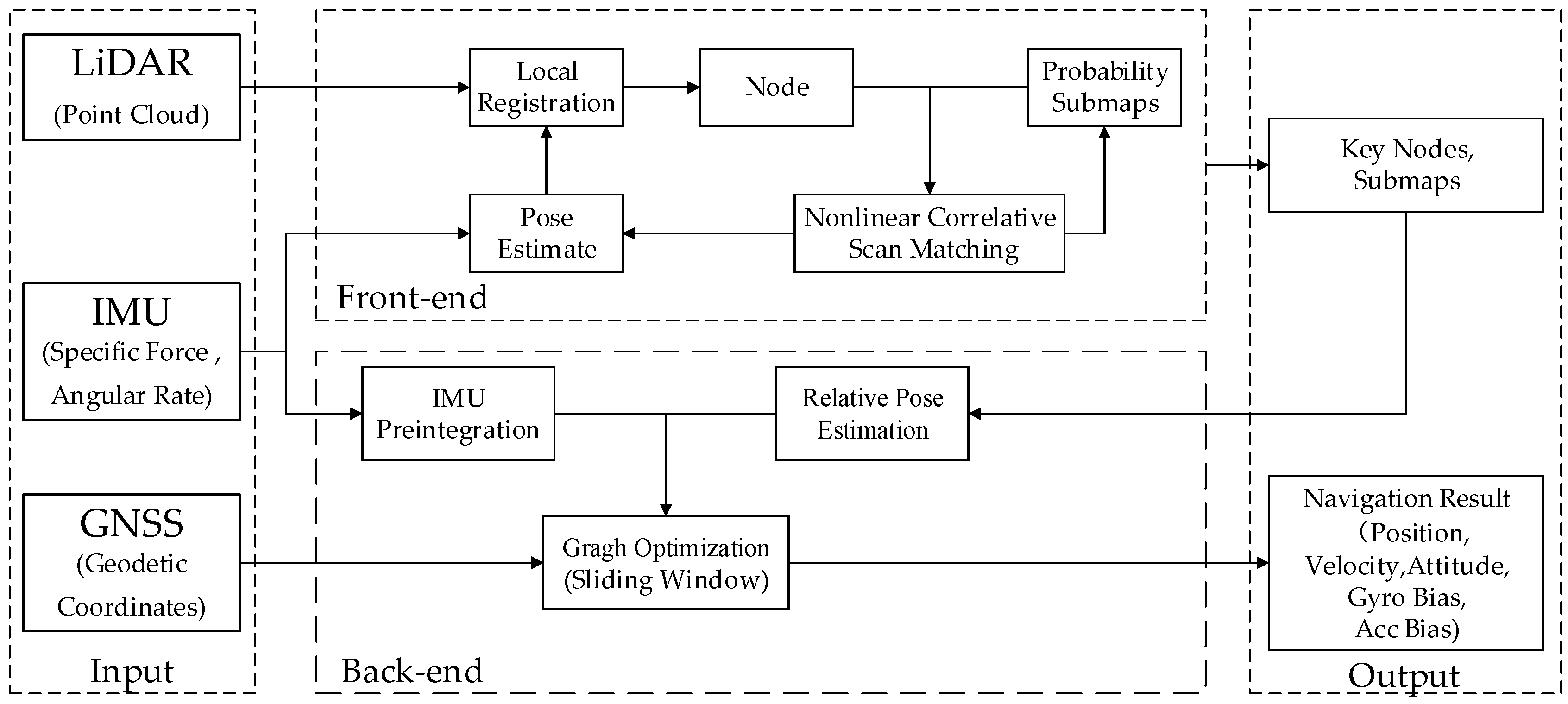
2. GNSS/INS/LiDAR-SLAM Integrated Navigation System

The GNSS/INS/LiDAR-SLAM integrated navigation system, an overview of which is shown in Figure 1, mainly is comprised of two parts: scan matching in the front-end and graph optimization in the back-end. In the front-end scan matching process, the point cloud acquired by LiDAR is first filtered by a voxel filter. Then, with the MEMS-IMU mechanization result, a node is formed, and the initial search value appears. Subsequently, probabilistic map scan matching is conducted for the node, and the node coordinate is obtained in the local coordinate system. Then, the node that meets certain conditions is selected to be inserted into the probability submap, and finally, the probability submap is updated. In the back-end graph optimization process, the cost functions are constructed with the GNSS position observation, the result of the IMU preintegration between two adjacent nodes and the relative pose constraints between the nodes and submaps. A sliding window is applied to ensure the relative stability of the number of optimized variables.

2.1. Coordinate Frame

The GNSS/INS/LiDAR-SLAM integrated navigation system involves multiple coordinate systems, and information fusion in different coordinate systems is needed. The coordinate systems and transformation formula used in the GNSS/INS/LiDAR-SLAM integrated navigation system are given below.

2.1.1. Coordinate System

1. Inertial Coordinate System (i-frame)
The inertial coordinate system is a coordinate system that is invariant in space. The Earth’s inertial coordinate system is usually used to study the motion of the vehicles near the Earth’s surface.
2. Earth-Centered Earth-Fixed Coordinate System (e-frame)
The Earth-centered Earth-fixed coordinate system rotates with the Earth, taking the Earth’s centroid as the coordinate origin, and the X axis points to the intersection of the equator and the prime meridian. The Earth’s rotation axis is taken as the Z axis, and the North Pole is the positive direction. Then, the Y axis is perpendicular to the X-Z plane, forming a right-handed coordinate system.
3. World Coordinate System (w-frame)
The world coordinate system is used to express the GNSS positioning results. The origin is the initial GNSS position, the X-Y plane is the local horizontal plane, with the X axis being the tangential line of the latitude line that points east, and the Y axis is the tangential line of the longitude line that points North. The Z axis is perpendicular to the X-Y plane, forming a right-handed coordinate system.
4. IMU Coordinate System (b-frame)
The IMU coordinate system moves with the vehicle, with the IMU barycenter as the coordinate origin, the X axis points to the right along the IMU horizontal axis, the Y axis points forward along the IMU longitudinal axis, and the Z axis is perpendicular to the X-Y plane, forming a right-handed coordinate system.
5. LiDAR Coordinate System (l-frame)
The LiDAR coordinate system moves with the vehicle, with the LiDAR measurement center as the coordinate origin, the X axis pointing to the right along the LiDAR horizontal axis, the Y axis pointing forward along the LiDAR longitudinal axis, and the Z axis being perpendicular to the X-Y plane, forming a right-handed coordinate system.
6. Map Coordinate System (m-frame)
The map coordinate system is used by LiDAR-SLAM. In this frame, the origin is located where the SLAM is initialized, the X-Y plane is the local horizontal plane, the direction of the X axis is indeterminate, and the yaw between the b-frame and m-frame is 0° on initialization.

2.1.2. Transformation Among Coordinate Systems

All the coordinate transformations in this paper are rigid body transformations. The rigid body transformation from the a-frame to b-frame is defined as follows:
R a b = ( p a b , q a b )
where p a b and q a b are the translation and quaternion from the a-frame to b-frame, respectively.
The rigid body transformation operation is defined as follows:
R b a = ( R a b ) 1 = ( ( C a b ) T p a b , ( q a b ) 1 ) v b = R a b v a = C a b v a + p a b R c a = R b a R c b = ( C b a p c b + p b a , q b a q c b )
where C a b is the direction cosine matrix of q a b and v a is a vector in the a-frame.

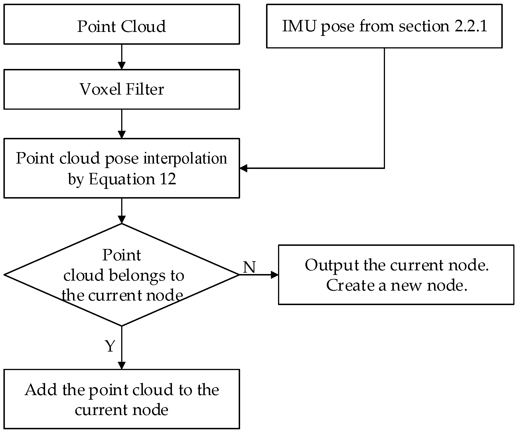
2.2. Front-End Scan Matching

2.2.1. Pose Estimate

In the m-frame, the pose estimate starts from the origin, and the initial yaw between the b-frame and m-frame is set to 0°. The roll and pitch are initialized by gravity when the vehicle is at rest at the beginning. Then, the velocity, position and attitude are updated by the following MEMS-IMU mechanization.
1. Velocity Update
The IMU measures the angular rate ω ˜ i b b between the b-frame and i-frame and the specific force f ˜ b . The velocity differential equation of the strapdown inertial navigation in the e-frame can be obtained by the Coriolis’s theorem [24]:
v ˙ e = C b e f b + g e 2 ω i e e × v e
where v e is the velocity in the e-frame; C b e is the direction cosine matrix of the attitude from the b-frame to the e-frame; g e is gravity in the e-frame; and ω i e e is the angular rate between the e-frame and the i-frame.
The algorithm in this paper aims at the low-cost MEMS-IMU, which has a gyro bias stability that is relatively large (10°/h in this paper) and is incapable of sensing the Earth’s rotation (15°/h). Therefore, the Earth’s rotation can be ignored, i.e., assuming ω i e e = 0 , and Equation (4) is projected to the m-frame as follows:
v ˙ m = C b m f b + g m
After the integral of Equation (4), the velocity update equation is obtained:
v b ( t k ) m = v b ( t k 1 ) m + t k 1 t k [ C b m ( t ) f b ( t ) ] d t + t k 1 t k g m d t
where v b ( t k ) m is the velocity of the IMU in the m-frame at t k .
For vehicles travelling at medium or low speeds (less than 100 m/s), the angular rate and specific force can be assumed to be constant during the IMU sampling interval; that is, according to the single sampling hypothesis [25], the discrete form of Equation (5) is as follows:
v b ( t k ) m = v b ( t k 1 ) m + C b ( t k 1 ) m Δ v b ( t k ) b ( t k 1 ) + g m Δ t k Δ v b ( t k ) b ( t k 1 ) = Δ v f , t k b + 1 2 Δ θ t k × Δ v f , t k b
where Δ v f , t k b and Δ θ t k are the IMU outputs in incremental form with a bias compensation from t k 1 to t k .
Δ v f , t k b = t k 1 t k [ f ˜ b ( t ) b a ( t ) ] d t Δ θ t k = t k 1 t k [ ω ˜ i b b ( t ) b g ( t ) ] d t
where b a and b g are the biases of the accelerometer and gyroscope, respectively.
2. Position Update
The position differential equation in the m-frame is as follows:
p ˙ m = v m
The velocity at t k has been updated, so the position update can be accomplished with the average velocity:
p b ( t k ) m = p b ( t k 1 ) m + v b ( t k 1 ) m Δ t k + 1 2 g m Δ t k 2 + 1 2 C b ( t k 1 ) m Δ v b ( t k ) b ( t k 1 ) Δ t k
where p b ( t k ) m is the position of the IMU in the m-frame at t k .
3. Attitude Update
The attitude is updated by the quaternion as follows [24]:
q b ( t k ) m = q b ( t k 1 ) m q b ( t k ) b ( t k 1 ) q b ( t k ) b ( t k 1 ) = [ cos 0.5 Φ t k sin 0.5 Φ t k Φ t k Φ t k ]
where q b ( t k ) m is the quaternion from the b-frame to the m-frame at t k ; and Φ t k is the equivalent rotation vector of the b-frame from t k 1 to t k . According to the single sampling hypothesis [25], we have the following equation:
Φ t k Δ θ t k

2.2.2. Local Registration

The LiDAR (VLP-16) used in this paper is a mechanical rotary system with a sampling rate of 300–1200 RPM (revolutions per minute). The interval of the two adjacent data packages is approximately 1.3 ms, and one circle of the point cloud contains approximately 154–38 packages. A point cloud circle is used in the scan matching. Therefore, the point cloud data packages need to be spliced to form a circle of point clouds based on the sampling time of a certain package.
Because the amount of point cloud data is relatively large, which affects the speed of point cloud splicing and scan matching, the voxel filter [26] is needed for point cloud downsampling.
Considering the vehicle motion during point cloud collection, motion compensation is required during splicing: here linear interpolation is used, given the factor f = t n t k 1 t k t k 1 ( t k 1 t n t k ) , ω = arccos ( q b ( t k 1 ) m q b ( t k ) m ) , then the position and attitude in the m-frame of the data package at t n is interpolated according to Equation (12) [27] with the position and attitude of the IMU in the m-frame that was obtained in Section 2.2.1. Then, a start time for splicing is selected, and the position and attitude of the data packages within one rotation range are transformed into the relative position and attitude to the start time, as well as the corresponding point cloud. Finally, one circle of the point cloud with the motion compensation, which is recorded as a node, is obtained. The flow of the local registration is shown in Figure 2.
R b ( t n ) m = ( p b ( t k 1 ) m + ( p b ( t k ) m p b ( t k 1 ) m ) f , sin ( 1 f ) ω sin ω q b ( t k 1 ) m + sin f ω sin ω q b ( t k ) m ) R l ( t n ) m = R b ( t n ) m R l b

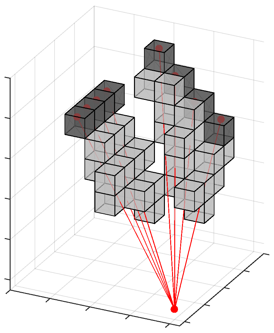
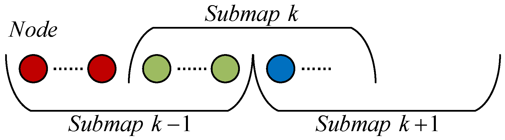
2.2.3. Probability Map

When the scan point is added to the probability map, the scan point is converted into a grid point (such as the dark grey square in Figure 3), which has a probability value that is set as p h i t . The points on the line that connect the scan point and the scan origin, which has a probability value that is set as p m i s s , are also converted into grid points (such as the light grey squares in Figure 3). To reduce the calculation load, only parts of the points on the line are converted. If a grid point has been assigned, the probability value is updated as Equation (13) [28]:
o d d s ( p ) = p 1 p M a p n e w ( x ) = o d d s 1 [ o d d s ( M a p o l d ( x ) ) × o d d s ( p ) ]
where M a p is the mapping function of the coordinates for the probability value of the point in the probability map; and x represents the coordinates of the point cloud in the m-frame.
For the convenience of expressing a wide ranging map, as well as the later optimization of the pose, multiple submaps, each of which includes a probability map and the pose of the probability map in the m-frame, are applied in this paper.
In the front-end scan matching period, two active submaps (such as the k 1 th and k th submaps in Figure 4) are maintained. The nodes (such as the green nodes in Figure 4) are matched with the k 1 th submap, and then, those nodes will be simultaneously inserted into the k 1 th and k th submaps. When the number of nodes added in the k th submap reaches a certain threshold n, the k 1 th submap whose probability value will not be updated is fixed. The subsequent nodes (blue nodes in Figure 4) will be added to the kth submap, while the k + 1 th submap is created with the pose of the n+1th node in the k th submap. The blue nodes are also added to the k + 1 th submap. Thus, there are always two active submaps, and half of the areas in the two adjacent submaps overlap.
The value of the threshold n directly affects the precision in the front-end scan matching and the number of parameters in the back-end graph optimization. On the one hand, if it is too small, the submap range will be too small, the probability map will be inaccurate in expression, and therefore, the scan matching accuracy will be reduced. The number of submap parameters in the back-end graph optimization will increase, which affects the optimization efficiency. On the other hand, if the threshold is too large, the submap range will be too large, the probability map will be incorrect in the expression because submap formation is mainly through the front-end scan matching of the probability map, and the matching accuracy will decrease as the mileage distance increases. Therefore, the threshold should be moderate. In addition, the value of this threshold is directly related to the vehicle’s speed and sampling rate of LiDAR. In this paper, the vehicle’s speed is approximately 10 m/s, and the sampling rate of LiDAR is 600 RPM, while the parameter n is set to 100; that is, a submap is created approximately every 10 m.

2.2.4. Nonlinear Correlative Scan Matching

The optimization pose can be obtained by solving the nonlinear least squares objective function (Equation (14)) with the initial pose of the node in the m-frame obtained in Section 2.2.2. Ceres [29] is used as the nonlinear optimization solver in this paper.
arg min R l m k = 1 K ( 1 M a p smooth ( R l m p k l ) ) 2
where K is the point number contained in the node; and p k l is the coordinate of the kth point in the l-frame; and M a p smooth is a smooth version of the M a p by the tricubic interpolation [30].
To reduce the number of nodes inserted into the probability map when the vehicle moves slowly or in static, the pose of the current node is compared with the pose of the previous node inserted into the probability map. Only when a certain pose or time change threshold is achieved will the node be added to the probability map. In this paper, the thresholds of the changes in displacement, yaw and time are 0.5 m, 1° and 0.5 s, respectively.

2.3. Relative Pose Estimation

The estimation of relative pose, solving the relative pose between all nodes and relevant submaps (the node can be successfully matched in the submap), offers constraints for graph optimization. To reduce the number of nodes, the nodes participating in graph optimization are selected from those inserted into the probability map in Section 2.2.4 with a time interval of 1 s. When a node participates in the construction of the searched submap, the relative pose between the node and submap is calculated directly by the node pose and the submap pose in the m-frame obtained in the front-end. Otherwise, scan matching is performed again in the submap. If successfully matched, then regard the node as a closed-loop and increase its weight in the graph optimization. The loss function is added to avoid a false loop. The distance search step is the resolution of the submap, and the yaw search step is the angle at which one grid is rotated by the longest distance of the points in the node. Within the distance and yaw search thresholds, a set of possible position searches and yaw searches is formed according to the search step. Because the number of the set is relatively large, to quickly find the most suitable solution, the branch and bound method [15,31] is adopted. Similar to Section 2.2.4, the result of the search matching is taken as the initial value, the final node pose is obtained, and the relative displacement and attitude of the node in the submap are further obtained.

2.4. Graph Optimization

The nonlinear optimization method is adopted in the back-end, with the parameter to be estimated being χ (Equation (15)).
χ = [ x t 1 , x t 2 x t N , y t 1 , y t 2 y t M , R m w ] x t k = [ R b ( t k ) m , v b ( t k ) m , b a ( t k ) , b g ( t k ) ] , k [ 1 , N ] y t k = [ R s ( t k ) m ] , k [ 1 , M ]
where x t k is composed of the pose and velocity of the IMU in the m-frame and the bias of the accelerometer and gyroscope at t k ; N is the number of nodes; y t k is the pose of submap in the m-frame at t k ; and M is the number of submaps.
The cost functions are as follows:
arg min χ { i α E g n s s 2 ( x t i , R m w , p g ( t i ) w , l g b , σ p ) + k = 1 N 1 E i m u 2 ( x t k , x t k + 1 , z t k + 1 t k , σ z ) + i β j κ E l i d a r 2 ( x t i , y t j , R l b , R l ( t i ) s ( t j ) , σ i j ) }
where E g n s s 2 is the GNSS cost function; p g w is the GNSS positioning result in the w-frame; l g b is the lever arm of the GNSS antenna; σ p is the standard deviation of p g w ; α is the set of nodes with the GNSS positioning result; E i m u 2 is the IMU preintegration cost function; z t k + 1 t k is the preintegration result between the t k node and the t k + 1 node; σ z is the standard deviation of z ; E l i d a r 2 is the LiDAR cost function; R l ( t i ) s ( t j ) is the relative pose of the node l ( t i ) and the submap s ( t j ) ; σ i j is the standard deviation of R l ( t i ) s ( t j ) ; β is the set of nodes; and κ is the set of submaps.

2.4.1. Sensor Calibration

The sensor calibration is important in multi-sensor fusion. The lever arm of the GNSS antenna l g b and the translation p l b between the IMU and the LiDAR are measured with a tape measure. For the quaternion q l b between the IMU and the LiDAR, it is added to χ and estimated according to Equation (32) by using approximately 15 min of data in good GNSS signal area.

2.4.2. GNSS Cost Function

The latitude, longitude and height given by the GNSS solution are first converted into the e-frame coordinates. Then, the e-frame coordinates are converted into those in the w-frame [32]. Finally, the absolute position modified cost function of the GNSS at t i is formed in the w-frame as Equation (17):
E g n s s 2 ( x t i , R m w , p g ( t i ) w , l g b , σ p ) = e ( x t i , R m w , p g ( t i ) w , l g b ) T ( σ p 2 ) 1 e ( x t i , R m w , p g ( t i ) w , l g b ) e ( x t i , R m w , p g ( t i ) w , l g b ) = R m w ( R b ( t i ) m l g b ) p g ( t i ) w
In this paper, the sampling rate of the GNSS is 1 Hz, so the GNSS solution result is at the integer second moment. To make x exist at the integer second moment, the data package close to the integer second moment is selected as the splicing starting point for the point cloud splicing in Section 2.2.2, and the difference between the package time and the integer second moment is ignored.

2.4.3. IMU Preintegration Cost Function

According to Equations (6), (9) and (10), the recursion relationship of the position, velocity and attitude of the IMU in the m-frame between t i 1 and t i can be obtained as Equation (18):
v b ( t i ) m = v b ( t i 1 ) m + C b ( t i 1 ) m v b ( t i ) b ( t i 1 ) + g m Δ t i p b ( t i ) m = p b ( t i 1 ) m + v b ( t i 1 ) m Δ t i + 1 2 g m Δ t i 2 + 1 2 C b ( t i 1 ) m v b ( t i ) b ( t i 1 ) Δ t i q b ( t i ) m = q b ( t i 1 ) m q b ( t i ) b ( t i 1 )
Then, the preintegration form (Equation (19)) is built up according to Equation (18) [9].
v b ( t i ) b ( t i 1 ) = C m b ( t i 1 ) v b ( t i ) m C m b ( t i 1 ) ( v b ( t i 1 ) m + g m Δ t i ) p b ( t i ) b ( t i 1 ) = C m b ( t i 1 ) p b ( t i ) m C m b ( t i 1 ) ( p b ( t i 1 ) m + v b ( t i 1 ) m Δ t i + 1 2 g m Δ t i 2 ) q b ( t i ) b ( t i 1 ) = q m b ( t i 1 ) q b ( t i ) m
where p b ( t i ) b ( t i 1 ) = 1 2 v b ( t i ) b ( t i 1 ) Δ t i , v b ( t i ) b ( t i 1 ) and q b ( t i ) b ( t i 1 ) are the preintegration form of the increments in position, velocity, and attitude, which are independent of the pose at the starting point of the integration and are only related to the original output and the IMU bias. Therefore, the preintegration form of the increments in position, velocity, and attitude between the t k 1 node and the t k node can be obtained by the recursive formula Equation (20):
v b ( t k 1 ) b ( t k 1 ) = 0 , p b ( t k 1 ) b ( t k 1 ) = 0 , q b ( t k 1 ) b ( t k 1 ) = I v b ( t i + 1 ) b ( t k 1 ) = v b ( t i ) b ( t k 1 ) + C b ( t i ) b ( t k 1 ) v b ( t i + 1 ) b ( t i ) p b ( t i + 1 ) b ( t k 1 ) = p b ( t i ) b ( t k 1 ) + 1 2 C b ( t i ) b ( t k 1 ) v b ( t i + 1 ) b ( t i ) Δ t i + 1 q b ( t i + 1 ) b ( t k 1 ) = q b ( t i ) b ( t k 1 ) q b ( t i + 1 ) b ( t i )
where t i is the IMU sampling moment between t k 1 and t k , t i [ t k 1 , t k ] .
The IMU data at t k 1 and t k are obtained by linear interpolation. Assuming that the bias between the two adjacent nodes does not change, the original outputs of the IMU between t k 1 and t k are compensated for using the bias at t k 1 by Equation (7).
So the preintegration result z t i t k 1 is showed as Equation (21):
z t i t k 1 = [ p b ( t i ) b ( t k 1 ) v b ( t i ) b ( t k 1 ) q b ( t i ) b ( t k 1 ) ] T
Then the covariance of z t k t k 1 is discussed. Because q b ( t i ) b ( t k 1 ) is over-parameterized, its error term can be defined as Equation (22) [9]:
q b ( t i ) b ( t k 1 ) q ^ b ( t i ) b ( t k 1 ) [ 1 1 2 δ θ b ( t i ) b ( t k 1 ) ]
where δ θ b ( t i ) b ( t k 1 ) is the error of q ^ b ( t i ) b ( t k 1 ) in the form of equivalent rotation vector.
The accelerometer observation error δ f b and gyroscope observation error δ ω i b b include the bias and white noise:
δ f b = b a + w a δ ω i b b = b g + w g
where w a and w g are the white noises of the accelerometer and gyroscope observations, respectively.
The bias error is modeled as the first-order Gauss Markov process [25], which is shown as Equation (24):
δ b ˙ a = δ b a / τ a + w c a δ b ˙ g = δ b g / τ g + w c g
where τ and w c are the correlation time and white noise of the first-order Gauss Markov process, respectively.
The differential equation for the error terms of the preintegration result can be derived from Equation (20) and Equation (24) [33], which is shown as Equation (26):
δ z ˙ t i t k 1 = F ( t i ) δ z t i t k 1 + G ( t i ) w ( t i )
where
F ( t i ) = [ 0 I 0 0 0 0 0 C b ( t i ) b ( t k 1 ) [ f b ( t i ) × ] C b ( t i ) b ( t k 1 ) 0 0 0 [ ω i b ( t i ) b ( t i ) × ] 0 I 0 0 0 1 / τ a 0 0 0 0 0 1 / τ g ] δ z t i t k 1 = [ δ p b ( t i ) b ( t k 1 ) δ v b ( t i ) b ( t k 1 ) δ θ b ( t i ) b ( t k 1 ) δ b a δ b g ] T G ( t i ) = [ 0 0 0 0 C b ( t i ) b ( t k 1 ) 0 0 0 0 I 0 0 0 0 I 0 0 0 0 I ] w ( t i ) = [ w a w g w c a w c g ] T
The discrete form of Equation (25) is Equation (27) [34]:
δ z t i + 1 t k 1 = Φ i + 1 , i δ z t i t k 1 + W t i
where
Φ i + 1 , i F ( t i + 1 ) Δ t i + 1 + I W t i = t i t i + 1 Φ i + 1 , τ G ( τ ) w ( τ ) d τ
The variance matrix P t k 1 of δ z t k 1 t k 1 is set to 0 , and P is updated as follows [34]:
P t i + 1 = Φ i , i 1 P t i Φ i , i 1 T + Q t i Q t i = 1 2 [ Φ i , i 1 G ( t i 1 ) q t i 1 G ( t i 1 ) T + G ( t i 1 ) q t i 1 G ( t i 1 ) T Φ i , i 1 T ] Δ t i
where Q is the variance matrix of W ; and q is the variance matrix of w .
When the bias estimate changes slightly, a first-order approximation of p b ( t k ) b ( t k 1 ) , v b ( t k ) b ( t k 1 ) and q b ( t k ) b ( t k 1 ) can be used to correct the preintegration result as Equation (30) instead of re-propagation [9].
v ˜ b ( t k ) b ( t k 1 ) = v b ( t k ) b ( t k 1 ) + Φ b a v δ b a + Φ b g v δ b g p ˜ b ( t k ) b ( t k 1 ) = p b ( t k ) b ( t k 1 ) + Φ b a p δ b a + Φ b g p δ b g q ˜ b ( t k ) b ( t k 1 ) = q b ( t k ) b ( t k 1 ) [ 1 1 2 Φ b g q δ b g ]
where Φ b a v is the sub-block matrix in Φ k , k 1 whose location is corresponding to δ v δ b a .The same meaning is also used for Φ b g v , Φ b a p , Φ b g p , Φ b g q .
Finally, the IMU preintegration cost function is obtained with Equation (31):
E i m u 2 ( x t k 1 , x t k , z t k t k 1 , σ z ) = e ( x t k 1 , x t k , z t k t k 1 ) T ( σ z 2 ) 1 e ( x t k 1 , x t k , z t k t k 1 ) e ( x t k 1 , x t k , z t k t k 1 ) = [ C m b ( t k 1 ) ( p b ( t k ) m p b ( t k 1 ) m v b ( t k 1 ) m Δ t k + 1 2 g m Δ t k 2 ) p ˜ b ( t k ) b ( t k 1 ) C m b ( t k 1 ) ( v b ( t k ) m v b ( t k 1 ) m + g m Δ t k ) v ˜ b ( t k ) b ( t k 1 ) 2 [ ( ( q b ( t k ) m ) 1 q b ( t k 1 ) m ) q ˜ b ( t k ) b ( t k 1 ) ] x y z b a ( t k ) b a ( t k 1 ) b g ( t k ) b g ( t k 1 ) ]
where σ z 2 is the variance covariance matrix of the preintegration variable, σ k 2 = P t k . [ q ] xyz is the equivalent rotation vector of q .

2.4.4. LiDAR Cost Function

The relative pose between the node l ( t i ) and the submap s ( t j ) and variance matrix are calculated in Section 2.3. The LiDAR cost function is obtained with Equation (32) [22]:
E l i d a r 2 ( x i , y j , R l b , R l ( t i ) s ( t j ) , σ i j ) = e ( x i , y j , R l b , R l ( t i ) s ( t j ) ) T ( σ i j 2 ) 1 e ( x i , y j , R l b , R l ( t i ) s ( t j ) ) e ( x i , y j , R l b , R l ( t i ) s ( t j ) ) = [ ( C s ( t j ) m ) 1 [ p b ( t i ) m + R b ( t i ) m p l b p s ( t j ) m ] p l ( t i ) s ( t j ) [ ( q b ( t i ) m q l b ) 1 q s ( t j ) m q l ( t i ) s ( t j ) ] x y z ]

2.4.5. Sliding Window

In the back-end graph optimization, the submaps and nodes will remarkably increase with time, considering the amount of optimization calculation. Therefore, it is necessary to limit the number of optimization variables and selectively remove some historical variables while adding new variables.
The sliding window [35] is applied in this paper to ensure that the computation amount does not increase as the optimization variable increases. A fixed number of submaps and variables of related nodes are saved in the sliding window. When a submap is added, the oldest submap and related node variables in the sliding window are discarded; thus, the number of submaps in the sliding window remains fixed.
However, if the variables are directly removed, there will be a loss of information, and the nodes associated with the discarded submap may also be related to other submaps in the sliding window. Therefore, the direct discarding method eliminates these constraints.
The cost function e in the graph optimization is nonlinear, and the nonlinear least squares problem can be obtained by linear iteration as follows:
H δ χ = y
where H = J T W J and y = J W e ; J is the Jacobian matrix; and W is the weight matrix.
[ H a H b H b T H c ] [ δ χ a δ χ b ] = [ y a y b ]
χ a must be marginalized, while χ b is retained. After Scherer’s elimination [36], we obtain Equation (35).
H d = H c H b T H a 1 H b [ H a H b 0 H d ] [ δ χ a δ χ b ] = [ y a y b H b T H a 1 y a ]
According to Equation (35), the residual δ χ b of the reserved variable χ b can be obtained. In this process, the information of the marginalized variable χ a is utilized; that is, the constraint is not discarded, and a marginalize cost function (Equation (36)) is added to the graph optimization to introduce constraints on marginalized variables [37].
E m arg 2 ( H d , χ b , χ ˜ b , δ χ b ) = e ( H d , χ b , χ ˜ b , δ χ b ) T e ( H d , χ b , χ ˜ b , δ χ b ) e ( H d , χ b , χ ˜ b , δ χ b ) = H d ( χ b χ ˜ b ) + δ χ b
where χ ˜ b is the estimated value of χ b in the residual calculation.
The size of the sliding window affects the efficiency and precision of the graph optimization, and this sizing is necessary to ensure an adequate amount of submaps. The sliding window size used in this paper is 5.

3. Experiment

To verify the performance of the proposed GNSS/INS/LiDAR-SLAM integrated navigation system, land vehicle tests were conducted in Wuhan on September 7, 2018. In addition to VLP16 and the tested system (NV-POS1100), the vehicle was equipped with a higher precision inertial integrated navigation system (LD-A15) as the reference system in the tests, as shown in Figure 5. Table 1 gives the technical parameters of the two systems. The sampling rate of GNSS was 1 Hz, the sampling rate of LiDAR was 600 RPM, and the sampling rate of IMU was 200 Hz. All the test data has been shared on OneDrive (https://whueducn-my.sharepoint.com/:f:/g/personal/changlesgg_whu_edu_cn/EsN45ma2spBMmC37pafR3Q0BdeMuD_hb1uBc3gsQERu-uw?e=KOwhwe).
In the case of continuous GNSS position correction, the GNSS/INS integrated navigation system carries out observational updates with the GNSS position. The navigation accuracy, especially the position accuracy, is mainly determined by the GNSS positioning accuracy. Therefore, the accuracy assessment of the GNSS/INS integrated navigation system is achieved by investigating the navigation error during GNSS signal interruption. In this paper, the accuracy of the GNSS, IMU, and LiDAR-SLAM integrated navigation system was evaluated in the same way.
Three tests (approximately one hour for each test) were carried out in an open-sky environment, and one test was conducted in urban areas. The test trajectories are shown in Figure 6 and Figure 7. The reference system (LD-A15) data were processed with the PPK (Post Processed Kinematic)/INS smoothing integration method. The results were converted to the center of the tested system (NV-POS1100) as the reference value of its position and attitude. Then, one minute of GNSS outage every six minutes was intentionally introduced into the PPK results of the reference system to simulate the GNSS signal interruption (all satellites’ signals were lost and recovered at the same time). Thereafter, the GNSS/INS/LiDAR-SLAM integrated method described above was performed with the PPK result involving GNSS outages, the tested system data and the VLP16 data. For the purpose of comparison, the GNSS/INS integration method and the Cartographer’s GNSS/LiDAR/IMU integrated navigation method were also conducted. Then, the navigation errors of the three methods during the GNSS outage were compared. Finally, the same comparative analysis was carried out with the data collected in urban areas, where signal attenuation and outage occur frequently, as shown in Figure 8. The performances of the three methods can be compared by checking the positioning drifts in the real GNSS signal outages and attenuations.

4. Results and Discussion

The position and attitude errors of the three methods with the one minute’s GNSS outage simulation test #2 are shown in Figure 9, Figure 10 and Figure 11. The grey span in the figures marks the periods of simulating the GNSS outages. Based on the position and attitude errors in the GNSS outages, the following can be observed:
(1).
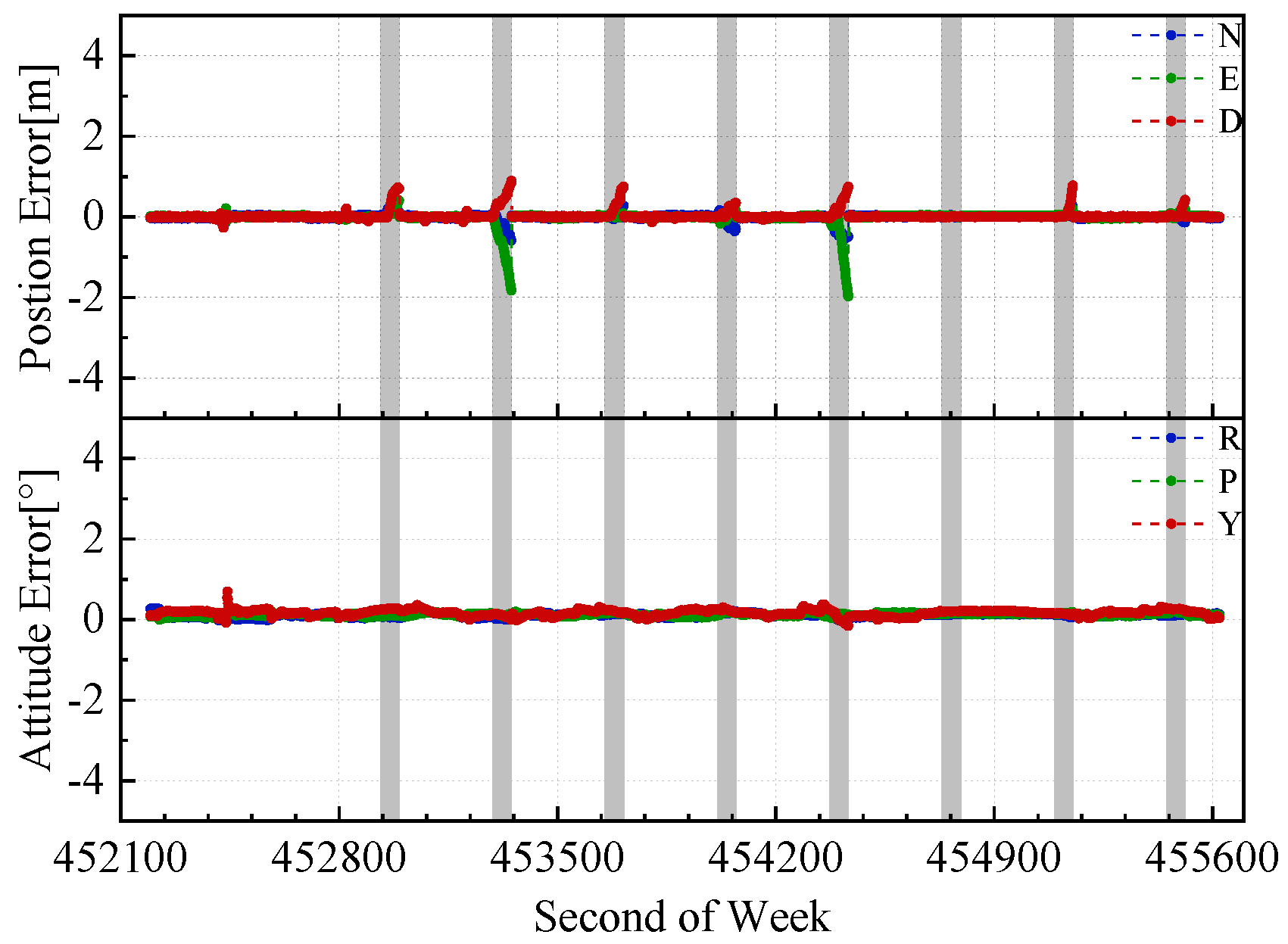
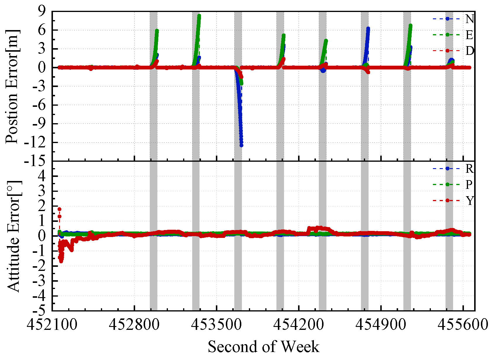
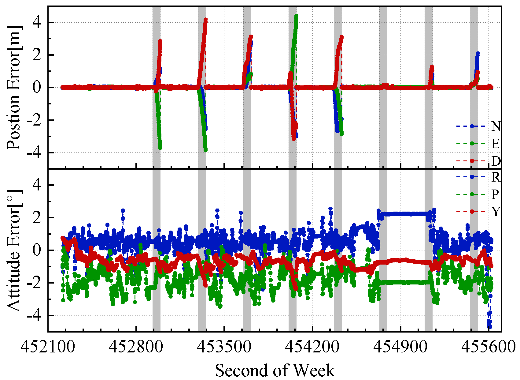
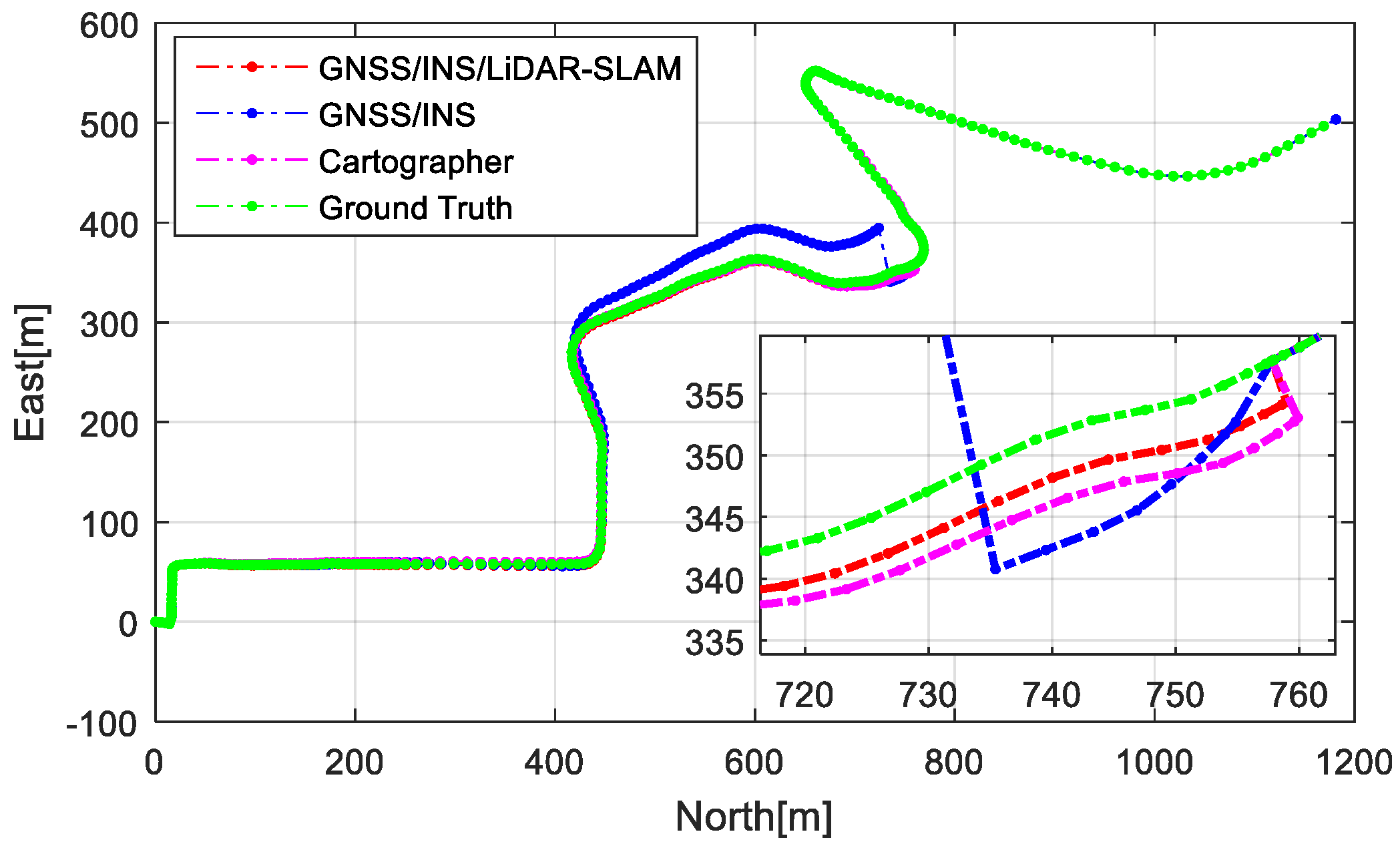
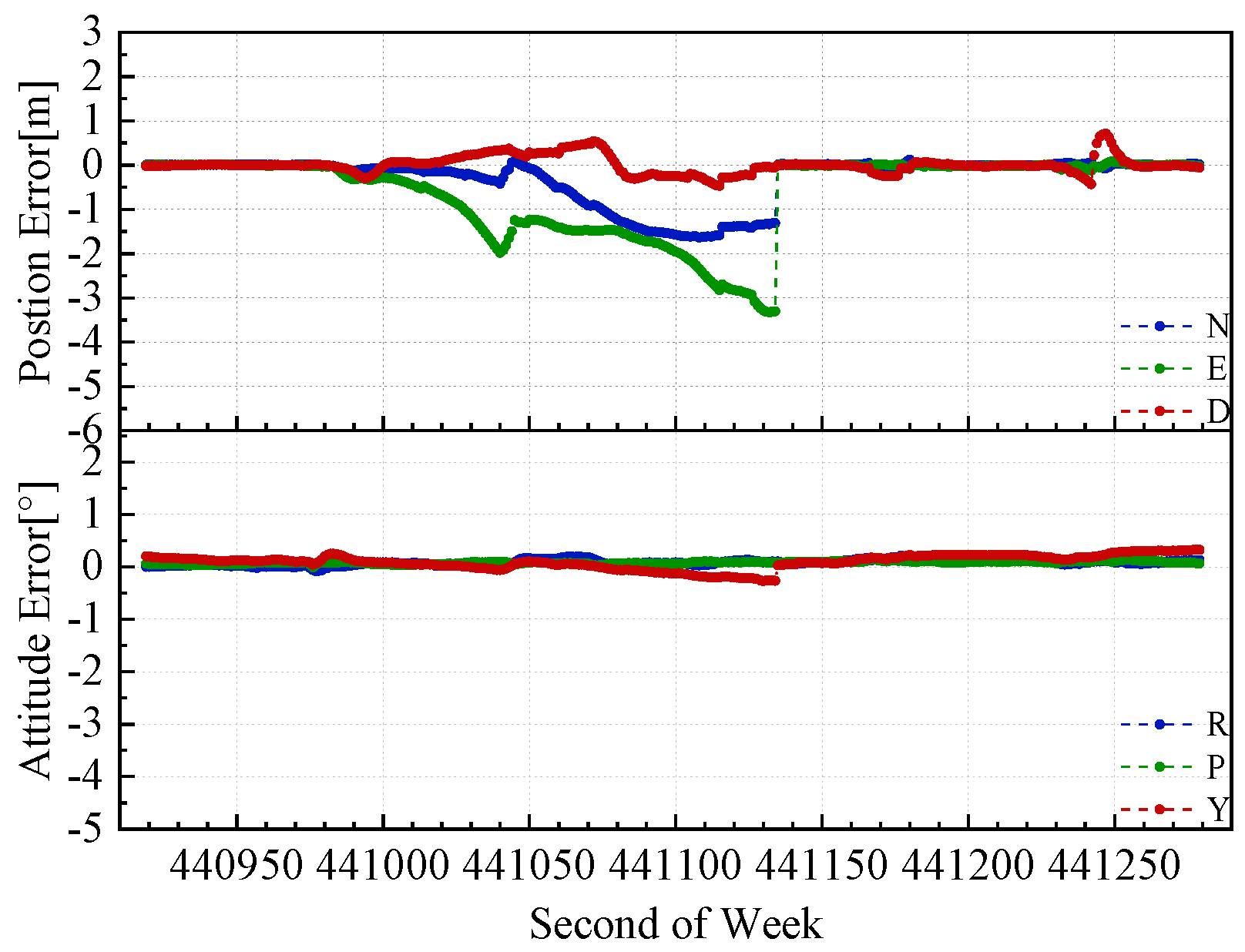
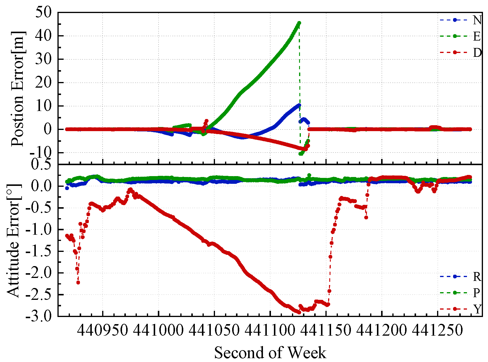
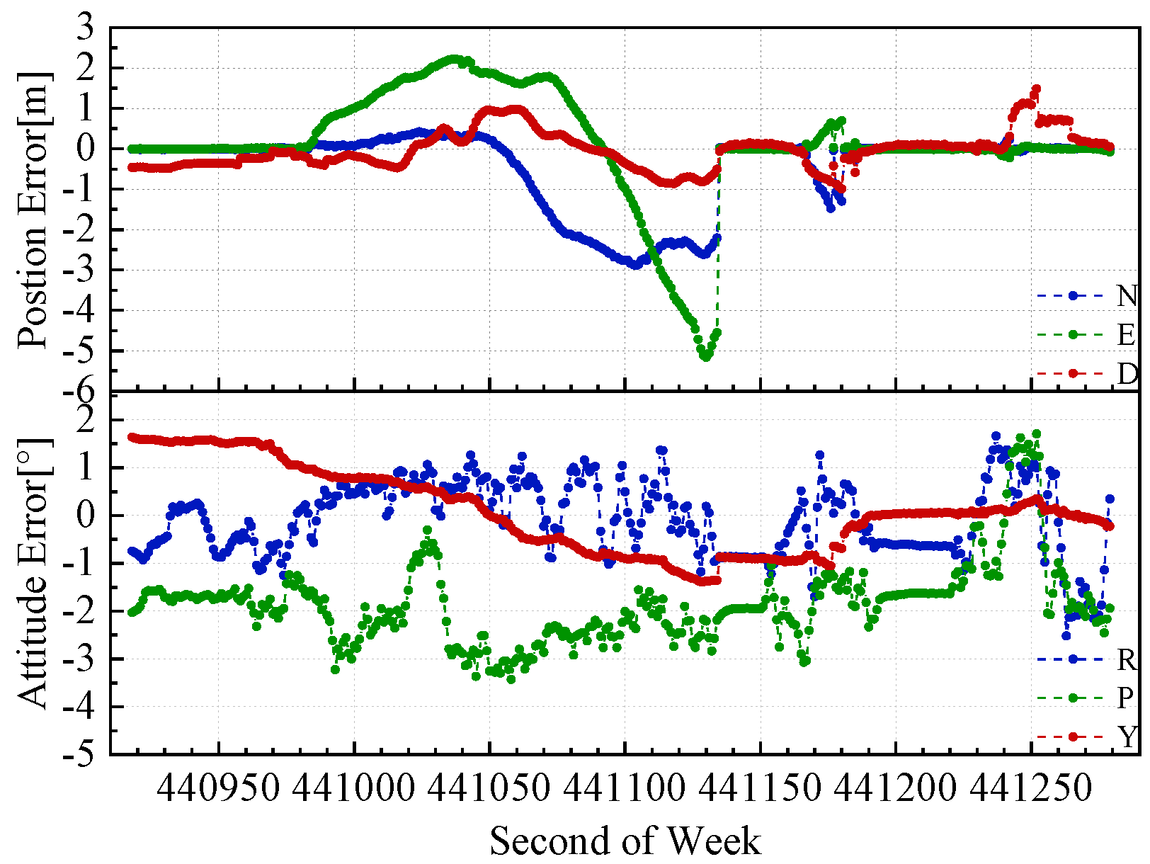
For the horizontal position error (i.e., in the North and East directions), the proposed GNSS/INS/LiDAR-SLAM integrated navigation system was the smallest, and the GNSS/INS integrated navigation system was the largest. The vertical position error of the proposed GNSS/INS/LiDAR-SLAM integrated navigation system was similar to the GNSS/INS integrated navigation system, and Cartographer had the largest vertical position error. In the sixth outage when the vehicle was at rest, the Cartographer and GNSS/INS/LiDAR-SLAM integrated navigation system significantly reduced the horizontal positioning drift with the aid of the LiDAR-SLAM compared to the GNSS/INS integrated navigation system.
(2).
Cartographer had the largest attitude error, especially in the roll and pitch, which is because Cartographer assumes low dynamic motion of the vehicle and uses gravity to solve the horizontal attitude (similar to the inclinometer principle). The attitude error of the proposed GNSS/INS/LiDAR-SLAM integrated navigation system was equivalent to that of the GNSS/INS integrated navigation system.
In the three open-sky tests, a total of 26 GNSS outages were simulated. Based on the error statistics in Table 2, the following information can be obtained by comparison with the GNSS/INS integrated navigation system:
(a)
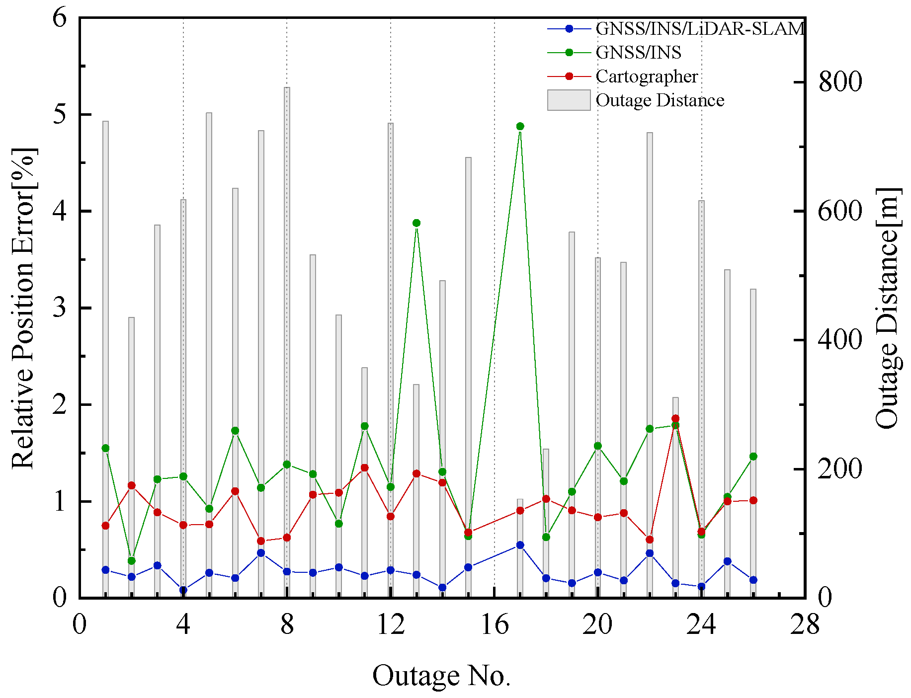
The position error RMS in the North, East and vertical directions of the proposed GNSS/INS/LiDAR-SLAM navigation system was reduced by 82.2%, 79.6%, and 17.2%, respectively. The Cartographer’s North and East position error RMS was reduced by 47.4% and 44.8%, respectively, but the vertical position error RMS is degraded by 2.3 times.
(b)
The aid of the LiDAR-SLAM did not significantly improve the attitude accuracy in the GNSS/INS/LiDAR-SLAM integrated navigation system. The RMS values of the Cartographer’s roll, pitch and yaw errors were increased by 9.5, 13.7, and 7.2 times, respectively, because of the dedicated algorithm design for low speed and smooth motion, which does not fit the test cases in this paper.
The relative position errors (i.e., percentage of position error over travel distance) in the GNSS outages are shown in Figure 12. The left y axis corresponding to the dotted lines in the figure is the relative position error of the three methods, and the right y axis corresponding to the strip is the travel distance in the GNSS outage. In the 16th outage (that is, the sixth outage in test #2, as shown in Figure 9, Figure 10 and Figure 11), the vehicle was at rest, and the relative position error was not calculated. The average relative position errors of the GNSS/INS/LiDAR-SLAM integrated navigation system, GNSS/INS integrated navigation system and Cartographer were 0.26%, 1.46%, and 0.92% of the travel distance, respectively. The aid of LiDAR-SLAM effectively reduces the relative position error in the GNSS outages.
Based on the GNSS outage simulation tests, the aid of LiDAR-SLAM can effectively reduce the position accuracy when the GNSS is unavailable. The horizontal position accuracy of the GNSS/INS/LiDAR-SLAM integrated navigation system and Cartographer was better than that of the GNSS/INS integrated navigation system. However, the Cartographer’s height and attitude error was greater than that of the GNSS/INS integrated navigation system. The reason is that Cartographer assumes that the vehicle moves at a low speed with a small acceleration; therefore, gravity is used to estimate the horizontal attitude, and the modelling for the bias of the IMU is ignored. Thus, during the tests in this paper, the horizontal attitude error and the vertical position error of Cartographer were relatively large.
In addition to the open-sky tests with simulated GNSS outage results, the trajectories of the three methods and the reference truth in the urban area test are shown in Figure 13. According to Figure 8, there were approximately 150 s of poor satellite signals in the test, and the GNSS positioning quality is generally unstable. The position and attitude errors are shown in Figure 14, Figure 15 and Figure 16, and the statistics for these errors are shown in Table 3. Similar to the three GNSS outage simulation tests, the GNSS/INS/LiDAR-SLAM integrated navigation system had the best positional accuracy. Because of the poor quality of GNSS positioning for a long time, the GNSS/INS integrated navigation system had a large yaw drift error in addition to the large position error compared to the GNSS/INS/LiDAR-SLAM integrated navigation system and Cartographer. Therefore, the aid of LiDAR-SLAM can also improve the yaw accuracy for very tough scenarios.
A solution of GNSS/LiDAR/INS navigation is demonstrated in this paper and verified by the real-world tests. There are not too much complicated theoretical conclusions, such as the observability, which should be validated by controllable simulation data have been proposed in this paper. And because in the simple and controllable simulated environment, error models and parameters are clear, the algorithms always get a good result than in real scenarios and it’s not persuasive. Consequently, to indicate the performance of this solution, the data collected in real-world scenarios is convincing and this is the only data source in this paper. In addition, the system in this paper requires the raw LiDRA data, which is not easy to simulate.
The results of the four vehicle tests (three open-sky and one urban street) have shown that the position and attitude accuracy of the proposed GNSS/INS/LiDAR-SLAM integrated navigation system is the best, especially in a weak or blocked GNSS signal environment. Cartographer has the largest roll, pitch and elevation errors because the motion model of the algorithm is only suitable for low-speed motion. Due to the lack of aiding information, the GNSS/INS integrated navigation system gradually degrades the position and attitude when GNSS is not available, and LiDAR-SLAM assistance can play a significant role in maintaining navigation accuracy.

5. Conclusions

In this paper, a GNSS/INS/LiDAR-SLAM integrated navigation system is proposed. The MEMS-IMU mechanization is applied for pose estimation. Through graph optimization, the GNSS position, IMU preintegration results and the relative pose obtained from LiDAR scan matching are fused. In addition, the use of a sliding window ensures that the computational load of the graph optimization does not increase with time. The vehicle tests show that the GNSS/INS/LiDAR-SLAM integrated navigation system can effectively reduce the position errors in the horizontal directions during the GNSS outage periods compared with the GNSS/INS integrated navigation system. For the position error in the vertical direction and the attitude error, the two systems perform similarly. In addition, compared with the benchmark method of GNSS/INS/LiDAR-Google Cartographer, the use of the IMU information in the proposed algorithm is more reasonable and sufficient, thus improving both the position and attitude accuracies. Finally, the relative position error of the proposed GNSS/INS/LiDAR-SLAM method during the GNSS outage was reduced from 1.46% (GNSS/INS) to 0.92% (Cartographer) to 0.26% of the travel distance.
For future works, the GNSS/INS/LiDAR integrated navigation system in this paper cannot yet eliminate the dynamic objects from the environment. Therefore, it is necessary to add the recognition and elimination mechanism of dynamic objects in the environment. Furthermore, a procreated background map may be added to improve the robustness and navigation positioning accuracy of the integrated navigation system, such as for applications for autodrive and mobile robots.

Author Contributions

L.C. and X.N. conceived and designed the experiments, wrote the paper, and performed the experiments; T.L. performed the land vehicle tests and provided the LiDAR, IMU, and GNSS raw data; and J.T. and C.Q. reviewed the paper and gave constructive advice.

Funding

This research was funded by the “National Key Research and Development Program” (No. 2016YFB0501803 and No. 2016YFB0502202) and the “Fundamental Research Funds for the Central Universities” (No. 2042018KF0242).

Conflicts of Interest

The authors declare no conflict of interest.

References

  1. Shin, E.-H. Estimation Techniques for Low-Cost Inertial Navigation; The University of Calgary: Calgary, Canada, 2005. [Google Scholar]
  2. Pagliaria, D.; Pinto, L.; Reguzzoni, M.; Rossi, L. Integration of kinect and low-cost gnss for outdoor navigation. Int. Arch. Photogramm. Remote Sens. Spat. Inf. Sci. 2016, XLI-B5, 565–572. [Google Scholar] [CrossRef]
  3. Rossi, L.; De Gaetani, C.; Pagliari, D.; Realini, E.; Reguzzoni, M.; Pinto, L. Comparison between rgb and rgb-d cameras for supporting low-cost gnss urban navigation. Int. Arch. Photogramm. Remote Sens. Spat. Inf. Sci. 2018, 42, 991–998. [Google Scholar] [CrossRef]
  4. Cadena, C.; Carlone, L.; Carrillo, H.; Latif, Y.; Scaramuzza, D.; Neira, J.; Reid, I.; Leonard, J.J. Past, Present, and Future of Simultaneous Localization and Mapping: Toward the Robust-Perception Age. IEEE Trans. Robot. 2016, 32, 1309–1332. [Google Scholar] [CrossRef] [Green Version]
  5. Walter, M.R.; Eustice, R.M.; Leonard, J.J. Exactly Sparse Extended Information Filters for Feature-based SLAM. Int. J. Robot. Res. 2007, 26, 335–359. [Google Scholar] [CrossRef]
  6. Deschaud, J.-E. IMLS-SLAM: Scan-to-model matching based on 3D data. In Proceedings of the 2018 IEEE International Conference on Robotics and Automation (ICRA2018), Brisbane, QL, Australia, 21–25 May 2018; pp. 2480–2485. [Google Scholar]
  7. Behley, J.; Stachniss, C. Efficient Surfel-based Slam Using 3d Laser Range Data in Urban Environments. Available online: http://roboticsproceedings.org/rss14/p16.pdf (accessed on 25 April 2019).
  8. Zhang, J.; Singh, S. LOAM: Lidar Odometry and Mapping in Real-time. In Proceedings of the Robotics: Science and Systems, Berkeley, CA, USA, 14–16 July 2014; 2014. [Google Scholar] [Green Version]
  9. Qin, T.; Li, P.; Shen, S. VINS-Mono: A Robust and Versatile Monocular Visual-Inertial State Estimator. IEEE Trans. Robot. 2018, 34, 1004–1020. [Google Scholar] [CrossRef]
  10. Zhang, J.; Singh, S. Visual-lidar odometry and mapping: Low-drift, robust, and fast. In Proceedings of the 2015 IEEE International Conference on Robotics and Automation (ICRA2015), Seattle, WA, USA, 26–30 May 2015; pp. 2174–2181. [Google Scholar]
  11. Martínez, J.L.; González, J.; Morales, J.; Mandow, A.; García-Cerezo, A.J. Mobile robot motion estimation by 2D scan matching with genetic and iterative closest point algorithms. J. Field Robot. 2006, 23, 21–34. [Google Scholar] [CrossRef]
  12. Censi, A. An ICP variant using a point-to-line metric. In Proceedings of the 2008 IEEE International Conference on Robotics and Automation, Pasadena, CA, USA, 19–23 May 2008. [Google Scholar]
  13. Aleksandr, S.; Haehnel, D.; Thrun, S. Generalized-ICP. In Proceedings of the Robotics: Science and Systems, Seattle, WA, USA, 28 June–1 July 2009; p. 435. [Google Scholar]
  14. Burguera, A.; González, Y.; Oliver, G. On the use of likelihood fields to perform sonar scan matching localization. Auton. Robot. 2009, 26, 203–222. [Google Scholar] [CrossRef]
  15. Hess, W.; Kohler, D.; Rapp, H.; Andor, D. Real-time loop closure in 2D LIDAR SLAM. In Proceedings of the IEEE International Conference on Robotics and Automation, Stockholm, Sweden, 16–21 May 2016; pp. 1271–1278. [Google Scholar]
  16. Gao, Y.; Liu, S.; Atia, M.M.; Noureldin, A. INS/GPS/LiDAR Integrated Navigation System for Urban and Indoor Environments Using Hybrid Scan Matching Algorithm. Sensors 2015, 15, 23286–23302. [Google Scholar] [CrossRef] [PubMed] [Green Version]
  17. Durrant-Whyte, H.; Bailey, T. Simultaneous localization and mapping: Part I. IEEE Robot. Autom. Mag. 2006, 13, 99–110. [Google Scholar] [CrossRef]
  18. Qian, C.; Liu, H.; Tang, J.; Chen, Y.; Kaartinen, H.; Kukko, A.; Zhu, L.; Liang, X.; Chen, L.; Hyyppä, J. An integrated GNSS/INS/LiDAR-SLAM positioning method for highly accurate forest stem mapping. Remote Sens. 2016, 9, 3. [Google Scholar] [CrossRef]
  19. Shamsudin, A.U.; Ohno, K.; Hamada, R.; Kojima, S.; Westfechtel, T.; Suzuki, T.; Okada, Y.; Tadokoro, S.; Fujita, J.; Amano, H. Consistent map building in petrochemical complexes for firefighter robots using SLAM based on GPS and LIDAR. Robomech. J. 2018, 5, 7. [Google Scholar] [CrossRef] [Green Version]
  20. Kukko, A.; Kaijaluoto, R.; Kaartinen, H.; Lehtola, V.V.; Jaakkola, A.; Hyyppä, J. Graph SLAM correction for single scanner MLS forest data under boreal forest canopy. Isprs J. Photogramm. Remote Sens. 2017, 132, 199–209. [Google Scholar] [CrossRef]
  21. Pierzchała, M.; Giguère, P.; Astrup, R. Mapping forests using an unmanned ground vehicle with 3D LiDAR and graph-SLAM. Comput. Electron. Agric. 2018, 145, 217–225. [Google Scholar] [CrossRef]
  22. Cartographer. Latest. Available online: https://google-cartographer.readthedocs.io/en/latest/ (accessed on 9 July 2018).
  23. Forster, C.; Carlone, L.; Dellaert, F.; Scaramuzza, D. On-Manifold Preintegration for Real-Time Visual--Inertial Odometry. IEEE Trans. Robot. 2015, 33, 1–21. [Google Scholar] [CrossRef]
  24. Yahao, C. Algorithm Implementation of Pseudorange Differential BDS/INS Tightly-Coupled Integration and GNSS Data Quality Control Analysis; Wuhan University: Wuhan, China, 2013. [Google Scholar]
  25. Jun, W.; Gongmin, Y. Strapdown Inertial Navigation Algorithm and Integrated Navigation Principles; Northwestern Polytechnical University Press Co. Ltd.: Xi’an, China, 2016. [Google Scholar]
  26. Dehai, Z. Point Cloud Library PCL Learning Tutorial; Beihang University Press: Beijing, China, 2012. [Google Scholar]
  27. Slerp. Available online: https://en.wikipedia.org/wiki/Slerp (accessed on 2 October 2018).
  28. Olson, E.B. Real-time correlative scan matching. In Proceedings of the IEEE International Conference on Robotics and Automation, Kobe, Japan, 12–17 May 2009; pp. 1233–1239. [Google Scholar]
  29. Ceres Solver, 1.14. Available online: http://ceres-solver.org (accessed on 23 March 2018).
  30. Lekien, F.; Marsden, J.E. Tricubic Interpolation in Three Dimensions. Int. J. Numer. Methods Eng. 2010, 63, 455–471. [Google Scholar] [CrossRef]
  31. Clausen, J. Branch and Bound Algorithms—Principles and Examples. Parallel Process. Lett. 1999, 22, 658–663. [Google Scholar]
  32. Xiangyuan, K.; Jiming, G.; Zongquan, L. Foundation of Geodesy, 2nd ed.; Wuhan University Press: Wuhan, China, 2010. [Google Scholar]
  33. Sola, J. Quaternion kinematics for the error-state Kalman filter. arXiv 2017, arXiv:1711.02508. [Google Scholar]
  34. Yongyuan, Q. Kalman Filter and Integrated Navigation Principle; Northwestern Polytechnical University Press Co. Ltd.: Xi’an, China, 2000. [Google Scholar]
  35. Sibley, G.; Matthies, L.; Sukhatme, G. Sliding window filter with application to planetary landing. J. Field Robot. 2010, 27, 587–608. [Google Scholar] [CrossRef]
  36. Zhang, F. The Schur Complement and Its Applications; Springer: New York, NY, USA, 2005. [Google Scholar]
  37. Eckenhoff, K.; Paull, L.; Huang, G. Decoupled, consistent node removal and edge sparsification for graph-based SLAM. In Proceedings of the IEEE/RSJ International Conference on Intelligent Robots and Systems, Daejeon, Korea, 9–14 October 2016; pp. 3275–3282. [Google Scholar]
Figure 1. System overview of Global Navigation Satellite System (GNSS)/Inertial Navigation System (INS)/Light Detection and Ranging (LiDAR)-Simultaneous Localization and Mapping (SLAM) integrated navigation.
Remotesensing 11 01009 g001
Figure 2. Flow chart of local registration.
Remotesensing 11 01009 g002
Figure 3. Schematic diagram of the probability map.
Remotesensing 11 01009 g003
Figure 4. Schematic diagram of submaps and nodes.
Remotesensing 11 01009 g004
Figure 5. Experimental platform.
Remotesensing 11 01009 g005
Figure 6. Test trajectory in the open-sky environment.
Remotesensing 11 01009 g006
Figure 7. Test trajectory in the urban area.
Remotesensing 11 01009 g007
Figure 8. Number of satellites in the urban area.
Remotesensing 11 01009 g008
Figure 9. Position and attitude errors of the GNSS/INS/LiDAR-SLAM integrated navigation system in the GNSS outage simulation test #2.
Remotesensing 11 01009 g009
Figure 10. Position and attitude errors of the GNSS/INS integrated navigation system in the GNSS outage simulation test #2.
Remotesensing 11 01009 g010
Figure 11. Position and attitude errors of Cartographer in the GNSS outage simulation test #2.
Remotesensing 11 01009 g011
Figure 12. Relative position errors in the GNSS outage simulation tests.
Remotesensing 11 01009 g012
Figure 13. Trajectories in the urban area test.
Remotesensing 11 01009 g013
Figure 14. Position and attitude errors of the GNSS/INS/LiDAR-SLAM integrated navigation system in the urban area test.
Remotesensing 11 01009 g014
Figure 15. Position and attitude errors of the GNSS/INS integrated navigation system in the urban area test.
Remotesensing 11 01009 g015
Figure 16. Position and attitude errors of Cartographer in the urban area test.
Remotesensing 11 01009 g016
Table 1. Technical Parameters of LD-A15 and NV-POS1100.
IMUBiasRandom Walk
Gyro. [°/h]Acc. [mGal] Angular   [ ° / h ] Velocity   [ m / s / h ]
LD-A15
(Reference system)
0.02150.0030.03
NV-POS1100
(Tested system)
1010000.20.18
Table 2. Errors statistics for the GNSS outage simulation tests.
Position Error [m]Attitude Error [°]
NEDRPY
Proposed GNSS/INS/LiDAR-SLAMRMS0.9431.1140.7210.1510.1820.213
MAX3.2123.1611.1120.2340.2530.323
GNSS/INSRMS5.2985.4690.8710.1360.1750.225
MAX12.47511.3282.1850.1970.2170.562
CartographerRMS2.7893.0192.8981.4382.5891.865
MAX4.8354.4394.1692.3203.6022.896
Table 3. Error statistics for the urban area test.
Position Error [m]Attitude Error [°]
NEDRPY
Proposed GNSS/INS/LiDAR-SLAMRMS0.6151.1050.1980.0990.0830.166
MAX1.6353.3280.7070.2150.1420.323
GNSS/INSRMS2.03111.7572.3890.1160.1601.375
MAX10.33845.4858.4990.2230.2532.910
CartographerRMS1.0511.3950.4630.7802.0420.867
MAX2.8915.1661.4882.5173.4271.637

